Non-Bayesian Activity Detection, Large-Scale Fading Coefficient Estimation, and Unsourced Random Access with a Massive MIMO Receiver

Abstract

In this paper, we study the problem of user activity detection and large-scale fading coefficient estimation in a random access wireless uplink with a massive MIMO base station with a large number $M$ of antennas and a large number of wireless single-antenna devices (users). We consider a block fading channel model where the $M$-dimensional channel vector of each user remains constant over a coherence block containing $L$ signal dimensions in time-frequency. In the considered setting, the number of potential users $K_{\text{tot}}$ is much larger than $L$ but at each time slot only $K_{a}\ll K_{\text{tot}}$ of them are active. Previous results, based on compressed sensing, require that $K_{a}\leq L$, which is a bottleneck in massive deployment scenarios. In this work, we show that such limitation can be overcome when the number of base station antennas $M$ is sufficiently large. More specifically, we prove that with a coherence block of dimension $L$ and a number of antennas $M$ such that $K_{a}/M=o(1)$, one can identify $K_{a}=O(L^{2}/\log^{2}(\frac{K_{\text{tot}}}{K_{a}}))$ active users, which is much larger than the previously known bounds. We also provide two algorithms. One is based on Non-Negative Least-Squares, for which the above scaling result can be rigorously proved. The other consists of a low-complexity iterative componentwise minimization of the likelihood function of the underlying problem. While for this algorithm a rigorous proof cannot be given, we analyze a constrained version of the Maximum Likelihood (ML) problem (a combinatorial optimization with exponential complexity) and find the same fundamental scaling law for the number of identifiable users. Therefore, we conjecture that the low-complexity (approximated) ML algorithm also achieves the same scaling law and we demonstrate its performance by simulation. We also compare the discussed methods with the (Bayesian) MMV-AMP algorithm, recently proposed for the same setting, and show superior performance and better numerical stability. Finally, we use the discussed approximated ML algorithm as the inner decoder in a concatenated coding scheme for unsourced random access, a grant-free uncoordinated multiple access scheme where all users make use of the same codebook, and the receiver must produce the list of transmitted messages, irrespectively of the identity of the transmitters. We show that reliable communication is possible at any $E_{b}/N_{0}$ provided that a sufficiently large number of base station antennas is used, and that a sum spectral efficiency in the order of $\mathcal{O}(L\log(L))$ is achievable.

I Introduction

One of the paradigms of modern machine-type communications [3] consists of a very large number of devices (here referred to as “users”) with sporadic data. Typical examples thereof are Internet-of-Things (IoT) applications, wireless sensors deployed to monitor smart infrastructure, and wearable biomedical devices [4]. In such scenarios, a Base Station (BS) should be able to collect data from a large number of devices. However, due to the sporadic nature of the data generation and communication, allocating some dedicated transmission resource to all users in the system may be extremely wasteful. In most wireless systems, a dedicated random access slot (or logical channel) is used to allow the users with some data to transmit to ask the Base Station (BS) to be granted access to some transmission resource, which is successively released. For example, most systems operating today, such as (3G, 4G-LTE, and 5G New Radio, follow this paradigm [5, 6]. As an alternative, the random access channel itself can be used to directly transmit data in a grant-free mode. As yet another twist in the system classification of random access schemes, a recently proposed information theoretic model referred to as unsourced random access assumes grant-free operations and, in addition, that all users make use of exactly the same codebook [7]. Unsourced random access is motivated by an IoT scenario where millions of cheap devices have their codebook hardwired at the moment of production, and are then disseminated into the environment. In this case, the BS receiver must determine the list of transmitted messages irrespectively of the identity of the active users.

In this paper, we are mainly interested in the problem of Activity Detection (AD) from a dedicated pilot slot. The AD function can be included either in a more traditional granted resource random access protocol, or in a grant-free protocol. In the second part of the paper, we shall use the proposed AD scheme as the inner code/decoder of a concatenated coding scheme specifically addressing the problem of unsourced random access.

AD is a fundamental challenge in massive sensor deployments and random access scenarios to be expected for IoT (see, e.g., [8, 9, 10, 11, 12, 13] for some recent works) We consider a classical block-fading wireless communication channel between the users and the BS [14], where the channel coefficients remain constant over coherence blocks consisting of $L$ signal dimensions in the time-frequency domain, and change randomly from block to block according to a stationary ergodic process [14]. A fundamental limitation when considering a single-antenna BS is that the required signal dimension $L$ to identify reliably a subset of $K_{a}$ active users among a set consisting of $K_{\text{tot}}$ potentially active users scales as $L=O(K_{a}\log(\frac{K_{\text{tot}}}{K_{a}}))$, thus, almost linearly with $K_{a}$. To keep up with the scaling requirements in practical applications where $K_{a}$ may be of the order of $10^{2}$ and $K_{\text{tot}}$ may be of the order of $10^{4}$ – $10^{5}$, it is crucial to overcome this limitation in an efficient way that does not require devoting too many pilot dimension to AD.

In a series of recent works [12, 13, 15], AD with a massive MIMO BS with a large number $M$ of antennas was considered and formulated as a Multiple Measurement Vector (MMV) [16, 17, 18] problem. In these works, the activity detection problem is formulated in a Bayesian way and a method based on an MMV suited version of Approximated Message Passing (MMV-AMP) followed by a componentwise Neyman-Pearson activity estimation by suitable thresholding is proposed. There are several issues with this problem formulation and with the proposed MMV-AMP algorithm. First, the algorithm needs to treat the Large-Scale Fading Coefficients (LSFCs) as either as deterministic known quantities, or as random quantities whose prior distribution is known. In practice, it is not easy to individually measure the LSFC from all $K_{\rm tot}$ users, especially when they stay silent for a long time and move or the propagation conditions change. Also, the typical distance dependent pathloss and log-normal shadowing laws used in standard models are not quite representative of specific environments and the prior ensemble distribution would assume some spatial distribution (e.g., uniform in a cell as in [12, 15]) which is not always the case. Furthermore, the MMV-AMP algorithm can be analyzed via the state evolution method [12, 15] in the large-dimensional regime where $L,K_{a}$, and $K_{\rm tot}$ grow to infinity at fixed ratios $\frac{K_{a}}{L}\to\alpha$ and $\frac{K_{\text{tot}}}{L}\to\beta$ with $\alpha,\beta\in(0,\infty)$ while $M$ is finite. Therefore, the regime of $L$ linear in $K_{a}$ (which we wish to beat) is somehow unavoidable in this type of analysis. Finally, it turns out that in practical scenarios where $M$ is fairly larger than $L$ and comparable to $K_{a}$ (which are scenarios of interest in our work and in practical scenarios, where $L$ is between 50 and 200 and $M$ can be up to 256 antennas [19, 20, 21]), MMV-AMP is quite numerically unstable and gives pathological and unpredictable behaviors that one would like definitely to avoid in a real-world implementation.

In this work, we consider a non-Bayesian approach, treating the LSFCs as deterministic unknown. We use tools from Compressed Sensing (CS) to provide a stability analysis of the LSFC estimation and AD problem for finite SNR and finite number of antennas $M$. As a consequence of this analysis, we are able to show that with a coherence block of dimension $L$, and with a sufficient number of BS antennas $M$ with $K_{a}/M=o(1)$, one can estimate the LSFC, and thus identify the activity, of up to $K_{a}=O(L^{2}/\log^{2}(\frac{K_{\text{tot}}}{K_{a}}))$ active users among $K_{\text{tot}}$ users. These results are obtained by analyzing a Non-Negative Least-Squares (NNLS) algorithm applied to the sample covariance information, which was recently considered for LSFC estimation in [22]. The analysis in [22] showed, that with a random choice of pilot sequences the LSFCs of up to $K_{a}=\mathcal{O}(L^{2})$ users could be estimated, but the proof was limited by the assumptions of $K_{a}=K_{\text{tot}}$,$K_{\text{tot}}\leq L^{2}$ and $M\to\infty$. Our result lifts all these restrictions and shows that $K_{\text{tot}}$ may be potentially much larger than $L^{2}$ and $K_{a}$, where one needs to pay only a logarithmic penalty $O(\log^{2}(\frac{K_{\text{tot}}}{K_{a}}))$ for increasing the total number of users $K_{\text{tot}}$. This makes the proposed scheme very attractive for IoT setups, in which the number of active users $K_{a}$ as well as the total number of users $K_{\text{tot}}$ may be extremely large.

Furthermore, we propose to use an improved algorithm for AD based on the Maximum-Likelihood (ML) estimation of the LSFCs of the active users. The resulting likelihood maximization is a non-convex problem, that can be solved (approximately) by iterative componentwise minimization. This yields an iterative scheme based on rank-1 updates whose complexity is comparable to that of NNLS and MMV-AMP. Extensive numerical simulations show that the ML algorithm is superior to NNLS and to MMV-AMP in any regime, and does not suffer from the ill-conditioned behavior of MMV-AMP for the case of large $M$. The componentwise optimization of the log-likelihood function was developed in [23, 24, 25, 26], where the sparse Bayesian learning (SBL) framework was introduced to find the optimal vector of weights in a linear regression problem. In the SBL framework it is assumed that the weight vector follows a Gaussian prior distribution with zero mean and a diagonal covariance matrix. The entries of the covariance matrix are estimated by maximizing the likelihood of the data. It was observed that the likelihood function maximization yields a very sparse result, which is a desirable property in statistical learning. The maximum of the likelihood function can be computed iteratively by following the general expectation-maximization (EM) framework [27, 28], but it was found that a componentwise optimization leads to faster convergence while still being guaranteed to converge to at least a local maximum of the likelihood function [24], similar to EM. The SBL framework was extended and applied to basis selection [29], compressed sensing [30] and also the MMV problem [31], where the latter was termed M-SBL. Here, the task is to recover ${\bf X}\in\mathbb{C}^{K_{\text{tot}}\times M}$ (here we stick to the notation introduced in this paper) from multiple measurements ${\bf Y}\in\mathbb{C}^{L\times M}$ of the form

$${\bf Y}={\bf A}{\bf X}+{\bf Z}$$ (1)

Following the SBL framework, it is assumed that the rows of ${\bf X}$ are distributed according to

$${\bf X}_{:,i}\sim\mathcal{CN}(0,\gamma_{i}{\bf I}_{M}).$$ (2)

Note, that in the literature the term M-SBL has often been used ambiguously to refer to the ML estimate of the parameters $\gamma_{i}$ as well as to the algorithm used to find this solution, which may be either coordinate-wise optimization or EM. Both of these algorithms lead to similar solutions [31], but here we adopt the componentwise optimization algorithm, since it can be efficiently implemented using rank-1 updates leading to a significant complexity reduction compared to the EM version.

Let ${\bf X}$ have $K_{a}$ non-zero rows. The identifiability limits of the ML solution of M-SBL were analysed in [32, 33, 34, 35, 36]. While the early work [32] was restricted to the case $K_{a}\leq L$, [33] made the distinction between recovering ${\bf X}$, which necessarily requires $K_{a}\leq L$, and recovering the vector ${\boldsymbol{\gamma}}=(\gamma_{1},...,\gamma_{K_{\text{tot}}})$. It was noticed in [33] that the recovery of ${\boldsymbol{\gamma}}$ is governed by the properties of the Khatri-Rao product ${\bf A}\odot{\bf A}$ and it was proven that, with a random choice of ${\bf A}$, up to $K_{a}=\mathcal{O}(L^{2})$ non-zero entries of ${\boldsymbol{\gamma}}$ can be recovered uniquely if the covariance matrix of ${\bf Y}$ is known exactly. The proof of [33] (similar proofs were given independently in [22, 36]) is based on the fact that any $2K_{a}$ columns of ${\bf A}\odot{\bf A}$ are linearly independent almost surely for $K_{a}$ up to $\mathcal{O}(L^{2})$. This proof deals only with the identifiability, i.e., it does not apply to a specific recovery algorithm and does not take into account the uncertainty in estimating the covariance matrix of ${\bf Y}$, and therefore gives no clue on the robustness (error bound) of the recovery. It is well known in the compressed sensing literature that stronger conditions are needed to guarantee algorithmic robust recovery [37]. Upper and lower bounds on the performance of the ML solution of M-SBL for the noisy case have been derived in [32] for $K_{a}\leq L$ and in [35] for $K_{a}=\mathcal{O}(L^{2})$, but these bounds contained parameters which were exponentially hard to compute for a given matrix ${\bf A}$ and so no concrete scaling of $K_{a}$ could be given. A coherence based argument was given in [33] to analyse the performance of a covariance based LASSO algorithm, but it was only possible to guarantee recovery for up to $K_{a}=\mathcal{O}(L)$ coefficients. This is a well known limitation of coherence based arguments, known as the ”square-root bottleneck” [37]. In this work we are able to circumvent this bottleneck by proving the restricted isometry property (RIP) of a properly centered and rescaled version of ${\bf A}\odot{\bf A}$ for random ${\bf A}$. This allows us to prove recovery guarantees for both the NNLS algorithm of [22] and a constrained variant of the ML solution, showing that $K_{a}=\mathcal{O}(L^{2})$ coefficients can be recovered. Although the constrained ML yields a combinatorial minimization with exponential complexity and therefore is not useful in practice, we can show that the scaling law for successful detection of the activity pattern of the constrained ML scheme is the same (up to logarithmic factors in the scaling of $M$) as what was found for NNLS. Therefore, we conjecture that the (low-complexity) ML algorithm achieves the same scaling law. We provide an intuitive argument which, at least heuristically, explains why we expect the componentwise optimization to converge to the global optimum in the considered scaling regime. We would like to mention that an analysis of the constrained ML estimator was recently presented in [38]. However, the results in [38] are based on a RIP result that was first claimed and then withdrawn by the same authors [39]. Hence, our result based on a new RIP and a few consequent modifications which we duly prove, essentially rigorizes the analysis presented in [38].

The full characterisation of the global (unconstrained) ML solution and the conditions under which the iterative estimate coincides with it remains open. Some progress has recently been made in [40], where it was shown the global optimality of the algorithmic solution can be checked, given ${\bf A}$ and the true ${\boldsymbol{\gamma}}^{\circ}$, by a linear feasibility program. In contrast, our recovery guarantees for the NNLS algorithm hold for all $K_{a}$-sparse ${\boldsymbol{\gamma}}$ and are given in closed form (up to unspecified constants). Based on the asymptotic Gaussianity of ML estimators in general, it was shown in [40] that for large $M$ the distribution of the ML estimation error, for a fixed ${\boldsymbol{\gamma}}^{\circ}$, can be characterized numerically by the solution of a quadratic program.

The coordinate-wise optimization algorithm for M-SBL was also independently re-discovered and investigated in the context of source localisation [41, 42, 43]. It was noted in [41] that the update equation can be equivalently derived by an iterative weighted least-squares (WLS) approach, which asymptotically minimizes the variance of the estimation. The resulting algorithm has therefore been called iterative asymptotic sparse minimum variance stochastic ML (SAMV-SML). Recently, in [44] a similar WLS estimator was derived and an iterative algorithm was given to find an approximation of the WLS minimizer. The performance reported was very similar to M-SBL, but at a much higher complexity-per-iteration of $\mathcal{O}(L^{4}K_{\text{tot}}^{2})$, compared to $\mathcal{O}(L^{2}K_{\text{tot}})$ for the coordinate-wise optimization with rank-1 updates.

Finally, we focus on unsourced random access with a massive MIMO BS. It is evident that the AD problem and the random access problem are related. In fact, one can immediately obtain a random access scheme from an AD scheme as follows: assign to each user a unique set of pilot signature sequences (codewords), such that a user, when active, will transmit the signature corresponding to its information message. Since the number of pilot signatures is $K_{\rm tot}\gg K_{a}$, this scheme involves only an expansion of the number of total users from $K_{\rm tot}$ to $K^{\prime}_{\rm tot}=K_{\rm tot}2^{B}$ where $B$ is the number of per-message information bits. This idea was recently presented in [10], where the MMV-AMP detector of [18, 12, 15] was used at the receiver side. While conceptually simple, this approach has two major drawbacks: 1) even for relatively small information packets (e.g., $B=100$ bits), the dimension of the pilot matrix is too large for practical computational algorithms; 2) each user has a different set of pilot sequences, and therefore the scheme is not compliant with the basic assumption of unsourced random access, that users have all the same codebook.

In contrast, we present a novel scheme, build upon the concatenated coding approach of [45], that does not incur in the large dimension problem and is independent of the number of “inactive” users. In our scheme, the message of $B$ bits of each user is split into a sequence of submessages of potentially different lengths. These submessages are encoded via a tree code (the same for each user), such that the encoded blocks have the same length of $J$ bits. Then, each user transmits its sequence of $J$-bits blocks in consecutive blocks of $L$ dimensions, using the same $L\times 2^{J}$ pilot matrix (where blocks are encoded in the matrix columns). The inner detector perform our ML activity detection scheme and for each slot recovers the set of active columns of the pilot matrix. These are passed to the outer tree code, which recovers each user message by “stitching together” the sequence of submessages. We show that an arbitrary small probability of error is achievable at any $E_{b}/N_{0}$ provided that a sufficiently large number of base station antennas is used, and that the sum spectral efficiency can grow as $\mathcal{O}(L\log(L))$. This can be achieved in a completely non-coherent way, i.e. it is at no point necessary to estimate the channel matrix (small-scale fading coefficients). These are important properties to enable easily deployable, low-latency, energy efficient communication in an IoT setting.

I-A Notation

We represent scalar constants by non-boldface letters (e.g., $x$ or $X$), sets by calligraphic letters (e.g., ${\cal X}$), vectors by boldface small letters (e.g., ${\bf x}$), and matrices by boldface capital letters (e.g., ${\bf X}$). We denote the $i$-th row and the $j$-th column of a matrix ${\bf X}$ with the row-vector ${\bf X}_{i,:}$ and the column-vector ${\bf X}_{:,j}$ respectively. We denote a diagonal matrix with elements $(s_{1},s_{2},\dots,s_{k})$ by ${\text{diag}}(s_{1},\dots,s_{k})$. We denote the vectorization operator by ${\rm vec}(.)$. We denote the $\ell_{p}$-norm of a vector ${\bf x}$ and the Frobenius norm of a matrix ${\bf X}$ by $\|{\bf x}\|_{{p}}$ and $\|{\bf X}\|_{{p}}$ resp. $\|{\bf x}\|_{0}:=|\{i:x_{i}\neq 0\}|$ denotes the number of non-zero entries of a vector ${\bf x}$. The operator norm of a matrix ${\bf X}$ is denoted by $\|{\bf X}\|_{op}$. The $k\times k$ identity matrix is represented by ${\bf I}_{k}$. For an integer $k>0$, we use the shorthand notation $[k]$ for $\{1,2,\dots,k\}$. We use superscripts $(\cdot)^{\sf T}$ and $(\cdot)^{{\sf H}}$ for transpose and Hermitian transpose. $\odot$ denotes the elementwise product of vectors or matrices of the same size. $\langle{\bf x},{\bf y}\rangle:={\bf x}^{{\sf H}}{\bf y}$ denotes the Euclidean scalar product between two vectors. We define universal constants to be numbers, which are independent of all system parameters. Such constants are typically denoted by $c,C,c^{\prime},c_{0},c_{1}$ etc., and different universal constants may be denoted by the same letter. $\log(x)$ denotes the natural logarithm of $x$.

II Problem Formulation

II-A Signal Model

We consider a classical block-fading wireless channel between each user and the BS where the channel coefficients remain constant over coherence blocks consisting of $L$ signal dimensions in time-frequency [14], and change from block to block according to some stationary and ergodic fading process. In general, the BS devotes some time-frequency slots to AD, i.e., to the purpose of identifying the active users who want to request some transmission resource. Such slots are generally non-adjacent in the time-frequency domain, since they are multiplexed with other slots, dedicated to data transmission of the already connected users. Since typically the number of signal dimensions per AD slot is not larger than one coherence block, without loss of generality we assume that each AD slot consists of $L$ signal dimensions and coincides with a coherence block. We denote the set of all potential users (which may or may not be active) as ${\cal K}_{\text{tot}}$, of size $K_{\text{tot}}:=|{\cal K}_{\text{tot}}|$. Each user $k\in{\cal K}_{\text{tot}}$ is given a user-specific and a priori known pilot sequence. The pilot sequence of user $k$ is denoted as ${\bf a}_{k}=(a_{k,1},\dots,a_{k,L})^{\sf T}\in{\mathbb{C}}^{L}$. If user $k$ is active, it transmits the components of ${\bf a}_{k}$ in the AD slot of $L$ signal dimensions. Denoting by ${\bf h}_{k}$ the $M$-dimensional channel vector (small-scale fading coefficients) of the user $k\in{\cal K}_{\text{tot}}$ to $M$ antennas at the BS, we can write the received signal at the BS over the AD slot as

$${\bf y}[i]=\sum_{k\in{\cal K}_{\text{tot}}}b_{k}\sqrt{g_{k}}a_{k,i}{\bf h}_{k}+{\bf z}[i],\;\;\;\;i\in[L],$$ (3)

where $[L]:=\{1,\dots,L\}$, $g_{k}\in{\mathbb{R}}_{+}$ denotes the LSFC (channel strength) of the user $k\in{\cal K}_{\text{tot}}$, $b_{k}\in\{0,1\}$ is a binary variable with $b_{k}=1$ for active and $b_{k}=0$ for inactive users and ${\bf z}[i]\sim{{\cal C}{\cal N}}(0,\sigma^{2}{\bf I}_{M})$ denotes the additive white Gaussian noise (AWGN) at the $i$-th signal dimension.

Denoting by ${\bf Y}=[{\bf y}[1],\dots,{\bf y}[L]]^{\sf T}$ the $L\times M$ received signal over $L$ signal dimensions and $M$ BS antennas, we can write (3) more compactly as

$${\bf Y}={\bf A}\boldsymbol{\Gamma}^{\frac{1}{2}}{\bf H}+{\bf Z},$$ (4)

where ${\bf A}=[{\bf a}_{1},\dots,{\bf a}_{K_{\text{tot}}}]$ denotes the $L\times K_{\text{tot}}$ matrix of pilot sequences of the users in ${\cal K}_{\text{tot}}$, where $\boldsymbol{\Gamma}={\bf B}{\bf G}$ where ${\bf G}$ is a $K_{\text{tot}}\times K_{\text{tot}}$ diagonal matrix consisting of the LSFCs $(g_{1},\dots,g_{K_{\text{tot}}})^{\sf T}$ and where ${\bf B}$ is a $K_{\text{tot}}\times K_{\text{tot}}$ diagonal matrix consisting of the binary activity patterns $(b_{1},\dots,b_{K_{\text{tot}}})^{\sf T}$ of the users, and where ${\bf H}=[{\bf h}_{1},\dots,{\bf h}_{K_{\text{tot}}}]^{\sf T}$ denotes $K_{\text{tot}}\times M$ matrix containing the $M$-dimensional normalized channel vectors of the users.

In line with the classical massive MIMO setting [46], we assume for simplicity an independent Rayleigh fading model, such that the channel vectors $\{{\bf h}_{k}:k\in{\cal K}_{\text{tot}}\}$ are independent from each other and are spatially white (i.e., uncorrelated along the antennas), that is, ${\bf h}_{k}\sim{{\cal C}{\cal N}}(0,{\bf I}_{M})$. We would like to mention here that massive MIMO has been now investigated under many more realistic propagation conditions involving antenna correlation and partial Line-of-Sight Rician fading [47, 48]. Nevertheless, for consistency with respect to [12, 15], where this assumption is made, and for the sake of isolating the fundamental aspects of the problem without additional model complication, we stick to the simple i.i.d. Rayleigh fading model. A thorough study of the effect of different small-scale fading statistics (e.g., introducing correlation across the antennas for each user channel) is left for future work.

The user pilots are normalized to unit energy per symbol, i.e., $\|{\bf a}_{k}\|_{2}^{2}=L$. Then, the average SNR of a generic active user $k\in{\cal K}_{\text{tot}}$ over $L$ pilot dimensions is given by

$${\mathsf{snr}}_{k}=\frac{\|{\bf a}_{k}\|_{2}^{2}\gamma_{k}{\mathbb{E}}[\|{\bf h}_{k}\|_{2}^{2}]}{{\mathbb{E}}[\|{\bf Z}\|_{\sf F}^{2}]}=\frac{L\gamma_{k}M}{LM\sigma^{2}}=\frac{\gamma_{k}}{\sigma^{2}}=\frac{g_{k}}{\sigma^{2}},$$ (5)

where $\gamma_{k}=b_{k}g_{k}=g_{k}$ ($b_{k}=1$ for active users) is the $k$-th diagonal element of $\boldsymbol{\Gamma}$. We call the vector ${\boldsymbol{\gamma}}=(\gamma_{1},\dots,\gamma_{K_{\text{tot}}})^{\sf T}$ or equivalently the diagonal matrix $\boldsymbol{\Gamma}={\text{diag}}({\boldsymbol{\gamma}})$ the “active LSFC pattern” of the users in ${\cal K}_{\text{tot}}$. We denote by ${\cal K}_{a}\subseteq{\cal K}_{\text{tot}}$ the subset of active users in the current AD slot, with size $K_{a}:=|{\cal K}_{a}|$. Thus, ${\boldsymbol{\gamma}}$ is a non-negative sparse vector with only $K_{a}$ nonzero elements. The goal of AD is to identify the subset of active users ${\cal K}_{a}$ or a subset thereof consisting of users with sufficiently strong channels ${\cal K}_{a}(\nu):=\{k\in{\cal K}_{\text{tot}}:\gamma_{k}>\nu\sigma^{2}\}$, for a pre-specified threshold $\nu>0$, from the noisy observations as in (4). As a side goal, we wish also to estimate the LSFCs $\gamma_{k}$ of the active users (at least those above threshold). This information may be useful in practice to accomplish tasks such as user-BS association, user scheduling, and possibly other high-level network optimization tasks where the knowledge of the user channel strength is relevant.

Since we assume that the channel vectors are spatially white and Gaussian, the columns of ${\bf Y}$ in (4) are i.i.d. Gaussian vectors with ${\bf Y}_{:,i}\sim{{\cal C}{\cal N}}(0,\boldsymbol{\Sigma}_{\bf y})$ where

$$\boldsymbol{\Sigma}_{\bf y}={\bf A}\boldsymbol{\Gamma}{\bf A}^{{\sf H}}+\sigma^{2}{\bf I}_{L}=\sum_{k=1}^{K_{\text{tot}}}\gamma_{k}{\bf a}_{k}{\bf a}_{k}^{{\sf H}}+\sigma^{2}{\bf I}_{L}$$ (6)

denotes the covariance matrix, which is common among all the columns ${\bf Y}_{:,i}$, $i\in[M]$. We also define the empirical/sample covariance of the columns of the observation ${\bf Y}$ in (4) as

$$\widehat{\boldsymbol{\Sigma}}_{\bf y}=\frac{1}{M}{\bf Y}{\bf Y}^{{\sf H}}=\frac{1}{M}\sum_{i=1}^{M}{\bf Y}_{:,i}{\bf Y}_{:,i}^{{\sf H}}.$$ (7)

III Proposed Algorithms for Activity Detection

In this section, we discuss two algorithms for AD and LSFC estimation.

III-A Maximum Likelihood Estimation

We first consider the Maximum Likelihood (ML) estimator of ${\boldsymbol{\gamma}}$ by making explicit use of Gaussianity of the users channel vectors. We introduce the negative log-likelihood cost function

$$f({\boldsymbol{\gamma}}) :=-\frac{1}{M}\log p({\bf Y}|{\boldsymbol{\gamma}})\stackrel{{\scriptstyle(a)}}{{=}}-\frac{1}{M}\sum_{i=1}^{M}\log p({\bf Y}_{:,i}|{\boldsymbol{\gamma}})$$ (8)

$$\propto\log|{\bf A}\boldsymbol{\Gamma}{\bf A}^{{\sf H}}+\sigma^{2}{\bf I}_{L}|+\mathsf{tr}\left(\Big{(}{\bf A}\boldsymbol{\Gamma}{\bf A}^{{\sf H}}+\sigma^{2}{\bf I}_{L}\Big{)}^{-1}\widehat{\boldsymbol{\Sigma}}_{\bf y}\right),$$ (9)

where $(a)$ follows from the fact that the columns of ${\bf Y}$ are i.i.d. (due to the spatially white user channel vectors), and where $\widehat{\boldsymbol{\Sigma}}_{\bf y}$ denotes the sample covariance matrix of the columns of ${\bf Y}$ as in (7). Note that for spatially white channel vectors considered here, $\widehat{\boldsymbol{\Sigma}}_{\bf y}\to\boldsymbol{\Sigma}_{\bf y}$ as the number of antennas $M\to\infty$. It is apparent that the likelihood function $p({\bf Y}|{\boldsymbol{\gamma}})$ depends on ${\bf Y}$ only through the covariance matrix $\widehat{\boldsymbol{\Sigma}}_{\bf y}$. Therefore, $\widehat{\boldsymbol{\Sigma}}_{\bf y}$ is a sufficient statistic for the estimation of ${\boldsymbol{\gamma}}$ or any function thereof. Especially in a Massive MIMO scenario, where $M>L$, the use of the covariance matrix $\widehat{\boldsymbol{\Sigma}}_{\bf y}\in\mathbb{C}^{L\times L}$ instead of the raw measurements ${\bf Y}\in\mathbb{C}^{M\times L}$ results in a significant dimensionality reduction. Now let us focus on the ML cost function in (9). Assuming the number of active users $K_{a}$ is known, the constrained ML estimator of ${\boldsymbol{\gamma}}$ is given by

$${\boldsymbol{\gamma}}^{*}_{\text{c-ML}}=\mathop{\rm arg\,min}_{{\boldsymbol{\gamma}}\in\Theta^{+}_{K_{a}}}f({\boldsymbol{\gamma}}).$$ (10)

where the constraint set $\Theta^{+}_{K_{a}}=\{{\boldsymbol{\gamma}}\in{\mathbb{R}}_{+}^{K_{\text{tot}}}:\|{\boldsymbol{\gamma}}\|_{0}\leq K_{a}\}$ is the (non-convex) set of non-negative $K_{a}$-sparse vectors. There are two problems with this estimator: 1) $K_{a}$ is generally not known a priori, and 2) the minimization in (10) is combinatorial and has exponential complexity in $K_{\rm tot}$, which can be very large. Therefore, this ML estimator has no practical value. Nevertheless, its performance yields a useful bound to the performance of other “relaxed” versions of ML estimation. In particular, we are interested in the relaxed ML estimator of ${\boldsymbol{\gamma}}$ given by

$${\boldsymbol{\gamma}}^{*}_{\text{r-ML}}=\mathop{\rm arg\,min}_{{\boldsymbol{\gamma}}\in{\mathbb{R}}_{+}^{K_{\text{tot}}}}f({\boldsymbol{\gamma}}).$$ (11)

It is not difficult to check that $f({\boldsymbol{\gamma}})$ in (9) is the sum of a concave function and a convex function, so also the problem in (11) is not convex in general. Notice also that the estimator in (11) does not require any prior knowledge of $K_{a}$.

In the following, for the sake of analysis, we shall denote the true vector of LSFCs as ${\bf g}^{\circ}$ and the true activity pattern as ${\bf b}^{\circ}$. Next, we consider the performance of the constrained ML estimator (10). The idea of the proof is based on [38], which was relying on a RIP result [39] which was then withdrawn since the proof had a flaw. In Appendix A we give a complete and streamlined proof for the case, where the true vector of LSFCs ${\bf g}^{\circ}$ is known at the receiver and all entries satisfy $g_{k}^{\circ}\in[g_{\text{min}},g_{\text{max}}]$. Therefore, the goal consist of estimating the activity pattern ${\bf b}^{\circ}$ and the active LSFC pattern is eventually given by ${\boldsymbol{\gamma}}^{*}_{\rm c-ML}={\bf b}^{*}\odot{\bf g}^{\circ}$, where ${\bf b}^{*}$ is the estimate of ${\bf b}^{\circ}$. We hasten to say that our proof technique extends easily also to the case where ${\bf g}^{\circ}$ is unknown, provided that the per-component upper and lower bounds $g_{\text{min}}$ and $g_{\text{max}}$ are known, using the arguments of [38]. We have omitted this general case for the sake of brevity, since it requires a few more technicalities which can be found in [38].

For the case at hand, we define the constrained ML estimator of the activity pattern ${\bf b}^{\circ}\in\{0,1\}^{K_{\text{tot}}}$ as

$${\bf b}^{*}:=\mathop{\rm arg\,min}_{{\bf b}\in\Theta_{K_{a}}}f({\bf b}\odot{\bf g}^{\circ}),$$ (12)

with $f(\cdot)$ as defined in (8) and $\Theta_{K_{a}}=\{{\bf b}\in\{0,1\}^{K_{\text{tot}}}:\sum b_{k}=K_{a}\}$, the set of binary $K_{a}$-sparse vectors. We have the following result:

Theorem 1

Let the LSFCs be such that for all $k$ it holds that $g_{\text{min}}\leq g_{k}\leq g_{\text{max}}$. Let ${\bf A}\in\mathbb{C}^{L\times K_{\text{tot}}}$, be the pilot matrix with columns drawn uniformly i.i.d. from the sphere of radius $\sqrt{L}$ and let $K_{\text{tot}}>L^{2}$. For any ${\bf b}^{\circ}\in\Theta_{K_{a}}$ the estimate ${\bf b}^{*}$, defined in (12), satisfies ${\bf b}^{*}={\bf b}^{\circ}$ with probability exceeding $1-2\epsilon-\exp(-CL)$ (jointly, on a draw of ${\bf A}$ and a random channel realization), provided that

$$K_{a}\leq c\frac{L^{2}}{\log^{2}(eK_{\text{tot}}/L^{2})},$$ (13)

and

$$\begin{split}&M\geq\frac{4}{1-\delta}\left(\frac{C^{\prime}g_{\text{max}}\left(2\log(\frac{eK_{\text{tot}}}{2K_{a}})+\frac{\log(2/\epsilon)}{\max\{K_{a},L\}}\right)\max\left\{1,\frac{K_{a}}{L}\right\}+\frac{\sigma^{2}}{L}}{g_{\text{min}}}\right)^{2}\log\left(3eK_{\text{tot}}K_{a}\frac{1+\epsilon}{\epsilon}\right)\end{split}$$ (14)

where $0<\delta<1$ and $0<c,C,C^{\prime}$ are universal constants that may depend on each other but not on the system parameters. The precise relation is given in the proof. $\square$

Proof:

See Appendix A     $\sqcap$$\sqcup$

Theorem 1 gives sufficient conditions under which the error probability of the estimator (12) vanishes and it shows that $K_{a}$ can be larger than $L$, although then $M$ has to grow at least as fast as $(K_{a}/L)^{2}$. Simple algebra (omitted for the sake of brevity) shows the following:

Corollary 1

Let ${\bf A}$ be as above and let $M,K_{a},L\to\infty$, then it is possible to choose

$$K_{a}=\mathcal{O}(L^{2}/\log^{2}(K_{\text{tot}}/L^{2}))$$ (15)

and

$$M=\mathcal{O}\left(K_{a}(g_{\text{max}}/g_{\text{min}})^{2}\log^{2}(K_{\text{tot}}/K_{a})\log(K_{\text{tot}}K_{a})\right)$$ (16)

such that the estimation error of the ML estimator (12) vanishes. $\square$

Note, that the scaling condition (15) can be replaced with the stricter condition

$$K_{a}=\mathcal{O}(L^{2}/\log^{2}(K_{\text{tot}}/K_{a})).$$ (17)

This is because $K_{a}\leq L^{2}$ and therefore $L^{2}/\log^{2}(K_{\text{tot}}/K_{a})\leq L^{2}/\log^{2}(K_{\text{tot}}/L^{2})$, which implies

$$L^{2}/\log^{2}(K_{\text{tot}}/K_{a})=\mathcal{O}(L^{2}/\log^{2}(K_{\text{tot}}/L^{2})).$$ (18)

As said, the minimization in (10) or (12) is in general computationally unfeasible (beyond the problem of not knowing $K_{a}$). Next, we consider the relaxed ML estimator (11), where the domain of search is relaxed to the whole non-negative orthant. This estimator is formally equivalent to the ML estimator of the model parameters in the sparse Bayesian learning framework, posed in [23]. In [23] a low-complexity iterative algorithm was given and it was shown in [24] that the iterative algorithm is guaranteed to converge to at least a local minimum of (8). We derive the iterative update equations here for completeness and show that they can be efficiently implemented by rank-1 updates. While this algorithm is not know to converge to the exact minimum of (8), empirical evidence suggests it converges very well. The algorithm proceeds as follows:
For each coordinate $k\in[K_{\text{tot}}]$, define the scalar function $f_{k}(d)=f({\boldsymbol{\gamma}}+d{\bf e}_{k})$ where $f({\boldsymbol{\gamma}})$ is the likelihood function (9) and ${\bf e}_{k}$ denotes the $k$-th canonical basis vector with a single $1$ at its $k$-th coordinate and zero elsewhere. Setting $\boldsymbol{\Sigma}=\boldsymbol{\Sigma}({\boldsymbol{\gamma}})={\bf A}\boldsymbol{\Gamma}{\bf A}^{{\sf H}}+\sigma^{2}{\bf I}_{L}$ where $\boldsymbol{\Gamma}={\text{diag}}({\boldsymbol{\gamma}})$ and applying the well-known Sherman-Morrison rank-1 update identity [49] we obtain that

$$\big{(}\boldsymbol{\Sigma}+d{\bf a}_{k}{\bf a}_{k}^{{\sf H}}\big{)}^{-1}=\boldsymbol{\Sigma}^{-1}-\frac{d\,\boldsymbol{\Sigma}^{-1}{\bf a}_{k}{\bf a}_{k}^{{\sf H}}\boldsymbol{\Sigma}^{-1}}{1+d\,{\bf a}_{k}^{{\sf H}}\boldsymbol{\Sigma}^{-1}{\bf a}_{k}}.$$ (19)

Using (19) and applying the well-known determinant identity

$$\big{|}\boldsymbol{\Sigma}+d{\bf a}_{k}{\bf a}_{k}^{{\sf H}}\big{|}=(1+d\,{\bf a}_{k}^{{\sf H}}\boldsymbol{\Sigma}^{-1}{\bf a}_{k})\big{|}\boldsymbol{\Sigma}\big{|},$$ (20)

we can simplify $f_{k}(d)$ as follows

$$f_{k}(d)=c+\log(1+d\,{\bf a}_{k}^{{\sf H}}\boldsymbol{\Sigma}^{-1}{\bf a}_{k})-\frac{{\bf a}_{k}^{{\sf H}}\boldsymbol{\Sigma}^{-1}\widehat{\boldsymbol{\Sigma}}_{\bf y}\boldsymbol{\Sigma}^{-1}{\bf a}_{k}}{1+d\,{\bf a}_{k}^{{\sf H}}\boldsymbol{\Sigma}^{-1}{\bf a}_{k}}d$$ (21)

where $c=\log\big{|}\boldsymbol{\Sigma}\big{|}+\mathsf{tr}(\boldsymbol{\Sigma}^{-1}\widehat{\boldsymbol{\Sigma}}_{\bf y})$ is a constant term independent of $d$. Note that from (21), $f_{k}(d)$ is well-defined only when $d>d_{0}:=-\frac{1}{{\bf a}_{k}^{{\sf H}}\boldsymbol{\Sigma}^{-1}{\bf a}_{k}}$. Taking the derivative of $f_{k}(d)$ yields

$$f_{k}^{\prime}(d)=\frac{{\bf a}_{k}^{{\sf H}}\boldsymbol{\Sigma}^{-1}{\bf a}_{k}}{1+d\,{\bf a}_{k}^{{\sf H}}\boldsymbol{\Sigma}^{-1}{\bf a}_{k}}-\frac{{\bf a}_{k}^{{\sf H}}\boldsymbol{\Sigma}^{-1}\widehat{\boldsymbol{\Sigma}}_{\bf y}\boldsymbol{\Sigma}^{-1}{\bf a}_{k}}{(1+d\,{\bf a}_{k}^{{\sf H}}\boldsymbol{\Sigma}^{-1}{\bf a}_{k})^{2}}.$$ (22)

The only solution of $f_{k}^{\prime}(d)=0$ is given by

$$d^{*}=\frac{{\bf a}_{k}^{{\sf H}}\boldsymbol{\Sigma}^{-1}\widehat{\boldsymbol{\Sigma}}_{\bf y}\boldsymbol{\Sigma}^{-1}{\bf a}_{k}-{\bf a}_{k}^{{\sf H}}\boldsymbol{\Sigma}^{-1}{\bf a}_{k}}{({\bf a}_{k}^{{\sf H}}\boldsymbol{\Sigma}^{-1}{\bf a}_{k})^{2}}.$$ (23)

Note that $d^{*}\geq d_{0}=-\frac{1}{{\bf a}_{k}^{{\sf H}}\boldsymbol{\Sigma}^{-1}{\bf a}_{k}}$, thus, one can check from (21) that $f_{k}$ is indeed well-defined at $d=d^{*}$. Moreover, we can check from (21) that $\lim_{\epsilon\to 0^{+}}f_{k}(d_{0}+\epsilon)=\lim_{d\to\infty}f_{k}(d)=\infty$, thus, $d=d^{*}$ must be the global minimum of $f_{k}(d)$ in $(d_{0},\infty)$. Note that since after the update we have $\gamma_{k}\leftarrow\gamma_{k}+d$, to preserve the positivity of $\gamma_{k}$, the optimal update step $d$ is in fact given by $\max\big{\{}d^{*},-\gamma_{k}\big{\}}$ as illustrated in Algorithm 1.

The exact characterization of the performance of this algorithm remains at the moment an open problem. Specifically, it is not known under which conditions the iterative algorithm actually reaches the global minimum of (8). A heuristic intuition for why the local minima become rare in the large scale limit may be obtained as follows. Let us first note some property of the negative log-likelihood cost function (8). Define

$$\boldsymbol{\Sigma}({\boldsymbol{\gamma}}):={\bf A}\boldsymbol{\Gamma}{\bf A}^{{\sf H}}+\sigma^{2}{\bf I}_{L}$$ (24)

and let

$$\phi(\boldsymbol{\Sigma}):=-\log|\boldsymbol{\Sigma}|+\mathsf{tr}(\boldsymbol{\Sigma}\widehat{\boldsymbol{\Sigma}}_{\bf y}).$$ (25)

Since $\boldsymbol{\Sigma}({\boldsymbol{\gamma}})$ is positive definite for every non-negative vector ${\boldsymbol{\gamma}}$ and $\sigma^{2}>0$, it is also invertible and the negative log-likelihood cost function can be expressed as $f({\boldsymbol{\gamma}})=\phi((\boldsymbol{\Sigma}({\boldsymbol{\gamma}}))^{-1})$. Now $\phi:\mathbb{C}^{L\times L}\to\mathbb{R}$ is strictly convex. Hence, it has a unique minimal value over a convex set. Let $\boldsymbol{\Sigma}_{*}^{-1}$ denote the unique positive definite matrix with $0\prec\boldsymbol{\Sigma}_{*}^{-1}\preceq 1/\sigma^{2}$ that minimizes (25), and let $\boldsymbol{\Sigma}_{*}$ be its inverse. Now if the set of pilot sequences $\{{\bf a}_{k}:k\in\mathcal{K}_{\text{tot}}\}$ is such that the set $\{\sum_{k=1}^{K_{\text{tot}}}\gamma_{k}{\bf a}_{k}{\bf a}_{k}^{{\sf H}}:\gamma_{k}\geq 0\}$ spans the whole cone of positive semidefinite matrices, then $\boldsymbol{\Sigma}_{*}$ can be represented as $\boldsymbol{\Sigma}_{*}=\boldsymbol{\Sigma}({\boldsymbol{\gamma}}^{*})$ and therefore ${\boldsymbol{\gamma}}^{*}$ is a global minimizer of $f({\boldsymbol{\gamma}})$ over $\{{\boldsymbol{\gamma}}:\gamma_{i}\geq 0\}$, i.e ${\boldsymbol{\gamma}}^{*}_{\text{r-ML}}={\boldsymbol{\gamma}}^{*}$. Since there are no local minimizers, the componentwise optimization algorithm will necessarily converge to a global minimizer. We cannot apply this argument though, because $\{\sum_{k=1}^{K_{\text{tot}}}\gamma_{k}{\bf a}_{k}{\bf a}_{k}^{{\sf H}}:\gamma_{k}\geq 0\}$ will never span the whole cone of positive semidefinite matrices for any finite $K_{\text{tot}}$. Nonetheless, if $K_{\text{tot}}$ is large enough we expect the approximation of the cone of positive semidefinite matrices to be good enough such that the log-likelihood function has few and small local minima. That explains, at least heuristically, the good convergence behavior of the componentwise optimization algorithm.

Another open problem are the conditions, under which it is guaranteed that the solutions of (10) and (11) coincide. It is only possible to confirm the validity of ${\boldsymbol{\gamma}}^{*}_{\text{r-ML}}$ a-posteriori, i.e. , if ${\boldsymbol{\gamma}}^{*}_{\text{r-ML}}$ happens to be $K_{a}$-sparse, then it follows that ${\boldsymbol{\gamma}}^{*}_{\text{c-ML}}={\boldsymbol{\gamma}}^{*}_{\text{r-ML}}$. Hence, if ${\boldsymbol{\gamma}}^{*}_{\text{r-ML}}$ is $K_{a}$-sparse and the conditions on ${\bf A},K_{a},M,L$ and $K_{\text{tot}}$ of Theorem 1 are fulfilled, then ${\boldsymbol{\gamma}}^{*}_{\text{r-ML}}$ coincides with the correct solution ${\boldsymbol{\gamma}}^{\circ}$ with high probability. Intuitive explanations for the sparsity inducing nature of (11) have been provided in [23] for the SMV case and in [31] for the MMV case.

III-B Non-Negative Least Squares

In this section we investigate a different approach to estimate ${\boldsymbol{\gamma}}$ which can be directly analyzed and for which we can provide a rigorous non-asymptotic bound on the $\ell_{1}$ recovery error. Interestingly, analyzing this bound we find that the estimation error vanishes for $M\to\infty$ under the same scaling condition (13) for $K_{a},L$ and $K_{\text{tot}}$ as in Theorem 1. The strict convexity of $\phi(\cdot)$ defined in (25) suggests the following approach: first, find the matrix $\mathop{\rm arg\,min}_{\Xi\succeq 0}\phi(\Xi)$, where $\{\Xi:\Xi\succeq 0\}$ denotes the set of positive semidefinite matrices. A simple calculation shows that the minimizer is simply the inverse of the empirical covariance matrix $\widehat{\boldsymbol{\Sigma}}_{\bf y}$. Then, find the estimate of ${\boldsymbol{\gamma}}$ as

$${\boldsymbol{\gamma}}^{*}=\mathop{\rm arg\,min}_{{\boldsymbol{\gamma}}\in{\mathbb{R}}_{+}^{K}}\|\boldsymbol{\Sigma}({\boldsymbol{\gamma}})-\widehat{\boldsymbol{\Sigma}}_{\bf y}\|^{2}_{{\sf F}}.$$ (26)

Let us introduce the matrix ${\mathbb{A}}\in\mathbb{C}^{L^{2}\times K_{\text{tot}}}$, whose $k$-th column is defined by:

$${\mathbb{A}}_{:,k}:=\text{vec}({\bf a}_{k}{\bf a}_{k}^{{\sf H}}).$$ (27)

and let ${\bf w}={\rm vec}(\widehat{\boldsymbol{\Sigma}}_{\bf y}-\sigma^{2}{\bf I}_{L})$ denote the $L^{2}\times 1$ vector obtained by stacking the columns of $\widehat{\boldsymbol{\Sigma}}_{\bf y}-\sigma^{2}{\bf I}_{L}$. Then, we can write (26) in the convenient form

$${\boldsymbol{\gamma}}^{*}=\mathop{\rm arg\,min}_{{\boldsymbol{\gamma}}\in{\mathbb{R}}_{+}^{K}}\|{\mathbb{A}}{\boldsymbol{\gamma}}-{\bf w}\|^{2}_{2},$$ (28)

as a linear least squares problem with non-negativity constraint, known as non-negative least squares (NNLS). Such an algorithm was proposed for the activity detection problem in [22].

A key property of the matrix ${\mathbb{A}}$ is that a properly centered and rescaled version of it has the RIP. Let us define the centered version of ${\mathbb{A}}$, denoted by $\mathring{{\mathbb{A}}}$ as the $L(L-1)\times K_{\text{tot}}$ dimensional matrix, with the $k$-th column given by

$$\mathring{{\mathbb{A}}}_{:,k}:=\text{vec}_{\text{non-diag}}(c_{L}{\bf a}_{k}{\bf a}_{k}^{{\sf H}}-{\text{diag}}({\bf a}_{k}{\bf a}_{k}^{{\sf H}})).$$ (29)

Where $\text{vec}_{\text{non-diag}}(\cdot)$ denotes the vectorization of only the non-diagonal elements, which in the case of ${\bf a}_{k}{\bf a}_{k}^{{\sf H}}-{\text{diag}}({\bf a}_{k}{\bf a}_{k}^{{\sf H}})$, are zero anyway. The term $c_{L}=(L-1)/(L-\kappa_{a})$ with $\kappa_{a}=\mathbb{E}[\|a_{k,i}\|^{4}]$ ensures a proper normalisation. Let $m=L(L-1)$, then the restricted isometry constant $\delta_{2s}=\delta_{2s}(\mathring{{\mathbb{A}}}/\sqrt{m})$ of $\mathring{{\mathbb{A}}}/\sqrt{m}$ of order $2s$ is defined as:

$$\delta_{2s}:=\sup_{0<\|\mathbf{v}\|_{{0}}\leq 2s}\left|\frac{\lVert\mathring{{\mathbb{A}}}\mathbf{v}\rVert^{2}_{{2}}}{m\|\mathbf{v}\|^{2}_{{2}}}-1\right|$$ (30)

and if $\delta_{2s}\in[0,1)$ the matrix $\mathring{{\mathbb{A}}}/\sqrt{m}$ is said to have RIP of order $2s$. The normalization by $m$ is necessary to ensure that the expected norm of the columns of $\mathring{{\mathbb{A}}}$ is of order $\mathcal{O}(1)$ for all $L$, which is a necessary condition for the RIP to hold with high probability. It is well known that matrices with iid sub-Gaussian entries satisfy the RIP of order $2s$ with high probability for $s=\mathcal{O}(m/\log(eK_{\text{tot}}/s))$ [37]. The entries of $\mathring{{\mathbb{A}}}$ though are neither sub-Gaussian nor independent which makes the analysis more complicated. Nonetheless, recent results in [50, 51] show that matrices which have independent columns (with possibly correlated entries) satisfy the RIP with high probability if the columns have a bounded sub-exponential norm. Using the results of [50] we can establish the following Theorem, which is central for both Theorem 1 and Theorem 3.

Theorem 2

Let ${\bf A}\in\mathbb{C}^{L\times K_{\text{tot}}}$, be the pilot matrix with columns drawn uniformly i.i.d. from the sphere of radius $\sqrt{L}$. Then, with probability exceeding $1-\exp(-c_{\delta}\sqrt{m})$ on a draw of ${\bf A}$, it holds that $\mathring{{\mathbb{A}}}/\sqrt{m}$ has the RIP of order $2s$ with RIP-constant $\delta_{2s}(\mathring{{\mathbb{A}}}/\sqrt{m})<\delta$ as long as

$$2s\leq C_{\delta}\frac{m}{\log^{2}(eK_{\text{tot}}/m)}$$ (31)

for some constants $c,c_{\delta},C_{\delta}>0$ depending only on $\delta$. $\square$

Proof:

See Appendix B.     $\sqcap$$\sqcup$

NNLS has a special property, as discussed for example in [52] and referred to as the $\mathcal{M}^{+}$-criterion in [53], which makes it particularly suitable for recovering sparse vectors: If the row span of ${\mathbb{A}}$ intersects the positive orthant, NNLS implicitly also performs $\ell_{1}$-regularization. Because of these features, NNLS has recently gained interest in many applications in signal processing [54], compressed sensing [53], and machine learning. In our case the $\mathcal{M}^{+}$–criterion is fulfilled in an optimally–conditioned manner. Combined with the RIP of $\mathbb{A}..$ it allows us to establish the following result:

Theorem 3

Let ${\bf A}\in\mathbb{C}^{L\times K_{\text{tot}}}$, be the pilot matrix with columns drawn uniformly i.i.d. from the sphere of radius $\sqrt{L}$. There exist universal constants $c_{i}>0$, $i=1,...,5$, depending only on some common parameter, but not on the system parameters, (see the proof in Appendix C for details) such that, if

$$s\leq c_{1}\frac{L^{2}}{\log^{2}(eK_{\text{tot}}/L^{2})},$$ (32)

then with probability exceeding $1-\exp(-c_{5}L)$ (on a draw of ${\bf A}$) the following holds: For all $s$-sparse activity pattern vectors ${\boldsymbol{\gamma}}^{\circ}$ and all realizations of $\widehat{\boldsymbol{\Sigma}}_{\bf y}$, the solution ${\boldsymbol{\gamma}}^{*}$ of (28) fulfills for $1\leq p\leq 2$ the bound:

$$\begin{split}\lVert{\boldsymbol{\gamma}}^{\circ}&-{\boldsymbol{\gamma}}^{*}\rVert_{{p}}\leq\frac{c_{2}}{s^{1-\frac{1}{p}}}\sigma_{s}({\boldsymbol{\gamma}}^{\circ})_{{1}}+\frac{c_{3}}{s^{\frac{1}{2}-\frac{1}{p}}}\left(\frac{\sqrt{L}}{\sqrt{s}}+c_{4}\right)\frac{\lVert\mathbf{d}\rVert_{{2}}}{L},\end{split}$$ (33)

where $\sigma_{s}({\boldsymbol{\gamma}}^{\circ})_{1}$ denotes the $\ell_{1}$–norm of ${\boldsymbol{\gamma}}^{\circ}$ after removing its $s$ largest components and where

$${\bf d}={\rm vec}\left(\widehat{\boldsymbol{\Sigma}}_{\bf y}-\sum_{k=1}^{K_{\text{tot}}}\gamma^{\circ}_{k}{\bf a}_{k}{\bf a}_{k}^{{\sf H}}-\sigma^{2}{\bf I}_{L}\right).$$ (34)

$\square$

The proof is based on a combination of the NNLS results of [53] and an extension of RIP-results for the heavy-tailed column-independent model [50, 51]. The common parameter on which the constants $c_{i}$ depend is the RIP constant of a properly centered version of ${\mathbb{A}}$, defined in (27). We state this dependence explicitly to emphasize that Theorem 3 holds also for more general random models for ${\bf A}$, for which ${\mathbb{A}}$ has the RIP. Then the constants $c_{2},c_{3},c_{4}$ can be computed explicitly (see Appendix C) depending on the RIP constant of the other matrix model. The probability term $1-\exp(-c_{5}L)$ is precisely the probability that the centered version of the random matrix ${\mathbb{A}}$ has the RIP. The result is uniform meaning that with high probability (on a draw of ${\bf A}$) it holds for all ${\boldsymbol{\gamma}}^{\circ}$ and for all realizations of the random variable $\widehat{\boldsymbol{\Sigma}}_{\bf y}$. For $s=K_{a}=\lVert{\boldsymbol{\gamma}}^{\circ}\rVert_{0}$ it implies (up to the $\|\mathbf{d}\|_{2}$-term) exact recovery since in this case $\sigma_{s}({\boldsymbol{\gamma}}^{\circ})_{{1}}=0$. A relevant extension of this result to the case $p\rightarrow\infty$ would be important but, in this generality, it is not known whether one can hope for a linear scaling in $s$ (see, for example [55, Theorem 3.2]). Nonetheless, since $\|\cdot\|_{{\infty}}\leq\|\cdot\|_{{p}}$ our result (33) also implies an estimate for the communication relevant $\ell_{\infty}$-case but with sub-optimal scaling (we will discuss this below). Furthermore improvements for this particular case may be possible in the non-uniform or averaged case, as it has been investigated for the sub-Gaussian case in [52].

The analysis of the random variable $\|{\bf d}\|_{2}$ given in Appendix D shows that, for every realization of ${\bf A}$ it holds that

$$\mathbb{E}_{{\bf Y}|{\bf A}}[\|{\bf d}\|_{2}] =\frac{L}{\sqrt{M}}(\|{\boldsymbol{\gamma}}^{\circ}\|_{1}+\sigma^{2})$$ (35)

with a deviation tail distribution satisfying

$$\mathbb{P}_{{\bf Y}|{\bf A}}\left(\|{\bf d}\|_{2}>\sqrt{\alpha_{\epsilon}}\mathbb{E}_{{\bf Y}|{\bf A}}[\|{\bf d}\|_{2}]\right)\leq\epsilon$$ (36)

for

$$\alpha_{\epsilon}=c\log((eL)^{2}/\epsilon)$$ (37)

with some universal constant $c>0$. The bounds (35) and (36) are independent of the realization of ${\bf A}$, so the conditional expectation/probability can be replaced by the total expectation/probability. Assuming that ${\bf A}$ is chosen independent of the channel realization, it holds that with probability $(1-\epsilon)(1-\exp(-c_{5}L))\geq 1-\epsilon-\exp(-c_{5}L)$ the pilot matrix ${\bf A}$ satisfies the condition in Theorem 3 and the channel realization ${\bf d}$ satisfies (36). Setting $s=K_{a}$ in Theorem 3 (yielding $\sigma_{s}({\boldsymbol{\gamma}}^{\circ})=0$), for $p=1$ we get the following:

Corollary 2

With the assumptions as in Theorem 3, the following holds: For any $K_{a}$–sparse ${\boldsymbol{\gamma}}^{\circ}$ with

$$K_{a}\leq c_{1}\frac{L^{2}}{\log^{2}(eK_{\text{tot}}/L^{2})},$$ (38)

the NNLS estimate ${\boldsymbol{\gamma}}^{*}$ fulfills:

$$\begin{split}&\frac{\lVert{\boldsymbol{\gamma}}^{\circ}-{\boldsymbol{\gamma}}^{*}\rVert_{{1}}}{\|{\boldsymbol{\gamma}}^{\circ}\|_{{1}}}\leq c_{3}\left(\sqrt{L}+c_{4}\sqrt{K_{a}}\right)\frac{1+\frac{\sigma^{2}}{\|{\boldsymbol{\gamma}}^{\circ}\|_{{1}}}}{\sqrt{M/\alpha_{\epsilon}}}\end{split}$$ (39)

with probability at least $1-\epsilon-\exp(-c_{5}L)$, where $c_{1},c_{3},c_{4},c_{5}$ are the same constants as in Theorem 3. $\square$

Using the well-known inequality $\|{\boldsymbol{\gamma}}^{\circ}\|_{1}\leq\sqrt{K_{a}}\|{\boldsymbol{\gamma}}^{\circ}\|_{2}$, Theorem 3 for the case $p=2$ gives:

Corollary 3

Under the same conditions as in Corollary 2

$$\frac{\lVert{\boldsymbol{\gamma}}^{\circ}-{\boldsymbol{\gamma}}^{*}\rVert_{{2}}}{\|{\boldsymbol{\gamma}}^{\circ}\|_{2}}\leq c_{3}\left(\sqrt{L}+c_{4}\sqrt{K_{a}}\right)\frac{\left(1+\frac{\sigma^{2}}{\sqrt{K_{a}}\|{\boldsymbol{\gamma}}^{\circ}\|_{2}}\right)}{\sqrt{M/\alpha_{\epsilon}}}$$ (40)

holds with probability at least $1-\epsilon-\exp(-c_{5}L)$ where $c_{3},c_{4},c_{5}$ are the same constants as in Theorem 3 provided that (38) holds. $\square$

In conclusion, the following scaling law is sufficient to achieve a vanishing estimation error.

Corollary 4

Let $M,K_{a},L\to\infty$ with $K_{a}$ as in (15) and $M=K_{a}^{\kappa}$ for $\kappa>1$ then for $p=1,2$ it holds with probability 1 that

$$\lim_{M\to\infty}\frac{\lVert{\boldsymbol{\gamma}}^{\circ}-{\boldsymbol{\gamma}}^{*}\rVert_{{p}}}{\|{\boldsymbol{\gamma}}^{\circ}\|_{{p}}}=0.$$ (41)

$\square$

This shows that the NNLS estimator (26) can identify up to $O(L^{2})$ active users by paying only a poly-logarithmic penalty $O(\log^{2}(\frac{K_{\text{tot}}}{K_{a}}))$ for increasing the number of potential users $K_{\text{tot}}$. This is a very appealing property in practical IoT setups where, as already mentioned in the introduction, $K_{\text{tot}}$ may be very large. Note, that the scaling of the identifiable users is the same as that of the (uncomputable) restricted ML estimator, see Corollary 1, while the scaling of the minimum required $M$ agrees up to poly-logarithmic factors.

III-C Iterative Algorithms

Finding the ML estimate ${\boldsymbol{\gamma}}^{*}$ in (11) or the NNLS estimate (26) requires the optimization of a function over the positive orthant ${\mathbb{R}}_{+}^{K_{\text{tot}}}$. In Section III-A we have derived the componentwise minimization condition (23) of the log-likelihood cost function. Starting from an initial point ${\boldsymbol{\gamma}}$, at each step of the algorithm we minimize $f({\boldsymbol{\gamma}})$ with respect to only one of its arguments $\gamma_{k}$ according to (23). We refer to the resulting scheme as an iterative componentwise minimization algorithm. As discussed before, hopefully this will converge to the solution of (11). Variants of the algorithm may differ in the way the initial point is chosen and in the way the components are chosen for update. The noise variance $\sigma^{2}$ can also be included as an additional optimization parameter and estimated along ${\boldsymbol{\gamma}}$ [23].

The same iterative componentwise minimization approach can be used to solve (iteratively) the NNLS problem (26). Of course, the component update step is different in the case of ML and in the case of NNLS. We omit the derivation of the NNLS component update since it consists of a straightforward differentiation operation. Since NNLS is convex, in this case the componentwise minimization algorithm is guaranteed to converge to the solution of the NNLS problem (26). Given the analogy of the two iterative componentwise minimization algorithms for ML and for NNLS, we summarize them in a unified manner in Algorithm 1.

III-C1 ML and NNLS with Knowledge of the LSFCs

Since the ML and NNLS algorithms are non-Bayesian in nature, they work well without any a-priori information on the LSFCs. If ${\bf g}^{\circ}$ (true values of the LSFCs of all users, active and not) is known, the algorithms can be slightly improved by projecting each $k$-th coordinate update on the interval $[0,g_{k}^{\circ}]$ (see step 8) in Algorithm 1. In this case the thresholding step can be improved by choosing the thresholds relative to the channel strength $\widehat{\mathcal{A}}_{{\bf g}^{0}}=\{i:\widehat{\gamma}_{i}>\theta g_{k}^{0}\}$.

Algorithm 1 Activity Detection via Coordinate-wise Optimization

1:Input: The sample covariance matrix $\widehat{\boldsymbol{\Sigma}}_{\bf y}=\frac{1}{M}{\bf Y}{\bf Y}^{{\sf H}}$ of the $L\times M$ matrix of samples ${\bf Y}$.

2:Input: The LSFCs of $K_{\text{tot}}$ users $(g_{1},\dots,g_{K_{\text{tot}}})$ if available.

3:Initialize: $\boldsymbol{\Sigma}=\sigma^{2}{\bf I}_{L}$, ${\boldsymbol{\gamma}}={\bf 0}$.

4:for  $i=1,2,\dots$ do

5:    Select an index $k\in[K_{\text{tot}}]$ corresponding to the $k$-th component of ${\boldsymbol{\gamma}}=(\gamma_{1},\dots,\gamma_{K_{\text{tot}}})^{\sf T}$ randomly or according to a specific schedule.

6:    If ML: Set $d_{0}^{*}=\max\Big{\{}\frac{{\bf a}_{k}^{{\sf H}}\boldsymbol{\Sigma}^{-1}\widehat{\boldsymbol{\Sigma}}_{\bf y}\boldsymbol{\Sigma}^{-1}{\bf a}_{k}-{\bf a}_{k}^{{\sf H}}\boldsymbol{\Sigma}^{-1}{\bf a}_{k}}{({\bf a}_{k}^{{\sf H}}\boldsymbol{\Sigma}^{-1}{\bf a}_{k})^{2}},-\gamma_{k}\Big{\}}$.

7:    If NNLS: Set $d_{0}^{*}=\max\Big{\{}\frac{{\bf a}_{k}^{{\sf H}}(\widehat{\boldsymbol{\Sigma}}_{\bf y}-\boldsymbol{\Sigma}){\bf a}_{k}}{\|{\bf a}_{k}\|_{2}^{4}},-\gamma_{k}\}$.

8:    Set $d^{*}=\min\{d^{*}_{0},g_{k}-\gamma_{k}\}$ if LSFC $g_{k}$ is available and $d^{*}=d_{0}^{*}$ otherwise.

9:    Update $\gamma_{k}\leftarrow\gamma_{k}+d^{*}$.

10:    Update $\boldsymbol{\Sigma}^{-1}\leftarrow\boldsymbol{\Sigma}^{-1}-\frac{d^{*}\boldsymbol{\Sigma}^{-1}{\bf a}_{k}{\bf a}_{k}^{{\sf H}}\boldsymbol{\Sigma}^{-1}}{1+d^{*}{\bf a}_{k}^{{\sf H}}\boldsymbol{\Sigma}^{-1}{\bf a}_{k}}$

11:end for

12:Output: The resulting estimate ${\boldsymbol{\gamma}}$.

IV Empirical Comparison: ML, NNLS and MMV-AMP

In this section, we compare the performance of ML, NNLS and MMV-AMP via numerical simulations.

IV-A Simulation Setting and Performance Criteria

We assume that the output of each algorithm is an estimate ${\boldsymbol{\gamma}}^{*}$ of the active LSFC pattern of the users. We use the relative $\ell_{1}$ norm of the difference $\|{\boldsymbol{\gamma}}^{*}-{\boldsymbol{\gamma}}^{\circ}\|_{1}/\|{\boldsymbol{\gamma}}^{\circ}\|_{1}$ as a measure of estimate quality. The $\ell_{1}$ norm is the natural choice here, since the coefficients $\gamma_{i}$ represent signal received, i.e., they are related to the square of the signal amplitudes. Therefore, a more traditional “Square Error” ($\ell_{2}$ norm), related to the 4th power of the signal amplitude, does not really have any relevant physical meaning for the underlying communication system. We define $\widehat{{\cal A}}_{c}(\nu):=\{i:{\gamma}^{*}_{i}>\nu\sigma^{2}\}$, with $\nu>0$, as the estimate of the set of active users. We also define the misdetection and false-alarm probabilities as

$$P_{\text{md}}(\nu)=1-\frac{{\mathbb{E}}[|{\cal K}_{a}\cap\widehat{{\cal A}}_{c}|]}{K_{a}},\ \ P_{\text{fa}}(\nu)=\frac{{\mathbb{E}}[|\widehat{{\cal A}}_{c}\backslash{\cal K}_{a}|]}{K_{\text{tot}}-K_{a}}$$ (42)

where $K_{a}$ and $K_{\text{tot}}$ denote the number of active and the number of potential users, respectively. By varying $\nu\in{\mathbb{R}}_{+}$, we get the Receiver Operating Characteristic (ROC) [56] of the algorithms. For simplicity of comparison, in the results presented here we have restricted to the point of the ROC where $P_{\text{md}}(\nu)=P_{\text{fa}}(\nu)$.

We consider several models for the distribution of the LSFCs $g_{k}$. The simplest case is when all LSFCs are constant, $g_{k}\equiv 1$, this corresponds to a scenario with perfect power control. We also consider the case of variable signal strengths such that $10\log_{10}(g_{k})$ is randomly distributed uniformly in some range $[10\log_{10}(g_{\text{min}}),10\log_{10}(g_{\text{max}})]$ (uniform distribution in dB scale). This corresponds to the case of partial power control, where users partially compensate for their physical pathloss and reach some target SNR out of a set of possible values. In practice, these prefixed target SNR values corresponds to the various Modulation and Coding Schemes (MCS) of a given communication protocol, which in turn correspond to different data transmission rates (see for example the MCS modes of standards such as IEEE 802.11 [57] or 3GPP-LTE [5]). In passing, we notice here the importance of estimating not only the user activity pattern but their LSFCs, in order to perform rate allocation. Such a distribution, for specific values of $g_{\text{min}}$ and $g_{\text{max}}$ was also considered in [12].

IV-B MMV-AMP

This version of AMP, as introduced in [58], is a Bayesian iterative recovery algorithm for the MMV problem, i.e., it aims to recover an unknown matrix with i.i.d. rows from linear Gaussian measurements. As said in the introduction, the use of MMV-AMP has been proposed in [12, 15] for the AD problem in a Bayesian setting, where the LSFCs are either known, or its distribution is known. Since unfortunately the formulation of MMV-AMP is often lacking details and certain terms (e.g., derivatives of matrix-valued functions with matrix arguments) are left indicated without explanations, for the sake of clarity and in order to provide a self-contained exposition we briefly review this algorithm here in the notation of this paper.

We can rewrite the received signal as

$${\bf Y}={\bf A}{\bf X}+{\bf Z}$$ (43)

with ${\bf X}={\bf G}{\bf B}{\bf H}$. Let ${\bf X}_{k,:}$ denote the $k$-th row of ${\bf X}$. Letting $\lambda=\frac{K_{a}}{K_{\text{tot}}}$ be the fraction of active users, in the Bayesian setting underlying the MMV-AMP algorithm it is assumed that the rows of ${\bf X}$ are mutually statistically independent and identically distributed according to

$$p_{X}({\bf x})=(1-\lambda)\delta_{0}+\lambda\int_{0}^{+\infty}\frac{e^{-\frac{\|{\bf x}\|_{2}^{2}}{\zeta}}}{\pi\zeta}\mathrm{d}p_{G}(\zeta),$$ (44)

where $p_{G}(\cdot)$ is the distribution of the LSFCs, i.e., for each $k$, it is assumed that ${\bf X}_{k,:}$ is either the identically zero vector (with probability $\lambda$) or a conditionally complex i.i.d. $M$-dimensional Gaussian vector with mean 0 and conditional variance $g_{k}$. Furthermore, the $g_{k}$’s are i.i.d. $\sim p_{G}(\cdot)$. The conditional distribution of ${\bf X}_{k,:}$ given $g_{k}$ is obviously given by

$$p_{X|g}({\bf x}|g_{k})=(1-\lambda)\delta_{0}+\lambda\frac{e^{-\frac{\|{\bf x}\|_{2}^{2}}{g_{k}}}}{\pi g_{k}}.$$ (45)

The MMV-AMP iteration is defined as follows:

$${\bf X}^{t+1} =\eta_{t}({\bf A}^{{\sf H}}{\bf Z}^{t}+{\bf X}^{t})$$ (46)

$${\bf Z}^{t+1} ={\bf Y}-{\bf A}{\bf X}^{t+1}+\frac{K_{\text{tot}}}{L}{\bf Z}^{t}\langle\eta_{t}^{\prime}({\bf A}^{{\sf H}}{\bf Z}^{t}+{\bf X}^{t})\rangle$$ (47)

with ${\bf X}^{0}=0$ and ${\bf Z}^{0}={\bf Y}$. The function $\eta_{t}:\mathbb{C}^{K_{\text{tot}}\times M}\to\mathbb{C}^{K_{\text{tot}}\times M}$ is defined row-wise as

$$\eta_{t}({\bf R})=\left[\begin{array}[]{c}\eta_{t,1}({\bf R}_{1,:})\\ \vdots\\ \eta_{t,{K_{\text{tot}}}}({\bf R}_{K_{\rm tot},:})\end{array}\right],$$ (48)

where each row function $\eta_{t,k}:\mathbb{C}^{M}\to\mathbb{C}^{M}$ is chosen as the posterior mean estimate of the random vector ${\bf x}$, with a priori distribution as the rows of ${\bf X}$ as given above, in the decoupled Gaussian observation model

$${\bf r}={\bf x}+{\bf z},$$ (49)

where ${\bf z}$ is an i.i.d. complex Gaussian vector with components $\sim\mathcal{CN}(0,\boldsymbol{\Sigma}_{t})$. When ${\bf g}$ is known, such posterior mean estimate is conditional on the knowledge of $g_{k}$, i.e., we define

$$\eta_{t,k}({\bf r})=\widetilde{\eta}_{t}({\bf r},g_{k}):=\mathbb{E}[{\bf x}|{\bf r},g_{k}].$$ (50)

If ${\bf g}$ is not known, the posterior mean estimate is unconditional, i.e., we define (with some abuse of notation)

$$\eta_{t,k}({\bf r})=\widetilde{\eta}_{t}({\bf r}):=\mathbb{E}[{\bf x}|{\bf r}].$$ (51)

Notice that in the latter case $\eta_{t,k}(\cdot)$ does not depend on $k$, i.e., the same mapping $\widetilde{\eta}_{t}(\cdot)$ is applied to all the rows in (48). The noise variance in the decoupled observation model, $\boldsymbol{\Sigma}_{t}$ is provided at each iteration $t$ by the following recursive equation termed State Evolution (SE),

$$\boldsymbol{\Sigma}_{t+1}=\sigma^{2}{\bf I}_{M}+\frac{K_{\text{tot}}}{L}\mathbb{E}[\boldsymbol{\mathfrak{e}}_{t}\boldsymbol{\mathfrak{e}}_{t}^{{\sf H}}]$$ (52)

where

$$\boldsymbol{\mathfrak{e}}_{t}=\left\{\begin{array}[]{ll}(\widetilde{\eta}_{t}({\bf x}+{\bf z},g_{k})-{\bf x})^{\sf T}&\;\;\;\mbox{if ${\bf g}$ is known}\\ (\widetilde{\eta}_{t}({\bf x}+{\bf z})-{\bf x})^{\sf T}&\;\;\;\mbox{if ${\bf g}$ is not known}\end{array}\right.$$ (53)

The initial value of the SE is given by $\boldsymbol{\Sigma}_{0}=\sigma^{2}{\bf I}_{M}+\frac{K_{\text{tot}}}{L}\mathbb{E}[{\bf x}{\bf x}^{{\sf H}}]$. The sequence $(\boldsymbol{\Sigma}_{t})_{t=0,1,2,...}$ does not depend on a specific input ${\bf X}$ and can be precomputed. The SE equation has the important property that it predicts the estimation error of the AMP output $\{{\bf X}^{t}\}_{t=0,1,...}$ asymptotically in the sense that in the limit of $K_{\text{tot}},L\to\infty$ with $L/K_{\text{tot}}=\text{const.}$ it holds that [59]

$$\lim_{K_{\text{tot}}\to\infty}\frac{\|{\bf X}^{t+1}-{\bf X}\|_{F}^{2}}{K_{\text{tot}}}={\hbox{tr}}(\mathbb{E}[\boldsymbol{\mathfrak{e}}_{t}\boldsymbol{\mathfrak{e}}_{t}^{{\sf H}}])={\hbox{tr}}(\boldsymbol{\Sigma}_{t}-\sigma^{2}{\bf I}_{M})\frac{L}{K_{\text{tot}}}.$$ (54)

Formally this was proven for the case when the entries of ${\bf A}$ are Gaussian iid. In practice this property holds also when the columns of ${\bf A}$ are sampled uniformly from the sphere, as in our case. Note, that ${\hbox{tr}}(\mathbb{E}[\boldsymbol{\mathfrak{e}}_{t}\boldsymbol{\mathfrak{e}}_{t}^{{\sf H}}])$ is the MSE of the estimator $\widetilde{\eta}$ in the Gaussian vector channel (49) and therefore the choice (50) (or (51) resp.) is asymptotically optimal as it minimizes the MSE in each iteration.

Since there is no spatial correlation between the receive antennas, $\boldsymbol{\Sigma}_{0}$ is diagonal and it can be shown (see [15]) that $\boldsymbol{\Sigma}_{t}$ is diagonal for all $t$. In the case of ${\bf g}$ is known to the AD estimator, a simple calculation yields the function $\widetilde{\eta}_{t,k}({\bf r})$ defined in (50) in the form

$$\widetilde{\eta}_{t,k}({\bf r})=\phi_{t,k}({\bf r})g_{k}(g_{k}{\bf I}_{M}+\boldsymbol{\Sigma}_{t})^{-1}{\bf r},$$ (55)

where the coefficient $\phi_{t,k}({\bf r})\in[0,1]$ is the posterior mean estimate of the $k$-th component $b_{k}$ of the activity pattern ${\bf b}$, when rewriting the decoupled observation model (49) as ${\bf r}=\sqrt{g_{k}}b_{k}{\bf h}+{\bf z}$. In particular, we have (details are omitted and can be found in [15])

$$\phi_{t,k}({\bf r}) =\mathbb{E}[b_{k}|{\bf r},g_{k}]$$

$$=p(b_{k}=1|{\bf r},g_{k})$$

$$=\left\{1+\frac{1-\lambda}{\lambda}\prod_{i=1}^{M}\left[\frac{g_{k}+\tau_{t,i}^{2}}{\tau^{2}_{t,i}}\exp\left(-\frac{g_{k}|r_{i}|^{2}}{\tau_{t,i}^{2}(g_{k}+\tau^{2}_{t,i})}\right)\right]\right\}^{-1}$$ (56)

The term $\langle\eta^{\prime}(\cdot)\rangle$ in (47) is defined as

$$\langle\eta_{t}^{\prime}({\bf R})\rangle=\frac{1}{K_{\text{tot}}}\sum_{k=1}^{K_{\text{tot}}}\eta_{t,k}^{\prime}({\bf R}_{k,:}),$$ (57)

where $\eta_{t,k}^{\prime}(\cdot)\in\mathbb{C}^{M\times M}$ is the Jacobi matrix of the function $\eta_{t,k}(\cdot)$ evaluated at the $k$-th row ${\bf R}_{k,:}$ of the matrix argument ${\bf R}$. For known LSFCs and uncorrelated antennas (yielding diagonal $\boldsymbol{\Sigma}_{t}=\text{diag}(\tau^{2}_{t,1},...,\tau^{2}_{t,M})$ for all $t$), the derivative is explicitly given by

$$\eta_{t,k}^{\prime}({\bf r}) =\phi_{t,k}({\bf r})\text{diag}(\boldsymbol{\Xi}_{t,k})+(\boldsymbol{\Xi}_{t,k}{\bf r})(\widetilde{\boldsymbol{\Xi}}_{t,k}{\bf r})^{{\sf H}}(\phi_{t,k}({\bf r})-\phi_{t,k}({\bf r})^{2})$$ (58)

where we define $\boldsymbol{\Xi}_{t,k}={\text{diag}}\left(\frac{g_{k}}{g_{k}+\tau^{2}_{t,i}}:i\in[M]\right)$ and $\widetilde{\boldsymbol{\Xi}}_{t,k}={\text{diag}}\left(\frac{g_{k}}{\tau_{t,i}^{2}(g_{k}+\tau^{2}_{t,i})}:i\in[M]\right)$. Analogous expressions for the case where the LSFCs ${\bf g}$ are unknown to the receiver can be found, but their expression cannot be generally given in a compact form and in general depends on the LSFC distribution $p_{G}(\cdot)$ (see [15] for more details).

IV-B1 MMV-AMP Scaling

For the single measurement vector (SMV) case ($M=1$) it was shown in [60] that in the asymptotic limit $L,K_{\text{tot}},K_{a}\to\infty$ with fixed ratios $L/K_{\text{tot}}$ and $K_{a}/K_{\text{tot}}$ the estimate ${\bf A}^{{\sf H}}{\bf z}^{t}+{\bf x}^{t}$ in the AMP algorithm in the $t$-th iteration is indeed distributed like the true target signal in Gaussian noise with noise variance $\Sigma^{t}$ given by the SE. A generalized version of this statement that includes the MMV case was proven in [59]. It was shown in [12] that, based on the state evolution equation (52), the error of activity detection vanishes in the limit $M\to\infty$ for any number of active users. It is important to notice that, in this type of SE-based analysis, first the limit $K_{a},L\to\infty$ is taken at fixed $M$ and then the limit $M\to\infty$ is taken. This makes it impossible to derive a scaling relation between $M$ and $K_{a}$. Furthermore, this order of taking limits assumes that $K_{a}$ is much larger then $M$. Hence, this type of analysis does not generally describe the case when $M$ scales proportional to $K_{a}$ or even a bit faster. Finally, it is implicit in this type of analysis that $L$, $K_{a}$ and $K_{\rm tot}$ are asymptotically in linear relation, i.e., $\frac{K_{a}}{L}\to\alpha$ and $\frac{K_{\text{tot}}}{L}\to\beta$ for some $\alpha,\beta\in(0,\infty)$. Hence again, it is impossible to capture the scaling studied in our work, where $K_{a}$ is essentially quadratic in $L$, $K_{\rm tot}$ can be much larger than $K_{a}$, and $M$ scales to infinity slightly faster than $K_{a}$.

The above observation is a possible explanation for the behavior described in Section IV-B4, which is in fact quite different from what is predicted by the SE and in fact reveals an annoying non-convergent behavior of MMV-AMP when $M$ is large with respect to $L$ and the dimensions are or “practical interest”, i.e., not extremely large.

IV-B2 Approximations

Instead of pre-computing the sequence $(\boldsymbol{\Sigma}_{t})_{t=0,1,...}$, in the SMV case, where $\boldsymbol{\Sigma}_{t}$ reduces to a single parameter $\tau_{t}^{2}$, it is common to use the norm of the residual $\|{\bf Z}_{t}\|_{2}^{2}/K_{\text{tot}}$ as an empirical estimate of $\boldsymbol{\Sigma}_{t}$ [61, 62], since it leads to faster convergence [63] while disposing the need of pre-computing the state evolution recursion. We find empirically that, analogous to the SMV case, estimating the $i$-th diagonal entry of $\boldsymbol{\Sigma}_{t}=\text{diag}(\tau_{t,1}^{2},...,\tau_{t,M}^{2})$ as $\tau^{2}_{t,i}=\|{\bf Z}^{t}_{:,i}\|_{2}^{2}/K_{\text{tot}}$ (i.e., the empirical variance of the $i$-th column of the matrix ${\bf Z}^{t}$ in (47)) leads to a good performance.

Another possible approximation arises from the observation that in the derivative (58), the diagonal terms are typically much larger then the off-diagonal terms, which is to be expected, since in expectation the off-diagonal entries of the term $(\Xi_{t,k}{\bf r})(\tilde{\Xi}_{t,k}{\bf r})^{{\sf H}}$ vanish. So we find empirically that reducing the calculation of the derivative to just the diagonal entries, barely alters the performance in a large parameter regime, while significantly reducing the complexity of the MMV-AMP iterations from $\mathcal{O}(M^{2})$ to $\mathcal{O}(M)$.

IV-B3 Activity detection with MMV-AMP

For known LSFCs an estimate of the activity pattern can be obtained directly by thresholding the posterior mean estimate of $b_{k}$ (56). For statistically known LSFCs we have to calculate the integral of (56) over the distribution of the LSFCs. For large $M$ this integral may become numerically unstable, in that case we can also use the following method: Let ${\bf X}^{t_{0}}$ and ${\bf Z}^{t_{0}}$ denote the output of the MMV-AMP algorithm at the final iteration. Let ${\bf R}^{t_{0}}:={\bf A}^{{\sf H}}{\bf Z}^{t_{0}}+{\bf X}^{t_{0}}$. Under the assumption that the asymptotic decoupling phenomenon described in Section IV-B1 holds, i.e. that the decoupled observation model represents faithfully the statistics of the rows of ${\bf R}^{t_{0}}$, each row ${\bf R}^{t_{0}}_{k,:}$ is distributed as $\sqrt{\gamma_{k}}{\bf h}_{k}+{\bf z}_{k}$ with ${\bf z}_{k}\sim\mathcal{CN}(0,\boldsymbol{\Sigma}^{t_{0}})$ and ${\bf h}_{k}$ has the statistics of the Gaussian MIMO i.i.d. channel vector of user $k$. Furthermore we assume that $\boldsymbol{\Sigma}^{t_{0}}$ is diagonal, with entries $\tau^{2}_{t_{0},i}:i=1,\ldots,M$, which are estimated as described in the previous section. Then the ML estimate of $\gamma_{k}$ from ${\bf R}^{t_{0}}$ is given by

$$\widehat{\gamma}_{k}=\max\left(0,\frac{\|{\bf R}_{k,:}^{t_{0}}\|_{2}^{2}}{M}-\frac{\sum_{i=1}^{M}\tau^{2}_{t_{0},i}}{M}\right).$$ (59)

Then, the activity pattern as well as the active LSFC pattern can be obtained by thresholding the $\widehat{\gamma}_{k}$.

IV-B4 Instability of MMV-AMP

In simulations, we have observed that the MMV-AMP algorithm as described in section IV-B, for certain parameter settings, exhibits an annoying non-convergent behavior that occurs at random with some non-negligible probability (according to the realization of the random pilot matrix ${\bf A}$, the random channel matrix ${\bf H}$, and the random observation noise). We find that this behavior occurs most frequently for either small $K_{a}<<L$ and $M$ similar to or larger then $K_{a}$, or for $M>K_{a}>L$. Also the dynamic range of the LSFCs plays an important role. While this behavior occurs less frequently or completely vanishes for a small dynamic range or constant LSFCs, it occurs more frequently for large dynamic ranges. For example if we let $g_{k}$ be distributed uniformly in dB scale between 0 and 20dB, known at the receiver, for $K_{a}=20$ the algorithm is stable for $M=4$, in the sense that the effective noise variance $\tau_{t}^{2}$ decreases consistently, but unstable for $M=10$, i.e. for many instances the actual measured values of $\|{\bf X}^{t}-{\bf X}\|^{2}_{F}/(MK_{\text{tot}})$ diverge a lot from their SE prediction (52). This behavior is illustrated in Figure 1, where $\|{\bf X}^{t}-{\bf X}\|^{2}_{F}/(MK_{\text{tot}})$ is plotted for $t=1,2,...$ for several samples along with $\tau_{t}^{2}/M$, where $\boldsymbol{\Sigma}_{t}=\tau_{t}^{2}{\bf I}_{M}$ is calculated according to the SE (52). For $K_{a}<L$ one may argue that this is an artificial behavior, which can be circumvented by simply discarding the information from some of the antennas, but this is certainly not possible for $K_{a}>L$, where $M>K_{a}$ measurements are necessary. We find that specifically in this regime $M>K_{a}>L$ the MMV-AMP performance differs significantly from its state evolution prediction, which is consistent with what was argued in section IV-B1. These outliers occur even if none of the approximations mentioned in section IV-B2 are applied. Although we find that approximating the derivative $\eta^{\prime}(\cdot)$ as described in section IV-B2 helps to reduce the number of samples that do not converge to the state evolution prediction. Another observation is that the use of normalized pilots ($\|{\bf a}_{k}\|_{2}^{2}=L$) improves the convergence to the SE prediction compared to Gaussian iid pilots.

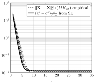
(a) $K_{a}=20,M=4$

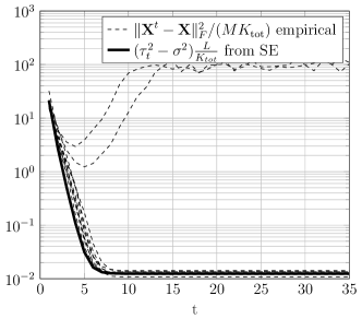
(b) $K_{a}=20,M=10$

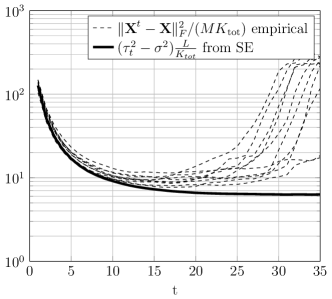
(c) $K_{a}=120,M=150$

Figure 1: Evolution of the normalized MSE in the AMP iterations (46)-(47) for 10 sample runs and its state evolution prediction from (52). $L=100$, $K_{\text{tot}}=2000$ and the LSFCs are chosen such that $\text{snr}_{k}$ (see (5)) are uniformly distributed between 0 and 20dB and are assumed to be known at the receiver.

IV-C Complexity Comparison

The complexity of the discussed covariance-based AD algorithms (ML and NNLS) scales with the size of the covariance matrix and the total number of users, i.e. $\mathcal{O}(K_{\text{tot}}L^{2})$, plus the complexity of once calculating the empirical covariance matrix which is linear in $ML$.

The complexity of MMV-AMP in each iteration scales like $\mathcal{O}(M^{2}LK_{\text{tot}})$ or, with a sub-sampled FFT matrix as pilot matrix, like $\mathcal{O}(M^{2}K_{\text{tot}}\log K_{\text{tot}})$. Using the simplified derivative as described in paragraph IV-B2 the complexity is reduced to $\min(\mathcal{O}(MK_{\text{tot}}\log K_{\text{tot}}),\mathcal{O}(MK_{\text{tot}}L))$. In any case the covariance-based algorithms scale better with $M$, while MMV-AMP scales better with $L$.

IV-D Scaling

The performance of AD is visualized in Figure 2 (‘CS regime’, i.e. $K_{a}\leq L$) and Figure 3 ($K_{a}>L$). Here we assumed all the LSFCs to be identically equal to 1, MMV-AMP was run with the full knowledge of the LSFCs and the ML and NNLS algorithms were run with the box-constraints described in Section III-C1. In Figure 2 the NNLS algorithm is comparably worse than MMV-AMP and ML. This is to be expected, since $M$ is small compared to $L$, which leads to a significant gap between the true and the empirical covariance matrix $\|\widehat{\boldsymbol{\Sigma}}_{\bf y}-\boldsymbol{\Sigma}_{\bf y}\|_{F}$. Interestingly, although the ML algorithm is also covariance based, it still outperforms MMV-AMP. In Figure 3 we see that beyond the CS regime, the performance of MMV-AMP significantly deteriorates, while the activity detection error probability of ML and NNLS still decays exponentially with $M$. In Figure 4 we compare the LSFC estimation performance of the ML and NNLS algorithms. The simulations confirms Corollary 2 and show that the relative $\ell_{1}$ recovery error of NNLS indeed decays like $1/\sqrt{M}$. We see that the same decay behavior holds for the ML algorithm only with significantly better constants. Note, that the number of required antennas for the ML algorithm scales fundamentally different depending on whether $K_{a}\leq L$ or $K_{a}>L$. In the first case the probability of error decays a lot faster with increasing $M$, matching qualitatively the scaling derived in Theorem 1, which states that (up to constant or logarithmic factors) $M=\mathcal{O}((K_{a}/L)^{2})$.

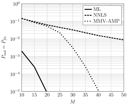
Figure 2: Scaling of the support detection error vs. $M$ at the border of the CS regime for $K_{a}=L=100,K_{\text{tot}}=2000$ with constant LSFCs at ${\mathsf{snr}}_{k}=0$ dB.

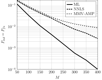
Figure 3: Scaling of the support detection error vs. $M$ beyond the CS regime (i.e. $K_{a}>L$). Here $K_{a}=300,L=100,K_{\text{tot}}=2000$ with constant LSFCs at ${\mathsf{snr}}_{k}=0$ dB.

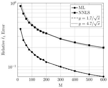
Figure 4: Relative $\ell_{1}$ error of the estimation of the LSFCs of the active users for $D_{c}=100,K_{a}=200,K_{\text{tot}}=2000$. The LSFCs are chosen such that ${\mathsf{snr}}_{k}$ are uniform in the range 0-20dB. The dotted lines show that the curves are well represented by a $c/\sqrt{M}$ behavior, for some constant $c$, as predicted by Corollary 2.

Corollary 2 predicts that, in the limit $M\to\infty$, the recovery error of NNLS vanishes, as long as the number of active users fulfils condition (15). We confirm this behavior empirically in Figure 5a, where we solve the NNLS problem (26) using the true covariance matrix $\boldsymbol{\Sigma}^{\circ}={\bf A}{\text{diag}}({\boldsymbol{\gamma}}^{\circ}){\bf A}^{{\sf H}}+\sigma^{2}{\bf I}_{L}$ instead of the empirical covariance matrix $\widehat{\boldsymbol{\Sigma}}_{\bf y}$. In this case, $\|{\bf d}\|_{2}=0$ in (33) and the recovery error should be identically zero when the true vector $\hbox{\boldmath$\gamma$}^{\circ}$ is $K_{a}$-sparse and the system parameters are such that Theorem 3 holds. This is confirmed by Figure 5a, showing a quadratic curve, below which the recovery error vanishes.

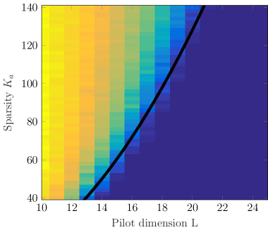
(a) ML

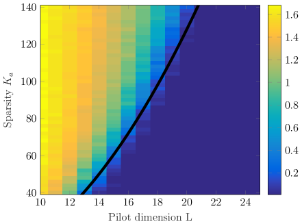
(b) NNLS

Figure 5: Phase transition of the recovery error for NNLS and ML in the limit $M\to\infty$ for $K_{\text{tot}}=1000$. The function $x\rightarrow(x-4)^{2}/2$ is overlayed in black to emphasize the super-linear scaling. The color indicates the normalized $\ell_{1}$-error as it is subject of Corollary 2 in the NNLS case. The LSFC are constant and the activity pattern is chosen uniformly at random from all $K_{a}$-sparse vectors. The results are obtained by averaging over random pilot matrices and activity patterns.

We also observe a very similar behavior for the ML algorithm, (see Figure 5b). This suggests that the condition (26) is indeed necessary independent of the algorithm.

Figure 6 shows the gain in performance when the LSFCs are known at the receiver and the box-constraint (step 8 in Algorithm 1) is employed.

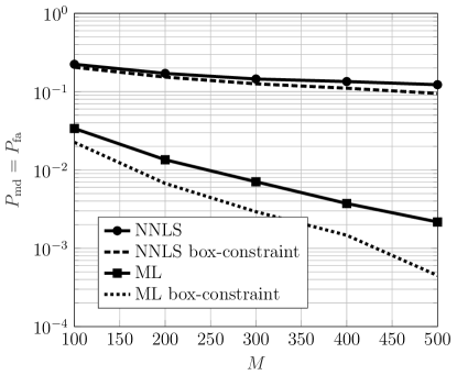
Figure 6: Effect of using the box-constraint (see step 8 in Algorithm 1) when the LSFCs $g_{k}$ are known at the receiver. Here $K_{a}=150,L=100,K_{\text{tot}}=2000$ and the LSFCs are distributed such that ${\mathsf{snr}}_{k}$ are uniform in the range $0-20$dB.

V Application: Massive MIMO Unsourced Random Access

As an application of the presented non-Bayesian algorithms and their analysis, in this section we introduce an extension of the recently posed unsourced random access problem [7] to the case of a massive MIMO BS receiver and show that the ML scheme (see Algorithm 1) provides an efficient low-complexity approach. The presented scaling properties in Corollary 41 enable us to estimate the required per-user-power, in terms of $E_{b}/N_{0}$, and the required number of receive antennas $M$ for reliable transmission.

The channel model is the same as described in Section II-A, i.e., a block-fading channel with blocks of $L$ signal dimensions over which the user channel vectors are constant. We assume $n=SL$, for some integer $S$, such that the transmission of a codeword spans $S$ fading blocks. Following the problem formulation in [7], each user is given the same codebook ${\cal C}=\{{\bf c}(m):m\in[2^{nR}]\}$, formed by $2^{nR}$ codewords ${\bf c}(m)\in\mathbb{C}^{n}$. A fixed but unknown number $K_{a}$ of users transmit their messages over the coherence block. The BS must then produce a list ${\cal L}$ of the transmitted messages $\{m_{k}:k\in{\cal K}_{a}\}$ (i.e., the messages of the active users). The system performance is expressed in terms of the Per-User Probability of Misdetection, defined as the average fraction of transmitted messages not contained in the list, i.e.,

$$p^{\text{msg}}_{\text{md}}=\frac{1}{K_{a}}\sum_{k\in\mathcal{K}_{a}}\mathbb{P}(m_{k}\notin\mathcal{L}),$$ (60)

and the Probability of False-Alarm, defined as the average fraction of decoded messages that were indeed not sent, i.e.,

$$p^{\text{msg}}_{\text{fa}}=\frac{|\mathcal{L}\setminus\{m_{k}:k\in{\cal K}_{a}\}|}{|\mathcal{L}|}.$$ (61)

The size of the list is also an outcome of the decoding algorithm, and therefore it is a random variable. As customary, the average error probabilities of false-alarm/misdetection are defined as the expected values of $p^{\text{msg}}_{\text{fa}}/p^{\text{msg}}_{\text{md}}$ resp. over all involved random variables. That is in this case the Rayleigh fading coefficients, the AWGN noise and the choice of messages, where the messages are assumed to be chosen uniformly and independent of each other. Notice, that in this problem formulation the total number of users $K_{\rm tot}$ is completely irrelevant, as long as it is much larger than the number of active user $K_{a}$ (e.g., we may consider $K_{\rm tot}=\infty$). Letting the average energy per symbol of the codebook ${\cal C}$ be denoted by $E_{s}=\frac{1}{n2^{nR}}\sum_{m=1}^{2^{nR}}\|{\bf c}(m)\|_{2}^{2}$, the received signal can be re-normalized such that the AWGN per-component variance is $\sigma^{2}=N_{0}/E_{s}$ and the received energy per code symbol is 1. In this way, the notation introduced for the AD model in (3) is preserved. Furthermore, as customary in coded systems, we express energy efficiency in terms of the standard quantity $E_{b}/N_{0}:=\frac{E_{s}}{RN_{0}}$.

V-A Unsourced random access as AD problem

For now assume $S=1$, i.e. each user transmits his codeword in a single block of length $L$. Further fix $J=LR$ and let ${\bf A}\in\mathbb{C}^{L\times 2^{J}}=[{\bf a}_{1},...,{\bf a}_{2^{J}}]$, be a matrix with columns normalized such that $\|{\bf a}_{i}\|_{2}^{2}=L$. Each column of ${\bf A}$ represents one codeword. Let $i_{k}$ denote the $J$-bit messages produced by the active users $k\in{\cal K}_{a}$, represented as integers in $[1:2^{J}]$, user $k$ simply sends the column ${\bf a}_{i_{k}}$ of the coding matrix ${\bf A}$. The received signal at the $M$-antennas BS takes on the form

$${\bf Y} = \sum_{k\in{\cal K}_{a}}\sqrt{g_{k}}{\bf a}_{i_{k}}{\bf h}^{\sf T}_{k}+{\bf Z}$$ (62)

$$= {\bf A}\boldsymbol{\Phi}{\bf G}^{1/2}{\bf H}+{\bf Z}$$

where, as for the AD model in (4), ${\bf G}={\text{diag}}(g_{1},\ldots,g_{K_{\rm tot}})$ is the diagonal matrix of LSFCs, ${\bf H}\in\mathbb{C}^{K_{\rm tot}\times M}$ is the matrix containing, by rows, the user channel vectors ${\bf h}_{k}$ formed by the small-scale fading antenna coefficients (Gaussian i.i.d. entries $\sim{\cal C}{\cal N}(0,1)$), ${\bf Z}\in\mathbb{C}^{L\times M}$ is the matrix of AWGN samples (i.i.d. entries $\sim{\cal C}{\cal N}(0,\sigma^{2})$), and $\boldsymbol{\Phi}\in\{0,1\}^{2^{J}\times K_{\rm tot}}$ is a binary selection matrix where for each $k\in{\cal K}_{a}$ the corresponding column $\boldsymbol{\Phi}_{:,k}$ is all-zero but a single one in position $i_{k}$, and for all $k\in{\cal K}_{\rm tot}\setminus{\cal K}_{a}$ the corresponding column $\boldsymbol{\Phi}_{:,k}$ contains all zeros.

Let’s focus on the matrix ${\bf X}=\boldsymbol{\Phi}{\bf G}^{1/2}{\bf H}$ of dimension $2^{J}\times M$. The $r$-th row of such matrix is given by

$${\bf X}_{r,:}=\sum_{k\in\mathcal{K}_{a}}\sqrt{g_{k}}\phi_{r,k}{\bf h}^{\sf T}_{k},$$ (63)

where $\phi_{r,k}$ is the $(r,k)$-th element of $\boldsymbol{\Phi}$, equal to one if $r=i_{k}$ and zero otherwise. It follows that ${\bf X}_{r,:}$ is Gaussian with i.i.d. entries $\sim{\cal C}{\cal N}\left(0,\sum_{k\in{\cal K}_{a}}g_{k}\phi_{r,k}\right)$. Since the messages are uniformly distributed over $[1:2^{J}]$ and statistically independent across the users, the probability that ${\bf X}_{r,:}$ is identically zero is given by $(1-2^{-J})^{K_{a}}$. Hence, for $2^{J}$ significantly larger than $K_{a}$, the matrix ${\bf X}$ is row-sparse.

In order to map the decoding into a problem completely analogous to the AD problem already discussed before, with some abuse of notation we define the modified LSFC-activity coefficients $\gamma_{r}:=\sum_{k\in\mathcal{K}_{a}}g_{k}\phi_{r,k}$ and $\boldsymbol{\Gamma}=\text{diag}(\gamma_{1},...,\gamma_{2^{J}})$. Then, (62) can be written as

$${\bf Y}={\bf A}\boldsymbol{\Gamma}^{1/2}\widetilde{{\bf H}}+{\bf Z},$$ (64)

where $\widetilde{{\bf H}}\in\mathbb{C}^{2^{J}\times M}$ with i.i.d. elements $\sim{\cal C}{\cal N}(0,1)$. Notice that in (64) the number of total users $K_{\rm tot}$ plays no role. In fact, none of the matrices involved in (64) depends on $K_{\rm tot}$.

The task of the inner decoder at the BS is to identify the non-zero elements of the modified active LSFC pattern $\gamma$, the vector of diagonal coefficients of $\boldsymbol{\Gamma}$. The active (non-zero) elements correspond to the indices of the transmitted messages. Notice that even if two or more users choose the same sub-message, the corresponding modified LSFC $\gamma_{r}$ is positive since it corresponds to the sum of the signal powers. In other words, since the detection scheme is completely non-coherent (it never explicitly estimates the complex channel matrix) and active signals add in power, there is no risk of signal cancellation or destructive interference.

At this point, it is clear that the problem of identifying the set of transmitted messages from observation (64) is completely analogous to the AD problem from the observation in (4), where the role of the total number of users $K_{\rm tot}$ in the AD problem is replaced by the number of messages $2^{J}$ in the inner decoding problem. Building on this analogy, we shall use the discussed ML algorithm to decode the inner code.

It is interesting to notice that the modified LSFCs in $\gamma$ are random sums of the individual user channel gains $\{g_{k}\}$. Hence, even if the $g_{k}$’s were exactly individually known, or their statistics was known, these random sums would have unknown values and unknown statistics (unless averaging over all possible active subsets, which would involve an exponential complexity in $K_{\rm tot}$ which is clearly infeasible in our context). Hence, Bayesian approaches such as MMV-AMP (see Section IV-B) as advocated in [12, 15, 64, 10] do not find a straightforward application here. In contrast, the proposed non-Bayesian approaches (in particular, the ML algorithm in Algorithm 1), that treats $\gamma$ as a deterministically unknown vector.

Notice also that in a practical unsourced random access scenario such as a large-scale IoT application, the slot dimension $L$ may be of the order of 100 to 200 symbols, while for a city-wide IoT data collector it is not unreasonable to have $M$ of the order of 500 to 1000 antennas (especially when considering narrowband signals such as in LoRA-type applications [65, 66]). This is precisely the regime where we have observed a critical behavior of MMV-AMP, while our algorithm uniformly improves as $M$ increases, for any slot dimension $L$.

V-B Discussion and analysis

In this section we discuss the performance of the ML decoder in a single slot ($S=1$). For the sake of simplicity, in the discussion of this section we assume $g_{k}=1$ for all $k$. In this case, the SNR $E_{s}/N_{0}$ is also the SNR at the receiver, for each individual (active) user.

Corollary 2 shows that, if the coding matrix ${\bf A}$ is chosen randomly, the probability of an error in the estimation of the support of $\gamma$ vanishes in the limit $M\to\infty$ for any SNR $\frac{E_{s}}{N_{0}}>0$ as long as $K_{a}=\mathcal{O}(L^{2}/\log^{2}(e2^{J}/L^{2}))$. Then Corollary 2 gives the following bound for the reconstruction error of

$$\frac{\lVert\hbox{\boldmath$\gamma$}-\hbox{\boldmath$\gamma$}^{*}\rVert_{1}}{\|\hbox{\boldmath$\gamma$}\|_{1}}\leq\kappa\left(1+\left(K_{a}\frac{E_{s}}{N_{0}}\right)^{-1}\right)\sqrt{\frac{K_{a}}{M}}$$ (65)

where $\kappa$ is some universal constant and $\hbox{\boldmath$\gamma$}^{*}$ denotes the estimate of $\gamma$ by the NNLS algorithm (see section III-B). Our numerical results (section IV-D) suggest that the reconstruction error of the ML algorithm is at least as good as that of NNLS (in practice it is typically much better). This bound is indeed very conservative. Nevertheless, this is enough to give achievable scaling laws for the probability of error of the inner decoder. It follows from (65) that $\frac{\lVert\hbox{\boldmath$\gamma$}-\hbox{\boldmath$\gamma$}^{*}\rVert_{1}}{\|\hbox{\boldmath$\gamma$}\|_{1}}\to 0$ for $(M,K_{a},\frac{E_{s}}{N_{0}})\to(\infty,\infty,0)$ as long as

$$\frac{K_{a}(1+(K_{a}E_{s}/N_{0})^{-1})^{2}}{M}=o(1),$$ (66)

which is satisfied if $M$ grows as

$$M=\max(K_{a},(E_{s}/N_{0})^{-1})^{\kappa}$$ (67)

for some $\kappa>1$. Assuming that $J$ scales such that $2^{J}=\delta L^{2}$ for some fixed $\delta\geq 1$, i.e. $J=\mathcal{O}(\log L)$, then the condition in Corollary 2 becomes $K_{a}=\mathcal{O}(L^{2})$ and we can conclude that the recovery error vanishes for sum spectral efficiencies up to

$$\frac{K_{a}J}{L}=\mathcal{O}(L\log L).$$ (68)

This shows that we can achieve a total spectral efficiency that grows without bound, by encoding over larger and larger blocks of dimension $L$, as long as the number of messages per user and the number of active users both grow proportionally to $L^{2}$ and the number of BS antennas scales as in (67). The achievable sum spectral efficiency grows as $L\log(L)$ and the error probability can be made as small as desired, for any given $E_{b}/N_{0}>0$. Of course, in this regime the rate per active user vanishes as $\log(L)/L$.

We wish to stress again that this system is completely non-coherent, i.e., there is no attempt to either explicitly (via pilot symbols) or implicitly to estimate the channel matrix (small-scale fading coefficients).

V-C Reducing complexity via concatenated coding

In practice it is not feasible to transmit even small messages (e.g. $J\sim 100$) within one coherence block ($S=1$), because the number of columns of the coding matrix ${\bf A}$ grows exponentially in $J$. Aside from the computational complexity $L$ may also be limited physically by the coherence time of the channel. In both cases it is necessary to transmit the message over multiple blocks. Let each user transmit his message over a frame of $S$ fading blocks and within each block use the code described in section V-A as inner code with the ML decoder as inner decoder.

We follow the concatenated coding scheme approach of [45], suitably adapted to our case. Let $B=nR$ denote the number of bits per user message. For some suitable integers $S\geq 1$ and $J>0$, we divide the $B$-bit message into blocks of size $b_{1},b_{2},\ldots,b_{S}$ such that $\sum_{s}b_{s}=B$ and such that $b_{1}=J$ and $b_{s}<J$ for all $s=2,\ldots,S$. Each subblock $s=2,3,\ldots,S$ is augmented to size $J$ by appending $p_{s}=J-b_{s}$ parity bits, obtained using pseudo-random linear combinations of the information bits of the previous blocks $s^{\prime}<s$. Therefore, there is a one-to-one association between the set of all sequences of coded blocks and the paths of a tree of depth $S$. The pseudo-random parity-check equations generating the parity bits are identical for all users, i.e., each user makes use exactly of the same outer tree code. For more details on the outer coding scheme, please refer to [45].

Given $J$ and the slot length $L$, the inner code is used to transmit in sequence the $S$ (outer-encoded) blocks forming a frame. Let ${\bf A}$ be the coding matrix as defined in section V-A. Each column of ${\bf A}$ now represents one inner codeword. Letting $i_{k}(1),\ldots,i_{k}(S)$ denote the sequence of $S$ (outer-)encoded $J$-bit messages produced by the outer encoder of active user $k\in{\cal K}_{a}$. The user $k$ now simply sends in sequence, over consecutive slots of length $L$, the columns ${\bf a}_{i_{k}(1)},{\bf a}_{i_{k}(2)},...,{\bf a}_{i_{k}(S)}$ of the coding matrix ${\bf A}$. As described in section V-A, the inner decoding problem is equivalent to the AD problem (64). For each subslot $s$, let $\widehat{\hbox{\boldmath$\gamma$}}[s]=(\widehat{\gamma}_{1}[s],\ldots,\widehat{\gamma}_{2^{J}}[s])^{\sf T}$ denote the ML estimate of $\gamma$ in subslot $s$ obtained by the inner decoder. Then, the list of active messages at subslot $s$ is defined as

$${\cal S}_{s}=\left\{r\in[2^{J}]:\widehat{\gamma}_{r}[s]\geq\nu_{s}\right\},$$ (69)

where $\nu_{1},\ldots,\nu_{S}$ are suitable pre-defined thresholds. Let ${\cal S}_{1},{\cal S}_{2},\ldots,{\cal S}_{S}$ the sequence of lists of active subblock messages. Since the subblocks contain parity bits with parity profile $\{0,p_{2},\ldots,p_{S}\}$, not all message sequences in ${\cal S}_{1}\times{\cal S}_{2}\times\cdots\times{\cal S}_{S}$ are possible. The role of the outer decoder is to identify all possible message sequences, i.e., those corresponding to paths in the tree of the outer tree code [45]. The output list ${\cal L}$ is initialized as an empty list. Starting from $s=1$ and proceeding in order, the decoder converts the integer indices ${\cal S}_{s}$ back to their binary representation, separates data and parity bits, computes the parity checks for all the combinations with messages from the list ${\cal L}$ and extends only the paths in the tree which fulfill the parity checks. A precise analysis of the error probability of such a decoder and its complexity in terms of surviving paths in the list is given in [45]. The performance of the concatenated system is demonstrated via simulations in the following section.

V-D Asymptotic analysis - Outer code

We define the support $\hbox{\boldmath$\rho$}[s]$ of the estimated $\widehat{\hbox{\boldmath$\gamma$}}[s]$ as a binary vector whose $r$-th element is equal to 1 if $\widehat{\gamma}_{r}[s]\geq\nu_{s}$ and to zero otherwise. In the case of error-free support recovery, $\hbox{\boldmath$\rho$}[s]$ can be interpreted as the output of a vector “OR” multiple access channel (OR-MAC) where the inputs are the binary columns of the activity matrix $\boldsymbol{\Phi}[s]$ and the output is given by

$$\hbox{\boldmath$\rho$}[s]=\bigvee_{k\in{\cal K}_{a}}\boldsymbol{\Phi}_{:,k}[s],$$ (70)

where $\bigvee$ denotes the component-wise binary OR operation. The logical “OR” arises from the fact that if the same sub-message is selected by multiple users, it will show up as “active” at the output of the “activity-detection” inner decoder since the signal energy adds up (as discussed before). Classical code constructions for the OR-MAC, like [67, 68], have been focussed on zero-error decoding, which does not allow for positive per-user-rates as $K_{a}\to\infty$, see e.g. [69] for a recent survey. Capacity bounds for the OR-MAC under the given input constraint have been derived in [70] and [71], where it was called the “T-user M-frequency noiseless MAC without intensity information”” or “A-channel””. An asynchronous version of this channel was studied in [72]. Note, that the capacity bounds in the literature are combinatorial and hard to evaluate numerically for large numbers of $K_{a}$ and $2^{J}$. In the following we will show that, in the typical case of $K_{a}\ll 2^{J}$, a simple upper bound on the achievable rates based on the componentwise entropy is already tight because it is achievable by the outer code of [45].

V-D1 Achievability

The analysis in [45] shows that the error probability of the outer code goes to zero in the so called logarithmic regime with constant outer rate, i.e. for $K_{a},J\to\infty$ as $J=\alpha\log_{2}K_{a}$ and $B=SR_{\text{out}}J$ if the number of parity bits $P$ is chosen as ([45, Theorem 5 and 6])

1. $P=(S+\delta-1)\log_{2}K_{a}$ for some constant $\delta>0$ if all the parity bits are allocated in the last slots.

2. $P=c(S-1)\log_{2}K_{a}$ for some constant $c>1$ if the parity bits are allocated evenly at the end of each subslot except for the first.

In the first case the complexity scales like $\mathcal{O}(K_{a}^{R_{\text{out}}S}\log K_{a})$, since there is no pruning in the first $R_{\text{out}}S$ subslots, while in the second case the complexity scales linearly with $S$ like $\mathcal{O}(SK_{a}\log K_{a})$. The corresponding outer rates are

$$\begin{split}R_{\text{out}}&=B/(B+P)\\ &=1-P/(B+P)\\ &=1-P/(SJ)\\ &=1-\frac{S+\delta-1}{S\alpha}\\ &=1-\frac{1}{\alpha}+\frac{1}{S}\frac{\delta-1}{\alpha}\end{split}$$ (71)

for the case of all parity bits in the last sections and

$$\begin{split}R_{\text{out}}&=1-\frac{c(S-1)}{S\alpha}\\ &=1-\frac{c}{\alpha}-\frac{c}{S\alpha}\end{split}$$ (72)

for the case of equally distributed parity bits. In the limit $S\to\infty$ the achievable rates are therefore $R_{\text{out}}=1-1/\alpha$ and $R_{\text{out}}=1-c/\alpha$ respectively.

V-D2 Converse

The output entropy of the vector OR-MAC of dimension $2^{J}$ is bounded by the entropy of $2^{J}$ scalar OR-MACs. The marginal distribution of the entries of $\hbox{\boldmath$\rho$}[s]$ is Bernoulli with $\mathbb{P}(\rho_{r}[s]=0)=(1-2^{-J})^{K_{a}}$. Hence, we have

$$H(\rho[s])\leq 2^{J}{\cal H}_{2}((1-2^{-J})^{K_{a}}).$$ (73)

We stay in the logarithmic scaling regime, introduced in the previous sections, i.e. we fix $J=\alpha\log_{2}K_{a}$ for some $\alpha>1$ and consider the limit $K_{a},J\to\infty$. In this regime $K_{a}/2^{J}=K_{a}^{-(\alpha-1)}\to 0$ and we have $1-(1-2^{-J})^{K_{a}}=K_{a}/2^{J}+\mathcal{O}((K_{a}/2^{J})^{2})\to 0$. This gives that

$$2^{J}{\cal H}_{2}((1-2^{-J})^{K_{a}})\to K_{a}(J-\log_{2}K_{a})=(\alpha-1)K_{a}\log_{2}K_{a}.$$ (74)

Since all users make use of the same code we have that the number of information bits sent by the $K_{a}$ active users over a slot is $B_{\text{sum}}=K_{a}JR_{\text{out}}$. Therefore, in order to hope for small probability of error a necessary condition is

$$K_{a}JR_{\text{out}}\leq 2^{J}\mathcal{H}_{2}((1-1/2^{J})^{K_{a}}).$$ (75)

So the outer rate is limited by

$$R_{\text{out}}\leq(\alpha-1)\frac{\log_{2}K_{a}}{J}=1-\frac{1}{\alpha}.$$ (76)

We have shown in the previous Section V-D1 that this outer rate can be achieved in the limit of infinite subslots $S\to\infty$ by the described outer tree code at the cost of a decoding complexity of at least $\mathcal{O}(K_{a}^{R_{\text{out}}S})$ or up to a constant factor $\Delta R_{\text{out}}=(c-1)/\alpha$ for some $c>1$ with a complexity of $\mathcal{O}(SK_{a}\log K_{a})$. This is a noteworthy results on its own, since it is a priori not clear, whether the bound (75) is achievable by an unsourced random access scheme, i.e. each user using the same codebook.
The resulting achievable sum spectral efficiency can be calculated as in section V-B with a subtle but important difference, since the results on the outer code are valid only in the logarithmic regime $J=\alpha\log_{2}K_{a}$, i.e. $2^{J}=K_{a}^{\alpha}$ for $\alpha>1$. According to Corollary 2 the error probability of the inner code vanishes if the number of active users scale no faster then $K_{a}=\mathcal{O}(L^{2}/\log^{2}(e2^{J}/L^{2}))$. Using the scaling condition $J=\alpha\log_{2}K_{a}$ and that $K_{a}\leq L^{2}$, this implies that in the logarithmic regime the error probability of the inner code vanishes if the number of active users scales as $K_{a}=\mathcal{O}(L^{2}/\log^{2}(L))$. This gives a sum spectral efficiency of

$$\frac{K_{a}R_{\text{out}}J}{L}=\mathcal{O}\left(\frac{K_{a}\log K_{a}}{L}\right)=\mathcal{O}\left(\frac{L}{\log L}\right).$$ (77)

The order of this sum spectral efficiency is, by a factor $\log^{2}L$, smaller then the one we calculated in section V-B. This is because the order of supported active users is smaller by exactly the same $\log^{2}L$ factor. In section V-B we assumed that $J$ scales as $2^{J}=\delta L^{2}=\mathcal{O}(K_{a})$ for some $\delta>1$, so that the ratio $K_{a}/2^{J}$ remains constant. It is not clear from the analysis in [45], whether the probability of error of the outer tree code would vanish in the regime. We can get a converse by evaluating the entropy bound (75). Let $2^{J}=\delta K_{a}$ with $\delta>1$, then $(1-2^{-J})^{K_{a}}=(1-\delta/K_{a})^{K_{a}}\xrightarrow[K_{a}\to\infty]{}\exp(-\delta)$. Therefore the binary entropy ${\cal H}_{2}((1-2^{-J})^{K_{a}})$ remains a constant in the limit $J,K_{a}\to\infty$ and we get that

$$K_{a}R_{\text{out}}J\leq\delta K_{a}{\cal H}_{2}(\exp(-\delta)).$$ (78)

This shows that $R_{\text{out}}\to 0$ in the limit $J,K_{a}\to\infty$ is the best achievable asymptotic per-user outer rate, but the outer sum rate $K_{a}R_{\text{out}}J$ is proportional to $K_{a}$. The resulting sum spectral efficiencies scale as

$$\frac{K_{a}R_{\text{out}}J}{L}=\mathcal{O}\left(\frac{K_{a}}{L}\right)=\mathcal{O}(L).$$ (79)

This means it could be possible to increase the achievable sum spectral efficiencies by a factor of $\log L$ by using an outer code that is able to achieve the entropy bound (75) in the regime $2^{J}=\delta K_{a}$. It is not clear though whether the code of [45] or some other code can achieve this.

V-E Simulations

The outer decoder requires a hard decision on the support of the estimated $\widehat{\hbox{\boldmath$\gamma$}}[s]$. When $K_{a}$ is known, one approach consists of selecting the $K_{a}+\Delta$ largest entries in each section, where $\Delta\geq 0$ can be adjusted to balance between false alarm and misdetection in the outer channel. However, the knowledge of $K_{a}$ is a very restrictive assumption in such type of systems. An alternative approach, which does not require this knowledge, consists of fixing a sequence of thresholds $\{\nu_{s}:s\in[S]\}$ and let $\hbox{\boldmath$\rho$}[s]$ to be the binary vector of dimension $2^{J}$ with elements equal to 1 for all components of $\widehat{\hbox{\boldmath$\gamma$}}[s]$ above threshold $\nu_{s}$. By choosing the thresholds, we can balance between missed detections and false alarms. Furthermore, we may consider the use of a non-uniform decaying power allocation across the slots as described in [73].

For the simulations in Figure 7 we choose $B=96$ bits as payload size for each user, a frame of $S=32$ slots of $L=100$ dimensions per slot, yielding an overall block length $n=3200$. Choosing the binary subblock length $J=12$, the inner coding matrix ${\bf A}$ has dimension $100\times 4096$ and therefore is still quite manageable. We choose the columns of ${\bf A}$ uniformly i.i.d. from the sphere of radius $\sqrt{L}$. For the outer code, we choose the following parity profile $p=[0,9,9,\ldots,9,12,12,12]$, yielding an outer coding rate $R_{out}=0.25$ information bits per binary symbol. Notice also that if one wishes to send the same payload message using the piggybacking scheme of [64, 10], each user should make use of $2^{96}$ columns, which is totally impractical. All large scale fading coefficients are fixed to $g_{k}\equiv 1$. In Figure 7 we fix $N_{0}=1$ and choose the transmit power (energy per symbol), such that $E_{b}/N_{0}=0$dB and plot the sum of the two types of error probabilities $P_{e}=p^{\text{msg}}_{\text{md}}+p^{\text{msg}}_{\text{fa}}$, (see (60) and (61)) as a function of the number of active users for different numbers of receive antennas $M$. Figure 8 shows how $P_{e}$ falls as a function of $E_{b}/N_{0}$ for different values of $K_{a}$ and $M$. Figure 9 shows the required values of $E_{b}/N_{0}$ as a function of $K_{a}$ to achieve a total error probability $P_{e}<0.05$ for the code parameters in Table I. We use three different settings here, depending on the values of the coherence block-length $L$. In all three the total block-length is fixed to $n=3200$ and $B\approx 100$, which gives a per-user spectral efficiency of $R\approx 0.031$ bits per channel use. With $K_{a}=300$ this corresponds to a total spectral efficiency $\mu\approx 9$ bits per channel use, which is significantly larger than today’s LTE cellular systems (in terms of bit/s/Hz per sector) and definitely much larger than IoT-driven schemes such as LoRA [65, 66]. The simulations confirm qualitatively the behavior predicted in Sections V-B and V-D. The achievable total spectral efficiencies seem to be mainly limited by the coherence block-length $L$, and for a given total spectral efficiency the required energy-per-bit can be made arbitrary small by increasing $M$. According to the Shannon-limit for the scalar Gaussian multiple access channel (only one receive antenna, no fading) $E_{b}/N_{0}>(2^{K_{a}R}-1)/(K_{a}R)$, and therefore one needs at least $\approx 17.5$ dB to achieve a total spectral efficiency of $9$ bits per channel use. Here we find that gains of $20$ dB or more are possible even with non-coherent detection by the use of multiple receive antennas. This shows also quantitatively that the non-coherent massive MIMO channel is very attractive for unsourced random access, since it preserves the same desirable characteristics of unsourced random access as in the non-fading Gaussian model of [7] (users transmit without any pre-negotiation, and no use of pilot symbols is needed), while the total spectral efficiency can be made as large as desired simply by increasing the number of receiver antennas.

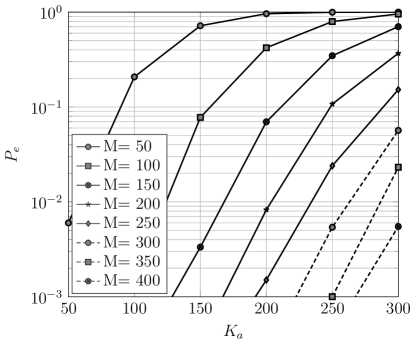
Figure 7: Error probability ($P_{e}=p^{\text{msg}}_{\text{md}}+p^{\text{msg}}_{\text{fa}}$) as a function of the number of active users for different numbers of receive antennas. $E_{b}/N_{0}=$ 0 dB, $L=100$, $n=3200$, $B=96$ bits, $S=32,J=12$.

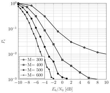
(a) $K_{a}=300$

(b) $M=300$

Figure 8: Error probability ($P_{e}=p^{\text{msg}}_{\text{md}}+p^{\text{msg}}_{\text{fa}}$) as a function of $E_{b}/N_{0}$. $L=100$, $n=3200$, $b=96$ bits, $S=32,J=12$.

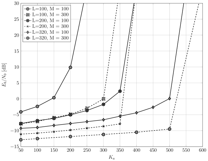
Figure 9: Required energy-per-bit to achieve $P_{e}<0.05$. $L$ and $S$ are varied, while $n=3200$ and $B\approx 100$ are fixed. The precise parameters are given in Table I.

	S	J	$R_{\text{out}}$	Parity profile	B
$L=100$	32	12	0.25	[0,9,…,9,12,12,12]	96
$L=200$	16	15	0.42	[0,7,8,8,9,…,9,13,14]	100
$L=320$	10	19	0.52	[0,9,…,9,19]	99

TABLE I: Parameters for Figure 9

VI Conclusion

In this paper, we studied the problem of user activity detection in a massive MIMO setup, where the BS has $M\gg 1$ antennas. We showed that with a coherence block containing $L$ signal dimensions one can reliably estimate the activity of $K_{a}=O(L^{2}/\log^{2}(K_{\rm tot}/K_{a}))$ active users in a set of $K_{\rm tot}$ users, which is a much larger than the previous bound $K_{a}=O(L)$ obtained via traditional compressed sensing techniques. In particular, in our proposed scheme one needs to pay only a poly-logarithmic penalty $O(\log^{2}(K_{\rm tot}/K_{a}))$ with respect to the number of potential users $K_{\rm tot}$, which makes the scheme ideally suited for activity detection in IoT setups where the number of potential users can be very large. We discuss low-complexity algorithms for activity detection and provided numerical simulations to illustrate our results and compared them with approximated message passing schemes recently proposed for the same scenario. In particular, as a byproduct of our numerical investigation, we also showed a curious unstable behavior of MMV-AMP in the regime where the number of receiver antennas is large, which is precisely the case of interest with a massive MIMO receiver. Finally, we proposed a scheme for unsourced random access where all users make use of the same codebook and the receiver task is to come up with the list of transmitted messages. We use our activity detection scheme(s) directly, where now the users’ signature sequences play the role of codewords, and the number of total users plays the role of the number of total messages. We showed that an arbitrarily fixed probability of error can be achieved at any $E_{b}/N_{0}$ for sufficiently large number of antennas, and a total spectral efficiency that grows as $O(L\log L)$, where $L$ is the code block length, can be achieved. Such one-shot scheme is conceptually nice but not suited for typical practical applications with message payload of the order of $B\approx 100$ bits, since it would require a codebook matrix with $2^{B}$ columns. Hence, we have also considered the application of the concatenated approach pioneered in [45], where the message is broken into a sequence of smaller blocks and the activity detection scheme is applied as an inner encoding/decoding stage at each block, while an outer tree code takes care of “stitching together” the sequence of decoded submessages over the blocks. Numerical simulations show the effectiveness of the proposed method. It should be noticed that these schemes are completely non-coherent, i.e., the receiver never tries to estimate the massive MIMO channel matrix of complex fading coefficients. Therefore, the scheme pays no hidden penalty in terms of pilot symbol overhead, often connected with the assumption of ideal coherent reception, i.e., channel state information known to the receiver.

Appendix A Proof of Theorem 1

The main line of arguments in this section is based on [38]. In turns, the proof in [38] is based on a RIP result which was claimed and successively retracted [39]. The result was applied to a non-centered matrix and therefore could not have the claimed property. We fix this here, using our own new RIP result (Theorem 2) and, for the sake of clarity and self-contained presentation, give a complete streamlined proof for the case of known LSFCs. At several points our proof technique differs from [38], which results in the slightly better bound on $M$. Let us first introduce some notation.

Definition 1

For $t>1$ define the Renyi divergence of order $t$ between two probability densities $p$ and $q$ as

$$\mathcal{D}_{t}(p,q):=\frac{1}{t-1}\ln\int p(x)^{t}q(x)^{1-t}\mathrm{d}x$$ (80)

$\lozenge$

Definition 2

A differentiable function $f$ is called strongly convex with parameter $m>0$ if the following inequality holds for all points $x,y$ in its domain:

$$f(y)\geq f(x)+\nabla f(x)^{\top}(y-x)+\frac{m}{2}\|x-y\|^{2}_{2}$$ (81)

$\lozenge$

Let ${\bf b}^{\circ}$ denote the true activity pattern with known sparsity $K_{a}$, and ${\bf b}^{*}$ be the output of the estimator (12). Using the union bound, we can write

$$\begin{split}\mathbb{P}({\bf b}^{*}\neq{\bf b}^{\circ})&=\mathbb{P}\left(\max_{{\bf b}\in\Theta_{K_{a}}\setminus\{{\bf b}^{\circ}\}}p({\bf Y}|{\bf b})\geq p({\bf Y}|{\bf b}^{\circ})\right)\\ &=\mathbb{P}\left(\bigcup_{{\bf b}\in\Theta_{K_{a}}\setminus\{{\bf b}^{\circ}\}}\{p({\bf Y}|{\bf b})\geq p({\bf Y}|{\bf b}^{\circ})\}\right)\\ &\leq\sum_{{\bf b}\in\Theta_{K_{a}}\setminus\{{\bf b}^{\circ}\}}\mathbb{P}({\bf Y}:p({\bf Y}|{\bf b})-p({\bf Y}|{\bf b}^{\circ})\geq 0)\\ &\leq\sum_{{\bf b}\in\Theta_{K_{a}}\setminus\{{\bf b}^{\circ}\}}\mathbb{P}({\bf Y}:p({\bf Y}|{\bf b})-p({\bf Y}|{\bf b}^{\circ})>-\alpha)\end{split}$$ (82)

for any $\alpha>0$. With slight abuse of notation we define $\boldsymbol{\Sigma}({\bf b}):={\bf A}{\bf B}{\bf G}^{\circ}{\bf A}^{{\sf H}}+\sigma^{2}{\bf I}_{L}$, the covariance matrix for a given binary pattern ${\bf b}$ for a fixed vector of LSFCs ${\bf g}^{\circ}$, with ${\bf B}={\text{diag}}({\bf b})$ and ${\bf G}^{\circ}={\text{diag}}({\bf g}^{\circ})$. Let $p_{\bf b}:=\mathcal{CN}(0,\boldsymbol{\Sigma}({\bf b}))$ denote the Gaussian distribution with covariance matrix $\boldsymbol{\Sigma}({\bf b})$, then $\log p({\bf Y}|{\bf b})=\sum_{j}\log p_{\bf b}({\bf Y}_{:,j})$. The following large deviation property of $\log p({\bf Y}|{\bf b})$ is established in [38, Corollary 1]:

Theorem 4

$$\begin{split}&\mathbb{P}\left(\log p({\bf Y}|{\bf b})-\log p({\bf Y}|{\bf b}^{\circ})>-\frac{M}{2}\mathcal{D}_{1/2}(p_{\bf b},p_{{\bf b}^{\circ}})\right)\\ &\leq\exp\left(-\frac{M}{4}\mathcal{D}_{1/2}(p_{\bf b},p_{{\bf b}^{\circ}})\right)\end{split}$$ (83)

where $\mathcal{D}_{1/2}(p_{\bf b},p_{{\bf b}^{\circ}})$ is the Renyi divergence of order $1/2$ between $p_{\bf b}$ and $p_{\bf b}^{\circ}$ defined in Definition 1. $\square$

The result of Theorem 4 holds only if $\mathcal{D}_{1/2}(p_{\bf b},p_{{\bf b}^{\circ}})>0$, so in the following we will establish conditions under which this is true. First, note that since $p_{\bf b}$ and $p_{{\bf b}^{\circ}}$ are zero-mean Gaussian distributions with covariance matrices $\boldsymbol{\Sigma}({\bf b})$ and $\boldsymbol{\Sigma}({\bf b}^{\circ})$ resp., their Renyi divergence of order $t$ can be expressed in closed form as:

$$\mathcal{D}_{t}(p_{\bf b},p_{{\bf b}^{\circ}})=\frac{1}{2(1-t)}\log\frac{|(1-t)\boldsymbol{\Sigma}({\bf b})+t\boldsymbol{\Sigma}({\bf b}^{\circ})|}{|\boldsymbol{\Sigma}({\bf b})|^{1-t}|\boldsymbol{\Sigma}({\bf b}^{\circ})|^{t}}$$ (84)

Let $\psi({\bf b}):=-\log|\boldsymbol{\Sigma}({\bf b})|$, then we can see that $\mathcal{D}_{t}(p_{\bf b},p_{{\bf b}^{\circ}})\geq t\frac{m^{*}}{4}\|{\bf b}-{\bf b}^{\circ}\|_{2}^{2}$, with $m^{*}$ being the strong convexity constant of $\psi(\cdot)$, is equivalent to

$$\psi((1-t){\bf b}+t{\bf b}^{\circ})\leq(1-t)\psi({\bf b})+t\psi({\bf b}^{\circ})-\frac{1}{2}m^{*}t(1-t)\|{\bf b}-{\bf b}^{\circ}\|_{2}^{2}.$$ (85)

Here we used the fact that

$$\begin{split}-\psi((1-t){\bf b}+t{\bf b}^{\circ})&=\log|\boldsymbol{\Sigma}((1-t){\bf b}+t{\bf b}^{\circ})|\\ &=\log|{\bf A}((1-t){\bf B}+t{\bf B}^{\circ}){\bf G}^{\circ}{\bf A}^{{\sf H}}+\sigma^{2}{\bf I}_{L}|\\ &=\log|(1-t)\boldsymbol{\Sigma}({\bf b})+t\boldsymbol{\Sigma}({\bf b}^{\circ})|\end{split}$$ (86)

Inequality (85) is precisely the condition that $\psi(\cdot)$ is strongly convex along the line connecting ${\bf b}$ and ${\bf b}^{\circ}$. So if $\psi(\cdot)$ is strongly convex on the set of $2K_{a}$-sparse vectors, then

$$\mathcal{D}_{t}(p_{\bf b},p_{{\bf b}^{\circ}})\geq t\frac{m^{*}}{4}\|{\bf b}-{\bf b}^{\circ}\|_{2}^{2}$$ (87)

holds for any $K_{a}$-sparse vectors ${\bf b}$ and ${\bf b}^{\circ}$. Let ${\bf b}_{1},{\bf b}_{2}\in\Theta_{K_{a}}$ be two arbitrary $K_{a}$-sparse vectors. Since $\log|\cdot|$ is differentiable on $\mathbb{R}^{+}$, a Taylor expansion of $\psi({\bf b}_{1})$ around ${\bf b}_{2}$ gives:

$$\begin{split}\psi({\bf b}_{1})=\psi({\bf b}_{2})&+\langle\nabla\psi({\bf b}_{1}),{\bf b}_{2}-{\bf b}_{1}\rangle\\ &+\frac{1}{2}({\bf b}_{2}-{\bf b}_{1})^{\top}\nabla^{2}\psi({\bf b}_{r})({\bf b}_{2}-{\bf b}_{1})\end{split}$$ (88)

for ${\bf b}_{r}=(1-r){\bf b}_{1}+r{\bf b}_{2}$ with some $r\in[0,1]$. Let $\Delta{\bf b}:={\bf b}_{2}-{\bf b}_{1}$, then the strong convexity of $\psi(\cdot)$ is equivalent to

$$\sum_{i,j}\left.\frac{\partial\psi}{\partial b_{i}\partial b_{j}}\right|_{{\bf b}={\bf b}_{r}}\Delta b_{i}\Delta b_{j}\geq m^{*}\|{\bf b}_{2}-{\bf b}_{1}\|_{2}^{2}.$$ (89)

The derivatives of $\psi$ are given by:

$$\left.\frac{\partial\psi}{\partial b_{i}}\right|_{{\bf b}={\bf b}_{r}}=-\mathsf{tr}(\boldsymbol{\Sigma}({\bf b}_{r})^{-1}g_{i}^{\circ}{\bf a}_{i}{\bf a}_{i}^{{\sf H}})$$ (90)

$$\left.\frac{\partial\psi}{\partial b_{i}\partial b_{j}}\right|_{{\bf b}={\bf b}_{r}}=\mathsf{tr}(\boldsymbol{\Sigma}({\bf b}_{r})^{-1}g_{i}^{\circ}{\bf a}_{i}{\bf a}_{i}^{{\sf H}}\boldsymbol{\Sigma}({\bf b}_{r})^{-1}g_{j}^{\circ}{\bf a}_{j}{\bf a}_{j}^{{\sf H}})$$ (91)

Next we will calculate $m^{*}$. It holds that

$$\begin{split}\sum_{i,j}\left.\frac{\partial\psi}{\partial b_{i}\partial b_{j}}\right|_{{\bf b}={\bf b}_{r}}\Delta b_{i}\Delta b_{j}&=\sum_{i,j}\mathsf{tr}\left(\boldsymbol{\Sigma}({\bf b}_{r})^{-1}\Delta b_{i}g_{i}^{\circ}{\bf a}_{i}{\bf a}_{i}^{{\sf H}}\boldsymbol{\Sigma}({\bf b}_{r})^{-1}\Delta b_{j}g_{j}^{\circ}{\bf a}_{j}{\bf a}_{j}^{{\sf H}}\right)\\ &=\mathsf{tr}\left(\boldsymbol{\Sigma}({\bf b}_{r})^{-1}\left(\sum_{i}\Delta b_{i}g_{i}^{\circ}{\bf a}_{i}{\bf a}_{i}^{{\sf H}}\right)\boldsymbol{\Sigma}({\bf b}_{r})^{-1}\left(\sum_{j}\Delta b_{j}g_{j}^{\circ}{\bf a}_{j}{\bf a}_{j}^{{\sf H}}\right)\right)\\ &=\mathsf{tr}\left(\boldsymbol{\Sigma}({\bf b}_{r})^{-1}(\boldsymbol{\Sigma}({\bf b}_{2})-\boldsymbol{\Sigma}({\bf b}_{1}))\boldsymbol{\Sigma}({\bf b}_{r})^{-1}(\boldsymbol{\Sigma}({\bf b}_{2})-\boldsymbol{\Sigma}({\bf b}_{1}))\right)\\ &\geq\sigma_{\text{min}}(\boldsymbol{\Sigma}({\bf b}_{r})^{-1})\mathsf{tr}\left((\boldsymbol{\Sigma}({\bf b}_{2})-\boldsymbol{\Sigma}({\bf b}_{1}))\boldsymbol{\Sigma}({\bf b}_{r})^{-1}(\boldsymbol{\Sigma}({\bf b}_{2})-\boldsymbol{\Sigma}({\bf b}_{1}))\right)\\ &\geq\sigma^{2}_{\text{min}}(\boldsymbol{\Sigma}({\bf b}_{r})^{-1})\|\boldsymbol{\Sigma}({\bf b}_{2})-\boldsymbol{\Sigma}({\bf b}_{1})\|_{F}^{2}\\ &=\frac{\|\boldsymbol{\Sigma}({\bf b}_{2})-\boldsymbol{\Sigma}({\bf b}_{1})\|_{F}^{2}}{\sigma^{2}_{\text{max}}(\boldsymbol{\Sigma}({\bf b}_{r}))}.\end{split}$$ (92)

Here $\sigma_{\text{min}}({\bf A})$ (resp., $\sigma_{\text{max}}({\bf A})$) denotes the minimum (resp., maximum) singular value of ${\bf A}$. In the first and the second inequality in (92) we used the fact that $\mathsf{tr}({\bf A}{\bf B})\geq\sigma_{\text{min}}({\bf A})\mathsf{tr}({\bf B})$ for positive semi-definite matrices ${\bf A},{\bf B}$, and in the second inequality in (92) we used the fact that the covariance matrix is symmetric and $\mathsf{tr}({\bf A}^{\top}{\bf A})=\|{\bf A}\|_{F}^{2}$.

We can rewrite $\|\boldsymbol{\Sigma}({\bf b}_{2})-\boldsymbol{\Sigma}({\bf b}_{1})\|_{F}^{2}=\|{\mathbb{A}}({\bf g}^{\circ}\odot({\bf b}_{2}-{\bf b}_{1}))\|_{2}^{2}$, where ${\mathbb{A}}\in\mathbb{C}^{L^{2}\times K_{\text{tot}}}$ is the matrix defined in (27), obtained by stacking the $L^{2}$-dimensional vectors $\text{vec}({\bf a}_{k}{\bf a}_{k}^{{\sf H}})$ by columns. We show in (156) that $\|{\mathbb{A}}{\bf x}\|_{2}\geq\|\mathring{{\mathbb{A}}}{\bf x}\|_{2}$ holds $\forall{\bf x}\in\mathbb{R}^{K_{\text{tot}}}$, with $\mathring{{\mathbb{A}}}$ being the centered version of ${\mathbb{A}}$, which is defined in (29).

We show in Theorem 2, that, with probability at least $1-\exp(-c_{\delta}L)$, $\mathring{{\mathbb{A}}}/\sqrt{L(L-1)}$, the centered and rescaled version of ${\mathbb{A}}$ has RIP of order $2K_{a}$ with constant $\delta_{2K_{a}}<\delta$ if condition (13) is fulfilled. In particular $\|\mathring{{\mathbb{A}}}{\bf x}\|_{2}^{2}\geq(1-\delta_{2K_{a}})L(L-1)\|{\bf x}\|_{2}^{2}$ holds for all $2K_{a}$-sparse vectors ${\bf x}$. So the RIP of $\mathring{{\mathbb{A}}}$ implies that

$$\begin{split}\|\boldsymbol{\Sigma}({\bf b}_{2})-\boldsymbol{\Sigma}({\bf b}_{1})\|_{F}^{2}&\geq(1-\delta_{2K_{a}})L(L-1)\|{\bf g}^{\circ}\odot({\bf b}_{2}-{\bf b}_{1})\|_{2}^{2}\\ &\geq(1-\delta_{2K_{a}})L(L-1)g_{\text{min}}^{2}\|{\bf b}_{2}-{\bf b}_{1}\|_{2}^{2}\\ &\geq\frac{1}{2}(1-\delta_{2K_{a}})L^{2}g_{\text{min}}^{2}\|{\bf b}_{2}-{\bf b}_{1}\|_{2}^{2}\end{split}$$ (93)

An upper bound on $\sigma_{\text{max}}^{2}(\boldsymbol{\Sigma}({\bf b}_{r}))=\|\boldsymbol{\Sigma}({\bf b}_{r})\|_{op}^{2}$ can be found as follows. Note that for any binary $2K_{a}$-sparse vector ${\bf b}$, it holds that

$$\begin{split}\sigma_{\text{max}}(\boldsymbol{\Sigma}({\bf b}))&=\|\boldsymbol{\Sigma}({\bf b})\|_{op}\\ &=\left\|\sum_{k=1}^{K_{\text{tot}}}g^{\circ}_{k}b_{k}{\bf a}_{k}{\bf a}_{k}^{{\sf H}}+\sigma^{2}{\bf I}\right\|_{op}\\ &\leq g_{\text{max}}\left\|\sum_{k\in{\rm supp\,}({\bf b})}{\bf a}_{k}{\bf a}_{k}^{{\sf H}}\right\|_{op}+\sigma^{2}\\ &=g_{\text{max}}\left\|\sum_{k\in{\rm supp\,}({\bf b})}({\bf a}_{k}{\bf a}_{k}^{{\sf H}}-{\bf I})+2K_{a}{\bf I}\right\|_{op}+\sigma^{2}\\ &\leq g_{\text{max}}\left\|\sum_{k\in{\rm supp\,}({\bf b})}({\bf a}_{k}{\bf a}_{k}^{{\sf H}}-{\bf I})\right\|_{op}+g_{\text{max}}2K_{a}+\sigma^{2}\end{split}$$ (94)

Now $\sum_{k\in{\rm supp\,}({\bf b})}({\bf a}_{k}{\bf a}_{k}^{{\sf H}}-{\bf I})$ is a sum of $2K_{a}$ random matrices ${\bf a}_{k}{\bf a}_{k}^{{\sf H}}$, with ${\bf a}_{k}$ drawn i.i.d. from the sphere of radius $\sqrt{L}$, and therefore sub-Gaussian. A generic large deviation result for such matrices, e.g., the complex version of [74, Theorem 4.6.1], shows that

$$\left\|\sum_{k\in{\rm supp\,}({\bf b})}({\bf a}_{k}{\bf a}_{k}^{{\sf H}}-{\bf I})\right\|_{op}\leq\left(\sqrt{K_{a}}+C\left(\sqrt{L}+t\right)\right)^{2}$$ (95)

holds with probability at least $1-2\exp(-t^{2})$ for some universal constant $C>0$. Let $t=\sqrt{\beta}\max(\sqrt{K_{a}},\sqrt{L})$ for some $\beta>0$. Then (94) gives that

$$\sigma_{\text{max}}(\boldsymbol{\Sigma}({\boldsymbol{\gamma}}))\leq(1+\beta C^{\prime})g_{\text{max}}\max\{K_{a},L\}+\sigma^{2}$$ (96)

holds with probability at least $1-\exp(-\beta\max\{K_{a},L\})$ for some universal constants $C^{\prime}>0$. So (92) can be further bounded using (93) and (96) as

$$\frac{\|\boldsymbol{\Sigma}({\bf b}_{2})-\boldsymbol{\Sigma}({\bf b}_{1})\|_{F}^{2}}{\sigma^{2}_{\text{max}}(\boldsymbol{\Sigma}({\bf b}_{r}))}\geq\frac{(1-\delta_{2K_{a}})g_{\text{min}}^{2}\|{\bf b}_{2}-{\bf b}_{1}\|_{2}^{2}}{2\left((1+C^{\prime}\beta)g_{\text{max}}\max\left\{\frac{K_{a}}{L},1\right\}+\frac{\sigma^{2}}{L}\right)^{2}}$$ (97)

Together with (89) and (92) this implies that, if the pilot matrix satisfies the RIP of order $2K_{a}$ with constant $\delta_{2K_{a}}<1$, then $\psi(\cdot)$ is strongly convex along the line between any two $K_{a}$-sparse vectors with constant

$$m^{*}\geq\frac{(1-\delta_{2K_{a}})g_{\text{min}}^{2}}{2\left((1+C^{\prime}\beta)g_{\text{max}}\max\left\{\frac{K_{a}}{L},1\right\}+\frac{\sigma^{2}}{L}\right)^{2}}$$ (98)

with probability exceeding $1-\exp(-\beta\max\{K_{a},L\})$. Since the bound is independent of the chosen vectors and the number of $2K_{a}$ sparse binary vectors is bounded by $\binom{K_{\text{tot}}}{2K_{a}}\leq(eK_{\text{tot}}/K_{a})^{2K_{a}}\leq(eK_{\text{tot}}/K_{a})^{2\max\{K_{a},L\}}$, (98) holds in the set of all $2K_{a}$-sparse vectors with probability exceeding

$$1-\exp\left(-2\max\{K_{a},L\}\left(\frac{\beta}{2}-\log\left(\frac{eK_{\text{tot}}}{2K_{a}}\right)\right)\right)$$ (99)

This probability exceeds $1-\epsilon$ if

$$\beta\geq 2\log\left(\frac{eK_{\text{tot}}}{2K_{a}}\right)+\frac{\log(2/\epsilon)}{\max\{K_{a},L\}}$$ (100)

We get that

$$\begin{split}m^{*}\geq\frac{(1-\delta_{2K_{a}})g_{\text{min}}^{2}}{2\left(C^{\prime}\left(2\log\left(\frac{eK_{\text{tot}}}{2K_{a}}\right)+\frac{\log(2/\epsilon)}{\max\{K_{a},L\}}\right)g_{\text{max}}\max\left\{\frac{K_{a}}{L},1\right\}+\frac{\sigma^{2}}{L}\right)^{2}}\end{split}$$ (101)

holds with probability exceeding $1-\epsilon$.

Let $k_{d}=\|{\bf b}_{2}-{\bf b}_{1}\|_{0}\leq 2K_{a}$ denote the number of positions in which ${\bf b}_{2}$ and ${\bf b}_{1}$ differ, i.e. their Hamming distance. Then the Renyi divergence (87) can be lower bound as:

$$\mathcal{D}_{t}(p_{\bf b},p_{{\bf b}^{\circ}})\geq t\frac{m^{*}}{4}k_{d}$$ (102)

Putting everything together, we can complete the union bound. Note that there are $\binom{K_{a}}{k_{d}}\binom{K_{\text{tot}}-K_{a}}{k_{d}}\leq(3eK_{\text{tot}}K_{a})^{k_{d}}$ ways to choose a support which differs from the true support in $k_{d}$ positions. Now, denote by $\mathcal{C}$ the event that the pilot matrix ${\bf A}$ is such that the RIP condition (93) holds, and the bound (101). Using (82), Theorem 4 and (102) we get that

$$\begin{split}\mathbb{P}({\bf b}^{*}\neq{\bf b}^{\circ},\mathcal{C})&\leq\sum_{{\bf b}\in\Theta_{K_{a}}\setminus\{{\bf b}^{\circ}\}}\exp\left(-\frac{M}{4}\mathcal{D}_{1/2}(p_{\bf b},p_{{\bf b}^{\circ}})\right)\\ &\leq\sum_{k_{d}=1}^{2K_{a}}(3eK_{\text{tot}}K_{a})^{k_{d}}\exp\left(-M\frac{m^{*}}{4}k_{d}\right)\\ &=\sum_{k_{d}=1}^{2K_{a}}\exp\left(-k_{d}\left(M\frac{m^{*}}{4}-\log(3eK_{\text{tot}}K_{a})\right)\right)\end{split}$$ (103)

So let

$$M\geq\frac{4}{m^{*}}\log\left(3eK_{\text{tot}}K_{a}\frac{1+\epsilon}{\epsilon}\right)$$ (104)

which is precisely condition (14), then

$$\begin{split}\mathbb{P}({\bf b}^{*}\neq{\bf b}^{\circ},\mathcal{C})&\leq\sum_{k_{d}=1}^{2K_{a}}\left(\frac{\epsilon}{1+\epsilon}\right)^{k_{d}}\\ &\leq\epsilon\end{split}$$ (105)

Finally

$$\begin{split}\mathbb{P}({\bf b}^{*}\neq{\bf b}^{\circ})&\leq\mathbb{P}({\bf b}^{*}\neq{\bf b}^{\circ},\mathcal{C})+\mathbb{P}(\bar{\mathcal{C}})\\ &\leq\epsilon+\epsilon+\exp(-C_{\delta}L)\end{split}$$ (106)

This concludes the proof of Theorem 1.

Appendix B Proof of the RIP, Theorem 2

Let us first define some basic properties.

Definition 3 (Sub-Exponential Norm)

Let $X$ be a real scalar random variable. Define the sub-exponential norm of $X$ as

$$\|X\|_{\psi_{1}}:=\inf\left\{t>0:\mathbb{E}\left[\exp\left(\frac{|X|}{t}\right)\right]\leq 2\right\}.$$ (107)

A well known property of sub-exponential variables is that

$$\mathbb{P}(|X|>t)\leq 2\exp(-ct/\|X\|_{\psi_{1}})\quad\forall t>0$$ (108)

for some universal constant $c>0$.

Definition 4 (Sub-Exponential Random Vector)

Let ${\bf X}$ be a random vector in $\mathbb{R}^{n}$. ${\bf X}$ is said to be sub-exponential if all its marginals are scalar sub-exponential random variables, i.e. if

$$\sup_{{\bf x}\in S^{n-1}}\|\langle{\bf X},{\bf x}\rangle\|_{\psi_{1}}<\infty$$ (109)

then we define $\|{\bf X}\|_{\psi_{1}}:=\sup_{{\bf x}\in S^{n-1}}\|\langle{\bf X},{\bf x}\rangle\|_{\psi_{1}}$, where $S^{n-1}$ is the unit sphere in $\mathbb{R}^{n}$.

Basic properties of sub-exponential random variables and vectors can be found e.g. in Ch. 2 and 3 of [74].

Definition 5 (Convex Concentration Property (2.2 in [75]))

Let ${\bf X}$ be a random vector in $\mathbb{R}^{n}$. ${\bf X}$ has the convex concentration property with constant $K$ if for every 1-Lipschitz convex function $\phi:\mathbb{R}^{n}\to\mathbb{R}$, we have $\mathbb{E}[|\phi({\bf X})|]<\infty$ and for every $t>0$,

$$\mathbb{P}(|\phi({\bf X})-\mathbb{E}[\phi({\bf X})]|\geq t)\leq 2\exp(-t^{2}/K^{2})$$ (110)

For the RIP of $\mathring{{\mathbb{A}}}/\sqrt{m}$ we first establish the following results for generic matrices ${\bf R}\in\mathbb{R}^{m\times N}$ with independent normalized columns.

Theorem 5

Let ${\bf R}\in\mathbb{R}^{m\times N}$ be a matrix with independent columns ${\bf R}_{:,i}$ normalized such that $\mathbb{E}[\|{\bf R}_{:,i}\|_{2}^{2}]=m$, with $\psi_{1}$-norm at most $\psi$. Furthermore, assume that the distribution of the columns satsifies

$$\mathbb{P}(|\|{\bf R}_{:,i}\|_{2}^{2}-m|>tm)\leq\exp(-c\sqrt{m})$$ (111)

for some constant $c>0$. Also assume that $N\geq m$ and $\sqrt{m}>c^{\prime}\log 4N$ for some universal constant $c^{\prime}>0$. Then the RIP constant of ${\bf R}/\sqrt{m}$ satisfies $\delta_{2s}({\bf R}/\sqrt{m})<\delta$ with probability $\geq 1-\exp(-C^{\prime}\sqrt{c_{\delta,\xi}m})$ for

$$2s=c_{\delta,\xi}\frac{m}{\log^{2}(eN/c_{\delta,\xi}m)},$$ (112)

where $c_{\delta,\xi}\leq\min\{1,\frac{\delta^{2}}{(3C\xi^{2})^{2}}\}$ for any $\xi>\psi+1$ and $C,C^{\prime}>0$ are universal constants. $\square$

Proof:

We make use of the following generic RIP result from [50, Theorem 3.3] for matrices with i.i.d. sub-exponential columns:

Theorem 6

Let $m\geq 1$ and $s,N$ be integers such that $1\leq s\leq\min(N,m)$. Let ${\bf R}_{:,1},...,{\bf R}_{:,N}\in\mathbb{R}^{m}$ be independent sub-exponential random vectors normalized such that $\mathbb{E}[\|{\bf R}_{:,i}\|^{2}]=m$ and let $\psi=\max_{i\leq N}\|{\bf R}_{:,i}\|_{\psi_{1}}$. Let $\theta^{\prime}\in(0,1)$, $K,K^{\prime}\geq 1$ and set $\xi=\psi K+K^{\prime}$. Then for the matrix ${\bf R}$ with columns ${\bf R}_{:,i}$

$$\delta_{s}\left(\frac{{\bf R}}{\sqrt{m}}\right)\leq C\xi^{2}\sqrt{\frac{s}{m}}\log\left(\frac{eN}{s\sqrt{\frac{s}{m}}}\right)+\theta^{\prime}$$ (113)

holds with probability larger than

$$\begin{split}1&-\exp\left(-\hat{c}K\sqrt{s}\log\left(\frac{eN}{s\sqrt{\frac{s}{m}}}\right)\right)\\ &-\mathbb{P}\left(\max_{i\leq N}\|{\bf R}_{:,i}\|_{2}\geq K^{\prime}\sqrt{m}\right)-\mathbb{P}\left(\max_{i\leq N}\left|\frac{\|{\bf R}_{:,i}\|_{2}^{2}}{m}-1\right|\geq\theta^{\prime}\right),\end{split}$$ (114)

where $C,\hat{c}>0$ are universal constants. $\square$

In order to prove Theorem 5 we shall apply Theorem 6. Let us abbreviate $\delta_{s}=\delta_{s}\left(\frac{{\bf R}}{\sqrt{m}}\right)$. We set $\theta^{\prime}=\delta_{s}/2$ and Therefore, we consider the bound

$$\delta_{s}\leq C\xi^{2}\sqrt{\frac{s}{m}}\log\left(\frac{eN}{s\sqrt{s/m}}\right)=:D,$$ (115)

that holds with probability larger than (114). Let $s=cm/\log^{2}(e\frac{N}{cm})$ for any $0<c\leq 1$. Note that the conditions $c\leq 1$ and $N\geq m$ guarantee that $\log(e\frac{N}{cm})\geq 1$. Plugging into (115) we see that the RIP-constant satisfies

$$\delta_{s} \leq C\xi^{2}\sqrt{c}\frac{\log(e(\frac{N}{cm})^{3/2}\log^{3}(e\frac{N}{cm}))}{\log(e\frac{N}{cm})}$$ (116)

$$\leq C\xi^{2}\sqrt{c}\left(\frac{3}{2}+\frac{3\log\log e\frac{N}{cm}}{\log e\frac{N}{cm}}\right)$$ (117)

$$\leq C\xi^{2}\sqrt{c}\left(\frac{3}{2}+\frac{3}{e}\right)$$ (118)

$$\leq 3C\xi^{2}\sqrt{c}$$ (119)

where in the first line we made use of $m\leq N$ and in the last line we used $\log\log x/\log x\leq 1/e$. We proceed to bound the probability in (114). Using the union bound, the last two terms in (114) can be bound as:

$$\mathbb{P}\left(\max_{i\leq N}\|{\bf R}_{:,i}\|_{2}\geq K^{\prime}\sqrt{m}\right) \leq N\mathbb{P}\left(\|{\bf R}_{:,i}\|^{2}_{2}\geq K^{\prime 2}m\right)$$ (120)

$$\leq N\mathbb{P}\left(|\|{\bf R}_{:,i}\|^{2}_{2}-m|\geq(K^{\prime 2}-1)m\right)$$ (121)

and

$$\mathbb{P}\left(\max_{i\leq N}\left|\frac{\|{\bf R}_{:,i}\|_{2}^{2}}{m}-1\right|\geq\theta^{\prime}\right) \leq N\mathbb{P}\left(|\|{\bf R}_{:,i}\|^{2}_{2}-m|\geq\theta^{\prime}m\right)$$ (122)

By choosing $K^{\prime}=\sqrt{1+\theta}$ we can treat both terms equivalently. By the tail bound assumption on the norms we have

$$2N\mathbb{P}\left(|\|{\bf R}_{:,i}\|^{2}_{2}-m|\geq\theta^{\prime}m\right)\leq\exp(\log 4N-c\sqrt{m})\leq\exp(-c^{\prime}\sqrt{m})$$ (123)

for some positive constants $c,c^{\prime}$. The last inequality follows from the assumption $\sqrt{m}>c^{\prime}\log 4N$. Also we have

$$\exp\left(-\widehat{c}K\sqrt{s}\log\left(e\frac{N\sqrt{m}}{s^{3/2}}\right)\right) \leq\exp\left(-\widehat{c}K\sqrt{s}\log\left(e\frac{N}{m}\right)\right)$$ (124)

$$=\exp(-\widehat{c}K\sqrt{c}\sqrt{m})$$ (125)

where in the first line we used $s\leq m$. By choosing $c$ small enough such that $\hat{c}K\sqrt{c}\sqrt{m}<c^{\prime}$ we get from (123) and (125) that

$$\mathbb{P}(\delta_{s}>D)\leq 2\exp(-\widehat{c}K\sqrt{c}\sqrt{m})$$ (126)

The statement of Theorem 5 follows by choosing $c$ small enough such that $\delta_{s}\leq\delta$.     $\sqcap$$\sqcup$

We want to apply Theorem 5, which holds for real values matrices ${\bf R}$, to the matrix

$${\mathbb{A}}^{R}:=\sqrt{2}[{\rm Re}(\mathring{{\mathbb{A}}});{\rm Im}(\mathring{{\mathbb{A}}})]\in\mathbb{R}^{2L(L-1)\times{K_{\text{tot}}}},$$ (127)

i.e., the real matrix obtained by stacking real and imaginary part of $\mathring{{\mathbb{A}}}$, with $m=2L(L-1)$ and $N=K_{\text{tot}}$. Consider the $k$-th column ${\mathbb{A}}^{R}_{:,k}$ of ${\mathbb{A}}^{R}$. We have

$$\begin{split}\mathbb{E}\left[\|[{\rm Re}(\mathring{{\mathbb{A}}}_{:,k});{\rm Im}(\mathring{{\mathbb{A}}}_{:,k})]\|_{2}^{2}\right]/c_{L}&=\mathbb{E}\left[\|{\rm Re}(\mathring{{\mathbb{A}}}_{:,k})\|_{2}^{2}+\|{\rm Im}(\mathring{{\mathbb{A}}}_{:,k})\|^{2}_{2}\right]/c_{L}\\ &=\mathbb{E}\left[\|\mathring{{\mathbb{A}}}_{:,k}\|_{2}^{2}\right]/c_{L}\\ &=\mathbb{E}\left[\sum_{i\neq j}|a_{k,i}a_{k,j}^{{\sf H}}|^{2}\right]\\ &=\mathbb{E}\left[\left(\sum_{i=1}^{L}|a_{k,i}|^{2}\right)^{2}\right]-\sum_{i=1}^{L}\mathbb{E}[|a_{k,i}|^{4}]\\ &=L^{2}-L\kappa_{a}\\ &=L(L-\kappa_{a}),\end{split}$$ (128)

Since $c_{L}$ was chosen exactly as $(L-1)/(L-\kappa_{a})$ we have $\mathbb{E}[\|{\mathbb{A}}^{R}_{:,k}\|_{2}^{2}]=m$. Note that a spherical vector is especially sub-Gaussian, which implies that its fourth moment can be bound by a constant independent of the dimension [74]. To apply Theorem 5 we need to show that the columns of ${\mathbb{A}}^{R}$ are sub-exponential with $\psi_{1}$ norm independent of the dimension.

Note that for any vector ${\bf u}\in\mathbb{R}^{2L(L-1)}$ the marginal $\langle{\mathbb{A}}^{R}_{:,k},{\bf u}\rangle$ can be expressed as a quadratic form in ${{\bf a}_{k}^{R}:=\sqrt{2}[{\rm Re}({\bf a}_{k});{\rm Im}({\bf a}_{k})]}$ as the following calculation shows. Let ${\bf U},\widetilde{{\bf U}}\in\mathbb{R}^{L\times L}$ be two matrices with zeros on the diagonal such that ${\bf u}=[\text{vec}_{\text{non-diag}}({\bf U});\text{vec}_{\text{non-diag}}(\widetilde{{\bf U}})]$. Then it holds:

$$\begin{split}\left\langle{\mathbb{A}}^{R}_{:,k},{\bf u}\right\rangle&=\sqrt{2}\sum_{i\neq j}\left({\rm Re}(a_{k,i}a^{{\sf H}}_{k,j})U_{ij}+{\rm Im}(a_{k,i}a^{{\sf H}}_{k,j})\widetilde{U}_{ij}\right)\\ &=({\bf a}_{k}^{R})^{\top}{\bf Q}_{\bf u}{\bf a}^{R}_{k}\end{split}$$ (129)

with

$${\bf Q}_{\bf u}=\frac{1}{\sqrt{2}}\left(\begin{matrix}{\bf U}&\widetilde{{\bf U}}\\ -\widetilde{{\bf U}}&{\bf U}\end{matrix}\right)$$ (130)

and therefore $\|{\bf Q}_{\bf u}\|^{2}_{F}=\|{\bf u}\|^{2}_{2}$.
This form of ${\bf Q}_{\bf u}$ follows from the identities:

$${\rm Re}(a_{k,i}a_{k,j}^{{\sf H}}) ={\rm Re}(a_{k,i}){\rm Re}(a_{k,j})+{\rm Im}(a_{k,i}){\rm Im}(a_{k,j})$$ (131)

$${\rm Im}(a_{k,i}a_{k,j}^{{\sf H}}) =-{\rm Re}(a_{k,i}){\rm Im}(a_{k,j})+{\rm Im}(a_{k,i}){\rm Re}(a_{k,j})$$ (132)

We can now use the following concentration result for quadratic forms from [75] which states that a random vector which satisfies the convex concentration property also satisfies the following inequality, known as Hanson-Wright inequality [76]:

Theorem 7 (Theorem 2.5 in [75])

Let ${\bf X}$ be a mean zero random vector in $\mathbb{R}^{n}$, which satisfies the convex concentration property with constant $B$, then for any $n\times n$ matrix ${\bf Y}$ and every $t>0$,

$$\mathbb{P}(|{\bf X}^{\top}{\bf Y}{\bf X}-\mathbb{E}[{\bf X}^{\top}{\bf Y}{\bf X}]|>t)$$

$$\leq 2\exp\left(-c\min\left(\frac{t^{2}}{2B^{4}\|{\bf Y}\|_{F}^{2}},\frac{t}{B^{2}\|{\bf Y}\|_{op}}\right)\right)$$ (133)

$\square$.

Note that a random variable with such a mixed tail behavior is especially sub-exponential. This can be seen by bounding its moments. Let $Z$ be a random variable with

$$\mathbb{P}(|Z|>t)\leq 2\exp\left(-c\min\left(\frac{t^{2}}{B^{4}\|{\bf Y}\|_{F}^{2}},\frac{t}{B^{2}\|{\bf Y}\|_{op}}\right)\right)$$ (134)

Since $\|{\bf Y}\|_{op}\leq\|{\bf Y}\|_{F}$, we have $\mathbb{P}(|Z|>t)\leq 2\exp(-c\min(x(t)^{2},x(t)))$ for $x(t)=\frac{t}{B^{2}\|{\bf Y}\|_{F}}$. It follows

$$\begin{split}&\mathbb{E}[|Z|^{p}]=\int_{0}^{\infty}\mathbb{P}(|Z|^{p}>u)\mathrm{d}u=p\int_{0}^{\infty}\mathbb{P}(|Z|>t)t^{p-1}\mathrm{d}t\\ &\leq 2p(B^{2}\|Y\|_{op})^{p}\left(\int_{0}^{1}e^{-x^{2}}x^{p-1}\mathrm{d}x+\int_{1}^{\infty}e^{-x}x^{p-1}\mathrm{d}x\right)\\ &\leq 2p(B^{2}\|Y\|_{op})^{p}\left(\Gamma(p/2)+\Gamma(p)\right)\\ &\leq 4p(B^{2}\|Y\|_{op})^{p}\Gamma(p)\leq 4p(pB^{2}\|Y\|_{op})^{p}\end{split}$$ (135)

where $\Gamma(\cdot)$ is the Gamma function. So

$$(\mathbb{E}[|Z|^{p}])^{\frac{1}{p}}\leq(4p)^{\frac{1}{p}}pB^{2}\|{\bf Y}\|_{op}\leq cpB^{2}\|{\bf Y}\|_{op}$$ (136)

where $c=4e^{1/e}$. (136) is equivalent to $\|Z\|_{\psi_{1}}\leq cB^{2}\|{\bf Y}\|_{op}$ by elementary properties of sub-exponential random variables, e.g. [74, Proposition 2.7.1].

The convex concentration property was introduced in Definition 5. In our case the pilots ${\bf a}_{k}\in\mathbb{C}^{L}$ are distributed uniformly on the complex $L$-dimensional sphere of radius $L$, therefore the real versions ${\bf a}_{k}^{R}\in\mathbb{R}^{2L}$ are distributed uniformly on the sphere of radius $2L$. A classical result states that a spherical random variable ${\bf X}\sim\text{Unif}(\sqrt{n}S^{n-1})$ has the even stronger (non-convex) concentration property (e.g. [74, Theorem 5.1.4]):

Theorem 8 (Concentration on the Sphere)

Let ${\bf X}\sim\textup{Unif}(\sqrt{n}S^{n-1})$ be uniformly distributed on the Euclidean sphere of radius $\sqrt{n}$. Then there is an universal constant $c>0$, such that for every K-Lipschitz function $f:\sqrt{n}S^{n-1}\to\mathbb{R}$

$$\mathbb{P}(|f({\bf X})-\mathbb{E}[f({\bf X})]|>t)\leq 2\exp(-ct^{2}/K)$$ (137)

$\square$

So in particular the columns ${\bf a}_{k}^{R}$ have the convex concentration property with some constant $c>0$, independent of the dimension and it follows by (129) and Theorem 7 applied to ${\bf X}={\bf a}_{k}^{R}$ and ${\bf Y}={\bf Q}_{\bf u}$ that the marginals of $\langle{\mathbb{A}}^{R}_{:,k},{\bf u}\rangle$ uniformly satisfy the tail bound of the Hanson-Wright inequality. As shown in (136), this implies that the columns of ${\mathbb{A}}^{R}$ are sub-exponential with

$$\|{\mathbb{A}}^{R}_{:,k}\|_{\psi_{1}}=\max_{{\bf u}\in S^{2L(L-1)-1}}\|\langle{\mathbb{A}}^{R}_{:,k},{\bf u}\rangle\|_{\psi_{1}}\leq C$$ (138)

for some universal constant $C>0$. It remains to show the tail bound property (111). From the calculation in (128) we see that the column norms of ${\mathbb{A}}^{R}$ differ only in the term $f({\bf a}_{k}):=\sum_{i=1}^{L}|a_{k,i}|^{4}$, which is a $2\sqrt{L}$-Lipschitz function of the random vector ${\bf a}_{k}$ which satisfies the concentration property in Theorem 8. Substituting $t=tm$ and $K=2\sqrt{L}$ in Theorem 8 gives the desired tail bound. With this we can apply Theorem 5 and together with Theorems 7 and 8 it follows that ${\mathbb{A}}^{R}$, as defined in (127), has RIP of order $2s$ with RIP constant $\delta_{2s}({\mathbb{A}}^{R}/\sqrt{m})<\delta$ as long as

$$2s\leq C_{\delta}\frac{m}{\log^{2}(eK_{\text{tot}}/m)}.$$ (139)

Then, for the complex valued $\mathring{{\mathbb{A}}}$ it holds that

$$\left\|\frac{\mathring{{\mathbb{A}}}{\bf x}}{\sqrt{L(L-1)}}\right\|_{2}=\left\|\frac{\sqrt{2}[{\rm Re}(\mathring{{\mathbb{A}}});{\rm Im}(\mathring{{\mathbb{A}}})]{\bf x}}{\sqrt{2L(L-1)}}\right\|_{2}=\left\|\frac{{\mathbb{A}}^{R}{\bf x}}{\sqrt{m}}\right\|_{2}$$ (140)

for any ${\bf x}\in\mathbb{R}^{K_{\text{tot}}}$ and therefore the RIP of ${\mathbb{A}}^{R}/\sqrt{m}$ implies the RIP of $\mathring{{\mathbb{A}}}/\sqrt{L(L-1)}$ with the same constants, which concludes the proof of Theorem 2. Note that the constraint $\sqrt{m}>c^{\prime}\log 4N$ is naturally fulfilled when $m$ is large enough since an exponential scaling of $N$ would makes the achievable sparsity $s$ go to zero.

Appendix C Proof of the Recovery Guarantee for NNLS, Theorem 3

Throughout this section let ${\boldsymbol{\gamma}}^{*}$ denote the NNLS estimate

$${\boldsymbol{\gamma}}^{*}=\mathop{\rm arg\,min}_{{\boldsymbol{\gamma}}\in\mathbb{R}_{+}^{K_{\text{tot}}}}\|{\mathbb{A}}{\boldsymbol{\gamma}}-{\bf w}\|_{2}^{2}$$ (141)

as introduced in Section III-B, where ${\mathbb{A}}$ is the $L^{2}\times K_{\text{tot}}$ matrix whose $k$-th column is given by ${\rm vec}({\bf a}_{k}{\bf a}_{k}^{{\sf H}})$ and

$${\bf w}=\text{vec}(\widehat{\boldsymbol{\Sigma}}_{\bf y}-\sigma^{2}{\bf I}_{L}),$$ (142)

where $\widehat{\boldsymbol{\Sigma}}_{\bf y}$ is assumed to be the empirical covariance matrix (7) of $M$ iid samples from a Gaussian distribution $\mathcal{CN}(0,\boldsymbol{\Sigma}_{\bf y})$ with covariance matrix

$$\boldsymbol{\Sigma}_{\bf y}=\sum_{i=1}^{K_{\text{tot}}}\gamma_{k}^{\circ}{\bf a}_{k}{\bf a}_{k}^{{\sf H}}+\sigma^{2}{\bf I}_{L}$$ (143)

where ${\boldsymbol{\gamma}}^{\circ}=(\gamma^{\circ}_{1},\dots,\gamma^{\circ}_{K_{\text{tot}}})\in{\mathbb{R}}_{+}^{K_{\text{tot}}}$ is the true (unknown) activity pattern. So ${\bf w}$ can be expressed as

$${\bf w}={\mathbb{A}}{\boldsymbol{\gamma}}^{\circ}+{\bf d}$$ (144)

for ${\bf d}:=\text{vec}(\boldsymbol{\Sigma}_{\bf y}-\widehat{\boldsymbol{\Sigma}}_{\bf y})$. Let us introduce some notation.

Definition 6 (Robust NSP (4.21 in [37]))

${\mathbb{A}}\in\mathbb{C}^{L^{2}\times K_{\text{tot}}}$ is said to satisfy the robust $\ell_{q}$ nullspace property (NSP) of order $s$ with parameters $0<\rho<1$ and $\tau>0$ if

$$\lVert\mathbf{v}_{S}\rVert_{{q}}\leq\frac{\rho}{s^{1-1/q}}\lVert\mathbf{v}_{\bar{S}}\rVert_{{1}}+\tau\left\lVert{\mathbb{A}}\mathbf{v}\right\rVert_{{2}}\quad\forall\mathbf{v}\in\mathbb{R}^{K_{\text{tot}}}$$ (145)

holds for all subsets $S\subset[{K_{\text{tot}}}]$ with $|S|\leq s$. The set $\bar{S}$ denotes here the complement of $S$ in $[{K_{\text{tot}}}]$.

Furthermore let the $\ell_{1}$-error of the best $s$-sparse approximation to ${\boldsymbol{\gamma}}^{\circ}$ be denoted as:

$$\sigma_{s}({\boldsymbol{\gamma}}^{\circ})_{{1}}=\min_{\lVert{\boldsymbol{\gamma}}\rVert_{0}\leq s}\lVert{\boldsymbol{\gamma}}^{\circ}-{\boldsymbol{\gamma}}\rVert_{{1}}$$ (146)

If ${\boldsymbol{\gamma}}^{\circ}$ is assumed to actually be $s$-sparse, then we obviously have $\sigma_{s}({\boldsymbol{\gamma}}^{\circ})_{1}=0$. The statement of Theorem 3 will be an immediate consequence of the following theorem:

Theorem 9

If ${\mathbb{A}}\in\mathbb{C}^{L^{2}\times K_{\text{tot}}}$ has the robust $\ell_{2}$ NSP of order $s$ with constants $\tau>0$ and $\rho\in(0,1)$ and there exists a ${\bf t}\in\mathbb{C}^{K_{\text{tot}}}$, such that $\mathbf{1}={\mathbb{A}}^{{\sf H}}{\bf t}$, where $\mathbf{1}:=(1,...,1)^{\top}$, then for $p\in[1,2]$ the NNLS estimate ${\boldsymbol{\gamma}}^{*}$ in (141) satisfies

$$\|{\boldsymbol{\gamma}}^{*}-{\boldsymbol{\gamma}}^{\circ}\|_{p}\leq\frac{2C\sigma_{s}({\boldsymbol{\gamma}}^{\circ})_{{1}}}{s^{1-1/p}}+\frac{2D}{s^{\frac{1}{2}-\frac{1}{p}}}\left(\tau+\frac{\|{\bf t}\|_{2}}{s^{\frac{1}{2}}}\right)\|\mathbf{d}\|_{{2}}$$ (147)

with $C\coloneqq\frac{(1+\rho)^{2}}{1-\rho}$, $D=\frac{(3+\rho)}{1-\rho}$ and ${\bf d}=\text{vec}(\boldsymbol{\Sigma}_{\bf y}-\widehat{\boldsymbol{\Sigma}}_{\bf y})$ $\square$

Proof:

This proof is adapted from [53] to our setting. First, we will need some implications which follow from the NSP [37, Theorem 4.25]. Assume that ${\mathbb{A}}$ satisfies the robust NSP as stated in the theorem. Then, for any $p\in[1,2]$ and for all $\mathbf{x},\mathbf{z}\in\mathbb{R}^{K_{\text{tot}}}$,

$$\|\mathbf{x}-\mathbf{z}\|_{{p}} \leq\frac{C}{s^{1-1/p}}(\|\mathbf{x}\|_{{1}}-\|\mathbf{z}\|_{{1}}+2\sigma_{s}(\mathbf{x})_{{1}})$$

$$+D\tau s^{1/p-1/2}\|{\mathbb{A}}(\mathbf{x}-\mathbf{z})\|_{{2}}$$ (148)

holds, with $C,D$ as defined in the statement of the theorem. If $\mathbf{x},\mathbf{z}\geq 0$ are non-negative and there exists $\mathbf{t}$ such that $\mathbf{1}={\mathbb{A}}^{{\sf H}}\mathbf{t}$ we use:

$$\begin{split}\|\mathbf{x}\|_{{1}}-\|\mathbf{z}\|_{{1}}&=\langle\mathbf{1},\mathbf{x}-\mathbf{z}\rangle=\langle{\mathbb{A}}^{{\sf H}}\mathbf{t},\mathbf{x}-\mathbf{z}\rangle\\ &=\langle\mathbf{t},{\mathbb{A}}(\mathbf{x}-\mathbf{z})\rangle\leq\|\mathbf{t}\|_{{2}}\|{\mathbb{A}}(\mathbf{x}-\mathbf{z})\|_{{2}}\end{split}$$ (149)

where we have used Cauchy-Schwarz inequality (note that $\langle\mathbf{t},{\mathbb{A}}(\mathbf{x}-\mathbf{z})\rangle$ is real). So inequality (148) implies:

$$\| \mathbf{x}-\mathbf{z}\|_{{p}}$$ (150)

$$\leq\frac{2C\sigma_{s}(\mathbf{x})_{{1}}}{s^{1-1/p}}+\left(D\tau+\frac{C\cdot\|\mathbf{t}\|_{{2}}}{s^{1/2}}\right)\frac{\|{\mathbb{A}}(\mathbf{x}-\mathbf{z})\|_{{2}}}{s^{\frac{1}{2}-\frac{1}{p}}}$$ (151)

Now, lets take $\mathbf{y}={\mathbb{A}}\mathbf{x}+\mathbf{d}$. Since $\|{\mathbb{A}}(\mathbf{x}-\mathbf{z})\|_{{2}}\leq\|{\mathbb{A}}\mathbf{z}-\mathbf{y}\|_{{2}}+\|\mathbf{d}\|_{{2}}$ we get for all non-negative $\mathbf{z}$ and $\mathbf{x}$:

$$\| \mathbf{x}-\mathbf{z}\|_{{p}}$$ (152)

$$=\frac{2C\sigma_{s}(\mathbf{x})_{{1}}}{s^{1-1/p}}+\left(D\tau+\frac{C\cdot\|\mathbf{t}\|_{{2}}}{s^{1/2}}\right)\frac{\|{\mathbb{A}}\mathbf{z}-\mathbf{y}\|_{{2}}+\|\mathbf{d}\|_{{2}}}{s^{\frac{1}{2}-\frac{1}{p}}}$$ (153)

Now take ${\bf z}={\boldsymbol{\gamma}}^{*}$ and ${\bf x}={\boldsymbol{\gamma}}^{\circ}$, then ${\bf y}={\bf w}$ (see (142)). Since ${\boldsymbol{\gamma}}^{\circ}\in\mathbb{R}^{K_{\text{tot}}}_{+}$ is itself is a feasible point of the minimization we have $\min_{{\boldsymbol{\gamma}}\in\mathbb{R}^{K_{\text{tot}}}_{+}}\|{\mathbb{A}}{\boldsymbol{\gamma}}-{\bf b}\|_{2}\leq\|{\bf d}\|_{2}$, yielding:

$$\| {\boldsymbol{\gamma}}^{*}-{\boldsymbol{\gamma}}^{\circ}\|_{{p}}\leq\frac{2C\sigma_{s}({\boldsymbol{\gamma}}^{\circ})_{{1}}}{s^{1-1/p}}+2\left(D\tau+\frac{C\cdot\|\mathbf{t}\|_{{2}}}{s^{1/2}}\right)\frac{\|\mathbf{d}\|_{{2}}}{s^{\frac{1}{2}-\frac{1}{p}}}$$ (154)

It is easily checked that $C\leq D$ for $\rho\in(0,1)$, which gives the result.     $\sqcap$$\sqcup$

In our case we choose $\mathbf{t}=t\cdot\text{vec}({\bf I}_{L})\in\mathbb{R}^{L^{2}}$ with some $t>0$. Let ${\mathbb{A}}_{k}$ be the $k$-th column of ${\mathbb{A}}$. It holds that

$${\mathbb{A}}_{k}^{{\sf H}}\text{vec}({\bf I}_{L})=\mathsf{tr}({\bf a}_{k}{\bf a}_{k}^{{\sf H}})=\|{\bf a}_{k}\|_{2}^{2}.$$ (155)

Using the normalization of the pilots $\lVert{\bf a}_{k}\rVert_{{2}}^{2}=L$, we get that:

$${\mathbb{A}}^{{\sf H}}\mathbf{t}=tL\cdot\mathbf{1}$$

so $t=1/L$, and therefore $\lVert\mathbf{t}\rVert^{2}_{{2}}=1/L$ gives the desired condition ${\mathbb{A}}^{{\sf H}}{\bf t}=\mathbf{1}$. Before we can make use of Theorem 9 it remains to show that ${\mathbb{A}}$ has the robust $\ell_{2}$-NSP with high probability. To this end, we will restrict to those measurements which are related to the isotropic part of ${\mathbb{A}}$. Let $\mathring{{\mathbb{A}}}$ be the centered version of ${\mathbb{A}}$ defined in (29). Now it is easy to check (revert the vectorization) that this special structure gives us the inequality:

$$\lVert{\mathbb{A}}\mathbf{v}\rVert^{2}_{{2}}=\lVert\mathring{{\mathbb{A}}}\mathbf{v}\rVert^{2}_{{2}}+\|{\mathbb{A}}^{\text{diag}}{\bf v}\|_{2}^{2}\geq\lVert\mathring{{\mathbb{A}}}\mathbf{v}\rVert^{2}_{{2}}$$ (156)

where ${\mathbb{A}}^{\text{diag}}\in\mathbb{C}^{L\times K_{\text{tot}}}$ is defined as the non-isotropic part of ${\mathbb{A}}$ with its $k$-th column defined by ${\mathbb{A}}^{\text{diag}}_{:,k}=\text{vec}({\text{diag}}({\bf a}_{k}{\bf a}_{k}^{{\sf H}}))$. This shows that if $\mathring{{\mathbb{A}}}$ has the $\ell_{2}$-NSP of order $s$ with constants $\tau$ and $\rho$, then so does ${\mathbb{A}}$, since

$$\begin{split}\lVert\mathbf{v}_{S}\rVert_{{2}}&=\frac{\rho}{\sqrt{s}}\lVert\mathbf{v}_{\bar{S}}\rVert_{{1}}+\tau\left\lVert\mathring{{\mathbb{A}}}\mathbf{v}\right\rVert_{{2}}\\ &\leq\frac{\rho}{\sqrt{s}}\lVert\mathbf{v}_{\bar{S}}\rVert_{{1}}+\tau\left\lVert{\mathbb{A}}\mathbf{v}\right\rVert_{{2}}\end{split}$$ (157)

holds for all subsets $S\subset[K_{\text{tot}}]$ with $|S|\leq s$. It is well-known that the robust $\ell_{2}$-NSP of order $s$ is implied by the RIP of order $2s$ with sufficiently small constants [37]. The following theorem specifies how RIP is related to the $\ell_{2}$-NSP

Theorem 10

If $\mathring{{\mathbb{A}}}$ has RIP of order $2s$ with a constant bound as $\delta_{2s}(\mathring{{\mathbb{A}}}/\sqrt{L(L-1)})\leq\delta<4/\sqrt{41}\approx 0.62$ then $\mathring{{\mathbb{A}}}/\sqrt{L(L-1)}$ has the robust $\ell_{2}$-NSP of order $s$ with parameters $\rho$ and $\tau^{\prime}$ with $\rho\leq\delta/(\sqrt{1-\delta^{2}}-\delta/4)$ and $\tau^{\prime}\leq\sqrt{1+\delta}/(\sqrt{1-\delta^{2}}-\delta/4)$.
Furthermore $\mathring{{\mathbb{A}}}$ has the robust $\ell_{2}$-NSP of order $s$ with parameters $\rho$ and $\tau=\tau^{\prime}/\sqrt{L(L-1)}$. $\square$

Proof:

The first part is shown in [37, Theorem 6.13]. The last statements follows immediately from

$$\begin{split}\tau L\left\lVert\frac{1}{L}\mathring{{\mathbb{A}}}\mathbf{v}\right\rVert_{{2}}=\tau\left\lVert\mathring{{\mathbb{A}}}\mathbf{v}\right\rVert_{{2}}\end{split}$$ (158)

$\sqcap$$\sqcup$

Theorem 2 establishes the RIP of $\mathring{{\mathbb{A}}}/\sqrt{L(L-1)}$ under the assumptions of 3. If we fix $\delta<4/\sqrt{41}$, Theorem 10 implies the robust $\ell_{2}$-NSP of order $s$ for $\mathring{{\mathbb{A}}}$ with explicit bounds on $\tau$ and $\rho$. For example, $\delta=0.5$ gives $\rho<0.68$ and $\tau<3/L$. As shown in (157) the robust $\ell_{2}$-NSP of $\mathring{{\mathbb{A}}}$ implies the $\ell_{2}$-NSP of the uncentered version ${\mathbb{A}}$ of the same order with the same constants. Finally, the application of Theorem 9 concludes the proof of Theorem 3.

Appendix D Analysis of Error of the Sample Covariance Matrix

Let $\boldsymbol{\Sigma}_{\bf y}\in\mathbb{R}^{L\times L}$ be fixed and let $\{{\bf y}(t):t\in[M]\}$ be $M$ i.i.d. samples from $\mathcal{CN}(0,\boldsymbol{\Sigma}_{\bf y})$. We first consider the simple case where $\boldsymbol{\Sigma}_{\bf y}$ is diagonal, given by $\boldsymbol{\Sigma}_{\bf y}={\text{diag}}({\boldsymbol{\beta}})$ and let $\boldsymbol{\Delta}=\widehat{\boldsymbol{\Sigma}}_{\bf y}-\boldsymbol{\Sigma}_{\bf y}$ be the deviation of the sample covariance matrix from its mean. Then $\|{\bf d}\|_{2}=\|\boldsymbol{\Delta}\|_{F}$ and the $(i,j)$-th component of $\boldsymbol{\Delta}$ is given by

$$\Delta_{ij} =\frac{1}{M}\sum_{t\in[M]}y_{i}(t)y_{j}^{*}(t)-\beta_{i}\delta_{ij}$$ (159)

$$=\frac{\sqrt{\beta_{i}\beta_{j}}}{M}\sum_{t\in[M]}\left(\frac{y_{i}(t)}{\sqrt{\beta_{i}}}\frac{y_{j}^{*}(t)}{\sqrt{\beta_{j}}}-\delta_{ij}\right)$$ (160)

where $\delta_{ij}=\mathbb{1}_{\{i=j\}}$ denotes the discrete delta function. Let $Y_{ij}(t):=\frac{y_{i}(t)}{\sqrt{\beta_{i}}}\frac{y_{j}^{*}(t)}{\sqrt{\beta_{j}}}-\delta_{ij}$. Then

$$|\Delta_{ij}|^{2}=\frac{\beta_{i}\beta_{j}}{M^{2}}\left|\sum_{t=1}^{M}Y_{ij}(t)\right|^{2}$$ (161)

Since all $Y_{ij}(t)$ are zero mean and are independent for fixed $i,j$. Therefore the variance of their sum $\mathbb{E}\left[\left|\sum_{t=1}^{M}Y_{ij}(t)\right|^{2}\right]$ is the sum of their variances. In the following we show that $\mathbb{E}[|Y_{ij}|^{2}]=1$ for all $i,j$. For $i\not=j$, we have that

$$\begin{split}{\mathbb{E}}[|Y_{ij}|^{2}]&=\frac{{\mathbb{E}}[\left|y_{i}(t)y_{j}(t)^{*}\right|^{2}]}{\beta_{i}\beta_{j}}\\ &\stackrel{{\scriptstyle(a)}}{{=}}\frac{{\mathbb{E}}[|y_{i}(t)|^{2}]}{\beta_{i}}\frac{{\mathbb{E}}[|y_{j}(t)|^{2}]}{\beta_{j}}\\ &=1,\end{split}$$ (162)

where in $(a)$ we used the independence of the different components of ${\bf y}(t)$. Also, for $i=j$, we have that

$$\begin{split}{\mathbb{E}}[|Y_{ij}|^{2}]&={\mathbb{E}}\left[\left|\frac{|y_{i}(t)|^{2}}{\beta_{i}}-1\right|^{2}\right]\\ &=\frac{{\mathbb{E}}[|y_{i}(t)|^{4}]}{\beta_{i}^{2}}-2\frac{{\mathbb{E}}[|y_{i}(t)|^{2}]}{\beta_{i}}+1\\ &\stackrel{{\scriptstyle(a)}}{{=}}2-2+1\\ &=1,\end{split}$$ (163)

where in $(a)$ we used the identity ${\mathbb{E}}[|y_{i}(t)|^{4}]=2{\mathbb{E}}[|y_{i}(t)|^{2}]^{2}$ for complex Gaussian random variables. Overall, from (162) and (163), we can write ${\mathbb{E}}[|\Delta_{ij}|^{2}]=\frac{\beta_{i}\beta_{j}}{M}$. Thus, we have that

$${\mathbb{E}}[\|\boldsymbol{\Delta}\|_{{\sf F}}^{2}]=\sum_{ij}{\mathbb{E}}[|\Delta_{ij}|^{2}] =\frac{\sum_{i,j}\beta_{i}\beta_{j}}{M}$$

$$=\frac{(\sum\beta_{i})^{2}}{M}=\frac{\mathsf{tr}(\boldsymbol{\Sigma}_{\bf y})^{2}}{M}.$$ (164)

To see how fast $\|\boldsymbol{\Delta}\|_{{\sf F}}$ concentrates around its mean, note that for fixed $i,j$ the $Y_{ij}(t)$ are independent sub-exponential random variables with sub-exponential norm $\leq 1$ (see e.g. [74, Lemma 2.7.7]). Therefore, by the elemental Bernstein inequality we can estimate that for any $\alpha>0$

$$\begin{split}\mathbb{P}\left(\left|\sum_{t=1}^{M}Y_{ij}(t)\right|^{2}>\alpha\right)&=\mathbb{P}\left(\left|\sum_{t=1}^{M}Y_{ij}(t)\right|>\sqrt{\alpha}\right)\\ &\leq 2\exp(-c\min\{\alpha/M,\sqrt{\alpha}\})\end{split}$$ (165)

for some universal constant $c>0$. By a union bound we can see that

$$\begin{split}&\mathbb{P}\left(\min_{i,j}\left|\sum_{t=1}^{M}Y_{ij}(t)\right|^{2}>\alpha\right)\\ &\leq\binom{L}{2}\mathbb{P}\left(\left|\sum_{t=1}^{M}Y_{ij}(t)\right|^{2}>\alpha\right)\\ &\leq 2\exp\left(2\log(eL)-c\min\{\alpha/M,\sqrt{\alpha}\}\right)\end{split}$$ (166)

By choosing $\alpha$ properly we can get the following statement:

Theorem 11

Let $\epsilon>0$

$$\|\boldsymbol{\Delta}\|_{\sf F}\leq\frac{\mathsf{tr}(\boldsymbol{\Sigma}_{\bf y})}{\sqrt{M}}\sqrt{\frac{\log\left(\frac{2(eL)^{2}}{\epsilon}\right)}{c}}$$ (167)

holds with probability exceeding $1-\epsilon$, if $cM>\log(2(eL)^{2}/\epsilon)$, where $c>0$ is the constant in (166). $\square$

Proof:

In (166) choose $\alpha=M\delta$ with $\delta=\log(2(eL)^{2}/\epsilon)/c$. Then $\min\{\alpha/M,\sqrt{\alpha}\}=\min\{\delta,\sqrt{\delta M}\}$. Under the condition on $M$ stated in the Theorem, $\min\{\delta,\sqrt{\delta M}\}=\delta$. So

$$\begin{split}&\mathbb{P}\left(\min_{i,j}\left|\sum_{t=1}^{M}Y_{ij}(t)\right|^{2}>\delta M\right)\\ &\leq 2\exp\left(2\log(eL)-2\log(eL)+\log(\epsilon/2)\}\right)\\ &=\epsilon.\end{split}$$ (168)

and the statement of the Theorem follows from

$$\begin{split}&\mathbb{P}\left(\|\boldsymbol{\Delta}\|_{\sf F}>\frac{\mathsf{tr}(\boldsymbol{\Sigma}_{\bf y})}{\sqrt{M/\delta}}\right)\\ &=\mathbb{P}\left(\|\boldsymbol{\Delta}\|_{\sf F}^{2}>\frac{\mathsf{tr}(\boldsymbol{\Sigma}_{\bf y})^{2}}{M/\delta}\right)\\ &=\mathbb{P}\left(\sum_{ij}\frac{\beta_{i}\beta_{j}}{M^{2}}\left|\sum_{t=1}^{M}Y_{ij}(t)\right|^{2}>\frac{\mathsf{tr}(\boldsymbol{\Sigma}_{\bf y})^{2}}{M/\delta}\right)\\ &\leq\mathbb{P}\left(\min_{ij}\left|\sum_{t=1}^{M}Y_{ij}(t)\right|^{2}>\delta M\right)\\ &\leq\epsilon\end{split}$$ (169)

where in the second equality we used (161) and in the last inequality we used (168).     $\sqcap$$\sqcup$

Now, assume that the covariance matrix $\boldsymbol{\Sigma}_{\bf y}$ is not in a diagonal form and let $\boldsymbol{\Sigma}_{\bf y}={\bf U}{\text{diag}}({\boldsymbol{\beta}}){\bf U}^{{\sf H}}$ be the singular value decomposition of $\boldsymbol{\Sigma}_{{\bf y}}$. By multiplying all the vectors ${\bf y}(t)$ by the orthogonal matrix ${\bf U}^{{\sf H}}$ to whiten them and noting the fact that multiplying by ${\bf U}^{{\sf H}}$ does not change the Frobenius norm of a matrix, we can see that the bound in Theorem 11, which depends on $\boldsymbol{\Sigma}_{\bf y}$ only through its trace, holds true in general also for non-diagonal covariance matrices. Finally, since in Theorem 3 $\boldsymbol{\Sigma}_{\bf y}=\sum_{k=1}^{K_{\text{tot}}}\gamma_{k}{\bf a}_{k}{\bf a}_{k}^{{\sf H}}+\sigma^{2}{\bf I}_{L}$ and the pilot sequences satisfy $\|{\bf a}_{k}\|_{2}^{2}=L$, it holds that

$$\mathsf{tr}\left(\boldsymbol{\Sigma}_{\bf y}\right)=\sum_{k=1}^{K_{\text{tot}}}\gamma_{k}\mathsf{tr}({\bf a}_{k}{\bf a}_{k}^{{\sf H}})+\sigma^{2}\mathsf{tr}({\bf I}_{L})=L\left(\|{\boldsymbol{\gamma}}\|_{1}+\sigma^{2}\right),$$ (170)

which gives (35) and (36).

Remark 1

It is worthwhile to mention that although (164) was derived under the Gaussianity of the observations $\{{\bf y}(t):t\in[M]\}$, the result can be easily modified for general distribution of the components of ${\bf y}(t)$. More specifically, let us define

$$\max_{i}\frac{{\mathbb{E}}[|y_{i}(t)|^{4}]}{{\mathbb{E}}[|y_{i}(t)|^{2}]^{2}}=:\varsigma<\infty.$$ (171)

Then, using (162) and applying (171) to (163), we can obtain the following upper bound

$${\mathbb{E}}[\|\boldsymbol{\Delta}\|_{{\sf F}}^{2}] \leq\max\{\varsigma-1,1\}\times\frac{\sum_{i,j}\beta_{i}\beta_{j}}{M}$$ (172)

$$\leq\max\{\varsigma-1,1\}\times\frac{\mathsf{tr}(\boldsymbol{\Sigma}_{\bf y})^{2}}{M},$$ (173)

which is equivalent to (164) up to the constant multiplicative factor $\max\{\varsigma-1,1\}$. $\lozenge$

References

- [1] S. Haghighatshoar, P. Jung, and G. Caire, “Improved scaling law for activity detection in massive mimo systems,” in 2018 IEEE International Symposium on Information Theory (ISIT), 2018.
- [2] A. Fengler, S. Haghighatshoar, P. Jung, and G. Caire, “Grant-Free Massive Random Access With a Massive MIMO Receiver,” Asilomar Conf. Signals Syst. Comput., Nov. 2019.
- [3] T. Taleb and A. Kunz, “Machine type communications in 3GPP networks: Potential, challenges, and solutions,” IEEE Commun. Mag., vol. 50, no. 3, pp. 178–184, Mar. 2012.
- [4] M. Hasan, E. Hossain, and D. Niyato, “Random access for machine-to-machine communication in LTE-advanced networks: Issues and approaches,” IEEE Commun. Mag., vol. 51, no. 6, pp. 86–93, Jun. 2013.
- [5] S. Sesia, I. Toufik, and M. Baker, LTE, The UMTS Long Term Evolution: From Theory to Practice. Wiley Publishing, 2009.
- [6] M. Agiwal, A. Roy, and N. Saxena, “Next Generation 5G Wireless Networks: A Comprehensive Survey,” IEEE Commun. Surv. Tutor., vol. 18, no. 3, pp. 1617–1655, 2016.
- [7] Y. Polyanskiy, “A perspective on massive random-access,” in 2017 IEEE International Symposium on Information Theory (ISIT), Jun. 2017, pp. 2523–2527.
- [8] C. Bockelmann, “Compressive sensing based multi-user detection for machine-to-machine communication,” Trans. on Emerging Telecommunications Technologies, vol. 24, no. 4, pp. 389–400, 2013.
- [9] V. Boljanovic, D. Vukobratovic, P. Popovski, and C. Stefanovic, “User activity detection in massive random access: Compressed sensing vs. coded slotted aloha,” arXiv preprint arXiv:1706.09918, 2017.
- [10] K. Senel and E. G. Larsson, “Device Activity and Embedded Information Bit Detection Using AMP in Massive MIMO,” in 2017 IEEE Globecom Workshops (GC Wkshps), Dec. 2017.
- [11] L. Liu, E. G. Larsson, W. Yu, P. Popovski, C. Stefanovic, and E. de Carvalho, “Sparse Signal Processing for Grant-Free Massive Connectivity: A Future Paradigm for Random Access Protocols in the Internet of Things,” IEEE Signal Process. Mag., vol. 35, no. 5, pp. 88–99, Sep. 2018.
- [12] L. Liu and W. Yu, “Massive Connectivity With Massive MIMO - Part I: Device Activity Detection and Channel Estimation,” IEEE Transactions on Signal Processing, vol. 66, no. 11, pp. 2933–2946, June 2018.
- [13] ——, “Massive Connectivity with Massive MIMO-Part II: Achievable Rate Characterization,” IEEE Transactions on Signal Processing, vol. 66, no. 11, pp. 2947–2959, Jun. 2018.
- [14] D. Tse and P. Viswanath, Fundamentals of wireless communication. Cambridge University Press, 2005.
- [15] Z. Chen, F. Sohrabi, and W. Yu, “Sparse Activity Detection for Massive Connectivity,” IEEE Trans. Signal Process., vol. 66, no. 7, pp. 1890–1904, Apr. 2018.
- [16] J. Chen and X. Huo, “Theoretical results on sparse representations of multiple-measurement vectors,” IEEE Trans Signal Process, pp. 4634–4643, 2006.
- [17] S. Cotter, B. Rao, Kjersti Engan, and K. Kreutz-Delgado, “Sparse solutions to linear inverse problems with multiple measurement vectors,” IEEE Trans. Signal Process., vol. 53, no. 7, pp. 2477–2488, Jul. 2005.
- [18] J. M. Kim, O. K. Lee, S. Member, and J. C. Ye, “Compressive MUSIC: Revisiting the link between compressive sensing and array signal processing,” IEEE Trans Inf. Theory, pp. 278–301, 2012.
- [19] C. Shepard, H. Yu, N. Anand, E. Li, T. Marzetta, R. Yang, and L. Zhong, “Argos: Practical many-antenna base stations,” in Proceedings of the 18th Annual International Conference on Mobile Computing and Networking. ACM, 2012, pp. 53–64.
- [20] S. Malkowsky, J. Vieira, L. Liu, P. Harris, K. Nieman, N. Kundargi, I. C. Wong, F. Tufvesson, V. Öwall, and O. Edfors, “The World’s First Real-Time Testbed for Massive MIMO: Design, Implementation, and Validation,” IEEE Access, vol. 5, pp. 9073–9088, 2017.
- [21] N. Choubey and A. Panah, “Introducing Facebook’s new terrestrial connectivity systems — Terragraph and Project ARIES,” Apr. 2016. [Online]. Available: https://engineering.fb.com/connectivity/introducing-facebook-s-new-terrestrial-connectivity-systems-terragraph-and-project-aries/
- [22] C. Wang, O. Y. Bursalioglu, H. Papadopoulos, and G. Caire, “On-the-fly large-scale channel-gain estimation for massive antenna-array base stations,” in 2016 IEEE International Conference on Communications (ICC), 2018.
- [23] M. E. Tipping, “Sparse bayesian learning and the relevance vector machine,” J. Mach. Learn. Res., vol. 1, pp. 211–244, Sep. 2001.
- [24] A. C. Faul and M. E. Tipping, “Analysis of Sparse Bayesian Learning,” in Advances in Neural Information Processing Systems 14, T. G. Dietterich, S. Becker, and Z. Ghahramani, Eds. MIT Press, 2002, pp. 383–389.
- [25] M. E. Tipping, A. Faul, J. J. T. Avenue, and J. J. T. Avenue, “Fast Marginal Likelihood Maximisation for Sparse Bayesian Models,” in Proceedings of the Ninth International Workshop on Artificial Intelligence and Statistics, 2003, pp. 3–6.
- [26] J. Palmer, B. D. Rao, and D. P. Wipf, “Perspectives on Sparse Bayesian Learning,” in Advances in Neural Information Processing Systems 16, S. Thrun, L. K. Saul, and B. Schölkopf, Eds. MIT Press, 2004, pp. 249–256.
- [27] A. P. Dempster, N. M. Laird, and D. B. Rubin, “Maximum Likelihood from Incomplete Data Via the EM Algorithm,” Journal of the Royal Statistical Society: Series B (Methodological), vol. 39, no. 1, pp. 1–22, Sep. 1977.
- [28] T. Moon, “The expectation-maximization algorithm,” IEEE Signal Process. Mag., vol. 13, no. 6, pp. 47–60, Nov. 1996.
- [29] D. Wipf and B. Rao, “Sparse Bayesian Learning for Basis Selection,” IEEE Trans. Signal Process., vol. 52, no. 8, pp. 2153–2164, Aug. 2004.
- [30] S. Ji, Y. Xue, and L. Carin, “Bayesian Compressive Sensing,” IEEE Trans. Signal Process., vol. 56, no. 6, pp. 2346–2356, Jun. 2008.
- [31] D. P. Wipf and B. D. Rao, “An Empirical Bayesian Strategy for Solving the Simultaneous Sparse Approximation Problem,” IEEE Trans. Signal Process., vol. 55, no. 7, pp. 3704–3716, Jul. 2007.
- [32] G. Tang and A. Nehorai, “Performance Analysis for Sparse Support Recovery,” IEEE Trans. Inf. Theory, vol. 56, no. 3, pp. 1383–1399, Mar. 2010.
- [33] P. Pal and P. P. Vaidyanathan, “Parameter identifiability in Sparse Bayesian Learning,” in 2014 IEEE International Conference on Acoustics, Speech and Signal Processing (ICASSP). Florence, Italy: IEEE, May 2014, pp. 1851–1855.
- [34] ——, “Pushing the Limits of Sparse Support Recovery Using Correlation Information,” IEEE Trans. Signal Process., vol. 63, no. 3, pp. 711–726, Feb. 2015.
- [35] A. Koochakzadeh, H. Qiao, and P. Pal, “On Fundamental Limits of Joint Sparse Support Recovery Using Certain Correlation Priors,” IEEE Trans. Signal Process., vol. 66, no. 17, pp. 4612–4625, Sep. 2018.
- [36] O. Balkan, K. Kreutz-Delgado, and S. Makeig, “Localization of More Sources Than Sensors via Jointly-Sparse Bayesian Learning,” IEEE Signal Process. Lett., vol. 21, no. 2, pp. 131–134, Feb. 2014.
- [37] S. Foucart and H. Rauhut, “A mathematical introduction to compressive sensing,” Appl. Numer. Harmon. Anal. Birkhäuser, 2013.
- [38] S. Khanna and C. R. Murthy, “On the Support Recovery of Jointly Sparse Gaussian Sources using Sparse Bayesian Learning,” arXiv:1703.04930, Mar. 2017.
- [39] ——, “Corrections to “On the Restricted Isometry of the Columnwise Khatri–Rao Product”,” IEEE Trans. Signal Process., vol. 67, no. 9, pp. 2387–2388, May 2019.
- [40] Z. Chen, F. Sohrabi, Y.-F. Liu, and W. Yu, “Phase Transition Analysis for Covariance Based Massive Random Access with Massive MIMO,” ArXiv200304175 Cs Math, Mar. 2020.
- [41] H. Abeida, Q. Zhang, J. Li, and N. Merabtine, “Iterative Sparse Asymptotic Minimum Variance Based Approaches for Array Processing,” IEEE Trans. Signal Process., vol. 61, no. 4, pp. 933–944, Feb. 2013.
- [42] G.-O. Glentis, K. Zhao, A. Jakobsson, H. Abeida, and J. Li, “SAR imaging via efficient implementations of sparse ML approaches,” Signal Processing, vol. 95, pp. 15–26, Feb. 2014.
- [43] X. Yang, G. Li, and Z. Zheng, “DOA Estimation of Noncircular Signal Based on Sparse Representation,” Wireless Pers Commun, vol. 82, no. 4, pp. 2363–2375, Jun. 2015.
- [44] L. Ramesh and C. R. Murthy, “Sparse Support Recovery Via Covariance Estimation,” in 2018 IEEE International Conference on Acoustics, Speech and Signal Processing (ICASSP), Apr. 2018, pp. 6633–6637.
- [45] V. K. Amalladinne, J.-F. Chamberland, and K. R. Narayanan, “A Coded Compressed Sensing Scheme for Unsourced Multiple Access,” IEEE Trans. Inf. Theory, 2020.
- [46] T. L. Marzetta and H. Yang, Fundamentals of Massive MIMO. Cambridge University Press, Nov. 2016.
- [47] J. Zhang, C. Wen, S. Jin, X. Gao, and K. Wong, “On Capacity of Large-Scale MIMO Multiple Access Channels with Distributed Sets of Correlated Antennas,” IEEE J. Sel. Areas Commun., vol. 31, no. 2, pp. 133–148, Feb. 2013.
- [48] X. Gao, O. Edfors, F. Rusek, and F. Tufvesson, “Massive MIMO Performance Evaluation Based on Measured Propagation Data,” IEEE Trans. Wireless Commun., vol. 14, no. 7, pp. 3899–3911, Jul. 2015.
- [49] J. Sherman and W. J. Morrison, “Adjustment of an inverse matrix corresponding to a change in one element of a given matrix,” The Annals of Mathematical Statistics, vol. 21, no. 1, pp. 124–127, 1950.
- [50] R. Adamczak, A. E. Litvak, A. Pajor, and N. Tomczak-Jaegermann, “Restricted Isometry Property of Matrices with Independent Columns and Neighborly Polytopes by Random Sampling,” Constructive Approximation, vol. 34, no. 1, pp. 61–88, 2011.
- [51] O. Guédon, A. E. Litvak, A. Pajor, and N. Tomczak-Jaegermann, “Restricted isometry property for random matrices with heavy-tailed columns,” Comptes Rendus Mathematique, vol. 352, no. 5, pp. 431–434, 2014.
- [52] M. Slawski and M. Hein, “Non-negative least squares for high-dimensional linear models: Consistency and sparse recovery without regularization,” Electronic Journal of Statistics, vol. 7, pp. 3004–3056, 2013.
- [53] R. Kueng and P. Jung, “Robust Nonnegative Sparse Recovery and the Nullspace Property of 0/1 Measurements,” IEEE Trans. Inf. Theory, vol. 64, pp. 689–703, 2017.
- [54] X. Song, S. Haghighatshoar, and G. Caire, “A Scalable and Statistically Robust Beam Alignment Technique for Millimeter-Wave Systems,” IEEE Transactions on Wireless Communications, vol. 17, no. 7, pp. 4792–4805, Jul. 2018.
- [55] S. Dirksen, G. Lecué, and H. Rauhut, “On the gap between RIP-properties and sparse recovery conditions,” arXiv:1504.05073, Apr. 2015.
- [56] H. V. Poor, An introduction to signal detection and estimation. Springer Science & Business Media, 2013.
- [57] 802.11, “IEEE Standard for Information technology—Telecommunications and information exchange between systems Local and metropolitan area networks—Specific requirements - Part 11: Wireless LAN Medium Access Control (MAC) and Physical Layer (PHY) Specifications,” IEEE Std 80211-2016 Revis. IEEE Std 80211-2012, pp. 1–3534, Dec. 2016.
- [58] J. Kim, W. Chang, B. Jung, D. Baron, and J. C. Ye, “Belief propagation for joint sparse recovery,” arXiv:1102.3289, Feb. 2011.
- [59] A. Javanmard and A. Montanari, “State evolution for general approximate message passing algorithms, with applications to spatial coupling,” Inf Inference, vol. 2, no. 2, pp. 115–144, Dec. 2013.
- [60] M. Bayati and A. Montanari, “The dynamics of message passing on dense graphs, with applications to compressed sensing,” IEEE Trans. Inf. Theory, vol. 57, no. 2, pp. 764–785, 2011.
- [61] S. Rangan, “Generalized approximate message passing for estimation with random linear mixing,” IEEE Int. Symp. Inf. Theory Proc., pp. 1–18, 2011.
- [62] J. Barbier and F. Krzakala, “Approximate message-passing decoder and capacity-achieving sparse superposition codes,” IEEE Trans. Inf. Theory, vol. 63, no. 8, pp. 1–32, 2017.
- [63] A. Greig and R. Venkataramanan, “Techniques for improving the finite length performance of sparse superposition codes,” IEEE Trans. Commun., vol. 66, no. 3, pp. 905 – 917, 2018.
- [64] E. G. Larsson and R. Moosavi, “Piggybacking an Additional Lonely Bit on Linearly Coded Payload Data,” IEEE Wirel. Commun. Lett., vol. 1, no. 4, pp. 292–295, Aug. 2012.
- [65] M. Centenaro, L. Vangelista, A. Zanella, and M. Zorzi, “Long-range communications in unlicensed bands: The rising stars in the IoT and smart city scenarios,” IEEE Wirel. Commun., vol. 23, no. 5, pp. 60–67, Oct. 2016.
- [66] D. Bankov, E. Khorov, and A. Lyakhov, “On the Limits of LoRaWAN Channel Access,” in 2016 International Conference on Engineering and Telecommunication (EnT), Nov. 2016, pp. 10–14.
- [67] W. Kautz and R. Singleton, “Nonrandom binary superimposed codes,” IEEE Trans. Inf. Theory, vol. 10, no. 4, pp. 363–377, Oct. 1964.
- [68] A. Dyachkov and V. Rykov, “Survey of Superimposed Code Theory.” Problems of Control and Information Theory, vol. 12, pp. 229–242, Jan. 1983.
- [69] S. Győri, “Coding for a multiple access OR channel: A survey,” Discrete Applied Mathematics, vol. 156, no. 9, pp. 1407–1430, May 2008.
- [70] S.-C. Chang and J. Wolf, “On the T-user M-frequency noiseless multiple-access channel with and without intensity information,” IEEE Trans. Inf. Theory, vol. 27, no. 1, pp. 41–48, Jan. 1981.
- [71] A. J. Grant and C. Schlegel, “Collision-type multiple-user communications,” IEEE Trans. Inf. Theory, vol. 43, no. 5, pp. 1725–1736, Sep. 1997.
- [72] A. Han Vinck and K. Keuning, “On the capacity of the asynchronous T-user M-frequency noiseless multiple-access channel without intensity information,” IEEE Trans. Inf. Theory, vol. 42, no. 6, pp. 2235–2238, Nov. 1996.
- [73] A. Fengler, P. Jung, and G. Caire, “SPARCs and AMP for Unsourced Random Access,” in IEEE International Symposium on Information Theory (ISIT), Jul. 2019, pp. 2843–2847.
- [74] R. Vershynin, High-Dimensional Probability: An Introduction with Applications in Data Science, ser. Cambridge Series in Statistical and Probabilistic Mathematics. Cambridge University Press, 2018.
- [75] R. Adamczak, “A note on the Hanson-Wright inequality for random vectors with dependencies,” Electron. Commun. Probab., vol. 20, no. 72, p. 13 pp., 2015.
- [76] M. Rudelson and R. Vershynin, “Hanson-Wright inequality and sub-gaussian concentration,” Electron. Commun. Probab., vol. 18, no. 82, 2013.