Entropy–stable discontinuous Galerkin approximation with summation–by–parts property for the incompressible Navier–Stokes/Cahn–Hilliard system

Abstract

We develop an entropy stable two–phase incompressible Navier–Stokes/Cahn–Hilliard discontinuous Galerkin (DG) flow solver method. The model poses the Cahn–Hilliard equation as the phase field method, a skew–symmetric form of the momentum equation, and an artificial compressibility method to compute the pressure. We design the model so that it satisfies an entropy law, including free– and no–slip wall boundary conditions with non–zero wall contact angle. We then construct a high–order DG approximation of the model that satisfies the SBP–SAT property. With the help of a discrete stability analysis, the scheme has two modes: an entropy conserving approximation with central advective fluxes and the Bassi–Rebay 1 (BR1) method for diffusion, and an entropy stable approximation with an exact Riemann solver for advection and interface stabilization added to the BR1 method. The scheme is applicable to, and the stability proofs hold for, three–dimensional unstructured meshes with curvilinear hexahedral elements. We test the convergence of the schemes on a manufactured solution, and their robustness by solving a flow initialized from random numbers. In the latter, we find that a similar scheme that does not satisfy an entropy inequality had 30$\%$ probability to fail, while the entropy stable scheme never does. We also solve the static and rising bubble test problems, and to challenge the solver capabilities we compute a three–dimensional pipe flow in the annular regime.

1 Introduction

The study of multiphase flows is of broad interest, from both scientific and industrial perspectives. In particular, the oil industry investigates two–phase flows of immiscible fluids (e.g. oil and water). Without mixing, the typical flow configuration is the segregation of the two fluids, separated by a thin interfacial region that behaves like a permeable membrane. At the interface of two dissimilar fluids, the forces acting on the molecules of each of these fluids are not the same as within each phase and generate interfacial tension.

Among the various techniques to approach the solution of immiscible two–phase flows, one finds two broad categories: sharp and diffuse interface models. In the former, the interface is considered infinitely thin, and acts as a physical boundary condition where the two fluids are coupled and balanced by interfacial forces 2007:Sussman . An example of a sharp interface model is the level–set method 2005:Olsson , where the interface is tracked by an additional variable advected by the flow velocity field.

Diffuse interface approaches, however, regularize the problem with the introduction of an interface with non–zero thickness and a smooth transition of thermodynamic variables between both fluids. This time, interfacial forces (which in the sharp interface approach are delta functions applied at the interface) are transformed to body forces whose effect is concentrated at the interface 1998:Lowengrub .

In this work we study the diffuse interface model of Cahn–Hilliard 1958:Cahn ; 1959:Cahn combined with the incompressible Navier–Stokes equations with variable density and artificial (also called pseudo) compressibility 1996:Shen . A review of alternate Navier–Stokes/Cahn–Hilliard models can be found in 2017:Hosseini .

We discretize the system of partial differential equations that represents the model with a high–order Discontinuous Galerkin Spectral Element Method (DGSEM). The DGSEM allows for arbitrary order of accuracy and can represent complex geometries through the use of unstructured meshes with curvilinear elements. Here, we develop an entropy–stable discretization, which enhances its robustness and enables the industrialization of the method.

This work is the third on a roadmap to obtain an entropy stable multiphase solver. In 2019:Manzanero-CH , we developed a free–energy stable discretization of the Cahn–Hilliard equation, while in 2019:Manzanero-iNS we derived an entropy–stable approximation of the incompressible Navier–Stokes equations with artificial compressibility. We combine the developments in those previous papers to construct an entropy–stable DG approximation of the incompressible Navier–Stokes/Cahn–Hilliard system.

As in 2019:Manzanero-CH ; 2019:Manzanero-iNS , the method is a nodal DG approximation with Gauss–Lobatto points, which satisfies the summation–by–parts simultaneous–aproximation–term (SBP–SAT) property 2013:Fisher ; 2014:Carpenter . The SBP–SAT property satisfied by the Gauss–Lobatto variant of the DGSEM allows us to mimic the continuous entropy analysis semi–discretely (i.e. discrete in space, continuous in time). The SBP-SAT property originated with finite difference methods 2013:Fisher ; 2014:Carpenter ; 2019:Chan , and has been exploited in recent years to obtain entropy–stable DG schemes for the linear advection equation Kopriva2 ; 2017:Manzanero , Burgers equation 2013:Gassner ; 2017:Gassner , shallow water equations 2016:Gassner-shallow , Euler and Navier–Stokes equations 2016:Gassner ; 2017:Gassner ; 2019:Manzanero-iNS , the magneto–hydrodynamics equations 2016:Winters , and the Cahn–Hilliard equation 2019:Manzanero-CH among others. Although we develop a DG approximation, the approach taken here can be applied to any discretization that satisfies the SBP–SAT property (e.g. finite difference).

An entropy–stable approximation requires that the continuous system of partial differential equations satisfies an entropy law. When the density is allowed to vary between the two fluids in a multiphase flow, as opposed to the more traditional Model H 1977:Hohenberg with constant density, the design of an entropy–stable scheme requires care. The variable density compromises the formulation used for the momentum equation 2010:Shen . Two main approaches to the design of a variable density entropy–stable approximation are commonly adopted: to use a skew–symmetric version of the momentum equation 2000:Guermond , or to augment the momentum equation with an additional diffusive flux that depends on the density difference 2007:Ding ; 2018:Dong .

The addition of the artificial compressibility model, where a divergence–free velocity is not strictly enforced, completes the formulation used for the body interfacial forces. Without proper choices, terms proportional to $\svec{\nabla}\cdot\svec{u}$, which can not be neglected nor bounded, might appear in the entopy equation. With the proper choices, we confirm that the entropy of the Navier–Stokes/Cahn–Hilliard system obeys the Onsager principle; the total entropy is the sum of the entropy of the incompressible Navier–Stokes equations, plus the free–energy of the Cahn–Hilliard equation 1958:Cahn . In 2019:Manzanero-iNS we derived a mathematical entropy of the incompressible Navier–Stokes equations with artificial compressibility as the sum of the traditional kinetic energy, plus an additional energy term that accounts for compressibility effects. As a result, the total entropy becomes the sum of the kinetic energy, the artificial compressibility energy, and the free–energy.

In this paper we construct a multiphase approximation that is appropriate to solve typical applications in the oil industry. An example is the transport of crude oil in pipes, where the flow of oil and water is solved under high Reynolds number conditions. Since one desires to keep the mesh and degrees of freedom as low as possible, the flow configuration is often under–resolved. Under these circumstances, a robust method that is provably stable is attractive, as it avoids aliasing driven numerical instabilities that might lead to numerical divergence 2017:Manzanero .

The rest of this work is organized as follows: in Sec. 2 we describe the incompressible Navier–Stokes/Cahn–Hilliard model, with the continuous entropy analysis in Sec. 2.1. The construction of the discrete DG approximation is described in Sec.3. Then, the semi–discrete stability analysis of the approximation is performed in Sec. 4, for which a summary can be found in Sec. 4.5. Lastly, we provide numerical experiments in Sec. 5 that assess both the accuracy and robustness of the method. We solve a manufactured solution convergence analysis in Sec. 5.1, and an assessment of the robustness solving a random initial condition in Sec. 5.2. Then, we solve classic static and rising bubble test problems in Sec. 5.3 and Sec. 5.4 respectively. Lastly, in Sec. 5.5 we challenge the technique by solving a multiphase pipe in the annular flow regime. Conclusions and discussions can be found in Sec. 6.

2 Governing equations. Continuous entropy analysis

In this section we describe a model that combines the incompressible Navier–Stokes and the Cahn–Hilliard equations, which we will refer to as iNS/CH. In the single phase variable density incompressible Navier–Stokes equations, the density $\rho(\svec{x},t)$ is an independent variable that satisfies the continuity equation (see 2000:Guermond ; 2017:Bassi ; 2019:Manzanero-iNS ),

$$\rho_{t}+\svec{\nabla}\cdot\left(\rho\svec{u}\right)=0,$$ (1)

where $\svec{u}(\svec{x},t)=\left(u,v,w\right)$ is the velocity field. In the two–phase iNS/CH system, however, the density is computed from the concentration $c(\svec{x},t)$ of the two fluids 1998:Lowengrub ,

$$\rho=\rho(c)=\rho_{1}c+\rho_{2}(1-c),$$ (2)

where $\rho_{1,2}$ are the densities of fluids 1 and 2, respectively, which are constant in space and time.

In phase field methods, an advection–diffusion equation drives the concentration. Among the model choices, we pick the Cahn–Hilliard equation 1958:Cahn ; 1959:Cahn ,

$$c_{t}+\svec{\nabla}\cdot\left(c\svec{u}\right)=M_{0}\svec{\nabla}^{2}\mu.$$ (3)

In (3), $\mu$ is the chemical potential,

$$\mu=\frac{\mathop{}\!\mathrm{d}f_{0}(c)}{\mathop{}\!\mathrm{d}c}-\frac{3}{2}\sigma\varepsilon\svec{\nabla}^{2}c,$$ (4)

where $f_{0}(c)$ is the chemical free–energy,

$$f_{0}=\frac{12\sigma}{\varepsilon}c^{2}(1-c)^{2},$$ (5)

$\sigma$ is the coefficient of interface tension between the fluids, $\varepsilon$ is the interface width, and $M_{0}$ is the mobility, computed in this work with the chemical characteristic time, $t_{\mathrm{CH}}$, as

$$M_{0}=\frac{\varepsilon}{\sigma t_{\mathrm{CH}}}.$$ (6)

The parameters $\sigma$, $\varepsilon$, $M_{0}$, and $t_{\mathrm{CH}}$ are positive constants. The Cahn–Hilliard equation (3), with the chemical potential definition (4), has an associated free–energy

$$\mathcal{F}(c,\svec{\nabla}c)=f_{0}(c)+\frac{3}{4}\sigma\varepsilon|\svec{\nabla}c|^{2}.$$ (7)

The velocity field is computed from the momentum equation. If one considers that the continuity equation (1) holds, the conservative,

$$\left(\rho\svec{u}\right)_{t}+\svec{\nabla}\cdot\left(\rho\svec{u}\svec{u}\right)=-\svec{\nabla}p_{s}-\svec{\nabla}\cdot\left(\svec{\nabla}c\otimes\frac{\partial\mathcal{F}}{\partial\svec{\nabla}c}\right)+\svec{\nabla}\cdot\left(\eta\left(\svec{\nabla}\svec{u}+\svec{\nabla}\svec{u}^{T}\right)\right)+\rho\svec{g},$$ (8)

non–conservative,

$$\rho\left(\svec{u}\right)_{t}+\rho\svec{u}\cdot\svec{\nabla}\svec{u}=-\svec{\nabla}p_{s}-\svec{\nabla}\cdot\left(\svec{\nabla}c\otimes\frac{\partial\mathcal{F}}{\partial\svec{\nabla}c}\right)+\svec{\nabla}\cdot\left(\eta\left(\svec{\nabla}\svec{u}+\svec{\nabla}\svec{u}^{T}\right)\right)+\rho\svec{g},$$ (9)

and skew–symmetric

$$\frac{1}{2}\left(\rho\svec{u}\right)_{t}+\frac{1}{2}\rho\left(\svec{u}\right)_{t}+\svec{\nabla}\cdot\left(\frac{1}{2}\rho\svec{u}\svec{u}\right)+\frac{1}{2}\rho\svec{u}\cdot\svec{\nabla}\svec{u}=-\svec{\nabla}p_{s}-\svec{\nabla}\cdot\left(\svec{\nabla}c\otimes\frac{\partial\mathcal{F}}{\partial\svec{\nabla}c}\right)+\svec{\nabla}\cdot\left(\eta\left(\svec{\nabla}\svec{u}+\svec{\nabla}\svec{u}^{T}\right)\right)+\rho\svec{g},$$ (10)

forms of the momentum equation are identical in the continuous setting. However, since the density does not satisfy the continuity equation (1), but rather the compatibility condition (2), the three forms (8), (9) and (10) are no longer equivalent. In this situation, the momentum equation is frozen as one of the three forms. Following 2000:Guermond ; 2010:Shen , we choose the skew–symmetric version of the momentum (10) since is the only one that satisfies an entropy inequality for any positive density field. (An alternative that produces an entropy–stable scheme for the iNS/CH system is to include a relative flux in the momentum equation that models the diffusion of the components 2012:Abels .) We use the chain rule in time to perform an additional manipulation on the time derivative of (10) and obtain the momentum form by Guermond et al. 2000:Guermond ,

$$\sqrt{\rho}\left(\sqrt{\rho}\svec{u}\right)_{t}+\svec{\nabla}\cdot\left(\frac{1}{2}\rho\svec{u}\svec{u}\right)+\frac{1}{2}\rho\svec{u}\cdot\svec{\nabla}\svec{u}=-\svec{\nabla}p_{s}-\svec{\nabla}\cdot\left(\svec{\nabla}c\otimes\frac{\partial\mathcal{F}}{\partial\svec{\nabla}c}\right)+\svec{\nabla}\cdot\left(\eta\left(\svec{\nabla}\svec{u}+\svec{\nabla}\svec{u}^{T}\right)\right)+\rho\svec{g}.$$ (11)

In (11), $p_{s}\left(\svec{x},t\right)$ is the static pressure. The second term is the body force approximation of the capillary pressure 1998:Lowengrub ,

$$\svec{p}_{c}=-\svec{\nabla}\cdot\left(\svec{\nabla}c\otimes\frac{\partial\mathcal{F}}{\partial\svec{\nabla}c}\right)=-\frac{3}{2}\sigma\varepsilon\svec{\nabla}\cdot\left(\svec{\nabla}c\otimes\svec{\nabla}c\right).$$ (12)

Finally $\eta$ is the viscosity, computed from the concentration $c$ and the viscosities of fluids 1 and 2, $\eta_{1,2}$,

$$\eta=\eta(c)=\eta_{1}c+\eta_{2}\left(1-c\right).$$ (13)

As in 1998:Lowengrub , we write the capillary pressure more conveniently. Applying the derivative product rule,

$$\svec{p}_{c}=-\frac{3}{2}\sigma\varepsilon\left(\svec{\nabla}^{2}c\svec{\nabla}c+\svec{\nabla}\left(\frac{1}{2}|\svec{\nabla}c|^{2}\right)\right),$$ (14)

and adding and subtracting the term $\svec{\nabla}f_{0}=f^{\prime}_{0}(c)\svec{\nabla}c$, we can rewrite the expression for the body force as

$$\svec{p}_{c}=\left(f^{\prime}_{0}(c)-\frac{3}{2}\sigma\varepsilon\svec{\nabla}^{2}c\right)\svec{\nabla}c-\svec{\nabla}\left(f_{0}(c)+\frac{3}{4}\sigma\varepsilon|\svec{\nabla}c|^{2}\right)=\mu\svec{\nabla}c-\svec{\nabla}\mathcal{F}=-c\svec{\nabla}\mu-\svec{\nabla}\left(\mathcal{F}-\mu c\right).$$ (15)

In the last form, an additional application of the product derivative rule for the first term has been performed. Eq. (15) represents equivalent expressions of the capillary pressure (12), the last form being the one adopted here. The first term of the last form, $-c\svec{\nabla}\mu$, is a non–conservative term, and the second, $-\svec{\nabla}\left(\mathcal{F}-\mu c\right)$, is combined with the static pressure gradient to define an auxiliary pressure

$$p=p_{s}+\mathcal{F}-\mu c.$$ (16)

With all of these manipulations, we get the final expression of the momentum equation,

$$\sqrt{\rho}\left(\sqrt{\rho}\svec{u}\right)_{t}+\svec{\nabla}\cdot\left(\frac{1}{2}\rho\svec{u}\svec{u}\right)+\frac{1}{2}\rho\svec{u}\cdot\svec{\nabla}\svec{u}+c\svec{\nabla}\mu=-\svec{\nabla}p+\svec{\nabla}\cdot\left(\eta\left(\svec{\nabla}\svec{u}+\svec{\nabla}\svec{u}^{T}\right)\right)+\rho\svec{g}.$$ (17)

Many authors have explored how to relax the incompressibility constraint $\svec{\nabla}\cdot\svec{u}=0$ in Navier–Stokes and Navier–Stokes/Cahn–Hilliard systems by using the artificial (or pseudo) compressibility method 1996:Shen ; 1997:Shen ; 2018:Feng ; 2019:Zhu . We use the time derivative of the pressure 1997:Shen ; 2017:Bassi ; 2019:Manzanero-iNS ,

$$p_{t}+\rho_{0}c_{0}^{2}\svec{\nabla}\cdot\svec{u}=0,$$ (18)

where $c_{0}$ is the artificial sound speed, and $\rho_{0}=\max\left(\rho_{1},\rho_{2}\right)$.

Remark 1

Alternatively, one can take the time derivative of the pressure Laplacian 1996:Shen ; 2010:Shen ; 2015:Shen ,

$$-\svec{\nabla}^{2}p_{t}+\rho_{0}c_{0}^{2}\svec{\nabla}\cdot\svec{u}=0.$$ (19)

Since both models share the same velocity divergence term, we can modify the proofs of stability for the approximation of (18) and study the approximation of the second model (19). We do so in Appendix A. The use of the Laplacian of the pressure leads to a more complicated implicit implementation, so for that scheme we include only the stability proof in this paper.

The combination of (3), (17) and (18) is the iNS/CH system studied in this paper. The coupling between the Cahn–Hilliard equation and the incompressible Navier–Stokes equations is two–way, through the compatibility conditions (2), (13), and the capillary pressure. We note that even in the continuous setting, the momentum is not conserved because of the choice of the skew–symmetric form (17). Although one can argue about the physical implications, we note that the capillary force is a non–conservative term as well, so momentum conservation is not guaranteed in any of the forms (8), (9), and (17). Alternative incompressible Navier–Stokes/Cahn–Hilliard discretizations using the skew–symmetric form of the momentum equation can be found in 2010:Boyer ; 2010:Shen .

To simplify the notation, we write the iNS/CH system as a general advection–diffusion equation,

$$\begin{split}&\left(\begin{array}[]{ccccc}1&0&0&0&0\\ 0&\sqrt{\rho}&0&0&0\\ 0&0&\sqrt{\rho}&0&0\\ 0&0&0&\sqrt{\rho}&0\\ 0&0&0&0&1\end{array}\right)\left(\begin{array}[]{c}c\\ \sqrt{\rho}u\\ \sqrt{\rho}v\\ \sqrt{\rho}w\\ p\end{array}\right)_{t}+\svec{\nabla}\cdot\left(\begin{array}[]{c}c\svec{u}\\ \frac{1}{2}\rho\svec{u}u+p\svec{e}_{1}\\ \frac{1}{2}\rho\svec{u}v+p\svec{e}_{2}\\ \frac{1}{2}\rho\svec{u}w+p\svec{e}_{3}\\ 0\end{array}\right)\\ &+\left(\begin{array}[]{c}\svec{0}\\ \frac{1}{2}\rho\svec{u}\cdot\svec{\nabla}u+c\svec{e}_{1}\cdot\svec{\nabla}\mu\\ \frac{1}{2}\rho\svec{u}\cdot\svec{\nabla}v+c\svec{e}_{2}\cdot\svec{\nabla}\mu\\ \frac{1}{2}\rho\svec{u}\cdot\svec{\nabla}w+c\svec{e}_{3}\cdot\svec{\nabla}\mu\\ \rho_{0}c_{0}^{2}\left(\svec{e}_{1}\cdot\svec{\nabla}u+\svec{e}_{2}\cdot\svec{\nabla}v+\svec{e}_{3}\cdot\svec{\nabla}w\right)\end{array}\right)=\svec{\nabla}\cdot\left(\begin{array}[]{c}M_{0}\svec{\nabla}\mu\\ 2\eta\mathsf{S}\cdot\svec{e}_{1}\\ 2\eta\mathsf{S}\cdot\svec{e}_{2}\\ 2\eta\mathsf{S}\cdot\svec{e}_{3}\\ \svec{0}\end{array}\right)+\left(\begin{array}[]{c}0\\ \rho\svec{g}\cdot\svec{e}_{1}\\ \rho\svec{g}\cdot\svec{e}_{2}\\ \rho\svec{g}\cdot\svec{e}_{3}\\ 0\end{array}\right),\end{split}$$ (20)

where,

$$\mathsf{S}=\mathrm{sym}\left(\svec{\nabla}\svec{u}\right)=\frac{1}{2}\left(\svec{\nabla}\svec{u}+\svec{\nabla}\svec{u}^{T}\right),$$ (21)

is the strain tensor, and $\svec{e}_{i}$ are the space unit vectors. Note that we have grouped the velocity divergence in the artificial compressibility equation (18) into the non–conservative terms. Although treating the velocity divergence as conservative or non–conservative is equivalent, the latter makes it easier to show stability.

We adopt the notation in 2017:Gassner to work with vectors of different nature. We define space vectors (e.g. $\svec{x}=\left(x,y,z\right)\in\mathbb{R}^{3}$) with an arrow on top, and state vectors (e.g. $\mathbf{q}=\left(c,\sqrt{\rho}\svec{u},p\right)\in\mathbb{R}^{5}$) in bold. Moreover, we define block vectors as the result of stacking three state vectors (e.g. fluxes),

$$\accentset{\,\leftrightarrow}{\mathbf{f}}_{e}=\left(\begin{array}[]{ccc}\mathbf{f}_{e,1}\\ \mathbf{f}_{e,2}\\ \mathbf{f}_{e,3}\end{array}\right)=\left(\begin{array}[]{ccc}\mathbf{f}_{e}\\ \mathbf{g}_{e}\\ \mathbf{h}_{e}\end{array}\right),~{}~{}\accentset{\,\leftrightarrow}{\mathbf{f}}_{v}=\left(\begin{array}[]{ccc}\mathbf{f}_{v,1}\\ \mathbf{f}_{v,2}\\ \mathbf{f}_{v,3}\end{array}\right)=\left(\begin{array}[]{ccc}\mathbf{f}_{v}\\ \mathbf{g}_{v}\\ \mathbf{h}_{v}\end{array}\right),$$ (22)

and define the operator $\Upsilon$ that transforms a $5\times 3$ (state–space) matrix into a $15\times 1$ block vector,

$$\accentset{\,\leftrightarrow}{\mathbf{f}}=\Upsilon\left(\begin{array}[]{ccc}f_{1}&g_{1}&h_{1}\\ f_{2}&g_{2}&h_{2}\\ f_{3}&g_{3}&h_{3}\\ f_{4}&g_{4}&h_{4}\\ f_{5}&g_{5}&h_{5}\end{array}\right)=\left(\begin{array}[]{c}\mathbf{f}\\ \mathbf{g}\\ \mathbf{h}\end{array}\right).$$ (23)

This notation allows us to define products of state, space, and block vectors,

$$\accentset{\,\leftrightarrow}{\mathbf{f}}\cdot\accentset{\,\leftrightarrow}{\mathbf{g}}=\sum_{i=1}^{3}\mathbf{f}_{i}^{T}\mathbf{g}_{i},~{}~{}\svec{g}\cdot\accentset{\,\leftrightarrow}{\mathbf{f}}=\sum_{i=1}^{3}g_{i}\mathbf{f}_{i},~{}~{}\svec{g}\mathbf{f}=\left(\begin{array}[]{c}g_{1}\mathbf{f}\\ g_{2}\mathbf{f}\\ g_{3}\mathbf{f}\end{array}\right).$$ (24)

We can then define the divergence and gradient operators using (24),

$$\svec{\nabla}\cdot\accentset{\,\leftrightarrow}{\mathbf{f}}=\sum_{i=1}^{3}\frac{\partial\mathbf{f}_{i}}{\partial x_{i}},~{}~{}\svec{\nabla}\mathbf{q}=\left(\begin{array}[]{c}\mathbf{q}_{x}\\ \mathbf{q}_{y}\\ \mathbf{q}_{z}\end{array}\right).$$ (25)

Lastly, we refer to state matrices (i.e. $5\times 5$ matrices) with an underline, e.g. $\underline{\mathbf{B}}$, which can be combined to construct a block matrix,

$$\mathcal{B}=\left(\begin{array}[]{ccc}\underline{\mathbf{B}}_{11}&\underline{\mathbf{B}}_{12}&\underline{\mathbf{B}}_{13}\\ \underline{\mathbf{B}}_{21}&\underline{\mathbf{B}}_{22}&\underline{\mathbf{B}}_{23}\\ \underline{\mathbf{B}}_{31}&\underline{\mathbf{B}}_{32}&\underline{\mathbf{B}}_{33}\end{array}\right).$$ (26)

Block matrices can be directly multiplied to a block vector to obtain another block vector. For instance, to perform a matrix multiplication in space (e.g. a rotation),

$$\svec{g}=\mathsf{M}\svec{f},$$ (27)

for each of the variables in the state vector, we construct the block matrix version of $\mathsf{M}$ ($\underline{\mathbf{I}}_{5}$ is the $5\times 5$ identity matrix),

$$\mathcal{M}=\left(\begin{array}[]{ccc}M_{11}\underline{\mathbf{I}}_{5}&M_{12}\underline{\mathbf{I}}_{5}&M_{13}\underline{\mathbf{I}}_{5}\\ M_{21}\underline{\mathbf{I}}_{5}&M_{22}\underline{\mathbf{I}}_{5}&M_{23}\underline{\mathbf{I}}_{5}\\ M_{31}\underline{\mathbf{I}}_{5}&M_{32}\underline{\mathbf{I}}_{5}&M_{33}\underline{\mathbf{I}}_{5}\end{array}\right),$$ (28)

so that we can compactly write

$$\accentset{\,\leftrightarrow}{\mathbf{g}}=\mathcal{M}\accentset{\,\leftrightarrow}{\mathbf{f}}.$$ (29)

For more details, see 2017:Gassner .

The notation introduced above makes it possible to write the iNS/CH system (20) compactly in the form of a general advection–diffusion equation,

$$\underline{\mathbf{m}}\mathbf{q}_{t}+\svec{\nabla}\cdot\accentset{\,\leftrightarrow}{\mathbf{f}}_{e}\left(\mathbf{q}\right)+\sum_{m=1}^{5}\accentset{\,\leftrightarrow}{\boldsymbol{\phi}}_{m}\left(\mathbf{q}\right)\cdot\svec{\nabla}w_{m}=\svec{\nabla}\cdot\accentset{\,\leftrightarrow}{\mathbf{f}}_{v}\left(\mathbf{q},\svec{\nabla}\mathbf{w}\right)+\mathbf{s}\left(\mathbf{q}\right),$$ (30)

with state vector $\mathbf{q}=\left(c,\sqrt{\rho}\svec{u},p\right)$, gradient variables vector $\mathbf{w}=\left(w_{1},w_{2},...,w_{5}\right)=\left(\mu,\svec{u},p\right)$, mass matrix $\underline{\mathbf{m}}$,

$$\underline{\mathbf{m}}=\left(\begin{array}[]{ccc}1&0&0\\ 0&\sqrt{\rho}\mathsf{I}_{3}&0\\ 0&0&1\end{array}\right),$$ (31)

inviscid fluxes $\accentset{\,\leftrightarrow}{\mathbf{f}}_{e}\left(\mathbf{q}\right)$,

$$\mathbf{f}_{e,1}=\mathbf{f}_{e}=\left(\begin{array}[]{c}cu\\ \rho u^{2}+p\\ \rho uv\\ \rho uw\\ 0\end{array}\right),~{}~{}\mathbf{f}_{e,2}=\mathbf{g}_{e}=\left(\begin{array}[]{c}cv\\ \rho uv\\ \rho v^{2}+p\\ \rho vw\\ 0\end{array}\right),~{}~{}\mathbf{f}_{e,3}=\mathbf{h}_{e}=\left(\begin{array}[]{c}cw\\ \rho uw\\ \rho vw\\ \rho w^{2}+p\\ 0\end{array}\right),$$ (32)

non–conservative term coefficients $\accentset{\,\leftrightarrow}{\boldsymbol{\phi}}_{m}\left(\mathbf{q}\right)$,

$$\begin{split}&\accentset{\,\leftrightarrow}{\boldsymbol{\phi}}_{1}=\Upsilon\left(\begin{array}[]{c}0\\ c\svec{e}_{1}\\ c\svec{e}_{2}\\ c\svec{e}_{3}\\ 0\end{array}\right),~{}~{}\accentset{\,\leftrightarrow}{\boldsymbol{\phi}}_{2}=\Upsilon\left(\begin{array}[]{c}0\\ \frac{1}{2}\rho\svec{u}\\ 0\\ 0\\ \rho_{0}c_{0}^{2}\svec{e}_{1}\end{array}\right),~{}~{}\accentset{\,\leftrightarrow}{\boldsymbol{\phi}}_{3}=\Upsilon\left(\begin{array}[]{c}0\\ 0\\ \frac{1}{2}\rho\svec{u}\\ 0\\ \rho_{0}c_{0}^{2}\svec{e}_{2}\end{array}\right),\\ &\accentset{\,\leftrightarrow}{\boldsymbol{\phi}}_{4}=\Upsilon\left(\begin{array}[]{c}0\\ 0\\ 0\\ \frac{1}{2}\rho\svec{u}\\ \rho_{0}c_{0}^{2}\svec{e}_{3}\end{array}\right),~{}~{}\accentset{\,\leftrightarrow}{\boldsymbol{\phi}}_{5}=\Upsilon\left(\begin{array}[]{c}0\\ 0\\ 0\\ 0\\ 0\end{array}\right),\end{split}$$ (33)

viscous fluxes $\accentset{\,\leftrightarrow}{\mathbf{f}}_{v}\left(\svec{\nabla}\mathbf{w}\right)$,

$$\mathbf{f}_{v,1}=\mathbf{f}_{v}=\left(\begin{array}[]{c}M_{0}\mu_{x}\\ 2\eta\mathsf{S}_{11}\\ 2\eta\mathsf{S}_{21}\\ 2\eta\mathsf{S}_{31}\\ 0\end{array}\right),~{}~{}\mathbf{f}_{v,2}=\mathbf{g}_{v}=\left(\begin{array}[]{c}M_{0}\mu_{y}\\ 2\eta\mathsf{S}_{12}\\ 2\eta\mathsf{S}_{22}\\ 2\eta\mathsf{S}_{32}\\ 0\end{array}\right),~{}~{}\mathbf{f}_{v,3}=\mathbf{h}_{v}=\left(\begin{array}[]{c}M_{0}\mu_{z}\\ 2\eta\mathsf{S}_{13}\\ 2\eta\mathsf{S}_{23}\\ 2\eta\mathsf{S}_{33}\\ 0\end{array}\right),$$ (34)

and source term $\mathbf{s}\left(\mathbf{q}\right)=\left(0,\rho\svec{g},0\right)$.

An attractive property of the iNS/CH system from the point of view of computational efficiency is that the same gradient variables $\mathbf{w}$ are used in both the non–conservative terms and the viscous fluxes. Moreover, these gradient variables will be shown to be the entropy variables associated with the mathematical entropy in Section 2.1. Additionally, recall that the velocity divergence from the artificial compressibility equation (18) was grouped into the non–conservative terms since it is beneficial when proving stability.

2.1 Entropy analysis of the iNS/CH system

The entropy analysis rests on the existence of a pair $\mathcal{E}\left(\mathbf{q}\right)$ (mathematical entropy) and $\mathbf{w}$ (entropy variables) that contract the system of equations (30) into a conservation law 2003:Tadmor ,

$$\begin{split}\mathbf{w}^{T}&\left(\underline{\mathbf{m}}\mathbf{q}_{t}+\svec{\nabla}\cdot\accentset{\,\leftrightarrow}{\mathbf{f}}_{e}\left(\mathbf{q}\right)+\sum_{m=1}^{5}\accentset{\,\leftrightarrow}{\boldsymbol{\phi}}_{m}\left(\mathbf{q}\right)\cdot\svec{\nabla}w_{m}-\svec{\nabla}\cdot\accentset{\,\leftrightarrow}{\mathbf{f}}_{v}\left(\mathbf{q},\svec{\nabla}\mathbf{w}\right)\right)\\ &=\mathcal{E}_{t}+\mathbf{\nabla}\cdot\svec{f}^{\mathcal{E}}+\mathbf{\nabla}\mathbf{w}^{T}\cdot\accentset{\,\leftrightarrow}{\mathbf{f}}_{v}=0,\end{split}$$ (35)

with an entropy flux $\svec{f}^{\mathcal{E}}$, and a viscous dissipative contribution,

$$\svec{\nabla}\mathbf{w}^{T}\cdot\accentset{\,\leftrightarrow}{\mathbf{f}}_{v}\geqslant 0.$$ (36)

The difference between the usual entropy analysis 2003:Tadmor ; 2014:Carpenter ; 2014:Carpenter and this work is that we will incorporate the Cahn–Hilliard free–energy into the mathematical entropy, which makes it depend not only on the solution, but also its gradient. To obtain the entropy of the iNS/CH system, we add the Cahn–Hilliard free–energy $\mathcal{F}$ to the incompressible NSE entropy defined in 2019:Manzanero-iNS . The latter combines the traditional kinetic energy $\mathcal{K}$ with an extra energy term due to the artificial compressibility $\mathcal{E}_{\mathrm{AC}}$. For the iNS/CH system, the total entropy is,

$$\begin{split}\mathcal{E}&=\mathcal{F}(c,\svec{\nabla}c)+\mathcal{K}\left(\sqrt{\rho}\svec{u}\right)+\mathcal{E}_{\mathrm{AC}}(p)\\ &=f_{0}(c)+\frac{3}{4}\sigma\varepsilon|\svec{\nabla}c|^{2}+\frac{1}{2}\rho v_{tot}^{2}+\frac{p^{2}}{2\rho_{0}c_{0}^{2}}\geqslant 0,\end{split}$$ (37)

where $v_{tot}^{2}=u^{2}+v^{2}+w^{2}$ is the square of the total speed. Eq. (37) assumes positivity on the density $\rho$, which is ensured by limiting the maximum and minimum density values used in the momentum equation with a simple cutoff,

$$\rho\left(\hat{c}\right)=\rho_{1}\hat{c}+\rho_{2}\left(1-\hat{c}\right),~{}~{}\hat{c}=\min\left(\max\left(c,0\right),1\right).$$ (38)

We find a set of entropy variables $\mathbf{w}$ that contracts the time derivative of the state vector, $\mathbf{q}_{t}$, into the time derivative of the entropy $\mathcal{E}_{t}$, plus an additional divergence term of a time derivative flux $\svec{f}_{t}^{\mathcal{E}}$,

$$\mathbf{w}^{T}\underline{\mathbf{m}}\mathbf{q}_{t}=\mathcal{E}_{t}+\svec{\nabla}\cdot\svec{f}_{t}^{\mathcal{E}}.$$ (39)

To do so, we compute the time derivative of the entropy (37),

$$\begin{split}\mathcal{E}_{t}&=f_{0}^{\prime}(c)c_{t}+\frac{3}{2}\sigma\varepsilon\nabla c\cdot\nabla c_{t}+\sqrt{\rho}\svec{u}\cdot\left(\sqrt{\rho}\svec{u}\right)_{t}+\frac{pp_{t}}{\rho_{0}c_{0}^{2}}\\ &=\left(f_{0}^{\prime}(c)-\frac{3}{2}\sigma\varepsilon\svec{\nabla}^{2}c\right)c_{t}+\svec{\nabla}\cdot\left(\frac{3}{2}\sigma\varepsilon c_{t}\svec{\nabla}c\right)+\sqrt{\rho}\svec{u}\cdot\left(\sqrt{\rho}\svec{u}\right)_{t}+\frac{pp_{t}}{\rho_{0}c_{0}^{2}}\\ &=\mu c_{t}+\svec{\nabla}\cdot\left(\frac{3}{2}\sigma\varepsilon c_{t}\svec{\nabla}c\right)+\sqrt{\rho}u\left(\sqrt{\rho}u\right)_{t}+\sqrt{\rho}v\left(\sqrt{\rho}v\right)_{t}+\sqrt{\rho}w\left(\sqrt{\rho}w\right)_{t}+\frac{pp_{t}}{\rho_{0}c_{0}^{2}},\end{split}$$ (40)

and the product of the entropy variables with the time derivative of the state vector,

$$w_{1}c_{t}+\sqrt{\rho}w_{2}\left(\sqrt{\rho}u\right)_{t}+\sqrt{\rho}w_{3}\left(\sqrt{\rho}v\right)_{t}+\sqrt{\rho}w_{4}\left(\sqrt{\rho}w\right)_{t}+w_{5}p_{t}.$$ (41)

Thus, we replace (40) and (41) in (39) and rearrange,

$$\begin{split}\left(w_{1}-\mu\right)c_{t}&+\sqrt{\rho}\left(w_{2}-u\right)\left(\sqrt{\rho}u\right)_{t}+\sqrt{\rho}\left(w_{3}-v\right)\left(\sqrt{\rho}v\right)_{t}+\sqrt{\rho}\left(w_{4}-w\right)\left(\sqrt{\rho}w\right)_{t}\\ &+\left(w_{5}-\frac{p}{\rho_{0}c_{0}^{2}}\right)p_{t}=\svec{\nabla}\cdot\left(\svec{f}_{t}^{\mathcal{E}}+\frac{3}{2}\sigma\varepsilon c_{t}\svec{\nabla}c\right),\end{split}$$ (42)

to extract the entropy variables $\mathbf{w}$ and time entropy flux $\svec{f}_{t}^{\mathcal{E}}$

$$\mathbf{w}=\left(\mu,u,v,w,\frac{p}{\rho_{0}c_{0}^{2}}\right),~{}~{}\svec{f}_{t}^{\mathcal{E}}=-\frac{3}{2}\sigma\varepsilon c_{t}\svec{\nabla}c.$$ (43)

Note that the minimum of the entropy is found when all the entropy variables are zero.

The contraction of the inviscid fluxes rests on one property to be satisfied by the inviscid fluxes and the non–conservative terms.

Property 1

If inviscid fluxes, $\accentset{\,\leftrightarrow}{\mathbf{f}}_{e}$, and non–conservative terms coefficients, $\accentset{\,\leftrightarrow}{\boldsymbol{\phi}}_{m}$, satisfy

$$\mathbf{e}_{m}^{T}\accentset{\,\leftrightarrow}{\mathbf{f}}_{e}=\mathbf{w}^{T}\accentset{\,\leftrightarrow}{\mathbf{\phi}}_{m},$$ (44)

where $\mathbf{e}_{m}$ is the state unit vector along the $m$–th state variable, then the entropy variables automatically contract the inviscid fluxes, and the entropy flux is computed as

$$\svec{f}_{e}^{\mathcal{E}}=\mathbf{w}^{T}\accentset{\,\leftrightarrow}{\mathbf{f}}_{e}.$$ (45)

To show the contraction property (44), we multiply the divergence of the inviscid fluxes by the entropy variables, apply the derivative product rule, and write the second scalar product as the sum of the product of the five state components. Lastly we use (44) and (45) to see that

$$\begin{split}\mathbf{w}^{T}\svec{\nabla}\cdot\accentset{\,\leftrightarrow}{\mathbf{f}}_{e}&=\svec{\nabla}\cdot\left(\mathbf{w}^{T}\accentset{\,\leftrightarrow}{\mathbf{f}}_{e}\right)-\nabla\mathbf{w}^{T}\cdot\accentset{\,\leftrightarrow}{\mathbf{f}}_{e}=\svec{\nabla}\cdot\left(\mathbf{w}^{T}\accentset{\,\leftrightarrow}{\mathbf{f}}_{e}\right)-\sum_{m=1}^{5}\mathbf{e}^{T}_{m}\accentset{\,\leftrightarrow}{\mathbf{f}}_{e}\cdot\svec{\nabla}w_{m}\\ &=\svec{\nabla}\cdot\svec{f}_{e}^{\mathcal{E}}-\sum_{m=1}^{5}\mathbf{w}^{T}\accentset{\,\leftrightarrow}{\mathbf{\phi}}_{m}\cdot\svec{\nabla}w_{m}.\end{split}$$ (46)

Therefore,

$$\mathbf{w}^{T}\left(\svec{\nabla}\cdot\accentset{\,\leftrightarrow}{\mathbf{f}}_{e}\left(\mathbf{q}\right)+\sum_{m=1}^{5}\accentset{\,\leftrightarrow}{\boldsymbol{\phi}}_{m}\left(\mathbf{q}\right)\cdot\svec{\nabla}w_{m}\right)=\svec{\nabla}\cdot\svec{f}_{e}^{\mathcal{E}}.$$ (47)

The iNS/CH system does satisfy the property (44), for

$$\begin{split}\mathbf{e}_{1}^{T}\accentset{\,\leftrightarrow}{\mathbf{f}}_{e}&=c\svec{u}=\mathbf{w}^{T}\accentset{\,\leftrightarrow}{\boldsymbol{\phi}}_{1},\\ \mathbf{e}_{2}^{T}\accentset{\,\leftrightarrow}{\mathbf{f}}_{e}&=\frac{1}{2}\rho u\svec{u}+p\svec{e}_{1}=\mathbf{w}^{T}\accentset{\,\leftrightarrow}{\boldsymbol{\phi}}_{2},\\ \mathbf{e}_{3}^{T}\accentset{\,\leftrightarrow}{\mathbf{f}}_{e}&=\frac{1}{2}\rho v\svec{u}+p\svec{e}_{2}=\mathbf{w}^{T}\accentset{\,\leftrightarrow}{\boldsymbol{\phi}}_{3},\\ \mathbf{e}_{4}^{T}\accentset{\,\leftrightarrow}{\mathbf{f}}_{e}&=\frac{1}{2}\rho w\svec{u}+p\svec{e}_{3}=\mathbf{w}^{T}\accentset{\,\leftrightarrow}{\boldsymbol{\phi}}_{4},\\ \mathbf{e}_{5}^{T}\accentset{\,\leftrightarrow}{\mathbf{f}}_{e}&=0=\mathbf{w}^{T}\accentset{\,\leftrightarrow}{\boldsymbol{\phi}}_{5}.\\ \end{split}$$ (48)

So, the inviscid entropy flux for the iNS/CH system follows from (45) and is

$$\svec{f}_{e}^{\mathcal{E}}=\left(\frac{1}{2}\rho v_{tot}^{2}+p+\mu c\right)\svec{u}.$$ (49)

For completeness, insight into how each of the different terms are combined into an entropy flux is provided in Appendix B.

Lastly, the entropy variables contract viscous fluxes. The entropy flux follows (45),

$$\svec{f}_{v}^{\mathcal{E}}=\mathbf{w}^{T}\accentset{\,\leftrightarrow}{\mathbf{f}}_{v}=M_{0}\mu\svec{\nabla}\mu+2\eta\mathsf{S}\cdot\svec{u}.$$ (50)

Also, (36) holds,

$$\begin{split}\svec{\nabla}\mathbf{w}^{T}\cdot\accentset{\,\leftrightarrow}{\mathbf{f}}_{v}&=M_{0}|\svec{\nabla}\mu|^{2}+\eta\left(\svec{\nabla}\svec{u}+\svec{\nabla}\svec{u}^{T}\right):\svec{\nabla}\svec{u}\\ &=M_{0}|\svec{\nabla}\mu|^{2}+2\eta\frac{1}{2}\left(\svec{\nabla}\svec{u}+\svec{\nabla}\svec{u}^{T}\right):\frac{1}{2}\left(\svec{\nabla}\svec{u}+\svec{\nabla}\svec{u}^{T}\right)\\ &=M_{0}|\svec{\nabla}\mu|^{2}+2\eta\mathsf{S}:\mathsf{S}\geqslant 0.\end{split}$$ (51)

Therefore,

$$\mathbf{w}^{T}\svec{\nabla}\cdot\accentset{\,\leftrightarrow}{\mathbf{f}}_{v}=\svec{\nabla}\cdot\left(\mathbf{w}^{T}\accentset{\,\leftrightarrow}{\mathbf{f}}_{v}\right)-\svec{\nabla}\mathbf{w}^{T}\cdot\accentset{\,\leftrightarrow}{\mathbf{f}}_{v}\leqslant\svec{\nabla}\cdot\svec{f}^{\mathcal{E}}_{v}.$$ (52)

In (51), we replaced $\svec{\nabla}\svec{u}$ by its symmetric part (21) since it multiplies a symmetric tensor.

With these results, we confirm that the iNS/CH system, (20), with entropy, (37), satisfies the conservation law

$$\mathcal{E}_{t}+\svec{\nabla}\cdot\svec{f}^{\mathcal{E}}=-\svec{\nabla}\mathbf{w}^{T}\cdot\accentset{\,\leftrightarrow}{\mathbf{f}}_{v}=-M_{0}|\svec{\nabla}\mu|^{2}-2\eta\mathsf{S}:\mathsf{S}\leqslant 0,$$ (53)

with entropy flux $\svec{f}^{\mathcal{E}}$,

$$\svec{f}^{\mathcal{E}}=\svec{f}^{\mathcal{E}}_{t}+\svec{f}^{\mathcal{E}}_{e}+\svec{f}^{\mathcal{E}}_{v}=-\frac{3}{2}\sigma\varepsilon c_{t}\svec{\nabla}c+\left(\frac{1}{2}\rho v_{tot}^{2}+p+\mu c\right)\svec{u}+2\eta\mathsf{S}\cdot\svec{u}+M_{0}\mu\svec{\nabla}\mu.$$ (54)

Eq. (53) shows that the entropy (37) is always dissipated in the interior of the domain, and it can only increase due to boundary exchanges. The entropy equation can be written as a global equation by integrating over the whole domain $\Omega$,

$$\frac{\mathop{}\!\mathrm{d}\bar{\mathcal{E}}}{\mathop{}\!\mathrm{d}t}+\int_{\partial\Omega}\svec{f}^{\mathcal{E}}\cdot\svec{n}\mathop{}\!\mathrm{d}S=-\int_{\Omega}\left(M_{0}|\svec{\nabla}\mu|^{2}+2\eta\mathsf{S}:\mathsf{S}\right)\mathop{}\!\mathrm{d}\svec{x}\leqslant 0$$ (55)

where $\bar{\mathcal{E}}$ is the total entropy,

$$\bar{\mathcal{E}}=\int_{\Omega}\mathcal{E}\mathop{}\!\mathrm{d}\svec{x}.$$ (56)

The discrete approximation will be constructed so that it mimics (55), which will guarantee that the discrete entropy of the approximation will remain bounded by the boundary and initial data.

2.1.1 Boundary conditions

Boundedness of the total entropy depends on proper specification of boundary conditions. We examine the effect of free– and no–slip boundary conditions. For the Cahn–Hilliard equation, we use a non–homogeneous Neumann condition for the concentration 2012:Dong , and a homogeneous Neumann condition for the chemical potential,

$$-\frac{3}{2}\sigma\varepsilon\frac{\partial c}{\partial\svec{n}}\biggr{|}_{\partial\Omega}=f_{w}^{\prime}(c),~{}~{}\frac{\partial\mu}{\partial\svec{n}}\biggr{|}_{\partial\Omega}=0,$$ (57)

where $f_{w}(c)$ is the boundary free–energy function that controls the wall contact angle. One choice is to use the function 2012:Dong

$$f_{w}(c)=\frac{1}{2}\sigma\cos\theta_{w}(2c-1)(1+2c-2c^{2}),~{}~{}f_{w}^{\prime}(c)=6\sigma\cos\theta_{w}c(1-c),$$ (58)

where $\theta_{w}$ is the imposed contact angle with the wall. In most simulations performed in this work we use a $90^{\circ}$ angle, which simplifies $f_{w}(c)=0$.

For free–slip boundary conditions, we impose zero normal velocity and zero normal stress for momentum, while for no–slip walls, all velocity components are zero ($\svec{u}=0$), and we do not impose any conditions on the stress tensor. Either way, the boundary entropy flux is,

$$\begin{split}\svec{f}^{\mathcal{E}}\cdot\svec{n}&=-\frac{3}{2}\sigma\varepsilon c_{t}\svec{\nabla}c\cdot\svec{n}+\left(\frac{1}{2}\rho v_{tot}^{2}+p+\mu c\right)\svec{u}\cdot\svec{n}+2\eta\svec{n}\cdot\mathsf{S}\cdot\svec{u}+M_{0}\mu\svec{\nabla}\mu\cdot\svec{n}.\\ &=c_{t}f_{w}^{\prime}(c)=\frac{\mathop{}\!\mathrm{d}f_{w}}{\mathop{}\!\mathrm{d}t},\end{split}$$ (59)

i.e., both entropy fluxes for the free– and no–slip walls coincide. The entropy balance (55) with wall boundary conditions is therefore

$$\frac{\mathop{}\!\mathrm{d}}{\mathop{}\!\mathrm{d}t}\left(\bar{\mathcal{E}}+\int_{\partial\Omega}f_{w}(c)\mathop{}\!\mathrm{d}S\right)=-\int_{\Omega}\left(M_{0}|\svec{\nabla}\mu|^{2}+2\eta\mathsf{S}:\mathsf{S}\right)\mathop{}\!\mathrm{d}\svec{x}\leqslant 0,$$ (60)

where the volume entropy is augmented with the surface free energy as in 2012:Dong ; 2019:Manzanero-CH .

3 Space and time discretization

We now construct the entropy–stable DGSEM approximation. We restrict ourselves to the tensor product DGSEM with Gauss–Lobatto (GL) points, since it satisfies the Summation–By–Parts Simultaneous–Approximation–Term (SBP–SAT) property 2014:Carpenter . The SBP–SAT property allows us to discretely follow the continuous stability steps to construct a discrete entropy law.

3.1 Differential geometry and curvilinear elements

The physical domain $\Omega$ is tessellated with non–overlapping hexahedral elements, $e$, which are geometrically transformed from a reference element $E=[-1,1]^{3}$. This transformation is performed using a (polynomial) transfinite mapping $\svec{X}$ that relates physical coordinates ($\svec{x}=\left(x^{1},x^{2},x^{3}\right)=\left(x,y,z\right)=x\hat{x}+y\hat{y}+z\hat{z}$) to local reference coordinates ($\svec{\xi}=\left(\xi^{1},\xi^{2},\xi^{3}\right)=\left(\xi,\eta,\zeta\right)=\xi\hat{\xi}+\eta\hat{\eta}+\zeta\hat{\zeta}$) through

$$\svec{x}=\svec{X}\left(\svec{\xi}\right)=\svec{X}\left(\xi,\eta,\zeta\right).$$ (61)

The space vectors $\hat{x}_{i}$ and $\hat{\xi}^{i}$ are unit vectors in the three Cartesian directions of physical and reference coordinates, respectively.

From the transformation (61) one can define three covariant basis vectors,

$$\svec{a}_{i}=\frac{\partial\svec{X}}{\partial\xi^{i}},~{}~{}i=1,2,3,$$ (62)

and three contravariant basis vectors,

$$\svec{a}^{i}=\svec{\nabla}\xi^{i}=\frac{1}{J}\left(\svec{a}_{j}\times\svec{a}_{k}\right),~{}~{}(i,j,k)\text{ cyclic},$$ (63)

where

$$J=\svec{a}_{1}\cdot\left(\svec{a}_{2}\times\svec{a}_{3}\right)$$ (64)

is the Jacobian of the mapping $\svec{X}$. The contravariant coordinate vectors satisfy the metric identities 2006:Kopriva ,

$$\sum_{i=1}^{3}\frac{\partial\left(Ja_{n}^{i}\right)}{\partial\xi^{i}}=0,~{}~{}n=1,2,3,$$ (65)

where $a_{n}^{i}$ is the $n$–th Cartesian component of the contravariant vector $\svec{a}^{i}$.

We use the volume weighted contravariant basis $J\svec{a}^{i}$ to transform differential operators from physical ($\svec{\nabla}$) to reference ($\svec{\nabla}_{\xi}$) space. The divergence of a vector is 2017:Gassner

$$\svec{\nabla}\cdot\svec{f}=\frac{1}{J}\svec{\nabla}_{\xi}\cdot\left(\mathsf{M}^{T}\svec{f}\right),$$ (66)

where $\mathsf{M}=\left(J\svec{a}^{\xi},J\svec{a}^{\eta},J\svec{a}^{\zeta}\right)$. We use (28) to write the divergence of an entire block vector compactly. Thus, we define the block matrix $\mathcal{M}$,

$$\mathcal{M}=\left(\begin{array}[]{ccc}Ja^{1}_{1}\underline{\mathbf{I}}_{5}&Ja^{2}_{1}\underline{\mathbf{I}}_{5}&Ja^{3}_{1}\underline{\mathbf{I}}_{5}\\ Ja^{1}_{2}\underline{\mathbf{I}}_{5}&Ja^{2}_{2}\underline{\mathbf{I}}_{5}&Ja^{3}_{2}\underline{\mathbf{I}}_{5}\\ Ja^{1}_{3}\underline{\mathbf{I}}_{5}&Ja^{2}_{3}\underline{\mathbf{I}}_{5}&Ja^{3}_{3}\underline{\mathbf{I}}_{5}\end{array}\right),$$ (67)

which allows us to write (66) for all the state variables simultaneously,

$$\svec{\nabla}\cdot\accentset{\,\leftrightarrow}{\mathbf{f}}=\frac{1}{J}\svec{\nabla}_{\xi}\cdot\left(\mathcal{M}^{T}\accentset{\,\leftrightarrow}{\mathbf{f}}\right)=\frac{1}{J}\svec{\nabla}_{\xi}\cdot\accentset{\,\leftrightarrow}{\tilde{\mathbf{f}}},$$ (68)

with $\accentset{\,\leftrightarrow}{\tilde{\mathbf{f}}}$ being the block vector of the contravariant fluxes,

$$\accentset{\,\leftrightarrow}{\tilde{\mathbf{f}}}=\mathcal{M}^{T}\accentset{\,\leftrightarrow}{\mathbf{f}},~{}~{}\tilde{\mathbf{f}}^{i}=J\svec{a}^{i}\cdot\accentset{\,\leftrightarrow}{\mathbf{f}}.$$ (69)

The gradient of a scalar is 2017:Gassner

$$\svec{\nabla}w=\frac{1}{J}\mathsf{M}\svec{\nabla}_{\xi}w,$$ (70)

which we can also extend to all entropy variables using (67),

$$\accentset{\,\leftrightarrow}{\mathbf{g}}=\svec{\nabla}\mathbf{w}=\frac{1}{J}{\mathcal{M}}\svec{\nabla}_{\xi}\mathbf{w},$$ (71)

and to non–conservative terms,

$$\accentset{\,\leftrightarrow}{\boldsymbol{\phi}}_{m}\cdot\svec{\nabla}w_{m}=\frac{1}{\mathcal{J}}\accentset{\,\leftrightarrow}{\tilde{\boldsymbol{\phi}}}_{m}\cdot\svec{\nabla}_{\xi}w_{m}.$$ (72)

To transform the iNS/CH system, (20), into reference space, we first write it as a first order system. To do so, we define the auxiliary variables $\accentset{\,\leftrightarrow}{\mathbf{g}}=\svec{\nabla}\mathbf{w}$ and $\svec{g}_{c}=\svec{\nabla}c$ so that

$$\begin{split}&\underline{\mathbf{m}}\mathbf{q}_{t}+\svec{\nabla}\cdot\accentset{\,\leftrightarrow}{\mathbf{f}}_{e}(\mathbf{q})+\sum_{m=1}^{5}\left(\accentset{\,\leftrightarrow}{\boldsymbol{\phi}}_{m}\left(\mathbf{q}\right)\cdot\svec{\nabla}w_{m}\right)=\svec{\nabla}\cdot\accentset{\,\leftrightarrow}{\mathbf{f}}_{v}\left(\accentset{\,\leftrightarrow}{\mathbf{g}}\right)+\mathbf{s}(\mathbf{q}),\\ &\accentset{\,\leftrightarrow}{\mathbf{g}}=\svec{\nabla}\mathbf{w},\\ &\mu=f_{0}^{\prime}(c)-\frac{3}{2}\sigma\varepsilon\svec{\nabla}\cdot\svec{g}_{c},\\ &\svec{g}_{c}=\svec{\nabla}c.\end{split}$$ (73)

Recall that the viscous fluxes of the incompressible NSE depend only on the gradient of the entropy variables, $\accentset{\,\leftrightarrow}{\mathbf{g}}$, and not on the state vector $\mathbf{q}$. Note that in the first equation the non–conservative terms are written in terms of $\svec{\nabla}\mathbf{w}$ and not in terms of $\accentset{\,\leftrightarrow}{\mathbf{g}}$. This allows us to construct an entropy–stable scheme.

Next, we transform the operators to reference space using (68), (71), and (72)

$$J\underline{\mathbf{m}}\mathbf{q}_{t}+\svec{\nabla}_{\xi}\cdot\accentset{\,\leftrightarrow}{\tilde{\mathbf{f}}}_{e}(\mathbf{q})+\sum_{m=1}^{5}\left(\accentset{\,\leftrightarrow}{\tilde{\boldsymbol{\phi}}}_{m}\left(\mathbf{q}\right)\cdot\svec{\nabla}_{\xi}w_{m}\right)=\svec{\nabla}_{\xi}\cdot\accentset{\,\leftrightarrow}{\tilde{\mathbf{f}}}_{v}\left(\accentset{\,\leftrightarrow}{\mathbf{g}}\right)+J\mathbf{s}(\mathbf{q}),$$ (74a)

$$J\accentset{\,\leftrightarrow}{\mathbf{g}}={\mathcal{M}}\svec{\nabla}_{\xi}\mathbf{w},$$ (74b)

$$J\mu=Jf_{0}^{\prime}(c)-\frac{3}{2}\sigma\varepsilon\svec{\nabla}_{\xi}\cdot\svec{\tilde{g}}_{c},$$ (74c)

$$J\svec{g}_{c}=\mathsf{M}\svec{\nabla}_{\xi}c,$$ (74d)

to obtain the final form of the equations to be approximated.

The DG approximation is obtained from weak forms of the equations (74). We first define the inner product in the reference element, $E$, for state and block vectors

$$\left\langle\mathbf{f},\mathbf{g}\right\rangle_{E}=\int_{E}\mathbf{f}^{T}\mathbf{g}\mathop{}\!\mathrm{d}E,~{}~{}\left\langle\accentset{\,\leftrightarrow}{\mathbf{f}},\accentset{\,\leftrightarrow}{\mathbf{g}}\right\rangle_{E}=\int_{E}\accentset{\,\leftrightarrow}{\mathbf{f}}\cdot\accentset{\,\leftrightarrow}{\mathbf{g}}\mathop{}\!\mathrm{d}E.$$ (75)

We construct four weak forms by multiplying (74) by four test functions $\boldsymbol{\varphi}_{q}$, $\accentset{\,\leftrightarrow}{\boldsymbol{\varphi}}_{g}$, ${\varphi}_{\mu}$, and $\svec{\varphi}_{c}$, then we integrate over the reference element $E$, and finally we integrate by parts to get

$$\begin{split}\left\langle J\underline{\mathbf{m}}\mathbf{q}_{t},\boldsymbol{\varphi}_{q}\right\rangle_{E}&+\int_{\partial E}\boldsymbol{\varphi}_{q}^{T}\left(\accentset{\,\leftrightarrow}{\tilde{\mathbf{f}}}_{e}+\sum_{m=1}^{5}\accentset{\,\leftrightarrow}{\tilde{\boldsymbol{\phi}}}_{m}w_{m}-\accentset{\,\leftrightarrow}{\tilde{\mathbf{f}}}_{v}\right)\cdot\hat{n}\mathop{}\!\mathrm{d}S_{\xi}-\left\langle\accentset{\,\leftrightarrow}{\tilde{\mathbf{f}}}_{e},\svec{\nabla}_{\xi}\boldsymbol{\varphi}_{q}\right\rangle_{E}\\ &-\sum_{m=1}^{5}\left\langle w_{m},\svec{\nabla}_{\xi}\cdot\left(\boldsymbol{\varphi}_{q}^{T}\accentset{\,\leftrightarrow}{\tilde{\boldsymbol{\phi}}}_{m}\right)\right\rangle_{E}=-\left\langle\accentset{\,\leftrightarrow}{\tilde{\mathbf{f}}}_{v},\svec{\nabla}_{\xi}\boldsymbol{\varphi}_{q}\right\rangle_{E}+\left\langle J\mathbf{s},\boldsymbol{\varphi}_{q}\right\rangle_{E},\\ \left\langle J\accentset{\,\leftrightarrow}{\mathbf{g}},\accentset{\,\leftrightarrow}{\boldsymbol{\varphi}}_{g}\right\rangle_{E}&=\int_{\partial E}\mathbf{w}^{T}\left(\accentset{\,\leftrightarrow}{\tilde{\boldsymbol{\varphi}}}_{g}\cdot\hat{n}\right)\mathop{}\!\mathrm{d}S_{\xi}-\left\langle\mathbf{w},\svec{\nabla}_{\xi}\cdot\accentset{\,\leftrightarrow}{\tilde{\boldsymbol{\varphi}}}_{g}\right\rangle_{E},\\ \left\langle J\mu,\varphi_{\mu}\right\rangle_{E}&=\left\langle Jf_{0}^{\prime},\varphi_{\mu}\right\rangle_{E}-\int_{\partial E}\frac{3}{2}\sigma\varepsilon\varphi_{\mu}\svec{\tilde{g}}_{c}\cdot\hat{n}\mathop{}\!\mathrm{d}S_{\xi}+\left\langle\frac{3}{2}\sigma\varepsilon\svec{\tilde{g}}_{c},\svec{\nabla}_{\xi}\varphi_{\mu}\right\rangle_{E},\\ \left\langle J\svec{g}_{c},\svec{\varphi}_{c}\right\rangle_{E}&=\int_{\partial E}c\svec{\tilde{\varphi}}_{c}\cdot\hat{n}\mathop{}\!\mathrm{d}S_{\xi}-\left\langle c,\svec{\nabla}_{\xi}\cdot\svec{\tilde{\varphi}}_{c}\right\rangle_{E}.\end{split}$$ (76)

The quantities $\hat{n}$ and $\mathop{}\!\mathrm{d}S_{\xi}$ are the unit outward pointing normal and surface differential at the faces of $E$, respectively. The contravariant test functions $\accentset{\,\leftrightarrow}{\tilde{\boldsymbol{\varphi}}}_{g}$ and $\svec{\tilde{\varphi}}_{c}$ follow the definition (69). Finally, surface integrals extend to all six faces of an element,

$$\int_{\partial E}\svec{\tilde{f}}\cdot\hat{n}\mathop{}\!\mathrm{d}S_{\xi}=\int_{[-1,1]^{2}}\!\!\!\!\!\!\tilde{f}^{1}\mathop{}\!\mathrm{d}\eta\mathop{}\!\mathrm{d}\zeta\biggr{|}_{\xi=-1}^{\xi=1}\!\!+\int_{[-1,1]^{2}}\!\!\!\!\!\!\tilde{f}^{2}\mathop{}\!\mathrm{d}\xi\mathop{}\!\mathrm{d}\zeta\biggr{|}_{\eta=-1}^{\eta=1}\!\!+\int_{[-1,1]^{2}}\!\!\!\!\!\!\tilde{f}^{3}\mathop{}\!\mathrm{d}\xi\mathop{}\!\mathrm{d}\eta\biggr{|}_{\zeta=-1}^{\zeta=1}.$$ (77)

We can write surface integrals in either physical or reference space. The relation between physical and reference surface differentials is given by,

$$\mathop{}\!\mathrm{d}S^{i}=\left|J\svec{a}^{i}\right|\mathop{}\!\mathrm{d}\xi^{j}\mathop{}\!\mathrm{d}\xi^{k}=\mathcal{J}_{f}^{i}\mathop{}\!\mathrm{d}S_{\xi}^{i},$$ (78)

where we have defined the face Jacobian $\mathcal{J}_{f}^{i}=\left|\mathcal{J}\svec{a}^{i}\right|$. We can write the surface flux in either reference element, $\svec{\tilde{f}}\cdot\hat{{n}}$, or physical, $\svec{f}\cdot\svec{n}$, variables through

$${\svec{\tilde{f}}}\cdot\hat{{n}}^{i}\mathop{}\!\mathrm{d}S_{\xi}=\left(\boldsymbol{\mathcal{M}}^{T}\svec{f}\right)\cdot\hat{{n}}^{i}\mathop{}\!\mathrm{d}S_{\xi}=\svec{f}\cdot\left(\boldsymbol{\mathcal{M}}\hat{{n}}^{i}\right)\mathop{}\!\mathrm{d}S_{\xi}=\svec{f}\cdot\svec{n}\left|J\svec{a}^{i}\right|\mathop{}\!\mathrm{d}S_{\xi}=\svec{f}\cdot\svec{n}^{i}\mathop{}\!\mathrm{d}S.$$ (79)

Therefore, the surface integrals can be written in both physical and reference spaces,

$$\int_{\partial E}\tilde{\svec{f}}\cdot\hat{\mathbf{n}}\mathop{}\!\mathrm{d}S_{\xi}=\int_{\partial e}\svec{f}\cdot\svec{n}\mathop{}\!\mathrm{d}S,$$ (80)

and we will use one or the other depending on whether we are studying an isolated element (reference space) or the entire mesh (physical space).

3.2 Polynomial approximation and the DGSEM

We now construct the discrete version of (76). The approximation of the state vector inside each element $E$ is an order $N$ polynomial,

$$\mathbf{q}\approx\mathbf{Q}\left(\svec{\xi}\right)=\sum_{i,j,k=0}^{N}\mathbf{Q}_{ijk}(t)l_{i}(\xi)l_{j}(\eta)l_{k}(\zeta)\in\mathbb{P}^{N},$$ (81)

where $\mathbb{P}^{N}$ is the space of polynomials of degree less than or equal to $N$ on $[-1,1]^{3}$. The state values $\mathbf{Q}_{ijk}(t)=\mathbf{Q}(\xi_{i},\eta_{j},\zeta_{k},t)$ are the nodal degrees of freedom (time dependent coefficients) at the tensor product of each of the Gauss–Lobatto (GL) points $\{\xi_{i}\}_{i=0}^{N}$. Then, Lagrange polynomials $l_{i}(\xi)$ are

$$l_{i}(\xi)=\prod_{\begin{subarray}{c}j=0\\ j\neq i\end{subarray}}^{N}\frac{\xi-\xi_{j}}{\xi_{i}-\xi_{j}}.$$ (82)

The geometry and metric terms are also approximated with order N polynomials. Let us denote $\mathbb{I}^{N}$ as the polynomial interpolation operator 2009:Kopriva . The transfinite mapping is approximated using $\mathcal{X}=\mathbb{I}^{N}\left(X\right)$, but special attention must be paid to its derivatives (i.e. the contravariant basis) since $\mathcal{J}\svec{a}^{i}\neq\mathbb{I}^{N}\left(\svec{a}_{j}\times\svec{a}_{k}\right)$. For the metric identities (65) to hold discretely,

$$\sum_{i=1}^{3}\frac{\partial\mathbb{I}^{N}\left(Ja_{n}^{i}\right)}{\partial\xi^{i}}=0,~{}~{}n=1,2,3,$$ (83)

we approximate metric terms using the curl form 2006:Kopriva ,

$$\mathcal{J}a_{n}^{i}=-\hat{x}_{i}\cdot\svec{\nabla}_{\xi}\times\left(\mathbb{I}^{N}\left(\mathcal{X}_{l}\svec{\nabla}_{\xi}\mathcal{X}_{m}\right)\right)\in\mathbb{P}^{N},~{}~{}~{}i=1,2,3,~{}~{}n=1,2,3,~{}~{}(n,m,l)\text{ cyclic}.$$ (84)

If we compute $\mathcal{J}\svec{a}^{i}$ using (84), we ensure discrete free–stream preservation, which is crucial to avoid grid induced solution changes 2006:Kopriva .

Next, we approximate integrals that arise in the weak formulation using Gauss quadratures. Let $\{w_{i}\}_{i=0}^{N}$ be the quadrature weights associated to Gauss–Lobatto nodes $\{\xi_{i}\}_{i=0}^{N}$. Then, in one dimension,

$$\int_{-1}^{1}f(\xi)\mathop{}\!\mathrm{d}\xi\approx\int_{N}f(\xi)\mathop{}\!\mathrm{d}\xi=\sum_{m=0}^{N}w_{m}f(\xi_{m})=\sum_{m=0}^{N}w_{m}F_{m}.$$ (85)

For Gauss–Lobatto points, the approximation is exact if $f\left(\xi\right)\in\mathbb{P}^{2N-1}$. The extension to three dimensions has three nested quadratures, one for each of the three reference space dimensions. For example, the inner product is

$$\left\langle f,g\right\rangle_{E}\approx\left\langle f,g\right\rangle_{E,N}=\sum_{m,n,l=0}^{N}w_{mnl}F_{mnl}G_{mnl},~{}~{}w_{mnl}=w_{m}w_{n}w_{l},$$ (86)

with a similar definition for block vectors. The approximation of surface integrals is performed similarly, replacing exact integrals by Gauss quadratures in (77),

$$\begin{split}\int_{\partial E}\svec{\tilde{f}}\cdot\hat{n}\mathop{}\!\mathrm{d}S_{\xi}&\approx\int_{\partial E,N}\svec{\tilde{f}}\cdot\hat{n}\mathop{}\!\mathrm{d}S_{\xi}=\int_{N}\tilde{f}^{1}\mathop{}\!\mathrm{d}\eta\mathop{}\!\mathrm{d}\zeta\biggr{|}_{\xi=-1}^{\xi=1}\!\!+\int_{N}\tilde{f}^{2}\mathop{}\!\mathrm{d}\xi\mathop{}\!\mathrm{d}\zeta\biggr{|}_{\eta=-1}^{\eta=1}\!\!+\int_{N}\tilde{f}^{3}\mathop{}\!\mathrm{d}\xi\mathop{}\!\mathrm{d}\eta\biggr{|}_{\zeta=-1}^{\zeta=1}\\ &=\sum_{j,k=0}^{N}w_{jk}\left(\tilde{{F}}^{1}_{Njk}-\tilde{{F}}^{1}_{0jk}\right)+\sum_{i,k=0}^{N}w_{ik}\left(\tilde{{F}}^{2}_{iNk}-\tilde{{F}}^{2}_{i0k}\right)+\sum_{i,j=0}^{N}w_{ij}\left(\tilde{{F}}^{3}_{ijN}-\tilde{{F}}^{3}_{ij0}\right).\end{split}$$ (87)

Gauss–Lobatto points are used to construct entropy–stable schemes using split–forms 2014:Carpenter ; 2016:Gassner . There is no need to perform an interpolation from the volume polynomials in (87) to the boundaries, since boundary points are included, which is known as the Simultaneous–Approximation–Term (SAT) property. The exactness of the numerical quadrature and the SAT property yield the discrete Gauss law 2014:Carpenter ; 2017:Kopriva : for any polynomials $\accentset{\,\leftrightarrow}{\mathbf{F}}$ and $\mathbf{V}$ in $\mathbb{P}^{N}$,

$$\left\langle\svec{\nabla}_{\xi}\cdot\accentset{\,\leftrightarrow}{\tilde{\mathbf{F}}},\mathbf{V}\right\rangle_{E,N}=\int_{\partial E,N}\left(\accentset{\,\leftrightarrow}{\tilde{\mathbf{F}}}\cdot\hat{n}\right)\mathbf{V}\mathop{}\!\mathrm{d}S_{\xi}-\left\langle\accentset{\,\leftrightarrow}{\tilde{\mathbf{F}}},\svec{\nabla}_{\xi}\mathbf{V}\right\rangle_{E,N}.$$ (88)

We start the discretization with the insertion of the discontinuous polynomial ansatz (81), (86), and (87) into the continuous weak forms (76),

$$\begin{split}\left\langle\mathcal{J}\underline{\mathbf{M}}\mathbf{Q}_{t},\boldsymbol{\varphi}_{q}\right\rangle_{E,N}&+\int_{\partial E,N}\boldsymbol{\varphi}_{q}^{T}\left(\accentset{\,\leftrightarrow}{\tilde{\mathbf{F}}}_{e}+\sum_{m=1}^{5}\accentset{\,\leftrightarrow}{\tilde{\boldsymbol{\Phi}}}_{m}W_{m}-\accentset{\,\leftrightarrow}{\tilde{\mathbf{F}}}_{v}\right)\cdot\hat{n}\mathop{}\!\mathrm{d}S_{\xi}-\left\langle\accentset{\,\leftrightarrow}{\tilde{\mathbf{F}}}_{e},\svec{\nabla}_{\xi}\boldsymbol{\varphi}_{q}\right\rangle_{E,N}\\ &-\sum_{m=1}^{5}\left\langle W_{m},\svec{\nabla}_{\xi}\cdot\left(\boldsymbol{\varphi}_{q}^{T}\accentset{\,\leftrightarrow}{\tilde{\boldsymbol{\Phi}}}_{m}\right)\right\rangle_{E,N}=-\left\langle\accentset{\,\leftrightarrow}{\tilde{\mathbf{F}}}_{v},\svec{\nabla}_{\xi}\boldsymbol{\varphi}_{q}\right\rangle_{E,N}+\left\langle\mathcal{J}\mathbf{S},\boldsymbol{\varphi}_{q}\right\rangle_{E,N},\\ \left\langle\mathcal{J}\accentset{\,\leftrightarrow}{\mathbf{G}},\accentset{\,\leftrightarrow}{\boldsymbol{\varphi}}_{g}\right\rangle_{E,N}&=\int_{\partial E,N}\mathbf{W}^{T}\left(\accentset{\,\leftrightarrow}{\tilde{\boldsymbol{\varphi}}}_{g}\cdot\hat{n}\right)\mathop{}\!\mathrm{d}S_{\xi}-\left\langle\mathbf{W},\svec{\nabla}_{\xi}\cdot\accentset{\,\leftrightarrow}{\tilde{\boldsymbol{\varphi}}}_{g}\right\rangle_{E,N},\\ \left\langle\mathcal{J}\mu,\varphi_{\mu}\right\rangle_{E,N}&=\left\langle\mathcal{J}F_{0}^{\prime},\varphi_{\mu}\right\rangle_{E,N}-\int_{\partial E,N}\frac{3}{2}\sigma\varepsilon\varphi_{\mu}\svec{\tilde{G}}_{c}\cdot\hat{n}\mathop{}\!\mathrm{d}S_{\xi}+\left\langle\frac{3}{2}\sigma\varepsilon\svec{\tilde{G}}_{c},\svec{\nabla}_{\xi}\varphi_{\mu}\right\rangle_{E,N},\\ \left\langle\mathcal{J}\svec{G}_{c},\svec{\varphi}_{c}\right\rangle_{E,N}&=\int_{\partial E,N}C\svec{\tilde{\varphi}}_{c}\cdot\hat{n}\mathop{}\!\mathrm{d}S_{\xi}-\left\langle C,\svec{\nabla}_{\xi}\cdot\svec{\tilde{\varphi}}_{c}\right\rangle_{E,N}.\end{split}$$ (89)

In (89), the test functions are restricted to polynomial spaces, $\mathbb{P}^{N}$. Taken in context, $\mu$ (which lacks an upper case symbol) refers to the polynomial approximation of the chemical potential.

Euler conservative fluxes and viscous fluxes have inter–element coupling and physical boundary conditions enforced by numerical fluxes in the element boundary quadratures in (89),

$$\begin{split}&\accentset{\,\leftrightarrow}{\mathbf{F}}_{e}\approx{\accentset{\,\leftrightarrow}{\mathbf{F}}}_{e}^{\star}\left(\mathbf{Q}_{L},\mathbf{Q}_{R}\right),~{}~{}\accentset{\,\leftrightarrow}{\mathbf{F}}_{v}\approx{\accentset{\,\leftrightarrow}{\mathbf{F}}}_{v}^{\star}\left(\accentset{\,\leftrightarrow}{\mathbf{G}}_{L},\accentset{\,\leftrightarrow}{\mathbf{G}}_{R}\right),~{}~{}\mathbf{W}\approx\mathbf{W}^{\star}\left(\mathbf{Q}_{L},\mathbf{Q}_{R}\right),\\ &\svec{G}_{c}\approx\svec{G}_{c}^{\star}\left(\svec{G}_{cL},\svec{G}_{cR}\right),~{}~{}C\approx C^{\star}\left(C_{L},C_{R}\right).\end{split}$$ (90)

Whereas for non–conservative terms, we follow 2018:Bohm and use diamond fluxes at the boundaries,

$$\accentset{\,\leftrightarrow}{\boldsymbol{\Phi}}_{m}W_{m}\approx\left(\accentset{\,\leftrightarrow}{\mathbf{\Phi}}_{m}W_{m}\right)^{\diamondsuit}\left(\mathbf{Q}_{L},\mathbf{Q}_{R}\right).$$ (91)

Both numerical and diamond flux functions are detailed below in Sec. 3.3. In (90) and (91), $L$ and $R$ represent the values from the left and right adjacent elements. Although numerical fluxes are single valued at each interface, diamond fluxes are not so constrained and their value can jump from one side to the other.

Inserting the numerical (90) and diamond (91) fluxes into (89) completes the semi–discretization,

$$\left\langle\mathcal{J}\underline{\mathbf{M}}\mathbf{Q}_{t},\boldsymbol{\varphi}_{q}\right\rangle_{E,N} +\int_{\partial E,N}\boldsymbol{\varphi}_{q}^{T}\left(\accentset{\,\leftrightarrow}{\tilde{\mathbf{F}}}_{e}^{\star}+\sum_{m=1}^{5}\left(\accentset{\,\leftrightarrow}{\tilde{\boldsymbol{\Phi}}}_{m}W_{m}\right)^{\diamondsuit}-\accentset{\,\leftrightarrow}{\tilde{\mathbf{F}}}_{v}^{\star}\right)\cdot\hat{n}\mathop{}\!\mathrm{d}S_{\xi}-\left\langle\accentset{\,\leftrightarrow}{\tilde{\mathbf{F}}}_{e},\svec{\nabla}_{\xi}\boldsymbol{\varphi}_{q}\right\rangle_{E,N}$$

$$-\sum_{m=1}^{5}\left\langle W_{m},\svec{\nabla}_{\xi}\cdot\left(\boldsymbol{\varphi}_{q}^{T}\accentset{\,\leftrightarrow}{\tilde{\boldsymbol{\Phi}}}_{m}\right)\right\rangle_{E,N}=-\left\langle\accentset{\,\leftrightarrow}{\tilde{\mathbf{F}}}_{v},\svec{\nabla}_{\xi}\boldsymbol{\varphi}_{q}\right\rangle_{E,N}+\left\langle\mathcal{J}\mathbf{S},\boldsymbol{\varphi}_{q}\right\rangle_{E,N},$$ (92a)

$$\left\langle\mathcal{J}\accentset{\,\leftrightarrow}{\mathbf{G}},\accentset{\,\leftrightarrow}{\boldsymbol{\varphi}}_{g}\right\rangle_{E,N}= \int_{\partial E,N}\mathbf{W}^{\star,T}\left(\accentset{\,\leftrightarrow}{\tilde{\boldsymbol{\varphi}}}_{g}\cdot\hat{n}\right)\mathop{}\!\mathrm{d}S_{\xi}-\left\langle\mathbf{W},\svec{\nabla}_{\xi}\cdot\accentset{\,\leftrightarrow}{\tilde{\boldsymbol{\varphi}}}_{g}\right\rangle_{E,N},$$ (92b)

$$\left\langle\mathcal{J}\mu,\varphi_{\mu}\right\rangle_{E,N}= \left\langle\mathcal{J}F_{0}^{\prime},\varphi_{\mu}\right\rangle_{E,N}-\int_{\partial E,N}\frac{3}{2}\sigma\varepsilon\varphi_{\mu}\svec{\tilde{G}}_{c}^{\star}\cdot\hat{n}\mathop{}\!\mathrm{d}S_{\xi}+\left\langle\frac{3}{2}\sigma\varepsilon\svec{\tilde{G}}_{c},\svec{\nabla}_{\xi}\varphi_{\mu}\right\rangle_{E,N},$$ (92c)

$$\left\langle\mathcal{J}\svec{G}_{c},\svec{\varphi}_{c}\right\rangle_{E,N}= \int_{\partial E,N}C^{\star}\svec{\tilde{\varphi}}_{c}\cdot\hat{n}\mathop{}\!\mathrm{d}S_{\xi}-\left\langle C,\svec{\nabla}_{\xi}\cdot\svec{\tilde{\varphi}}_{c}\right\rangle_{E,N}.$$ (92d)

Because it enhances the algorithm efficiency and makes it easier to show stability, we apply the discrete Gauss law (88) to the non–conservative terms and inviscid fluxes of (92a), in (92b), and in (92d), and use (80) to write surface integrals in physical variables,

$$\left\langle\mathcal{J}\underline{\mathbf{M}}\mathbf{Q}_{t},\boldsymbol{\varphi}_{q}\right\rangle_{E,N} +\int_{\partial e,N}\boldsymbol{\varphi}_{q}^{T}\left(\accentset{\,\leftrightarrow}{\mathbf{F}}_{e}^{\star}-\accentset{\,\leftrightarrow}{\mathbf{F}}_{e}+\sum_{m=1}^{5}\left(\accentset{\,\leftrightarrow}{\boldsymbol{\Phi}}_{m}W_{m}\right)^{\diamondsuit}-\accentset{\,\leftrightarrow}{\boldsymbol{\Phi}}_{m}W_{m}\right)\cdot\svec{n}\mathop{}\!\mathrm{d}S$$

$$+\left\langle\boldsymbol{\varphi}_{q},\svec{\nabla}_{\xi}\cdot\accentset{\,\leftrightarrow}{\tilde{\mathbf{F}}}_{e}\right\rangle_{E,N}+\sum_{m=1}^{5}\left\langle\boldsymbol{\varphi}_{q},\accentset{\,\leftrightarrow}{\tilde{\boldsymbol{\Phi}}}_{m}\cdot\svec{\nabla}_{\xi}W_{m}\right\rangle_{E,N}$$

$$= \int_{\partial e,N}\boldsymbol{\varphi}^{T}_{q}\accentset{\,\leftrightarrow}{\mathbf{F}}_{v}^{\star}\cdot\svec{n}\mathop{}\!\mathrm{d}S-\left\langle\accentset{\,\leftrightarrow}{\tilde{\mathbf{F}}}_{v},\svec{\nabla}_{\xi}\boldsymbol{\varphi}_{q}\right\rangle_{E,N}+\left\langle\mathcal{J}\mathbf{S},\boldsymbol{\varphi}_{q}\right\rangle_{E,N},$$ (93a)

$$\left\langle\mathcal{J}\accentset{\,\leftrightarrow}{\mathbf{G}},\accentset{\,\leftrightarrow}{\boldsymbol{\varphi}}_{g}\right\rangle_{E,N}= \int_{\partial e,N}\left(\mathbf{W}^{\star,T}-\mathbf{W}^{T}\right)\left(\accentset{\,\leftrightarrow}{\boldsymbol{\varphi}}_{g}\cdot\svec{n}\right)\mathop{}\!\mathrm{d}S+\left\langle\accentset{\,\leftrightarrow}{\tilde{\boldsymbol{\varphi}}}_{g},\svec{\nabla}_{\xi}\mathbf{W}\right\rangle_{E,N},$$ (93b)

$$\left\langle\mathcal{J}\mu,\varphi_{\mu}\right\rangle_{E,N}= \left\langle\mathcal{J}F_{0}^{\prime},\varphi_{\mu}\right\rangle_{E,N}-\int_{\partial e,N}\frac{3}{2}\sigma\varepsilon\varphi_{\mu}\svec{{G}}_{c}^{\star}\cdot\svec{n}\mathop{}\!\mathrm{d}S+\left\langle\frac{3}{2}\sigma\varepsilon\svec{\tilde{G}}_{c},\svec{\nabla}_{\xi}\varphi_{\mu}\right\rangle_{E,N},$$ (93c)

$$\left\langle\mathcal{J}\svec{G}_{c},\svec{\varphi}_{c}\right\rangle_{E,N}= \int_{\partial e,N}\left(C^{\star}-C\right)\svec{\varphi}_{c}\cdot\svec{n}\mathop{}\!\mathrm{d}S+\left\langle\svec{\tilde{\varphi}}_{c},\svec{\nabla}_{\xi}C\right\rangle_{E,N}.$$ (93d)

The algorithm efficiency is improved by the use of single calculation of the local gradient of the entropy variables, $\svec{\nabla}_{\xi}\mathbf{W}$, for both non–conservative terms in (93a) and gradients in (93b). As a result, non–conservative terms are as expensive as source terms (i.e. no additional matrix multiplications are required). Then for the gradients $\accentset{\,\leftrightarrow}{\mathbf{G}}$ we augment the pre–computed local gradients $\svec{\nabla}_{\xi}\mathbf{W}$ with the surface integral in (93b).

The point–wise discretization is obtained by replacing the test function in (93) by the Lagrange polynomials. For completeness, we write the implementation of the discretization in Appendix C.

3.3 Numerical fluxes

The approximation (93) is completed with the specification of numerical fluxes ${\mathbf{F}}_{e}^{\star}$, ${\mathbf{F}}_{v}^{\star}$, $\mathbf{W}^{\star}$, $\svec{G}_{c}^{\star}$, $C^{\star}$, and diamond fluxes $(\accentset{\,\leftrightarrow}{\mathbf{\Phi}}_{m}W_{m})^{\diamondsuit}$. For the inviscid fluxes we propose two options: an entropy conserving option using using central fluxes, and an entropy–stable approximation using the exact Riemann solver derived in 2017:Bassi . For the viscous fluxes and concentration gradient, we use the Bassi–Rebay 1 (BR1) scheme BR1 .

Before we write the numerical fluxes, we first describe the rotational invariance property satisfied by inviscid fluxes and non–conservative terms. The rotational invariance of the flux 2009:Toro allows us to write the normal flux $\accentset{\,\leftrightarrow}{\mathbf{F}}_{e}\cdot\svec{n}$ from a rotated version of the inviscid flux $x$–component $\mathbf{F}_{e}$,

$$\accentset{\,\leftrightarrow}{\mathbf{F}}_{e}\cdot\svec{n}=\underline{\mathbf{T}}^{T}\mathbf{F}_{e}\left(\underline{\mathbf{T}}\mathbf{Q}\right)=\underline{\mathbf{T}}^{T}\mathbf{F}_{e}\left(\mathbf{Q}_{n}\right),~{}~{}\underline{\mathbf{T}}=\left(\begin{array}[]{ccccc}1&0&0&0&0\\ 0&n_{x}&n_{y}&n_{z}&0\\ 0&t_{1,x}&t_{1,y}&t_{1,z}&0\\ 0&t_{2,x}&t_{2,y}&t_{2,z}&0\\ 0&0&0&0&1\end{array}\right),$$ (94)

where $\underline{\mathbf{T}}$ is a rotation matrix that only affects velocities, $\svec{n}=\left(n_{x},n_{y},n_{z}\right)$ is the normal unit vector to the face, and $\svec{t}_{1}$ and $\svec{t}_{2}$ are two tangent unit vectors to the face. When the rotation matrix $\underline{\mathbf{T}}$ multiplies the state vector $\mathbf{Q}$, we obtain the face normal state vector $\mathbf{Q}_{n}$,

$$\mathbf{Q}_{n}=\underline{\mathbf{T}}\mathbf{Q}=\left(C,\sqrt{\rho}U_{n},\sqrt{\rho}V_{t1},\sqrt{\rho}V_{t2},P\right),$$ (95)

where $U_{n}=\svec{U}\cdot\svec{n}$ the normal velocity, and $V_{ti}=\svec{U}\cdot\svec{t}_{i}$ ($i=1,2$) are the two tangent velocities. Note that the reference system rotation does not affect the total speed

$$V_{tot}^{2}=U^{2}+V^{2}+W^{2}=U_{n}^{2}+V_{t1}^{2}+V_{t2}^{2}.$$ (96)

The non–conservative terms,

$$\sum_{m=1}^{5}\accentset{\,\leftrightarrow}{\mathbf{\Phi}}_{m}W_{m}=\Upsilon\left(\begin{array}[]{ccc}0&0&0\\ \frac{1}{2}\rho U^{2}+\mu C&\frac{1}{2}\rho UV&\frac{1}{2}\rho UW\\ \frac{1}{2}\rho UV&\frac{1}{2}\rho V^{2}+\mu C&\frac{1}{2}\rho VW\\ \frac{1}{2}\rho UW&\frac{1}{2}\rho VW&\frac{1}{2}\rho W^{2}+\mu C\\ \rho_{0}c_{0}^{2}U&\rho_{0}c_{0}^{2}V&\rho_{0}c_{0}^{2}W\end{array}\right),$$ (97)

are also rotationally invariant,

$$\sum_{m=1}^{5}\left(\accentset{\,\leftrightarrow}{\mathbf{\Phi}}_{m}W_{m}\right)\cdot\svec{n}=\underline{\mathbf{T}}^{T}\left(\begin{array}[]{c}0\\ \frac{1}{2}\rho U_{n}^{2}+\mu C\\ \frac{1}{2}\rho U_{n}V_{t1}\\ \frac{1}{2}\rho U_{n}V_{t2}\\ \rho_{0}c_{0}^{2}U_{n}\end{array}\right)=\underline{\mathbf{T}}^{T}\mathbf{F}_{\Phi W}\left(\mathbf{Q}_{n}\right),$$ (98)

with its equivalent $x$–component,

$$\mathbf{f}_{\phi w}\left(\mathbf{q}\right)=\left(\begin{array}[]{c}0\\ \frac{1}{2}\rho u^{2}+\mu c\\ \frac{1}{2}\rho uv\\ \frac{1}{2}\rho uw\\ \rho_{0}c_{0}^{2}u\end{array}\right).$$ (99)

3.3.1 Inviscid fluxes: entropy conserving central fluxes

The first choice for the inviscid numerical and diamond fluxes is to use central fluxes, which will lead to an entropy conserving approximation. We adapt the approach used for the resistive MHD in 2018:Bohm , so that

$$\accentset{\,\leftrightarrow}{\mathbf{F}}_{e}^{\star}\cdot\svec{n}=\{\!\{\accentset{\,\leftrightarrow}{\mathbf{F}}_{e}\}\!\}\cdot\svec{n}=\underline{\mathbf{T}}^{T}\left(\begin{array}[]{c}\{\!\{CU_{n}\}\!\}\\ \{\!\{\frac{1}{2}\rho U_{n}^{2}+p\}\!\}\\ \{\!\{\frac{1}{2}\rho U_{n}V_{t1}\}\!\}\\ \{\!\{\frac{1}{2}\rho U_{n}V_{t2}\}\!\}\\ 0\end{array}\right),$$ (100)

and

$$\sum_{m=1}^{5}\left(\accentset{\,\leftrightarrow}{\mathbf{\Phi}}_{m}W_{m}\right)^{\diamondsuit}\cdot\svec{n}=\sum_{m=1}^{5}\accentset{\,\leftrightarrow}{\mathbf{\Phi}}_{m}\{\!\{W_{m}\}\!\}\cdot\svec{n}=\underline{\mathbf{T}}^{T}\left(\begin{array}[]{c}0\\ \frac{1}{2}\rho U_{n}\{\!\{U_{n}\}\!\}+C\{\!\{\mu\}\!\}\\ \frac{1}{2}\rho U_{n}\{\!\{V_{t1}\}\!\}\\ \frac{1}{2}\rho U_{n}\{\!\{V_{t2}\}\!\}\\ \rho_{0}c_{0}^{2}\{\!\{U_{n}\}\!\}\end{array}\right).$$ (101)

In (100) and (101), $\{\!\{u\}\!\}$ represents the average operator,

$$\{\!\{u\}\!\}=\frac{u_{L}+u_{R}}{2}$$ (102)

and $\accentset{\,\leftrightarrow}{\mathbf{\Phi}}_{m}$ (without average) represents the element local state at the face.

3.3.2 Inviscid fluxes: entropy–stable exact Riemann solver (ERS)

The second option uses the solution of the exact Riemann problem derived in 2017:Bassi . The star region solution of the incompressible NSE (i.e. without the Cahn–Hilliard equation) is,

$$\begin{split}U_{n}^{\star}&=\frac{P_{L}-P_{R}+\rho_{L}U_{nL}\lambda_{L}^{+}-\rho_{R}U_{nR}\lambda_{R}^{-}}{\rho_{L}\lambda_{L}^{+}-\rho_{R}\lambda_{R}^{-}},~{}~{}P^{\star}=P_{L}+\rho_{L}\lambda^{+}_{L}\left(U_{nL}-U_{n}^{\star}\right),\\ \rho^{\star}&=\left\{\begin{array}[]{ccc}\rho_{L}^{\star}&\text{ if }&U_{n}^{\star}\geqslant 0\\ \rho_{R}^{\star}&\text{ if }&U_{n}^{\star}<0\end{array}\right.,~{}~{}\rho_{L}^{\star}=\frac{\rho_{L}\lambda_{L}^{+}}{U_{n}^{\star}-\lambda_{L}^{-}},~{}~{}\rho_{R}^{\star}=\frac{\rho_{R}\lambda_{R}^{-}}{U_{n}^{\star}-\lambda_{R}^{+}},~{}~{}V_{ti}^{\star}=\left\{\begin{array}[]{ccc}V_{tiL}&\text{ if }&U_{n}^{\star}\geqslant 0\\ V_{tiR}&\text{ if }&U_{n}^{\star}<0\end{array}\right.,\end{split}$$ (103)

with eigenvalues,

$$\lambda_{L}^{\pm}=\frac{U_{nL}\pm a_{L}}{2},~{}~{}\lambda_{R}^{\pm}=\frac{U_{nR}\pm a_{R}}{2},~{}~{}a=\sqrt{U_{n}^{2}+\frac{4\rho_{0}c_{0}^{2}}{\rho}}.$$ (104)

We evaluate the numerical flux with the star region solution with the normal state $\mathbf{Q}_{n}$ in (94) for the momentum, and perform the average for the Cahn-Hilliard part,

$$\accentset{\,\leftrightarrow}{\mathbf{F}}_{e}^{\star}\cdot\svec{n}=\underline{\mathbf{T}}^{T}\left(\begin{array}[]{c}\{\!\{CU_{n}\}\!\}\\ \frac{1}{2}\rho^{\star}U_{n}^{\star,2}+p^{\star}\\ \frac{1}{2}\rho^{\star}U_{n}^{\star}V_{t1}^{\star}\\ \frac{1}{2}\rho^{\star}U_{n}^{\star}V_{t2}^{\star}\\ 0\end{array}\right).$$ (105)

For non–conservative terms, we choose the diamond fluxes,

$$\begin{split}\sum_{m=1}^{5}\left(\accentset{\,\leftrightarrow}{\mathbf{\Phi}}_{m}W_{m}\right)^{\diamondsuit}\cdot\svec{n}&=\accentset{\,\leftrightarrow}{\mathbf{\Phi}}_{1}\{\!\{W_{1}\}\!\}\cdot\svec{n}+\sum_{m=2}^{5}\left(\accentset{\,\leftrightarrow}{\mathbf{\Phi}}_{m}^{\star}W^{\star}_{m}+\accentset{\,\leftrightarrow}{\mathbf{\Phi}}_{m}W_{m}-\accentset{\,\leftrightarrow}{\mathbf{\Phi}}_{m}^{\star}W_{m}\right)\cdot\svec{n}\\ &=\underline{\mathbf{T}}^{T}\left(\begin{array}[]{c}0\\ \frac{1}{2}\rho^{\star}U_{n}^{\star,2}+\frac{1}{2}\rho U_{n}^{2}-\frac{1}{2}\rho^{\star}U_{n}^{\star}U_{n}+C\{\!\{\mu\}\!\}\\ \frac{1}{2}\rho^{\star}U_{n}^{\star}V_{t1}^{\star}+\frac{1}{2}\rho U_{n}V_{t1}-\frac{1}{2}\rho^{\star}U_{n}^{\star}V_{t1}\\ \frac{1}{2}\rho^{\star}U_{n}^{\star}V_{t2}^{\star}+\frac{1}{2}\rho U_{n}V_{t2}-\frac{1}{2}\rho^{\star}U_{n}^{\star}V_{t2}\\ \rho_{0}c_{0}^{2}U_{n}^{\star}\end{array}\right)=\underline{\mathbf{T}}^{T}\mathbf{F}_{\Phi W}^{\mathrm{ERS}},\end{split}$$ (106)

where $\accentset{\,\leftrightarrow}{\mathbf{\Phi}}_{m}^{\star}$ and $W_{m}^{\star}$ refer to non–conservative coefficients and entropy variables evaluated with the star region solution (103). This choice is justified by the stability analysis.

3.3.3 Viscous and chemical potential fluxes: Bassi–Rebay 1 (BR1) method

For the viscous fluxes and the chemical potential we use the Bassi–Rebay 1 (BR1) scheme BR1 , which averages entropy variables and fluxes between the adjacent elements. However, for the Cahn–Hilliard equation, we include the possibility to add interface stabilization. Although it is not a requirement for stability, we have found it enhances accuracy when the flow configuration is under–resolved 2019:Manzanero-CH . The viscous and Cahn–Hilliard fluxes are,

$$\mathbf{W}^{\star}=\{\!\{\mathbf{W}\}\!\},~{}~{}{\accentset{\,\leftrightarrow}{\mathbf{F}}}_{v}^{\star}=\{\!\{{\accentset{\,\leftrightarrow}{\mathbf{F}}}_{v}\}\!\}+\beta\left\llbracket\mu\right\rrbracket\mathbf{e}_{1}\svec{n}_{L},~{}~{}C^{\star}=\{\!\{C\}\!\},~{}~{}\svec{G}_{c}^{\star}=\{\!\{\svec{G}_{c}\}\!\}+\beta\left\llbracket C\right\rrbracket\svec{n}_{L},$$ (107)

where $\beta$ is the penalty parameter, computed in this work following 2018:Manzanero ; 2019:Manzanero-CH ,

$$\beta=\kappa_{\beta}\frac{N(N+1)}{2}|\mathcal{J}_{f}|\{\!\{\mathcal{J}^{-1}\}\!\},$$ (108)

with $\kappa_{\beta}$ a dimensionless free parameter (in this work we only use $\kappa_{\beta}=0$ to disable interface stabilization, and $\kappa_{\beta}=1$ to enable interface stabilization), we define the inter–element jumps as $\left\llbracket\bullet\right\rrbracket=\bullet_{R}-\bullet_{L}$, and $\svec{n}_{L}$ is the outward normal vector to the left element. In (108) $N$ is the polynomial order, $|\mathcal{J}_{f}|$ is the surface Jacobian of the face, and $\{\!\{\mathcal{J}^{-1}\}\!\}$ is the average of the inverse of the Jacobians of left and right elements.

3.4 Boundary conditions

The approximation is completed with the addition of boundary conditions. Here we show how we impose free– and no–slip wall boundary conditions. The boundary conditions are imposed through the numerical and diamond fluxes at the physical boundary faces. We consider the inviscid and viscous fluxes individually.

3.4.1 Inviscid flux

The inviscid numerical flux controls the normal velocity $\svec{u}\cdot\svec{n}=0$ for both free– and no–slip boundary conditions. Again, as at interior faces, we provide an entropy conserving option with central fluxes, and an entropy stable version with the exact Riemann problem solution. Either way, we apply central fluxes (100)–(101) or the ERS (105)–(106) to the interior state $\mathbf{Q}_{n}^{i}$ and a mirrored ghost state $\mathbf{Q}_{n}^{e}$,

$$\mathbf{Q}_{n}^{i}=\left(\begin{array}[]{c}C\\ \sqrt{\rho}U_{n}\\ \sqrt{\rho}V_{t1}\\ \sqrt{\rho}V_{t2}\\ P\end{array}\right),~{}~{}\mathbf{Q}_{n}^{e}=\left(\begin{array}[]{c}C\\ -\sqrt{\rho}U_{n}\\ \sqrt{\rho}V_{t1}\\ \sqrt{\rho}V_{t2}\\ P\end{array}\right).$$ (109)

The fluxes differ depending on which numerical flux is used.

1. The entropy conserving approximation with central fluxes. The numerical (100) and diamond (101) central fluxes for (109) are,

   $$\accentset{\,\leftrightarrow}{\mathbf{F}}_{e}^{\star}\cdot\svec{n}=\underline{\mathbf{T}}^{T}\left(\begin{array}[]{c}0\\ \frac{1}{2}\rho U_{n}^{2}+P\\ 0\\ 0\\ 0\end{array}\right),~{}~{}\sum_{m=1}^{5}\left(\accentset{\,\leftrightarrow}{\mathbf{\Phi}}_{m}W_{m}\right)^{\diamondsuit}\cdot\svec{n}=\underline{\mathbf{T}}^{T}\left(\begin{array}[]{c}0\\ C\mu\\ \frac{1}{2}\rho U_{n}V_{t1}\\ \frac{1}{2}\rho U_{n}V_{t2}\\ 0\end{array}\right).$$ (110)

2. The entropy stable approximation with the exact Riemann solver. The star region values computed from the states (109) are

   $$U_{n}^{\star}=0,~{}~{}P^{\star}=P+\rho\lambda^{+}U_{n},~{}~{}\lambda^{+}=\frac{U_{n}+a}{2}.$$ (111)

   With these star values the numerical (105) and diamond (106) fluxes become

   $$\accentset{\,\leftrightarrow}{\mathbf{F}}_{e}^{\star}\cdot\svec{n}=\underline{\mathbf{T}}^{T}\left(\begin{array}[]{c}0\\ P+\rho\lambda^{+}U_{n}\\ 0\\ 0\\ 0\end{array}\right),~{}~{}\sum_{m=1}^{5}\left(\accentset{\,\leftrightarrow}{\mathbf{\Phi}}_{m}W_{m}\right)^{\diamondsuit}\cdot\svec{n}=\underline{\mathbf{T}}^{T}\left(\begin{array}[]{c}0\\ \frac{1}{2}\rho U_{n}^{2}+C\mu\\ \frac{1}{2}\rho U_{n}V_{t1}\\ \frac{1}{2}\rho U_{n}V_{t2}\\ 0\end{array}\right).$$ (112)

3.4.2 Viscous and Cahn–Hilliard fluxes

For the free–slip wall boundary condition, we impose zero normal stress $\mathsf{S}\cdot\svec{n}=0$ (Neumann), whereas for the no–slip wall boundary condition, we impose zero velocity $\svec{u}=0$ (Dirichlet). Furthermore, we implement the discrete version of the homogeneous and non–homogeneous Neumann boundary conditions (57) for the Cahn–Hilliard equation. The concentration, concentration gradient, entropy variables, and viscous fluxes at the boundaries are:

1. Free–slip wall boundary condition.

   $$C^{\star}=C,~{}~{}\svec{G}_{c}^{\star}=g^{\prime}(C),~{}~{}\mathbf{W}^{\star}=\mathbf{W},~{}~{}\accentset{\,\leftrightarrow}{\mathbf{F}}^{\star}_{v}\cdot\svec{n}=0.$$ (113)

2. No–slip wall boundary condition.

   $$C^{\star}=C,~{}~{}\svec{G}_{c}^{\star}=g^{\prime}(C),~{}~{}\mathbf{W}^{\star}=\left(\mu,0,0,0,P\right),~{}~{}\accentset{\,\leftrightarrow}{\mathbf{F}}_{v}^{\star}\cdot\svec{n}=\left(\begin{array}[]{c}0\\ 2\eta\mathcal{S}\\ 0\end{array}\right)\cdot\svec{n}.$$ (114)

3.5 Implicit–Explicit (IMEX) time discretization

The fully–discrete scheme is completed with the discretization of the time derivatives $\mathbf{Q}_{t}$ in (93). The numerical stiffness induced by the fourth order derivatives present in the Cahn–Hilliard equation prevents us from practically using fully explicit time marching. Therefore, we use the IMplicit–EXplicit (IMEX) Backward Differentiation Formula (BDF) time integrator described in 2018:Dong . We revisit the continuous setting (20)

$$\begin{split}&c_{t}+\svec{\nabla}\cdot\left(c\svec{u}\right)=M_{0}\svec{\nabla}^{2}\left(f_{0}^{\prime}(c)-\frac{3}{2}\sigma\varepsilon\svec{\nabla}^{2}c\right),\\ &\sqrt{\rho}\left(\sqrt{\rho}\svec{u}\right)_{t}+\svec{\nabla}\cdot\left(\frac{1}{2}\rho\svec{u}\svec{u}\right)+\frac{1}{2}\rho\svec{u}\cdot\svec{\nabla}\svec{u}+c\svec{\nabla}\mu=-\svec{\nabla}p+2\eta\mathsf{S}+\rho\svec{g},\\ &p_{t}+\rho_{0}c_{0}^{2}\svec{\nabla}\cdot\svec{u}=0,\end{split}$$ (115)

to describe the approximation in time.

The IMEX version of the BDF integrator for a time derivative $dy/dt$ is

$$\gamma_{0}=\left\{\begin{array}[]{ccc}1&\text{if}&J=1\\ \frac{3}{2}&\text{if}&J=2\end{array}\right.,~{}~{}\hat{y}=\left\{\begin{array}[]{ccc}y^{n}&\text{if}&J=1\\ 2y^{n}-\frac{1}{2}y^{n-1}&\text{if}&J=2\end{array}\right.,~{}~{}y^{n+1,e}=\left\{\begin{array}[]{ccc}y^{n}&\text{if}&J=1\\ 2y^{n}-y^{n-1}&\text{if}&J=2\end{array}\right.,$$ (116)

where $y^{n}=y(t_{n})$, $\gamma_{0}$ and $\hat{y}$ yield a $J$–th order approximation of the time derivative,

$$y_{t}^{n+1}\approx\frac{\gamma_{0}y^{n+1}-\hat{y}}{\Delta t},$$ (117)

and $y^{n+1,e}$ is a $J$–th order explicit approximation of $y^{n+1}$. The IMEX scheme used in 2018:Dong was constructed to solve the fourth order derivative implicitly, and the remaining terms explicitly,

$$\begin{split}\frac{\gamma_{0}c^{n+1}-\hat{c}}{\Delta t}+\svec{\nabla}\cdot\left(c\svec{u}\right)^{n+1,e}&=M_{0}\svec{\nabla}^{2}\left(f_{0}^{\prime}(c^{n+1,e})-\frac{3}{2}\sigma\varepsilon\svec{\nabla}^{2}c^{n+1}\right),\\ \sqrt{\rho^{n+1,e}}\frac{\gamma_{0}\sqrt{\rho}\svec{u}^{n+1}-\savestack{\tmpbox}{\stretchto{\scaleto{\scalerel*[\widthof{\sqrt{\rho}\svec{u}}]{\kern 0.1pt\mathchar 866\relax\kern 0.1pt}{\rule{0.0pt}{505.89pt}}}{}}{2.4ex}}\stackon[-6.9pt]{\sqrt{\rho}\svec{u}}{\tmpbox}}{\Delta t}+&\left(\svec{\nabla}\cdot\left(\frac{1}{2}\rho\svec{u}\svec{u}\right)+\frac{1}{2}\rho\svec{u}\cdot\svec{\nabla}\svec{u}+c\svec{\nabla}\mu\right)^{n+1,e}\\ &=\left(-\svec{\nabla}p+2\eta\mathsf{S}+\rho\svec{g}\right)^{n+1,e},\\ \frac{\gamma_{0}p^{n+1}-\hat{p}}{\Delta t}+\rho_{0}c_{0}^{2}\svec{\nabla}\cdot\svec{u}^{n+1,e}&=0.\end{split}$$ (118)

As in the vast majority of BDF implementations, the first step is first order ($J=1$), and the following steps can be maintained first or use second order ($J=2$). Note that the Jacobian matrix associated with the fourth order derivative is constant in time. Hence, only one computation of its solution is required. In this work, we perform a single LU decomposition, and afterwards use Gauss substitution to solve the linear system at each time step, but other direct or iterative solvers could be used.

One can use a fully explicit time integrator if the time step restriction allows it (e.g. when the chemical characteristic time is large enough). We have also implemented a low–storage third–order Runge–Kutta method to explicitly solve the system 1980:Williamson .

4 Semi–discrete stability analysis

We prove the stability of the spatial discretization (93), by showing that it mimics a discrete version of the entropy conservation law (55). As in the continuous analysis, we do not study the effect of lower order source terms ($\mathbf{S}=0$). The entropy analysis reproduces the continuous analysis steps discretely. Therefore, we use proper choices for the test functions, which contract the system of equations into a single equation, to be shaped into an entropy equation. The latter is produced in four steps, as we study the time derivative terms, inviscid terms, viscous terms, and finally interior and physical boundary terms.

First, we follow 2019:Manzanero-CH and take the time derivative of (93d),

$$\begin{split}\left\langle\mathcal{J}\svec{G}_{c,t},\svec{\varphi}_{c}\right\rangle_{E,N}&=\int_{\partial e,N}\left(C^{\star}_{t}-C_{t}\right)\svec{\varphi}_{c}\cdot\svec{n}\mathop{}\!\mathrm{d}S+\left\langle\svec{\tilde{\varphi}}_{c},\svec{\nabla}_{\xi}C_{t}\right\rangle_{E,N},\end{split}$$ (119)

and then replace the test functions. Following 2017:Gassner ; 2019:Manzanero-iNS , we insert $\boldsymbol{\varphi}_{q}=\mathbf{W}$, and $\accentset{\,\leftrightarrow}{\boldsymbol{\varphi}}_{g}=\accentset{\,\leftrightarrow}{\mathbf{F}}_{v}$, and following 2019:Manzanero-CH , $\varphi_{\mu}=C_{t}$, and $\svec{\varphi}_{c}=\frac{3}{2}\sigma\varepsilon\svec{G}_{c}$,

$$\left\langle\mathcal{J}\underline{\mathbf{M}}\mathbf{Q}_{t},\mathbf{W}\right\rangle_{E,N} +\int_{\partial e,N}\mathbf{W}^{T}\left(\accentset{\,\leftrightarrow}{\mathbf{F}}_{e}^{\star}-\accentset{\,\leftrightarrow}{\mathbf{F}}_{e}+\sum_{m=1}^{5}\left(\accentset{\,\leftrightarrow}{\boldsymbol{\Phi}}_{m}W_{m}\right)^{\diamondsuit}-\accentset{\,\leftrightarrow}{\boldsymbol{\Phi}}_{m}W_{m}\right)\cdot\svec{n}\mathop{}\!\mathrm{d}S$$

$$+\left\langle\mathbf{W},\svec{\nabla}_{\xi}\cdot\accentset{\,\leftrightarrow}{\tilde{\mathbf{F}}}_{e}\right\rangle_{E,N}+\sum_{m=1}^{5}\left\langle\mathbf{W},\accentset{\,\leftrightarrow}{\tilde{\boldsymbol{\Phi}}}_{m}\cdot\svec{\nabla}_{\xi}W_{m}\right\rangle_{E,N}$$

$$= \int_{\partial e,N}\mathbf{W}^{T}\accentset{\,\leftrightarrow}{\mathbf{F}}_{v}^{\star}\cdot\svec{n}\mathop{}\!\mathrm{d}S-\left\langle\accentset{\,\leftrightarrow}{\tilde{\mathbf{F}}}_{v},\svec{\nabla}_{\xi}\mathbf{W}\right\rangle_{E,N},$$ (120a)

$$\left\langle\mathcal{J}\accentset{\,\leftrightarrow}{\mathbf{G}},\accentset{\,\leftrightarrow}{\mathbf{F}}_{v}\right\rangle_{E,N}= \int_{\partial e,N}\left(\mathbf{W}^{\star,T}-\mathbf{W}^{T}\right)\left(\accentset{\,\leftrightarrow}{\mathbf{F}}_{v}\cdot\svec{n}\right)\mathop{}\!\mathrm{d}S+\left\langle\accentset{\,\leftrightarrow}{\tilde{\mathbf{F}}}_{v},\svec{\nabla}_{\xi}\mathbf{W}\right\rangle_{E,N},$$ (120b)

$$\left\langle\mathcal{J}\mu,C_{t}\right\rangle_{E,N}= \left\langle\mathcal{J}F_{0}^{\prime},C_{t}\right\rangle_{E,N}-\int_{\partial e,N}\frac{3}{2}\sigma\varepsilon C_{t}\svec{{G}}_{c}^{\star}\cdot\svec{n}\mathop{}\!\mathrm{d}S+\left\langle\frac{3}{2}\sigma\varepsilon\svec{\tilde{G}}_{c},\svec{\nabla}_{\xi}C_{t}\right\rangle_{E,N},$$ (120c)

$$\frac{3}{2}\sigma\varepsilon\left\langle\mathcal{J}\svec{G}_{c,t},\svec{G}_{c}\right\rangle_{E,N}= \int_{\partial e,N}\frac{3}{2}\sigma\varepsilon\left(C^{\star}_{t}-C_{t}\right)\svec{G}_{c}\cdot\svec{n}\mathop{}\!\mathrm{d}S+\left\langle\frac{3}{2}\sigma\varepsilon\svec{\tilde{G}}_{c},\svec{\nabla}_{\xi}C_{t}\right\rangle_{E,N}.$$ (120d)

Next, we replace the last term in (120a) by the last term in (120b), and the last term in (120c) by the last term in (120d),

$$\left\langle\mathcal{J}\underline{\mathbf{M}}\mathbf{Q}_{t},\mathbf{W}\right\rangle_{E,N} +\int_{\partial e,N}\mathbf{W}^{T}\left(\accentset{\,\leftrightarrow}{\mathbf{F}}_{e}^{\star}-\accentset{\,\leftrightarrow}{\mathbf{F}}_{e}+\sum_{m=1}^{5}\left(\accentset{\,\leftrightarrow}{\boldsymbol{\Phi}}_{m}W_{m}\right)^{\diamondsuit}-\accentset{\,\leftrightarrow}{\boldsymbol{\Phi}}_{m}W_{m}\right)\cdot\svec{n}\mathop{}\!\mathrm{d}S$$

$$+\left\langle\mathbf{W},\svec{\nabla}_{\xi}\cdot\accentset{\,\leftrightarrow}{\tilde{\mathbf{F}}}_{e}\right\rangle_{E,N}+\sum_{m=1}^{5}\left\langle\mathbf{W},\accentset{\,\leftrightarrow}{\tilde{\boldsymbol{\Phi}}}_{m}\cdot\svec{\nabla}_{\xi}W_{m}\right\rangle_{E,N}$$

$$= \int_{\partial e,N}\left(\mathbf{W}^{T}\accentset{\,\leftrightarrow}{\mathbf{F}}_{v}^{\star}+\mathbf{W}^{\star,T}\accentset{\,\leftrightarrow}{\mathbf{F}}_{v}-\mathbf{W}^{T}\accentset{\,\leftrightarrow}{\mathbf{F}}_{v}\right)\cdot\svec{n}\mathop{}\!\mathrm{d}S-\left\langle\mathcal{J}\accentset{\,\leftrightarrow}{\mathbf{G}},\accentset{\,\leftrightarrow}{\mathbf{F}}_{v}\right\rangle_{E,N},$$ (121a)

$$\left\langle\mathcal{J}\mu,C_{t}\right\rangle_{E,N}= \left\langle\mathcal{J}F_{0}^{\prime},C_{t}\right\rangle_{E,N}+\frac{3}{2}\sigma\varepsilon\left\langle\mathcal{J}\svec{G}_{c,t},\svec{G}_{c}\right\rangle_{E,N}$$

$$-\int_{\partial e,N}\frac{3}{2}\sigma\varepsilon\left(C_{t}\svec{{G}}_{c}^{\star}+C_{t}^{\star}\svec{G}_{c}-C_{t}\svec{G}_{c}\right)\cdot\svec{n}\mathop{}\!\mathrm{d}S,$$ (121b)

to combine four equations into two. Under the assumption of exactness in time, we can use the chain rule on (121b),

$$\begin{split}\left\langle\mathcal{J}F_{0}^{\prime},C_{t}\right\rangle_{E,N}+\frac{3}{2}\sigma\varepsilon\left\langle\mathcal{J}\svec{G}_{c,t},\svec{G}_{c}\right\rangle_{E,N}=&\left\langle\mathcal{J}\left(F_{0}+\frac{3}{4}\sigma\varepsilon|\svec{G}_{c}|^{2}\right)_{t},1\right\rangle_{E,N}\\ =&\left\langle\mathcal{J}\mathcal{F}_{t},1\right\rangle_{E,N},\end{split}$$ (122)

to obtain the time derivative of the discrete approximation of the free–energy (7).

We complete the analysis by examining each term in (121) separately to get the semi–discrete entropy law. The rest of the section computes the terms as follows: the time derivative coefficients in Sec. 4.1, inviscid volume integrals in Sec. 4.2, viscous volume integrals in Sec. 4.3, and lastly boundary integrals in Sec. 4.4. The discrete entropy law is completed in Sec. 4.5.

4.1 Time derivative coefficients

We first study the discrete inner product containing time derivatives found in (121a). We expand the inner product,

$$\left\langle\mathcal{J}\underline{\mathbf{M}}\mathbf{Q}_{t},\mathbf{W}\right\rangle_{E,N}=\left\langle\mathcal{J}C_{t},\mu\right\rangle_{E,N}+\left\langle\mathcal{J}\left(\sqrt{\rho}\svec{U}\right)_{t},\sqrt{\rho}\svec{U}\right\rangle_{E,N}+\frac{1}{\rho_{0}c_{0}^{2}}\left\langle\mathcal{J}P_{t},P\right\rangle_{E,N},$$ (123)

into which we insert the discrete approximation of $\left\langle\mathcal{J}C_{t},\mu\right\rangle_{E,N}$ found in (121b), and apply the chain rule in time for the kinetic and artificial compressibility terms,

$$\begin{split}\left\langle\mathcal{J}\underline{\mathbf{M}}\mathbf{Q}_{t},\mathbf{W}\right\rangle_{E,N}=&\left\langle\mathcal{J}\mathcal{F}_{t},1\right\rangle_{E,N}-\int_{\partial e,N}\frac{3}{2}\sigma\varepsilon\left(C_{t}\svec{{G}}_{c}^{\star}+C_{t}^{\star}\svec{G}_{c}-C_{t}\svec{G}_{c}\right)\cdot\svec{n}\mathop{}\!\mathrm{d}S\\ &+\left\langle\mathcal{J}\left(\frac{1}{2}\rho V_{tot}^{2}\right)_{t},1\right\rangle_{E,N}+\left\langle\mathcal{J}\left(\frac{P^{2}}{2\rho_{0}c_{0}^{2}}\right)_{t},1\right\rangle_{E,N}\\ =&\left\langle\mathcal{J}\left(\mathcal{F}+\mathcal{K}+\mathcal{E}_{\mathrm{AC}}\right)_{t},1\right\rangle_{E,N}\\ &-\int_{\partial e,N}\frac{3}{2}\sigma\varepsilon\left(C_{t}\svec{{G}}_{c}^{\star}+C_{t}^{\star}\svec{G}_{c}-C_{t}\svec{G}_{c}\right)\cdot\svec{n}\mathop{}\!\mathrm{d}S\\ =&\left\langle\mathcal{J}\mathcal{E}_{t},1\right\rangle_{E,N}-\int_{\partial e,N}\frac{3}{2}\sigma\varepsilon\left(C_{t}\svec{{G}}_{c}^{\star}+C_{t}^{\star}\svec{G}_{c}-C_{t}\svec{G}_{c}\right)\cdot\svec{n}\mathop{}\!\mathrm{d}S.\end{split}$$ (124)

Eq. (124) is the discrete version of (39). As a result, we get the discrete version of (39) for the entropy,

$$\mathcal{E}=\mathcal{F}+\mathcal{K}+\mathcal{E}_{\mathrm{A}C}=F_{0}+\frac{3}{4}\sigma\varepsilon|\svec{G}_{c}|^{2}+\frac{1}{2}\rho V_{tot}^{2}+\frac{P^{2}}{2\rho_{0}c_{0}^{2}},$$ (125)

and for the time entropy flux $\svec{F}^{\mathcal{E}}_{t}$, which appears as the argument of the surface integral in (124).

4.2 Inviscid volume terms

We now show that the contraction of the inviscid volume terms into a boundary entropy flux holds discretely as in the continuous analysis (47), i.e.,

$$\left\langle\mathbf{W},\svec{\nabla}_{\xi}\cdot\accentset{\,\leftrightarrow}{\tilde{\mathbf{F}}}_{e}\right\rangle_{E,N}+\sum_{m=1}^{5}\left\langle\mathbf{W},\accentset{\,\leftrightarrow}{\tilde{\boldsymbol{\Phi}}}_{m}\cdot\svec{\nabla}_{\xi}W_{m}\right\rangle_{E,N}=\int_{\partial e,N}\svec{F}^{\mathcal{E}}\cdot\svec{n}\mathop{}\!\mathrm{d}S.$$ (126)

Two properties were used in the continuous analysis: the integration by parts (which holds discretely by the discrete Gauss law (88)), and the relationship between inviscid fluxes and non–conservative terms (44), which also holds for contravariant components,

$$\mathbf{e}_{m}^{T}\accentset{\,\leftrightarrow}{\tilde{\mathbf{F}}}_{e}=\mathbf{e}_{m}^{T}\left(\mathcal{M}^{T}\accentset{\,\leftrightarrow}{\mathbf{F}}_{e}\right)=\mathsf{M}^{T}\left(\mathbf{e}_{m}^{T}\accentset{\,\leftrightarrow}{\mathbf{F}}_{e}\right)=\mathsf{M}^{T}\left(\mathbf{W}^{T}\accentset{\,\leftrightarrow}{\boldsymbol{\Phi}}_{m}\right)=\mathbf{W}^{T}\left(\mathcal{M}^{T}\accentset{\,\leftrightarrow}{\boldsymbol{\Phi}}_{m}\right)=\mathbf{W}^{T}\accentset{\,\leftrightarrow}{\tilde{\boldsymbol{\Phi}}}_{m}.$$ (127)

In (127), space and state multiplications commute since the matrix (67) is built from identity matrices state–wise.

Eq. (127) together with the discrete Gauss law (88) is sufficient to prove (126). We use the discrete Gauss law for the first term in (126), and explicitly write the scalar product of the resulting integral approximation as the sum of the components,

$$\begin{split}\left\langle\mathbf{W},\svec{\nabla}_{\xi}\cdot\accentset{\,\leftrightarrow}{\tilde{\mathbf{F}}}_{e}\right\rangle_{E,N}=&\int_{\partial e,N}\mathbf{W}^{T}\accentset{\,\leftrightarrow}{\mathbf{F}}_{e}\cdot\svec{n}\mathop{}\!\mathrm{d}S-\left\langle\accentset{\,\leftrightarrow}{\tilde{\mathbf{F}}}_{e},\svec{\nabla}_{\xi}\mathbf{W}\right\rangle_{E,N}\\ =&\int_{\partial e,N}\mathbf{W}^{T}\accentset{\,\leftrightarrow}{\mathbf{F}}_{e}\cdot\svec{n}\mathop{}\!\mathrm{d}S-\sum_{m=1}^{5}\left\langle\mathbf{e}_{m}^{T}\accentset{\,\leftrightarrow}{\tilde{\mathbf{F}}}_{e},\svec{\nabla}_{\xi}W_{m}\right\rangle_{E,N}\\ =&\int_{\partial e,N}\svec{F}^{\mathcal{E}}\cdot\svec{n}\mathop{}\!\mathrm{d}S-\sum_{m=1}^{5}\left\langle\mathbf{W}^{T}\accentset{\,\leftrightarrow}{\tilde{\mathbf{\Phi}}}_{m},\svec{\nabla}_{\xi}W_{m}\right\rangle_{E,N}.\end{split}$$ (128)

In the last identity, we used (45) and (127). Thus, when we move the non–conservative terms to the left hand side of (128), we prove (126).

4.3 Viscous volume terms

Analogously to (51), viscous volume terms are dissipative if

$$\left\langle\mathcal{J}\accentset{\,\leftrightarrow}{\mathbf{G}},\accentset{\,\leftrightarrow}{\mathbf{F}}_{v}\left(\accentset{\,\leftrightarrow}{\mathbf{G}}\right)\right\rangle_{E,N}\geqslant 0.$$ (129)

Thus, we closely follow the continuous steps,

$$\begin{split}\left\langle\mathcal{J}\accentset{\,\leftrightarrow}{\mathbf{G}},\accentset{\,\leftrightarrow}{\mathbf{F}}_{v}\right\rangle_{E,N}&=M_{0}\left\langle\mathcal{J}\svec{G}_{\mu},\svec{G}_{\mu}\right\rangle_{E,N}+\left\langle\mathcal{J}\svec{G}_{\svec{u}},2\eta\mathcal{S}\right\rangle_{E,N}\\ &=M_{0}\left\langle\mathcal{J}\svec{G}_{\mu},\svec{G}_{\mu}\right\rangle_{E,N}+\left\langle\mathcal{J}\left(\frac{\svec{G}_{\svec{u}}+\svec{G}_{\svec{u}}^{T}}{2}\right),2\eta\mathcal{S}\right\rangle_{E,N}\\ &=\left\langle\mathcal{J}\left(M_{0}|\svec{G}_{\mu}|^{2}+2\eta\mathcal{S}:\mathcal{S}\right),1\right\rangle_{E,N}\geqslant 0,\end{split}$$ (130)

where $\mathcal{S}=\mathsf{S}\left(\svec{G}_{\svec{u}}\right)$ is the strain tensor (21) evaluated with the discrete gradients $\svec{G}_{\svec{u}}$. As a result, we find that discrete viscous volume terms are dissipative.

4.4 Boundary terms

Boundary term stability only makes sense when considering all elements in the domain. Thus, we update (121) with (124), (126), and (130), and sum over all elements, creating

$$\frac{\mathop{}\!\mathrm{d}\bar{\mathcal{E}}}{\mathop{}\!\mathrm{d}t}+\mathrm{IBT}+\mathrm{PBT}=-\sum_{e}\left\langle\mathcal{J}\left(M_{0}|\svec{G}_{\mu}|^{2}+2\eta\mathcal{S}:\mathcal{S}\right),1\right\rangle_{E,N},$$ (131)

where $\bar{\mathcal{E}}$ is the total entropy,

$$\bar{\mathcal{E}}=\sum_{e}\left\langle\mathcal{J}\mathcal{E},1\right\rangle_{E,N},$$ (132)

IBT is the contribution from interior faces,

$$\begin{split}\mathrm{IBT}=&\mathrm{IBT}_{e}+\mathrm{IBT}_{v}+\mathrm{IBT}_{ch}\\ =&-\sum_{{\mathrm{interior}\atop\mathrm{faces}}}\int_{f,N}\left(\left\llbracket\mathbf{W}^{T}\right\rrbracket\accentset{\,\leftrightarrow}{\mathbf{F}}_{e}^{\star}+\sum_{m=1}^{5}\left\llbracket\mathbf{W}^{T}\left(\accentset{\,\leftrightarrow}{\mathbf{\Phi}}_{m}W_{m}\right)^{\diamondsuit}\right\rrbracket-\left\llbracket\mathbf{W}^{T}\accentset{\,\leftrightarrow}{\mathbf{\Phi}}_{m}W_{m}\right\rrbracket\right)\cdot\svec{n}_{L}\mathrm{d}S\\ &+\sum_{{\mathrm{interior}\atop\mathrm{faces}}}\int_{f,N}\left(\left\llbracket\mathbf{W}^{T}\right\rrbracket\accentset{\,\leftrightarrow}{\mathbf{F}}_{v}^{\star}+\left\llbracket\mathbf{W}^{T}\accentset{\,\leftrightarrow}{\mathbf{F}}_{v}\right\rrbracket-\mathbf{W}^{\star,T}\left\llbracket\svec{F}_{v}\right\rrbracket\right)\cdot\svec{n}_{L}\mathrm{d}S\\ &+\frac{3}{2}\sigma\varepsilon\sum_{{\mathrm{interior}\atop\mathrm{faces}}}\int_{f,N}\left(\left\llbracket C_{t}\right\rrbracket\svec{G}_{c}^{\star}+\left\llbracket\svec{G}_{c}\right\rrbracket C_{t}^{\star}-\left\llbracket C_{t}\svec{G}_{c}\right\rrbracket\right)\cdot\svec{n}_{L}\mathrm{d}S,\\ \end{split}$$ (133)

and PBT is the contribution from physical boundary faces,

$$\begin{split}\mathrm{PBT}=&\mathrm{PBT}_{e}+\mathrm{PBT}_{v}+\mathrm{PBT}_{ch}\\ =&\sum_{{\mathrm{boundary}\atop\mathrm{faces}}}\int_{f,N}\left(\mathbf{W}^{T}\accentset{\,\leftrightarrow}{\mathbf{F}}_{e}^{\star}+\sum_{m=1}^{5}\mathbf{W}^{T}\left(\left(\accentset{\,\leftrightarrow}{\mathbf{\Phi}}_{m}W_{m}\right)^{\diamondsuit}-\accentset{\,\leftrightarrow}{\mathbf{\Phi}}_{m}W_{m}\right)\right)\cdot\svec{n}\mathrm{d}S\\ &-\sum_{{\mathrm{boundary}\atop\mathrm{faces}}}\int_{f,N}\left(\mathbf{W}^{T}\left(\accentset{\,\leftrightarrow}{\mathbf{F}}_{v}^{\star}-\accentset{\,\leftrightarrow}{\mathbf{F}}_{v}\right)+\mathbf{W}^{\star,T}\accentset{\,\leftrightarrow}{\mathbf{F}}_{v}\right)\cdot\svec{n}\mathrm{d}S\\ &-\frac{3}{2}\sigma\varepsilon\sum_{{\mathrm{boundary}\atop\mathrm{faces}}}\int_{f,N}\left(C_{t}\svec{G}_{c}^{\star}+C^{\star}_{t}\svec{G}_{c}-C_{t}\svec{G}_{c}\right)\cdot\svec{n}\mathop{}\!\mathrm{d}S.\end{split}$$ (134)

In the inviscid fluxes, the entropy flux definition $\svec{F}^{\mathcal{E}}=\mathbf{W}^{T}\accentset{\,\leftrightarrow}{\mathbf{F}}_{e}$ was taken into account to reduce the number of terms. Moreover, in the interior boundary terms, we used the left element as the reference (hence the $\svec{n}_{L}$ vector).

We now analyze the contributions of the interior and boundary terms in (131) separately.

4.4.1 Inviscid interior boundary terms: entropy conserving scheme with central fluxes

We address the stability of the inviscid interior boundary terms when using the central fluxes for the conservative numerical (100) and non–conservative diamond fluxes (101). Inserting the central fluxes into the inviscid $\mathrm{IBT}_{e}$ (133) terms,

$$\begin{split}\mathrm{IBT}_{e}=&-\sum_{{\mathrm{interior}\atop\mathrm{faces}}}\int_{f,N}\left(\left\llbracket\mathbf{W}^{T}\right\rrbracket\accentset{\,\leftrightarrow}{\mathbf{F}}_{e}^{\star}+\sum_{m=1}^{5}\left\llbracket\mathbf{W}^{T}\left(\accentset{\,\leftrightarrow}{\mathbf{\Phi}}_{m}W_{m}\right)^{\diamondsuit}\right\rrbracket-\left\llbracket\mathbf{W}^{T}\accentset{\,\leftrightarrow}{\mathbf{\Phi}}_{m}W_{m}\right\rrbracket\right)\cdot\svec{n}_{L}\mathrm{d}S\\ =&-\sum_{{\mathrm{interior}\atop\mathrm{faces}}}\int_{f,N}\left(\left\llbracket\mathbf{W}^{T}\right\rrbracket\{\!\{\accentset{\,\leftrightarrow}{\mathbf{F}}_{e}\}\!\}+\sum_{m=1}^{5}\left\llbracket\mathbf{W}^{T}\accentset{\,\leftrightarrow}{\mathbf{\Phi}}_{m}\right\rrbracket\{\!\{W_{m}\}\!\}-\left\llbracket\mathbf{W}^{T}\accentset{\,\leftrightarrow}{\mathbf{\Phi}}_{m}W_{m}\right\rrbracket\right)\cdot\svec{n}_{L}\mathrm{d}S\\ =&-\sum_{{\mathrm{interior}\atop\mathrm{faces}}}\int_{f,N}\sum_{m=1}^{5}\left(\left\llbracket{W}_{m}\right\rrbracket\{\!\{\mathbf{e}^{T}_{m}\accentset{\,\leftrightarrow}{\mathbf{F}}_{e}\}\!\}-\left\llbracket W_{m}\right\rrbracket\{\!\{\mathbf{W}^{T}\accentset{\,\leftrightarrow}{\mathbf{\Phi}}_{m}\}\!\}\right)\cdot\svec{n}_{L}\mathrm{d}S=0.\\ \end{split}$$ (135)

Thus we find that inviscid interior boundaries exactly satisfy $\mathrm{IBT}_{e}=0$. In the second equality, we explicitly wrote the first product as the sum of the product of its components, and in the last equality, we used the algebraic relationship satisfied by jump and average operators,

$$\left\llbracket uv\right\rrbracket=\{\!\{u\}\!\}\left\llbracket v\right\rrbracket+\left\llbracket u\right\rrbracket\{\!\{v\}\!\}$$ (136)

for the second and third products. Additionally, both terms in the last sum of (135) are identical because of the condition (44). We conclude that inviscid interior boundary contribution to the entropy equation is identically zero, i.e. the interface approximation is entropy conserving.

4.4.2 Inviscid interior boundary terms: entropy stable scheme with the exact Riemann solver

The exact Riemann solver was proven to be stable in 2019:Manzanero-iNS for the incompressible Navier–Stokes equations. Now we extend the proof to the iNS/CH system, which is done by a consistent choice of the diamond fluxes. The proof rests on the exact Riemann solver star solution satisfying

$$\begin{split}\Delta_{e}^{\mathrm{ERS}}=&\frac{1}{2}\rho^{\star}\left\llbracket V_{tot}^{2}\right\rrbracket U_{n}^{\star}-\rho^{\star}U_{n}^{\star}\left(U_{n}^{\star}\left\llbracket U_{n}\right\rrbracket+V_{t1}^{\star}\left\llbracket V_{t1}\right\rrbracket+V_{t2}^{\star}\left\llbracket V_{t2}\right\rrbracket\right)\\ &-P^{\star}\left\llbracket U_{n}\right\rrbracket-\left\llbracket P\right\rrbracket U_{n}^{\star}+\left\llbracket PU_{n}\right\rrbracket\geqslant 0.\end{split}$$ (137)

Eq. (137) implies that the ERS is dissipative for the incompressible NSE. We use the same star region solution for the inviscid numerical fluxes (105) and the choice for the diamond fluxes given in (106). The result is that the argument of the inviscid interior boundary terms is

$$\begin{split}\Delta_{\mathrm{e}}^{\mathrm{IBT}}=&\left(-\left\llbracket\mathbf{W}^{T}\right\rrbracket\accentset{\,\leftrightarrow}{\mathbf{F}}_{e}^{\star}-\sum_{m=1}^{5}\left\llbracket\mathbf{W}^{T}\left(\accentset{\,\leftrightarrow}{\mathbf{\Phi}}_{m}W_{m}\right)^{\diamondsuit}\right\rrbracket+\left\llbracket\mathbf{W}^{T}\accentset{\,\leftrightarrow}{\mathbf{\Phi}}_{m}W_{m}\right\rrbracket\right)\cdot\svec{n}_{L}\\ =&-\left\llbracket\mathbf{W}^{T}\right\rrbracket\underline{\mathbf{T}}^{T}\mathbf{F}_{e}^{\star}-\left\llbracket\mathbf{W}^{T}\underline{\mathbf{T}}^{T}\mathbf{F}_{\Phi W}^{\mathrm{ERS}}\right\rrbracket+\left\llbracket\mathbf{W}^{T}\underline{\mathbf{T}}^{T}\mathbf{F}_{\Phi W}\right\rrbracket\\ =&-\left\llbracket\mathbf{W}_{n}^{T}\right\rrbracket\mathbf{F}_{e}^{\star}-\left\llbracket\mathbf{W}_{n}^{T}\left(\mathbf{F}_{\Phi W}^{\mathrm{ERS}}-\mathbf{F}_{\Phi W}\right)\right\rrbracket.\end{split}$$ (138)

We write the first term in the last line of (138) as

$$-\left\llbracket\mathbf{W}_{n}^{T}\right\rrbracket\mathbf{F}_{e}^{\star}=-\left\llbracket\mu\right\rrbracket\{\!\{CU_{n}\}\!\}-\frac{1}{2}\rho^{\star}U_{n}^{\star}\left(U_{n}^{\star}\left\llbracket U_{n}\right\rrbracket+V_{t1}^{\star}\left\llbracket V_{t1}\right\rrbracket+V_{t2}^{\star}\left\llbracket V_{t2}\right\rrbracket\right)-P^{\star}\left\llbracket U_{n}\right\rrbracket,$$ (139)

and the second term as

$$\begin{split}-\left\llbracket\mathbf{W}_{n}^{T}\left(\mathbf{F}_{\Phi W}^{\mathrm{ERS}}-\mathbf{F}_{\Phi W}\right)\right\rrbracket=&-\frac{1}{2}\rho^{\star}U_{n}^{\star,2}\left\llbracket U_{n}\right\rrbracket+\frac{1}{2}\rho^{\star}U_{n}^{\star}\left\llbracket U_{n}^{2}\right\rrbracket-\{\!\{\mu\}\!\}\left\llbracket CU_{n}\right\rrbracket+\left\llbracket CU_{n}\mu\right\rrbracket\\ &-\frac{1}{2}\rho^{\star}U_{n}^{\star}V_{t1}^{\star}\left\llbracket V_{t1}\right\rrbracket+\frac{1}{2}\rho^{\star}U_{n}^{\star}\left\llbracket V_{t1}^{2}\right\rrbracket\\ &-\frac{1}{2}\rho^{\star}U_{n}^{\star}V_{t2}^{\star}\left\llbracket V_{t2}\right\rrbracket+\frac{1}{2}\rho^{\star}U_{n}^{\star}\left\llbracket V_{t2}^{2}\right\rrbracket\\ &-U_{n}^{\star}\left\llbracket P\right\rrbracket+\left\llbracket PU_{n}\right\rrbracket\\ =&\frac{1}{2}\rho^{\star}U_{n}^{\star}\left\llbracket V_{tot}^{2}\right\rrbracket+\left\llbracket\mu\right\rrbracket\{\!\{CU_{n}\}\!\}\\ &-\frac{1}{2}\rho^{\star}U_{n}^{\star}\left(U_{n}^{\star}\left\llbracket U_{n}\right\rrbracket+V_{t1}^{\star}\left\llbracket V_{t1}\right\rrbracket+V_{t2}^{\star}\left\llbracket V_{t2}\right\rrbracket\right)\\ &-U_{n}^{\star}\left\llbracket P\right\rrbracket+\left\llbracket PU_{n}\right\rrbracket,\end{split}$$ (140)

which when inserted into (138) yields,

$$\begin{split}\Delta_{\mathrm{e}}^{\mathrm{IBT}}=&\frac{1}{2}\rho^{\star}U_{n}^{\star}\left\llbracket V_{tot}\right\rrbracket^{2}-\rho^{\star}U_{n}^{\star}\left(U_{n}^{\star}\left\llbracket U_{n}\right\rrbracket+V_{t1}^{\star}\left\llbracket V_{t1}\right\rrbracket+V_{t2}^{\star}\left\llbracket V_{t2}\right\rrbracket\right)\\ &-P^{\star}\left\llbracket U_{n}\right\rrbracket-U_{n}^{\star}\left\llbracket P\right\rrbracket+\left\llbracket PU_{n}\right\rrbracket=\Delta_{e}^{\mathrm{ERS}}\geqslant 0.\end{split}$$ (141)

The non–negativity of $\Delta_{\mathrm{e}}^{\mathrm{IBT}}$ confirms that the incompressible NSE exact Riemann solver (105), with the associated diamond flux choice (106) introduced in this work produces an entropy stable interface approximation for the iNS/CH system.

4.4.3 Viscous and Cahn–Hilliard interior terms: Bassi–Rebay 1 method

The use of the standard BR1 method identically cancels the boundary integrals (see 2017:Gassner for the compressible NSE, 2019:Manzanero-iNS for the incompressible NSE, 2018:Bohm for the MHD equations, and 2019:Manzanero-CH for the Cahn–Hilliard equation). Then, we prove that the extra interface stabilization terms are dissipative. In this work, we obtain the same integral approximation as in 2019:Manzanero-iNS for the incompressible NSE, and as in 2019:Manzanero-CH for the Cahn–Hilliard part,

$$\begin{split}\mathrm{IBT}_{v}=&\sum_{{\mathrm{interior}\atop\mathrm{faces}}}\int_{f,N}\left(\left\llbracket\mathbf{W}^{T}\right\rrbracket\accentset{\,\leftrightarrow}{\mathbf{F}}_{v}^{\star}-\left\llbracket\mathbf{W}^{T}\accentset{\,\leftrightarrow}{\mathbf{F}}_{v}\right\rrbracket+\mathbf{W}^{\star,T}\left\llbracket\accentset{\,\leftrightarrow}{\mathbf{F}}_{v}\right\rrbracket\right)\cdot\svec{n}_{L}\mathrm{d}S\\ =&\sum_{{\mathrm{interior}\atop\mathrm{faces}}}\int_{f,N}\left(\left\llbracket\mathbf{W}^{T}\right\rrbracket\{\!\{\accentset{\,\leftrightarrow}{\mathbf{F}}_{v}\}\!\}+\beta\left\llbracket\mu\right\rrbracket^{2}\svec{n}_{L}-\left\llbracket\mathbf{W}^{T}\accentset{\,\leftrightarrow}{\mathbf{F}}_{v}\right\rrbracket+\{\!\{\mathbf{W}\}\!\}^{T}\left\llbracket\accentset{\,\leftrightarrow}{\mathbf{F}}_{v}\right\rrbracket\right)\cdot\svec{n}_{L}\mathrm{d}S\\ =&\sum_{{\mathrm{interior}\atop\mathrm{faces}}}\int_{f,N}\beta\left\llbracket\mu\right\rrbracket^{2}\mathrm{d}S\geqslant 0,\end{split}$$ (142)

whereas for the Cahn–Hilliard terms,

$$\begin{split}\mathrm{IBT}_{ch}=&\frac{3}{2}\sigma\varepsilon\sum_{{\mathrm{interior}\atop\mathrm{faces}}}\int_{f,N}\left(\left\llbracket C_{t}\right\rrbracket\svec{G}_{c}^{\star}+\left\llbracket\svec{G}_{c}\right\rrbracket C_{t}^{\star}-\left\llbracket C_{t}\svec{G}_{c}\right\rrbracket\right)\cdot\svec{n}_{L}\mathrm{d}S\\ =&\frac{3}{2}\sigma\varepsilon\sum_{{\mathrm{interior}\atop\mathrm{faces}}}\int_{f,N}\left(\left\llbracket C_{t}\right\rrbracket\{\!\{\svec{G}_{c}\}\!\}+\left\llbracket\svec{G}_{c}\right\rrbracket\{\!\{C_{t}\}\!\}+\beta\left\llbracket C\right\rrbracket\left\llbracket C_{t}\right\rrbracket\svec{n}_{L}-\left\llbracket C_{t}\svec{G}_{c}\right\rrbracket\right)\cdot\svec{n}_{L}\mathrm{d}S\\ =&\frac{3}{4}\sigma\varepsilon\frac{\mathop{}\!\mathrm{d}}{\mathop{}\!\mathrm{d}t}\sum_{{\mathrm{interior}\atop\mathrm{faces}}}\int_{f,N}\beta\left\llbracket C\right\rrbracket^{2}\mathrm{d}S,\\ \end{split}$$ (143)

which says that viscous and Cahn–Hilliard interior boundary contributions do not contribute to the entropy balance if $\beta=0$, since the integrals are identically zero. This means that interface stabilization is not a requirement for stability. When $\beta>0$, the integrals in $\mathrm{IBT}_{v}$ are positive (i.e. dissipative), and the integral in $\mathrm{IBT}_{ch}$, which is not positive per se because of the time derivative, will be added to the entropy, since the integral argument is positive.

4.4.4 Interior boundary terms: Summary

The contribution to the interior boundary terms from viscous and Cahn–Hilliard terms are identically zero when using the BR1 method without interface stabilization ($\beta=0$), and dissipative otherwise ($\beta>0$). As for the inviscid terms, interior boundary terms are conservative with central fluxes ($\mathrm{IBT}_{e}=0$), and dissipative with the exact Riemann solver ($\mathrm{IBT}_{e}\geqslant 0$).

4.4.5 Physical boundary terms: free– and no–slip walls

We now address the stability of physical wall boundary terms (134). For inviscid fluxes $\mathrm{PBT}_{e}$, we use the entropy conserving approach with central fluxes (110),

$$\begin{split}\mathrm{PBT}_{e}&=\sum_{{\mathrm{boundary}\atop\mathrm{faces}}}\int_{f,N}\left(\mathbf{W}^{T}\accentset{\,\leftrightarrow}{\mathbf{F}}_{e}^{\star}+\sum_{m=1}^{5}\mathbf{W}^{T}\left(\left(\accentset{\,\leftrightarrow}{\mathbf{\Phi}}_{m}W_{m}\right)^{\diamondsuit}-\accentset{\,\leftrightarrow}{\mathbf{\Phi}}_{m}W_{m}\right)\right)\cdot\svec{n}\mathrm{d}S\\ &=\sum_{{\mathrm{boundary}\atop\mathrm{faces}}}\int_{f,N}\left(U_{n}\left(\frac{1}{2}\rho U_{n}^{2}+P\right)+U_{n}\left(\mu C-\frac{1}{2}\rho U_{n}-\mu C\right)-PU_{n}\right)\mathop{}\!\mathrm{d}S=0,\end{split}$$ (144)

or the entropy stable counterpart with the exact Riemann solver (112),

$$\begin{split}\mathrm{PBT}_{e}&=\sum_{{\mathrm{boundary}\atop\mathrm{faces}}}\int_{f,N}\left(\mathbf{W}^{T}\accentset{\,\leftrightarrow}{\mathbf{F}}_{e}^{\star}+\sum_{m=1}^{5}\mathbf{W}^{T}\left(\left(\accentset{\,\leftrightarrow}{\mathbf{\Phi}}_{m}W_{m}\right)^{\diamondsuit}-\accentset{\,\leftrightarrow}{\mathbf{\Phi}}_{m}W_{m}\right)\right)\cdot\svec{n}\mathrm{d}S\\ &=\sum_{{\mathrm{boundary}\atop\mathrm{faces}}}\int_{f,N}\left(U_{n}\left(\frac{1}{2}\rho\lambda^{+}U_{n}+P\right)-PU_{n}\right)\mathop{}\!\mathrm{d}S=\sum_{{\mathrm{boundary}\atop\mathrm{faces}}}\int_{f,N}\left(\frac{1}{2}\rho\lambda^{+}U_{n}^{2}\right)\mathop{}\!\mathrm{d}S\geqslant 0.\end{split}$$ (145)

Either way, the inviscid physical boundary contribution is stable. Furthermore, for the viscous terms, the free–slip wall boundary condition (113),

$$\begin{split}\mathrm{PBT}_{v}=&-\sum_{{\mathrm{boundary}\atop\mathrm{faces}}}\int_{f,N}\left(\mathbf{W}^{T}\left(\accentset{\,\leftrightarrow}{\mathbf{F}}_{v}^{\star}-\accentset{\,\leftrightarrow}{\mathbf{F}}_{v}\right)+\mathbf{W}^{\star,T}\accentset{\,\leftrightarrow}{\mathbf{F}}_{v}\right)\cdot\svec{n}\mathrm{d}S\\ &-\sum_{{\mathrm{boundary}\atop\mathrm{faces}}}\int_{f,N}\left(\mathbf{W}^{T}\left({0}-\accentset{\,\leftrightarrow}{\mathbf{F}}_{v}\right)+\mathbf{W}^{T}\accentset{\,\leftrightarrow}{\mathbf{F}}_{v}\right)\cdot\svec{n}\mathrm{d}S=0,\end{split}$$ (146)

and for the no–slip wall boundary condition (114),

$$\begin{split}\mathrm{PBT}_{v}=&-\sum_{{\mathrm{boundary}\atop\mathrm{faces}}}\int_{f,N}\left(\mathbf{W}^{T}\left(\accentset{\,\leftrightarrow}{\mathbf{F}}_{v}^{\star}-\accentset{\,\leftrightarrow}{\mathbf{F}}_{v}\right)+\mathbf{W}^{\star,T}\accentset{\,\leftrightarrow}{\mathbf{F}}_{v}\right)\cdot\svec{n}\mathrm{d}S\\ &-\sum_{{\mathrm{boundary}\atop\mathrm{faces}}}\int_{f,N}\left(-\mu\svec{G}_{\mu}+\mu\svec{G}_{\mu}+\svec{U}\mathcal{S}-\svec{U}\mathcal{S}\right)\cdot\svec{n}\mathrm{d}S=0,\end{split}$$ (147)

are dissipative. Lastly, the Cahn–Hilliard physical boundary condition for both free– and no–slip walls (113)–(114) gives,

$$\begin{split}\mathrm{PBT}_{ch}=&-\frac{3}{2}\sigma\varepsilon\sum_{{\mathrm{boundary}\atop\mathrm{faces}}}\int_{f,N}\left(C_{t}\svec{G}_{c}^{\star}+C^{\star}_{t}\svec{G}_{c}-C_{t}\svec{G}_{c}\right)\cdot\svec{n}\mathop{}\!\mathrm{d}S\\ =&-\sum_{{\mathrm{boundary}\atop\mathrm{faces}}}\int_{f,N}\left(-C_{t}f_{w}^{\prime}(C)+\frac{3}{2}\sigma\varepsilon\left(C_{t}\svec{G}_{c}-C_{t}\svec{G}_{c}\right)\right)\cdot\svec{n}\mathop{}\!\mathrm{d}S\\ =&\frac{\mathop{}\!\mathrm{d}}{\mathop{}\!\mathrm{d}t}\sum_{{\mathrm{boundary}\atop\mathrm{faces}}}\int_{f,N}f_{w}(C)\mathop{}\!\mathrm{d}S,\end{split}$$ (148)

which represents the discrete version of the surface free–energy time derivative (60).

4.5 Semi–discrete stability: Summary

We constructed a DG approximation of the iNS/CH system (93) whose analysis mimics the continuous stability analysis of Sec. 2.1 semi–discretely. As a result, we have shown that the discrete entropy satisfies a balance law,

$$\frac{\mathop{}\!\mathrm{d}}{\mathop{}\!\mathrm{d}t}\left(\bar{\mathcal{E}}^{\beta}+\sum_{{\mathrm{boundary}\atop\mathrm{faces}}}\int_{f,N}f_{w}(C)\mathop{}\!\mathrm{d}S\right)\leqslant-\sum_{e}\left\langle\mathcal{J}\left(M_{0}|\svec{G}_{\mu}|^{2}+2\eta\mathcal{S}:\mathcal{S}\right),1\right\rangle_{E,N},$$ (149)

for both free– and no–slip wall boundary conditions. The entropy has been extended to consider the interface stabilization in the Cahn–Hilliard equation,

$$\bar{\mathcal{E}}^{\beta}=\sum_{e}\left\langle\mathcal{J}\mathcal{E},1\right\rangle_{E,N}+\frac{3}{4}\sigma\varepsilon\sum_{{\mathrm{interior}\atop\mathrm{faces}}}\int_{f,N}\beta\left\llbracket C\right\rrbracket^{2}\mathrm{d}S\geqslant 0.$$ (150)

Note that if $\beta=0$ we recover $\bar{\mathcal{E}}^{\beta=0}=\bar{\mathcal{E}}=\sum_{e}\left\langle\mathcal{J}\mathcal{E},1\right\rangle_{E,N}$, and that a continuous solution (i.e. $\left\llbracket C\right\rrbracket=0$) also recovers the original entropy. Otherwise, the extended entropy $\bar{\mathcal{E}}^{\beta}$ is also always positive, such that its definition remains valid and the scheme is entropy–stable. The justification to include this term in the entropy, is that the free–energy measures the fluid interfaces using the solution gradients $\frac{3}{4}\sigma\varepsilon|\svec{G}_{c}|^{2}$. However, if the discrete solution is allowed to be discontinuous at the inter–elements interface, it enables the creation of a fluid interface, which is not reflected in the original free–energy. The addition of this penalization, allows to account for inter–element discontinuities as part of the fluid interface, so that their associated energy is also weighted in the entropy. In practice, we have found that if the flow is under–resolved and $\beta=0$, the solution minimizes the entropy allowing sharp discontinuities at the inter–elements interface. Since that effect has not been taken into account in the entropy with $\beta=0$, the flow wrongly enables the discontinuity mechanism to minimize the entropy. This adverse effect (from the point of view of accuracy) is mitigated when $\beta>0$ 2016:Gassner ; 2019:Manzanero-CH . Since now the inter–elements discontinuities belong to the entropy, their size can be kept bounded and controlled. In any case, the use of interface stabilization does not compromise the stability of the scheme.

Finally, the form of (149) depends on the choice of the inviscid numerical and diamond fluxes, and the Cahn–Hilliard interface stabilization: an equality for central fluxes and $\beta=0$, and an inequality for the exact Riemann solver and $\beta>0$. For either choice, the discrete entropy plus the surface free energy remains bounded by the initial condition.

5 Numerical experiments

We now explore the capabilities of the new DGSEM with numerical simulations. First, we validate the implementation with a convergence study on a manufactured solution. Second, we explore the robustness of the scheme by integrating in time from a random initial condition, where we compare an entropy–stable scheme with a Gauss point formulation that is not provably stable. Third, we solve a static bubble as a benchmark for steady–state accuracy, and a transient rising bubble. Finally, we present solutions for a three–dimensional pipe flow in the annular regime.

5.1 Convergence study

We first assess the spatial and temporal accuracy of the implementation of the approximation. We test with the same two–dimensional manufactured solution and configuration used in other Navier–Stokes/Cahn–Hilliard works, specifically 2018:Dong ,

$$\begin{split}c_{m}(x,y;t)&=\frac{1}{2}\left(1+\cos\left(\pi x\right)\cos\left(\pi y\right)\sin\left(t\right)\right),\\ u_{m}(x,y;t)&=2\sin\left(\pi x\right)\cos\left(\pi z\right)\sin\left(t\right),\\ v_{m}(x,y;t)&=-2\cos\left(\pi x\right)\sin\left(\pi y\right)\sin\left(t\right),\\ p_{m}(x,y;t)&=2\sin\left(\pi x\right)\sin\left(\pi z\right)\cos\left(t\right),\end{split}$$ (151)

on the domain $(x,y)\in[-1,1]^{2}$. The final time is $t_{F}=0.1$, and all physical parameters are presented in Table 1.

Table 1: List of the parameter values used with the manufactured solution (151)

$\rho_{1}$	$\rho_{2}$ ($\text{kg}/\text{m}^{3}$)	$\eta_{1}$	$\eta_{2}$ (Pa$\cdot$s)	$\varepsilon$ (m)	$t_{CH}$ (s)	$c_{0}^{2}$ (m/s2)2	$\sigma$ (N/m)
1.0	2.0	1.0E-3	1.0E-3	$1/\sqrt{2}$	1.0E3	1.0E3	6.236E-3

We measure L² errors using the discrete inner product,

$$\mathrm{error}=\|\phi-\phi_{m}\|_{\mathcal{J},N}=\sqrt{\sum_{e}\left\langle\mathcal{J}\left(\Phi-\Phi_{m}\right),\left(\Phi-\Phi_{m}\right)\right\rangle_{E,N}}.$$ (152)

Regarding the configuration of the scheme, we use the exact Riemann solver, and we vary the polynomial order $N$, mesh size (we use an equally spaced Cartesian mesh $M^{2}$), and time–step size $\Delta t$ of the BDF2 scheme ($J=2$) to evaluate the convergence rates as the resolution is increased either by increasing the polynomial order or decreasing the mesh size.

We first use a Cartesian $4^{2}$ element mesh and vary the polynomial order from $N=3$ to 10. The L² errors (152) are presented in Fig. 1, using $\Delta t=10^{-4}$ in Fig. 1(a) and $\Delta t=10^{-5}$ in Fig. 1(b).

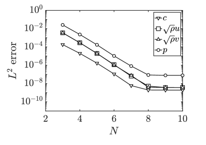
(a) $\Delta t=10^{-4}$

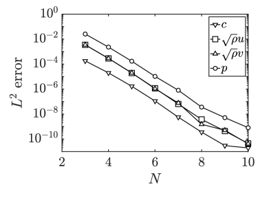
(b) $\Delta t=10^{-5}$

Figure 1: Exponential convergence of the manufactured solution (151) as the polynomial order increases. We represent the L² errors in concentration, $x$– and $y$–momentum, and pressure. The polynomial order ranges from 3 to 10, and we integrate in time until $t_{F}=0.1$ with two time step sizes: $\Delta t=10^{-4}$ and $10^{-5}$. All physical parameters are given in Table 1

Figs. 1(a) and 1(b) show typical and expected error behavior: an approximately linear semi-log convergence for lower polynomial orders implying exponential convergence of the error (i.e. under–resolved solution in space), and error stagnation for higher orders (under–resolved solution in time). The stagnation error threshold can be controlled with $\Delta t$, as shown in Fig. 1(b).

For the next test configuration, we use polynomial orders $N=2,3,4$ and $5$, and meshes with $4^{2},6^{2},8^{2},12^{2}$ and $16^{2}$ elements for an $h-$type convergence study. The time–step is $\Delta t=5\cdot 10^{-5}$. We solve the manufactured solution problem (151), and summarize the errors in Table 2. An estimate of the scheme’s order of convergence is provided there. We note that for the momentum components, the convergence orders are as expected, as they are close to $N+1$. For the pressure, the order of convergence is somewhat smaller (closer to $N$), which was also experienced in 2017:Bassi ; 2019:Manzanero-iNS . The convergence is also not optimal for the concentration; for even polynomials, the convergence can surpass the theoretical $N+1$ value, while for odd polynomials, the convergence rate is roughly $N$ in most of the cases. This effect was also noticed in 2019:Manzanero-CH , whose nature remains unclear.

Table 2: Manufactured solution (151) convergence analysis: we use $4^{3}$, $8^{3}$, and $16^{3}$ meshes, and $N=2,3,4$ and 5. The final time is $t_{F}=0.1$, and we use the IMEX BDF2 scheme with $\Delta t=5\cdot 10^{-5}$

	Mesh	$c$ error	order	$\sqrt{\rho}u$ error	order	$\sqrt{\rho}v$ error	order	$p$ error	order
N=2	$4^{2}$	1.35E-03	–	3.39E-02	–	3.39E-02	–	2.22E-01	–
	$6^{2}$	8.27E-04	1.21	1.24E-02	2.47	1.24E-02	2.47	9.02E-02	2.22
	$8^{2}$	4.40E-04	2.19	5.96E-03	2.56	5.95E-03	2.56	4.68E-02	2.28
	$12^{2}$	1.30E-04	3.01	2.04E-03	2.65	2.03E-03	2.65	1.78E-02	2.39
	$16^{2}$	5.35E-05	3.08	9.23E-04	2.75	9.23E-04	2.75	8.67E-03	2.50
N=3	$4^{2}$	1.81E-04	–	3.49E-03	–	3.50E-03	–	2.57E-02	–
	$6^{2}$	5.71E-05	2.85	8.28E-04	3.55	8.29E-04	3.55	6.81E-03	3.27
	$8^{2}$	2.76E-05	2.53	2.90E-04	3.65	2.91E-04	3.65	2.57E-03	3.39
	$12^{2}$	9.53E-06	2.62	6.34E-05	3.75	6.37E-05	3.74	6.17E-04	3.52
	$16^{2}$	4.36E-06	2.72	2.10E-05	3.83	2.12E-05	3.83	2.17E-04	3.64
N=4	$4^{2}$	1.99E-05	–	2.89E-04	–	2.87E-04	–	2.31E-03	–
	$6^{2}$	5.27E-06	3.28	4.40E-05	4.64	4.40E-05	4.62	3.94E-04	4.36
	$8^{2}$	7.50E-07	6.78	1.12E-05	4.75	1.12E-05	4.75	1.09E-04	4.47
	$12^{2}$	8.46E-08	5.38	1.55E-06	4.89	1.55E-06	4.89	1.70E-05	4.59
	$16^{2}$	1.94E-08	5.12	3.61E-07	5.05	3.61E-07	5.05	4.42E-06	4.68
N=5	$4^{2}$	1.69E-06	–	1.94E-05	–	1.98E-05	–	1.71E-04	–
	$6^{2}$	1.91E-07	5.38	1.96E-06	5.65	1.97E-06	5.70	1.87E-05	5.46
	$8^{2}$	4.67E-08	4.89	3.76E-07	5.74	3.77E-07	5.74	3.78E-06	5.57
	$12^{2}$	6.43E-09	4.89	3.64E-08	5.76	3.65E-08	5.76	3.79E-07	5.67
	$16^{2}$	1.63E-09	4.77	7.08E-09	5.69	7.11E-09	5.69	7.47E-08	5.64

5.2 Assessing robustness: random initial condition

We also assess the robustness of the scheme by introducing a random initial condition. Because the scheme developed here is entropy stable even for severely under–resolved solutions, the numerical implementation should not crash, as long as the time–step is small enough to stay within the time integrator stability region and the positivity condition is satisfied.

As a point of reference, and only in this section, we also consider the DG scheme using Gauss points. The standard DG method with Gauss points does not satisfy the SAT property 2009:Kopriva and the proofs developed for semi–discrete stability do not carry over. As a result, the standard scheme is not provably stable. To make the comparison even more stark, we compare robustness of the Gauss scheme with upwind flux dissipation to the new Gauss–Lobatto method with only central fluxes.

We solve the problem on the domain $\Omega=[0,1]^{3}$, and on a three–dimensional $4^{3}$ element Cartesian mesh. We initialize the solution using uniform random numbers in $[0,1]$ for concentration, and in $[-1,1]$ for velocities and pressure. We use a high density ratio ($\rho_{1}/\rho_{2}=1000$), and Reynolds number $Re=10^{6}$ so that physical viscosity will have only a weak stabilizing effect. The rest of the parameters are given in Table 3.

Table 3: Physical parameters for the random initial condition test problem

$\rho_{1}$	$\rho_{2}$ ($\text{kg}/\text{m}^{3}$)	$\eta_{1}$	$\eta_{2}$ (Pa$\cdot$s)	$\varepsilon$ (m)	$t_{CH}$ (s)	$c_{0}^{2}$ (m/s2)2	$\sigma$ (N/m)
1000.0	1.0	$10^{-3}$	$10^{-4}$	$0.75$	10.0	1.0E2	1.0

With Gauss–Lobatto points, the discrete entropy balance (149) shows that the free–energy time derivative $\mathcal{E}_{t}$ should be always negative as a result of viscous and chemical potential dissipation, for either central fluxes or the ERS. Moreover, the entropy remainder, defined as

$$\mathcal{R}\left(\mathcal{E}\right)=\frac{\mathop{}\!\mathrm{d}}{\mathop{}\!\mathrm{d}t}\left(\sum_{e}\left\langle\mathcal{J}\mathcal{E},1\right\rangle_{E,N}+\sum_{{\mathrm{boundary}\atop\mathrm{faces}}}\int_{f,N}f_{w}(C)\mathop{}\!\mathrm{d}S\right)+\left\langle\mathcal{J}\left(M_{0}|\svec{G}_{\mu}|^{2}+2\eta\mathcal{S}:\mathcal{S}\right),1\right\rangle_{E,N}\leqslant 0,$$ (153)

should be zero at each time step for central fluxes, and negative for the ERS. None of the statements regarding $\mathcal{E}_{t}$ or $\mathcal{R}\left(\mathcal{E}\right)$ being negative are guaranteed to hold for Gauss points by theory.

The entropy time derivative evolution is presented in Fig. 2, and the entropy remainder (153) in Fig. 3.

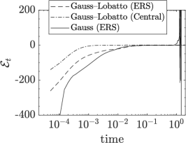
(a) $N=2$

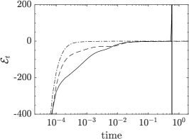
(b) $N=3$

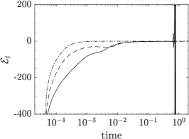
(c) $N=4$

Figure 2: Random chosen initial condition: evolution of the entropy time derivative $\mathcal{E}_{t}$ for three polynomial orders $N=2,3,4$. We consider three schemes: Gauss–Lobatto points with the ERS and central fluxes, and Gauss points with the ERS. For all the polynomial orders, using Gauss–Lobatto points is an entropy preserving scheme. The dissipation is a result of physical viscosity and chemical potential for central fluxes, to which the dissipation by the exact Riemann solver can added. On the contrary, the Gauss approximation entropy time derivative is not always negative, which numerically diverges as a result

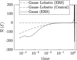
(a) $N=2$

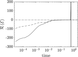
(b) $N=3$

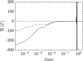
(c) $N=4$

Figure 3: Random initial condition: evolution of the entropy remainder (153) for three polynomial orders $N=2,3,4$. We consider three schemes: Gauss–Lobatto points with the ERS and central fluxes, and Gauss points with the ERS. The remainder studies the dissipation introduced by the scheme without considering physical viscosity and chemical potential. Thus, the Gauss–Lobatto scheme with the ERS is dissipative (always negative), the Gauss–Lobatto scheme with central fluxes is conserving (always zero), and the scheme with Gauss points is unstable and crashes

Both are presented for three polynomial orders ($N=2,3,4$), and for the three configurations described: Gauss–Lobatto points with ERS, Gauss–Lobatto points with central fluxes, and Gauss points with ERS. We find that the solutions follow the same pattern for the different polynomial orders. Gauss–Lobatto points are always stable, and the ERS enhances the stability (i.e. the entropy time derivative is always smaller or equal when compared to central fluxes). This is confirmed by looking at the entropy remainder in Fig. 3, which is machine precision for central fluxes, and negative for the ERS. Whereas for Gauss points, the solution is divergent (i.e. crashes) when $t\geq 1.53$. We see that for this case, Gauss points are more dissipative than Gauss–Lobatto points for the first steps, but then the opposite occurs when $t>10^{-2}$.

With a random initial condition, the Gauss approximation is prone to diverge, but might not. We ran another $100$ random initial conditions with different seeds until a final time $t_{F}=10.0$, of which 30/100 crashed. For the 70 simulations that did not crash, most of them experienced growth of their entropy at some points in time. We represent in Fig. 4 the number of simulations that crashed before the physical time on the horizontal axis.

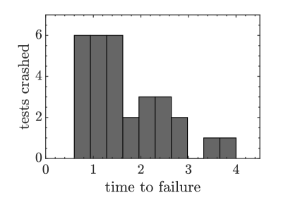
Figure 4: Random initial condition: we run 100 simulations modifying the random numbers sequence, of which 30 crashed with Gauss points. In this figure, the physical time in which the simulation diverged is represented. Although the other test passed the final time $t_{F}=10.0$, their entropy time derivative was found to be positive in several time–steps. None of the 100 simulations crashed with Gauss–Lobatto

Most often crashes occur early, i.e. times $t\approx 1.0$, after which the simulation is less likely to crash. None of the simulations crashed if they stayed stable for more than 4.0 seconds. In other words, if it can be computed beyond the initial stages, it is more likely to continue.

We repeated the experiment for the entropy stable Gauss–Lobatto variant, to confirm that none of them crashed. There may be advantages to use Gauss points, because of higher accuracy per degree of freedom 2011:Gassner ; 2016:Manzanero , and indeed the scheme presented herein allows us to use Gauss points in practice. However, as it is not entropy stable, it might crash under certain conditions, perhaps severely under–resolved simulations like high Reynolds turbulent flows, etc.

5.3 Static bubble

In this test problem we solve a steady two–dimensional bubble and validate the pressure jump that results from surface tension. In the domain $\Omega=[0,1]\times[0,1]$, the initial condition for the concentration is

$$c(x,y;0)=\frac{1-\tanh\left(-\frac{r-0.25}{\zeta}\right)}{2},~{}~{}r=\sqrt{(x-0.5)^{2}+(y-0.5)^{2}},~{}~{}\zeta=2.5\cdot 10^{-3},$$ (154)

which approximates a circle with radius $R_{0}=0.25$. Since we project the initial condition into our polynomial ansatz, the radius obtained, $R_{e}$, subtly differs to $R_{0}$. The analytical pressure jump between outside and inside of the bubble $\Delta p_{a}$ is given by the Poisson law,

$$\Delta p_{a}=p_{i}-p_{e}=p(0.5,0.5)-p(1.0,0.5)=\frac{\sigma}{R_{e}}.$$ (155)

Note that we used the radius $R_{e}$, which is estimated from the final solution contour $c(x,y)=0.5$, to compute the analytical solution. The rest of the parameters, including the surface tension $\sigma=1$ N/m, are given in Table 4.

Table 4: Parameters of the Static bubble test problem

Grid	$\rho_{1,2}$ ($\text{kg}/\text{m}^{3}$)	$\eta_{1,2}$ (Pa$\cdot$s)	$\varepsilon$ (m)	$t_{CH}$ (s)	$c_{0}^{2}$ (m/s2)2	$\sigma$ (N/m)	$\Delta t$ (s)
$16^{2}$	1.0	1.0	$0.16$	7.0	1.0E3	1.0	$10^{-5}$
$32^{2}$	1.0	1.0	$0.08$	7.0	1.0E3	1.0	$5\cdot 10^{-6}$
$64^{2}$	1.0	1.0	$0.05$	7.0	1.0E3	1.0	$2.5\cdot 10^{-6}$

We apply periodic boundary conditions at the four physical boundaries, and use the first order IMEX scheme ($J=1$) until the residuals are kept lower than $10^{-7}$.

The results are summarized in Table 5, which are computed with polynomial order $N=2$ and three meshes $16^{2}$, $32^{2}$, and $64^{2}$. For all meshes, we compute the solution radius $R_{e}$, the analytical pressure jump $\Delta p_{a}$, which are compared to the numerical solution interior pressure, $p_{i}$, exterior pressure $p_{e}$, and pressure jump $\Delta p$. Here we refer to the static pressure, and not the auxiliary pressure (16). The results show that the pressure jump converges to that given by the Poisson law (155) as we refine the grid.

In the last column of Table 5 we represent the norm of the velocity, which is of the size of the residuals. This implies that no parasitic currents are produced using this formulation, which are common in alternative Navier–Stokes/Cahn–Hilliard formulations 2009:Lee . Usually, the size of the parasitic currents is $10^{-3}$ for this problem, and since they do not disappear as the grid is refined, they can dominate in low speed simulations.

Table 5: Results of the Static bubble test problem

Grid	$R_{e}$ (m)	$\Delta p_{a}$	$p_{i}$	$p_{e}$	$\Delta p$ (Pa)	$|\Delta p-\Delta p_{a}|/\Delta p_{a}$	$\|\svec{v}\|$
$16^{2}$	0.220	4.546	0.033	-4.571	4.604	$1.27\cdot 10^{-2}$	$4.0\cdot 10^{-10}$
$32^{2}$	0.240	4.175	0.029	-4.120	4.150	$6.09\cdot 10^{-3}$	$2.4\cdot 10^{-8}$
$64^{2}$	0.244	4.100	0.173	-4.094	4.111	$2.75\cdot 10^{-3}$	$3.7\cdot 10^{-9}$

5.4 Rising bubble

The rising bubble problem has been widely used in the multiphase flow community to assess the space–time accuracy and robustness of the methods 2009:Hysing ; 2007:Ding ; 2017:Hosseini . The problem follows the trajectory of a bubble submerged in a heavier fluid as it rises. We consider the domain $\left(x,y\right)\in[0,1]\times[0,2]$, and a circular bubble with center in $(0.5,0.5)$ and diameter $0.5$. The bubble is approximated with the initial condition,

$$c(x,y;0)=1-\frac{1}{2}\left(\tanh\left(-\frac{2\left(r-0.25\right)}{\varepsilon}\right)+1\right),~{}~{}r=\sqrt{(x-0.5)^{2}+(y-0.5)^{2}},$$ (156)

and the rest of the variables are initialized to zero. We consider a Cartesian mesh with element size $h=2^{-4}$, and a polynomial order $N=10$. The physical parameters are taken from 2009:Hysing and are summarized in Table 6.

Table 6: Physical parameters of the Rising bubble test problem

Test	$\rho_{1}$	$\rho_{2}$ ($\text{kg}/\text{m}^{3}$)	$\eta_{1}$	$\eta_{2}$ (Pa$\cdot$s)	$\varepsilon$ (m)	$t_{CH}$ (s)	$c_{0}^{2}$ (m/s2)2	$\sigma$ (N/m)	$g$ (m/s2)
1	1000.0	100.0	10.0	1.0	$0.03$	1.0E3	1.0E3	24.5	0.98
2	1000.0	1.0	10.0	0.1	$0.04$	1.0E4	1.0E3	1.96	0.98

We consider two tests: the first with moderate density ratio $\rho_{1}/\rho_{2}=10$, the second with large density ratio $\rho_{1}/\rho_{2}=1000$. The boundary conditions are free–slip walls in $x=0$ and $x=1$, and no–slip walls in $y=0$ and $y=2$. For the Test 1, the chemical characteristic time is not big enough to use the explicit Runge–Kutta, and we use the second order IMEX BDF method, with time–step $\Delta t=7.2\cdot 10^{-6}$. For the Test 2, we use the explicit third order Runge–Kutta, with $\Delta t=7.2\cdot 10^{-7}$. Although we use fixed time–stepping, in both cases the CFL number ($\mathrm{CFL}=16(N+1)\left(|u|+a\right)\Delta t$) is maintained close to 0.2.

Although the model presented in this paper is diffuse interface, we compare it to a sharp interface model. Moreover, in this test case we compare the artificial compressibility method to a pressure–correction method that enforces the incompressible constraint in a transient simulation. Thus, we can assess the validity of the model and its implementation.

The shape of the bubble at the final time $t=3.0$ is represented in Fig. 5. First, in Fig. 5(a), we represent the final shape of the interface by drawing three contour lines: $c=0.1$ in dash–dot, $c=0.5$ as a solid line, and $c=0.9$ as a dashed line. The sharp interface reference solution is represented with black dots. We find a good agreement in both the position and the shape of the bubble, as the $c=0.5$ contour follows the shape of the bubble, and the dots are always found inside the $c=0.1$ and $c=0.9$ contours. Next, in Fig. 5(b) we represent the concentration contour, with the velocity vectors on top. The solution obtained is also in agreement with other diffuse interface works 2017:Hosseini .

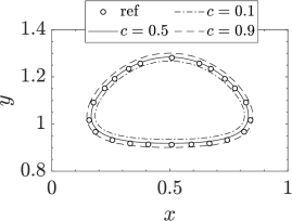
(a) Final shape of the bubble. We represent the interface with three contours: $c=0.1$, $c=0.5$, and $c=1.0$. The dots represent the sharp interface reference 2009:Hysing

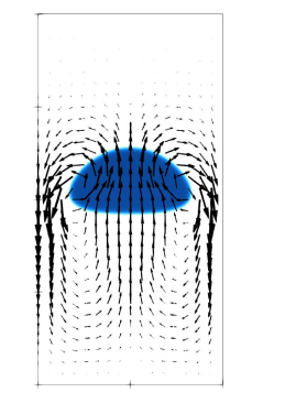
(b) Concentration contour at the final time $t=3$. The velocity field is also represented, showing the currents that raise the bubble

Figure 5: Rising bubble Test 1: position of the bubble and flow configuration at the final time $t=3.0$

In Fig. 6 we represent the evolution of the center of gravity (Fig. 6(a)) and the bubble rise velocity (Fig. 6(b)),

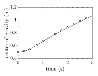
(a) Center of gravity

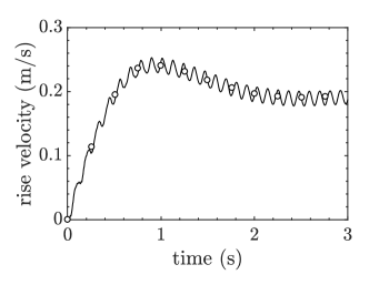
(b) Rise velocity

Figure 6: Rising bubble Test 1: evolution of the bubble center of gravity and rise velocity

$$X_{c}=\frac{1}{A}\sum_{e}\left\langle\mathcal{J}(1-C),X\right\rangle_{E,N},~{}~{}V_{c}=\frac{1}{A}\sum_{e}\left\langle\mathcal{J}(1-C),U\right\rangle_{E,N},~{}~{}A=\sum_{e}\left\langle\mathcal{J}(1-C),1\right\rangle_{E,N}.$$ (157)

Both center of gravity position and rise velocity show good agreement with the sharp interface reference. As for the rise velocity in Fig. 6(b), the oscillations are a result of the artificial compressibility pressure waves. One can reduce the amplitude of these oscillations by increasing the artificial sound speed $c_{0}$, but we have only found small differences in the evolution when increasing this parameter above the value used here.

Next, we solve the more challenging rising bubble Test 2 (see Table 6) with a higher density ($\rho_{1}/\rho_{2}=1000$) and viscosity ($\mu_{1}/\mu_{2}=100$) ratios. The evolution of the bubble and the flow configuration are represented in Fig. 7 at each $0.5$ second.

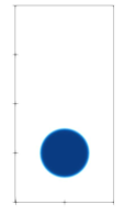
(a) $t=0$ s

(b) $t=0.5$ s

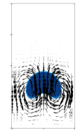
(c) $t=1.0$ s

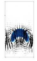
(d) $t=1.5$ s

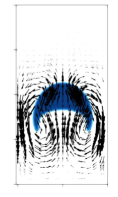
(e) $t=2.0$ s

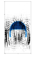
(f) $t=2.5$ s

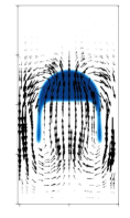
(g) $t=3.0$ s

Figure 7: Rising bubble Test 2: different snapshots showing the position of the bubble and the flow configuration

Both the shape and position of the bubble are in agreement with the sharp interface method 2009:Hysing , and other diffuse interface Cahn–Hilliard solvers 2017:Hosseini . Contrary to the rising bubble Test 1, the bubble now leaves behind an elongated skirt, which influences the velocity field. For completeness, we represent the center of gravity position and rise velocity as a function of time in Fig. 8, compared to the sharp interface solution provided in 2009:Hysing .

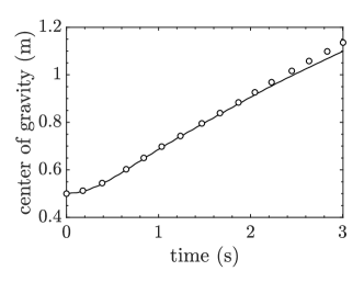
(a) Center of gravity

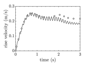
(b) Rise velocity

Figure 8: Rising bubble Test 2: evolution of the bubble center of gravity and rise velocity

Compared to the sharp interface reference, there are visible differences. However, it has been noted in 2009:Hysing ; 2017:Hosseini that the solution with different sets of equations might differ for this more challenging test case. Nonetheless, the evolution of the center of gravity and the rise velocity presented here agree with other diffuse interface solvers 2017:Hosseini .

5.5 Three–dimensional annular flow simulation

The last numerical experiment we present is a three–dimensional flow in a straight pipe ($L=10$) with circular section ($D=1$). Depending on the flow rates of fluid 1 and 2, the flow regime can be of different nature: stratified, slug, dispersed bubble, and annular. The last is the one we compute here, where one of the fluids behaves as a coating around the pipe surface. More details of the flow can be found in 1976:Taitel ; 2019:Manzanero-xPipe .

We construct a $z$–oriented mesh of the pipe with 8200 elements, and use a polynomial order $N=3$ (for both solutions and physical boundary representation). Note that this is the first time in this work that we use an unstructured curvilinear mesh. The cross section of the mesh is represented in Fig. 10(c). The physical parameters are taken from the literature 1976:Taitel and given in Table 7.

Table 7: Physical parameters of the annular flow

$\rho_{1}$	$\rho_{2}$ ($\text{kg}/\text{m}^{3}$)	$\eta_{1}$	$\eta_{2}$ (Pa$\cdot$s)	$\varepsilon$ (m)	$t_{CH}$ (s)	$c_{0}^{2}$ (m/s2)2	$\sigma$ (N/m)	$g$ (m/s2)	$\theta_{w}$ (deg)
1.0	5.0	$5\cdot 10^{-3}$	$10^{-2}$	$0.0424$	900.0	1.0E3	$2.5\cdot 10^{-4}$	1.0	45o

For the inflow and outflow boundary conditions, we construct auxiliary ghost states,

$$\mathbf{Q}^{in}=\left(\begin{array}[]{c}c_{in}\\ \sqrt{\rho\left(c_{in}\right)}\svec{u}_{in}\\ p\end{array}\right),~{}~{}\mathbf{Q}^{out}=\left(\begin{array}[]{c}c\\ \sqrt{\rho}\svec{u}\\ 0\end{array}\right),$$ (158)

with

$$\begin{split}c_{in}&=\frac{1}{2}+\frac{1}{2}\tanh\left(\frac{x-x_{0}}{\varepsilon}+\frac{1}{10}\sin\left(10z\right)+\frac{1}{10}\sin\left(20y\right)\right),\\ u_{in}&=0,\\ v_{in}&=0,\\ w_{in}&=\left(V_{1}c_{in}+V_{2}\left(1-c_{in}\right)\right)\left(1-4\frac{x^{2}+y^{2}}{D^{2}}\right),\\ p_{in}&=0.\end{split}$$ (159)

Furthermore, we use $\mathbf{Q}^{in}$ as the initial condition. The velocities $V_{1}$ and $V_{2}$, and interface position $x_{0}$ are set so that the superficial velocities, defined as,

$$V_{s1}=\frac{1}{\pi R^{2}}\int_{\mathrm{inlet}}V_{1}c_{in}\left(1-4\frac{x^{2}+y^{2}}{D^{2}}\right)\mathop{}\!\mathrm{d}S,~{}~{}V_{s2}=\frac{1}{\pi R^{2}}\int_{\mathrm{inlet}}V_{2}(1-c_{in})\left(1-4\frac{x^{2}+y^{2}}{D^{2}}\right)\mathop{}\!\mathrm{d}S,$$ (160)

are those found in 1976:Taitel . Precisely, we chose the velocities $V_{s1}=4.9$ m/s and $V_{s2}=0.06$ m/s, which produce the annular flow regime. If we place the interface between both fluids at $x_{0}=-0.262$ m (which yields a slip velocity $V_{1}-V_{2}=10$ m/s), the inlet velocities are $V_{1}=11.06$ m/s and $V_{2}=1.06$ m/s. At the walls, we also impose a contact angle $\theta_{w}=45^{o}$. With this configuration, we can use the third order Runge–Kutta scheme as time integrator with $\Delta t=10^{-5}$. In this simulation, we take into account the effect of gravity, which points in the negative $x$–direction.

The annular flow configuration is reached through an unstable mode, which makes the transient problem under–resolved until this mode is non–linearly damped and the final annular flow configuration is found. For that reason, we use a non–zero penalty parameter, $\beta$, on the Cahn–Hilliard equation. Precisely, we use the definition (108) with $\kappa_{\beta}=1$. Otherwise, we have found the scheme to be stable, but the solution obtained is mostly noise (i.e. it is not accurate). The introduction of the penalty parameter enhances the accuracy when the flow is under–resolved 2017:Ferrer .

We represent snapshots of the initial stages of the flow in Fig. 9. The fluid 2 is represented ($c\leqslant 0.5$), and colored by the vertical velocity (along the $x$–axis, $u$). We see that in the initial steps there is an unstable mode that grows until it changes the flow configuration. The vertical velocity contour shows that when fluid 2 rises above the interface it is dragged and accelerated by the quicker fluid 1, and the contrary occurs when it is confined below the interface because of the wall. This produces a wavy pattern at $t=0.3$s, which eventually wraps the fluid to the wall and produces the annular flow. In the early stages, the flow is highly under–resolved.

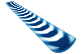
(a) $t=0.1$ s

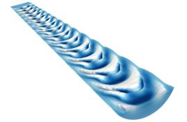
(b) $t=0.3$ s

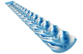
(c) $t=0.5$ s

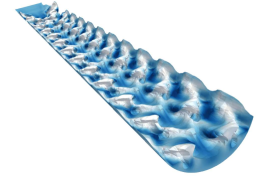
(d) $t=0.7$ s

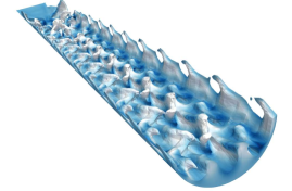
(e) $t=0.9$ s

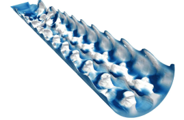
(f) $t=1.1$ s

Figure 9: Evolution of the physical mode that configures the annular flow. We have represented fluid 2 (i.e. $c\leqslant 0.5$), colored with vertical velocity, $u$. We see that during early times, there is an unstable physical mode that triggers the annular flow. When fluid 2 rises above the interface, it is dragged and accelerated by the quicker fluid 1. When it is confined below the interface, it is slowed down by the wall. This evolves non–linearly to the final state

We represent a final snapshot for $t=4.0$ s in Fig. 10, showing the contour $c\leqslant 0.5$ (i.e. the region occupied by fluid 2), colored by the longitudinal velocity (i.e. along the $z$–axis, $w$).

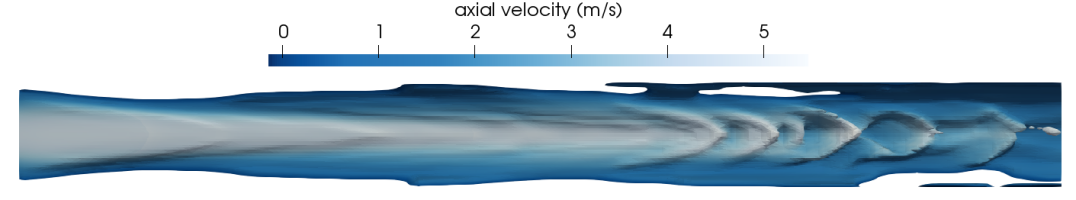
(a) Top view

(b) Side view

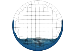
(c) Front view

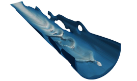
(d) Three dimensional view

Figure 10: Annular flow simulation. We present four view angles to the simulation at $t=4.0$ s. In the front view, the mesh cross section is also represented

Although the interface is flat at the inlet, the flow is unstable and breaks down into the annular flow configuration. The heavy fluid (fluid 2) is confined to the wall by the light fluid, which is introduced 82 times faster at the inlet. In Fig. 10(c) we represent the front view of the pipe, with the mesh detailed on top of it. We see that the flow gets smoother after the numerical and physical dissipation take over the mode breakdown after the under–resolved stages in Fig. 10.

6 Summary and conclusions

We have derived a two–phase flow model that combines the Cahn–Hilliard equation (3), a skew–symmetric version of the momentum equation (17), and an artificial compressibility method (18) to get the pressure. Among the many available options, the versions were chosen to satisfy an entropy inequality, (60). The entropy inequality bounds the mathematical entropy inside a finite domain $\Omega$ limited with wall boundary conditions by the entropy of the initial condition. As time marches, the mathematical entropy decreases as a result of the physical and the chemical potential dissipation.

We then constructed a DG approximation that satisfies the SBP–SAT property, which allowed us to mimic the continuous entropy analysis discretely. As is usual in a DG approximation, we had choices for the fluxes at inter–element and physical boundaries. We studied two options:

1. Entropy conserving, using central fluxes for the advective fluxes and the BR1 scheme for the diffusion. This choice gives a bound that discretely mimics the continuous entropy bound (60). This scheme is not of practical use, since some amount of numerical dissipation is required to provide accurate solutions when non–linear terms are present 2016:Gassner ; 2016:Manzanero ; 2017:Flad ; 2018:Manzanero-role . However, it serves as a baseline model to verify the stability proofs and to obtain a dissipation–free scheme.

2. Entropy stable, with an exact Riemann solver for the advective fluxes and the BR1 scheme for diffusive, with additional interface dissipation for the Cahn–Hilliard equation. This scheme transforms the entropy balance to an entropy inequality in the discrete version of (60), as a result of the numerical dissipation at the inter–element faces. This scheme uses the exact Riemann solver presented in 2017:Bassi for the incompressible Navier–Stokes equations, with an appropriate choice of the diamond fluxes that arise from the non–conservative terms, and a modification of the discrete entropy to account for solution discontinuities in the concentration as interfacial energy in the numerical solution.

Both the scheme and the stability proofs hold for three–dimensional unstructured meshes with hexahedral curvilinear elements.

We selected two choices to march the scheme in time: an explicit third–order Runge–Kutta method, and an implicit–explicit BDF with first or second order or accuracy. The former is used when the mobility is small enough to not severely restrict the time–step size, and the latter otherwise.

We test the scheme, addressing its accuracy with a manufactured solution convergence analysis, and its robustness by initializing the flow with random initial conditions. We showed that the scheme converges spectrally as expected, and that the scheme is robust in the sense that none of one hundred simulations crashed from random initial conditions, a high density ratio ($\rho_{2}/\rho_{1}=1000$), and a high Reynolds number ($\mathrm{Re}=10^{6}$). We compared the entropy–stable scheme with the more accurate Gauss counterpart (which is not provably entropy stable) to find that the latter crashes in $30\%$ of the simulations. We also solved commonly used static and rising bubble test problems to assess the steady state and transient accuracy of the solver. Finally we challenged the method by solving a three–dimensional pipe flow in the annular regime.

Appendix A Stability analysis of the alternative artificial compressibility model

We address the stability of the second artificial compressibility model (19). Since changes with respect to the original model (18) only affect to time–derivative terms, the analysis performed for spatial terms hold in this model, and we need only include the new time–derivative terms.

A.1 Continuous entropy analysis

The entropy analysis performed in Sec. 2.1 can be extended to the second artificial compressibility method (19). If we maintain the same entropy variables, all of the steps performed for space operators hold, and only the temporal terms contraction needs to be recomputed. Doing so,

$$\begin{split}&\mu c_{t}+\sqrt{\rho}\svec{u}\cdot\left(\sqrt{\rho}\svec{u}\right)_{t}-\frac{p\svec{\nabla}^{2}p_{t}}{\rho_{0}c_{0}^{2}}=\mathcal{F}_{t}+\mathcal{K}_{t}+\frac{\svec{\nabla}p\cdot\svec{\nabla}p_{t}}{\rho_{0}c_{0}^{2}}+\svec{\nabla}\cdot\left(\svec{f}_{t}^{\mathcal{E}}-\frac{p\svec{\nabla}p_{t}}{\rho_{0}c_{0}^{2}}\right)\\ &=\mathcal{F}_{t}+\mathcal{K}_{t}+\frac{|\svec{\nabla}p|_{t}^{2}}{2\rho_{0}c_{0}^{2}}+\svec{\nabla}\cdot\left(\svec{f}_{t}^{\mathcal{E}}-\frac{p\svec{\nabla}p_{t}}{\rho_{0}c_{0}^{2}}\right)=\mathcal{E}_{2,t}+\svec{\nabla}\cdot\svec{f}_{t}^{\mathcal{E}_{2}},\end{split}$$ (161)

with

$$\mathcal{E}_{2}=\mathcal{F}_{t}+\mathcal{K}_{t}+\frac{|\svec{\nabla}p|^{2}_{t}}{2\rho_{0}c_{0}^{2}},~{}~{}\svec{f}_{t}^{\mathcal{E}_{2}}=\frac{3}{2}\sigma\varepsilon c_{t}\svec{\nabla}c-\frac{p\svec{\nabla}p_{t}}{\rho_{0}c_{0}^{2}}.$$ (162)

The second artificial compressibility model is complemented with homogeneous Neumann boundary conditions for the pressure time derivative 1996:Shen ,

$$\svec{\nabla}p_{t}\cdot\svec{n}\biggr{|}_{\partial\Omega}=0,$$ (163)

which makes the pressure term in $\svec{f}_{t}^{\mathcal{E}_{2}}$ vanish at the boundaries. Hence, the entropy equation with physical boundary conditions for the second artificial compressibility method is identical to the original model (60)

$$\frac{\mathop{}\!\mathrm{d}}{\mathop{}\!\mathrm{d}t}\left(\bar{\mathcal{E}}_{2}+\int_{\partial\Omega}f_{w}(c)\mathop{}\!\mathrm{d}S\right)=-\int_{\Omega}\left(M_{0}|\svec{\nabla}\mu|^{2}+2\eta\mathsf{S}:\mathsf{S}\right)\mathop{}\!\mathrm{d}\svec{x}\leqslant 0,~{}~{}\bar{\mathcal{E}}_{2}=\int_{\Omega}\mathcal{E}_{2}\mathop{}\!\mathrm{d}\svec{x}.$$ (164)

A.2 Discretization

The discretization of the original artificial compressibility method (93) translates to the second method, where only the pressure time derivative terms need to be updated. We write the first order term using ${g}_{p}=\svec{\nabla}p$, transform the operators to local coordinates, integrate by parts, and replace the interface fluxes by a numerical flux and integrals by quadratures to get

$$\begin{split}\left\langle J\svec{\nabla}\cdot\svec{G}_{p,t},\varphi_{q}\right\rangle_{E}=\left\langle\svec{\nabla}_{\xi}\cdot\svec{\tilde{G}}_{p,t},\varphi_{q}\right\rangle_{E}\approx\int_{\partial e,N}\varphi_{q}\svec{G}_{p,t}^{\star}\cdot\svec{n}\mathop{}\!\mathrm{d}S-\left\langle\svec{\tilde{G}}_{p,t},\svec{\nabla}_{\xi}\varphi_{q}\right\rangle_{E,N}.\end{split}$$ (165)

For the interface fluxes, we use the BR1 method in interior faces,

$$P^{\star}=\{\!\{P\}\!\},~{}~{}\svec{G}_{p,t}^{\star}=\{\!\{\svec{G}_{p,t}\}\!\},$$ (166)

and a homogeneous Neumann boundary condition in physical boundaries,

$$P^{\star}=P,~{}~{}\svec{G}_{p,t}^{\star}\cdot\svec{n}=0.$$ (167)

A.3 Semi–discrete stability

As in the continuous analysis, we maintain the results from the original model, but update the time derivative terms (123),

$$\left\langle\mathcal{J}C_{t},\mu\right\rangle_{E,N}+\left\langle\mathcal{J}\left(\sqrt{\rho}\svec{U}\right)_{t},\sqrt{\rho}\svec{U}\right\rangle_{E,N}-\frac{1}{\rho_{0}c_{0}^{2}}\int_{\partial e,N}P\svec{G}_{p,t}^{\star}\cdot\svec{n}\mathop{}\!\mathrm{d}S+\frac{1}{\rho_{0}c_{0}^{2}}\left\langle\svec{\tilde{G}}_{p,t},\svec{\nabla}_{\xi}P\right\rangle_{E,N}.$$ (168)

From the gradient definition (93b), with test function $\svec{\varphi}_{g}=\svec{G}_{p,t}$

$$\left\langle\mathcal{J}\svec{G}_{p},\svec{G}_{p,t}\right\rangle_{E,N}=\int_{\partial e,N}\left(P^{\star}-P\right)\left(\svec{G}_{p,t}\cdot\svec{n}\right)\mathop{}\!\mathrm{d}S+\left\langle\svec{\tilde{G}}_{p,t},\svec{\nabla}_{\xi}P\right\rangle_{E,N},$$ (169)

we get the time derivative terms,

$$\begin{split}&\left\langle\mathcal{J}\mathcal{F}_{t},1\right\rangle_{E,N}-\int_{\partial e,N}\frac{3}{2}\sigma\varepsilon\left(C_{t}\svec{{G}}_{c}^{\star}+C_{t}^{\star}\svec{G}_{c}-C_{t}\svec{G}_{c}\right)\cdot\svec{n}\mathop{}\!\mathrm{d}S+\left\langle\mathcal{J}\left(\frac{1}{2}\rho V_{tot}^{2}\right)_{t},1\right\rangle_{E,N}\\ &+\left\langle\mathcal{J}\left(\frac{1}{\rho_{0}c_{0}^{2}}\svec{G}_{p}\right),\svec{G}_{p,t}\right\rangle_{E,N}-\frac{1}{\rho_{0}c_{0}^{2}}\int_{\partial e,N}\left(P\svec{G}_{p,t}^{\star}+P^{\star}\svec{G}_{p,t}-P\svec{G}_{p,t}\right)\cdot\svec{n}\mathop{}\!\mathrm{d}S\\ =&\left\langle\mathcal{J}\mathcal{F}_{t},1\right\rangle_{E,N}-\int_{\partial e,N}\frac{3}{2}\sigma\varepsilon\left(C_{t}\svec{{G}}_{c}^{\star}+C_{t}^{\star}\svec{G}_{c}-C_{t}\svec{G}_{c}\right)\cdot\svec{n}\mathop{}\!\mathrm{d}S+\left\langle\mathcal{J}\mathcal{K}_{t},1\right\rangle_{E,N}\\ &+\left\langle\mathcal{J}\left(\frac{1}{2\rho_{0}c_{0}^{2}}|\svec{G}_{p}|_{t}^{2}\right),1\right\rangle_{E,N}-\frac{1}{\rho_{0}c_{0}^{2}}\int_{\partial e,N}\left(P\svec{G}_{p,t}^{\star}+P^{\star}\svec{G}_{p,t}-P\svec{G}_{p,t}\right)\cdot\svec{n}\mathop{}\!\mathrm{d}S\\ =&\left\langle\mathcal{J}\mathcal{E}_{2,t},1\right\rangle_{E,N}-\int_{\partial e,N}\frac{3}{2}\sigma\varepsilon\left(C_{t}\svec{{G}}_{c}^{\star}+C_{t}^{\star}\svec{G}_{c}-C_{t}\svec{G}_{c}\right)\cdot\svec{n}\mathop{}\!\mathrm{d}S\\ &-\frac{1}{\rho_{0}c_{0}^{2}}\int_{\partial e,N}\left(P\svec{G}_{p,t}^{\star}+P^{\star}\svec{G}_{p,t}-P\svec{G}_{p,t}\right)\cdot\svec{n}\mathop{}\!\mathrm{d}S.\end{split}$$ (170)

We have now obtained the time derivative of the alternative discrete entropy $\mathcal{E}_{2}$ (162). The first boundary integral belongs to the Cahn–Hilliard equation and was shown not to contribute at interior faces (Sec. 4.4.3) if $\beta=0$, and to modify the entropy if $\beta>0$. The surface free–energy is obtained in physical boundary faces (Sec. 4.4.5). The last integral was added by the discretization of the pressure time derivative Laplacian. The contribution from interior edges with the BR1 scheme (166) is

$$\begin{split}\mathrm{IBT}_{\nabla^{2}p_{t}}=&\sum_{{\mathrm{interior}\atop\mathrm{faces}}}\int_{f,N}\left(\left\llbracket P\right\rrbracket\svec{G}_{p,t}^{\star}+\left\llbracket\svec{G}_{p,t}\right\rrbracket P^{\star}-\left\llbracket P\svec{G}_{p,t}\right\rrbracket\right)\cdot\svec{n}_{L}\mathrm{d}S\\ =&\sum_{{\mathrm{interior}\atop\mathrm{faces}}}\int_{f,N}\left(\left\llbracket P\right\rrbracket\{\!\{\svec{G}_{p,t}\}\!\}+\left\llbracket\svec{G}_{p,t}\right\rrbracket\{\!\{P\}\!\}-\left\llbracket P\svec{G}_{p,t}\right\rrbracket\right)\cdot\svec{n}_{L}\mathrm{d}S\\ =&0.\end{split}$$ (171)

For physical boundaries, we apply the homogeneous Neumann boundary condition (167), so that

$$\begin{split}\mathrm{PBT}_{\nabla^{2}p_{t}}=&\sum_{{\mathrm{boundary}\atop\mathrm{faces}}}\int_{f,N}\left(P\svec{G}_{p,t}^{\star}+P\svec{G}_{p,t}-P\svec{G}_{p,t}\right)\cdot\svec{n}\mathop{}\!\mathrm{d}S\\ =&\sum_{{\mathrm{boundary}\atop\mathrm{faces}}}\int_{f,N}\left(0+P\svec{G}_{p,t}\svec{n}-P\svec{G}_{p,t}\right)\cdot\svec{n}\mathop{}\!\mathrm{d}S\\ =&0.\end{split}$$ (172)

As a result, the alternative entropy (162) satisfies a continuous bound (164), and discrete entropy law,

$$\frac{\mathop{}\!\mathrm{d}}{\mathop{}\!\mathrm{d}t}\left(\bar{\mathcal{E}}_{2}^{\beta}+\sum_{{\mathrm{boundary}\atop\mathrm{faces}}}\int_{f,N}f_{w}(C)\mathop{}\!\mathrm{d}S\right)\leqslant-\sum_{e}\left\langle\mathcal{J}\left(M_{0}|\svec{G}_{\mu}|^{2}+2\eta\mathcal{S}:\mathcal{S}\right),1\right\rangle_{E,N}\leq 0,$$ (173)

where, similarly to (149), the inequality depends on whether the ERS and or central fluxes are used, and the choice of the interface penalty parameter $\beta$.

Appendix B Entropy contraction of the inviscid fluxes

We show the contraction of the inviscid fluxes (47) for the iNS/CH system. To do so, we replace the entropy variables, fluxes, and non–conservative terms,

$$\begin{split}\mathbf{w}^{T}\left(\svec{\nabla}\cdot\accentset{\,\leftrightarrow}{\mathbf{f}}_{e}\left(\mathbf{q}\right)+\sum_{m=1}^{5}\accentset{\,\leftrightarrow}{\boldsymbol{\phi}}_{m}\left(\mathbf{q}\right)\cdot\svec{\nabla}w_{m}\right)=&\mu\svec{\nabla}\cdot\left(c\svec{u}\right)+\frac{1}{2}u\svec{\nabla}\cdot\left(\rho u\svec{u}\right)+\frac{1}{2}v\svec{\nabla}\cdot\left(\rho v\svec{u}\right)+\frac{1}{2}w\svec{\nabla}\cdot\left(\rho w\svec{u}\right)+\svec{u}\cdot\svec{\nabla}p\\ &+\frac{1}{2}\rho u\svec{u}\cdot\svec{\nabla}u+\frac{1}{2}\rho v\svec{u}\cdot\svec{\nabla}v+\frac{1}{2}\rho w\svec{u}\cdot\svec{\nabla}w+c\svec{u}\cdot\svec{\nabla}\mu+p\svec{\nabla}\cdot\svec{u}\\ =&\svec{\nabla}\cdot\left(\left(\frac{1}{2}\rho v_{tot}^{2}+p+c\mu\right)\svec{u}\right)=\svec{\nabla}\cdot\svec{f}^{\mathcal{E}}_{e}.\end{split}$$ (174)

Thus, we see that the term $\svec{\nabla}\cdot\left(c\svec{u}\right)$ in the Cahn–Hilliard equation cancels the capillary pressure $c\svec{\nabla}\mu$ from the momentum non–conservative terms when multiplied by their respective entropy variables. Similarly, it reveals that momentum terms from the conservative and non–conservative parts cancel each other, and that the pressure term in the momentum equation cancels the velocity divergence term by way of the artificial compressibility equation.

Appendix C Point–wise discretization

In this section we list the steps to compute the solution time derivative with the DG approximation, (93). To get the point–wise values, we replace the test function by the Lagrange polynomials $l_{i}\left(\xi\right)l_{j}\left(\eta\right)l_{k}\left(\zeta\right)$. Details on the extraction of point–wise values can be found in 2009:Kopriva .

1. Compute the entropy variables, $\mathbf{W}$. The first entropy variable is the chemical potential, $\mu$, which is computed from (93d) and (93c),

   $$\begin{split}\mathcal{J}_{ijk}\svec{G}_{c,ijk}=&\left(C^{\star}-C\right)_{ijk}\left(\frac{\delta_{im}}{w_{i}}\mathcal{J}\svec{a}^{1}_{ijk}+\frac{\delta_{jm}}{w_{j}}\mathcal{J}\svec{a}^{2}_{ijk}+\frac{\delta_{km}}{w_{k}}\mathcal{J}\svec{a}^{3}_{ijk}\right)\biggr{|}^{m=N}_{m=0}\\ &+\mathcal{J}\svec{a}^{1}_{ijk}\sum_{m=0}^{N}D_{im}C_{mjk}+\mathcal{J}\svec{a}^{2}_{ijk}\sum_{m=0}^{N}D_{jm}C_{imk}+\mathcal{J}\svec{a}^{3}_{ijk}\sum_{m=0}^{N}D_{km}C_{ijm}\\ \mathcal{J}_{ijk}\mu_{ijk}=&\mathcal{J}_{ijk}F_{0}^{\prime}(C_{ijk})-\frac{3}{2}\sigma\varepsilon\left(\frac{\delta_{im}}{w_{i}}{\tilde{G}}_{c,ijk}^{1,\star}+\frac{\delta_{jm}}{w_{j}}{\tilde{G}}_{c,ijk}^{2,\star}+\frac{\delta_{km}}{w_{k}}{\tilde{G}}_{c,ijk}^{3,\star}\right)\biggr{|}_{m=0}^{m=N}\\ &+\frac{3}{2}\sigma\varepsilon\sum_{m=0}^{N}\left(\frac{w_{m}}{w_{i}}D_{mi}{\tilde{G}}_{c,mjk}^{1}+\frac{w_{m}}{w_{j}}D_{mj}{\tilde{G}}_{c,imk}^{2}+\frac{w_{m}}{w_{k}}D_{mk}{\tilde{G}}_{c,ijm}^{3}\right),\end{split}$$ (175)

   where $D_{ij}=l^{\prime}_{j}(\xi_{i})$ is the derivative matrix, and recall the definition of contravariant components (69). We then get the entropy variables from the current values of the state vector, $\mathbf{Q}$, and the chemical potential, $\mu$ computed by (175),

   $$\mathbf{W}_{ijk}=\left(\mu,\frac{Q_{2}}{\sqrt{\rho}},\frac{Q_{3}}{\sqrt{\rho}},\frac{Q_{4}}{\sqrt{\rho}},\frac{Q_{5}}{\rho_{0}c_{0}^{2}}\right)_{ijk},~{}~{}\rho=\rho_{1}\hat{C}+\rho_{2}\left(1-\hat{C}\right),~{}~{}\hat{C}=\min\left(\max\left(C,0\right),1\right).$$ (176)

2. Compute the gradient of the entropy variables $\accentset{\,\leftrightarrow}{\mathbf{G}}$ from (93b),

   $$\begin{split}\mathcal{J}_{ijk}\accentset{\,\leftrightarrow}{\mathbf{G}}_{ijk}=&\left(\mathbf{W}^{\star,T}-\mathbf{W}^{T}\right)_{ijk}\left(\frac{\delta_{im}}{w_{i}}\mathcal{J}\svec{a}^{1}_{ijk}+\frac{\delta_{jm}}{w_{j}}\mathcal{J}\svec{a}^{2}_{ijk}+\frac{\delta_{km}}{w_{k}}\mathcal{J}\svec{a}^{3}_{ijk}\right)\biggr{|}^{m=N}_{m=0}\\ &+\mathcal{J}\svec{a}^{1}_{ijk}\sum_{m=0}^{N}D_{im}\mathbf{W}_{mjk}+\mathcal{J}\svec{a}^{2}_{ijk}\sum_{m=0}^{N}D_{jm}\mathbf{W}_{imk}+\mathcal{J}\svec{a}^{3}_{ijk}\sum_{m=0}^{N}D_{km}\mathbf{W}_{ijm}.\end{split}$$ (177)

3. Compute the state vector time derivative,

   $$\begin{split}\mathcal{J}_{ijk}\underline{\mathbf{M}}_{ijk}\frac{\mathop{}\!\mathrm{d}\mathbf{Q}_{ijk}}{\mathop{}\!\mathrm{d}t}&+\left(\accentset{\,\leftrightarrow}{\mathbf{F}}_{e}^{\star}-\accentset{\,\leftrightarrow}{\mathbf{F}}_{e}+\sum_{m=1}^{5}\left(\accentset{\,\leftrightarrow}{\boldsymbol{\Phi}}_{m}W_{m}\right)^{\diamondsuit}-\accentset{\,\leftrightarrow}{\boldsymbol{\Phi}}_{m}W_{m}\right)_{ijk}\cdot\left(\frac{\delta_{im}}{w_{i}}\mathcal{J}\svec{a}^{1}_{ijk}+\frac{\delta_{jm}}{w_{j}}\mathcal{J}\svec{a}^{2}_{ijk}+\frac{\delta_{km}}{w_{k}}\mathcal{J}\svec{a}^{3}_{ijk}\right)\biggr{|}^{m=N}_{m=0}\\ &+\sum_{m=0}^{N}\left(D_{im}\tilde{\mathbf{F}}_{e,mjk}^{1}+D_{jm}\tilde{\mathbf{F}}_{e,imk}^{2}+D_{km}\tilde{\mathbf{F}}_{e,ijm}^{3}\right)\\ &+\sum_{p=1}^{N}\sum_{m=1}^{5}\left(\tilde{\boldsymbol{\Phi}}_{m,ijk}^{1}D_{ip}W_{m,pjk}+\tilde{\boldsymbol{\Phi}}_{m,ijk}^{2}D_{jp}W_{m,ipk}+\tilde{\boldsymbol{\Phi}}_{m,ijk}^{3}D_{kp}W_{m,ijp}\right)\\ =&\left(\frac{\delta_{im}}{w_{i}}\tilde{\mathbf{F}}_{v,ijk}^{1,\star}+\frac{\delta_{jm}}{w_{j}}\tilde{\mathbf{F}}_{v,ijk}^{2,\star}+\frac{\delta_{km}}{w_{k}}\tilde{\mathbf{F}}_{v,ijk}^{3,\star}\right)\biggr{|}_{m=0}^{m=N}\\ &+\sum_{m=0}^{N}\left(\frac{w_{m}}{w_{i}}D_{mi}\tilde{\mathbf{F}}^{1}_{v,mjk}+\frac{w_{m}}{w_{j}}D_{mj}\tilde{\mathbf{F}}^{2}_{v,imk}+\frac{w_{m}}{w_{k}}D_{mk}\tilde{\mathbf{F}}^{3}_{v,ijm}\right)+\mathcal{J}_{ijk}\mathbf{S}_{ijk}.\end{split}$$ (178)

References

• (1) M. Sussman, K. M. Smith, M. Y. Hussaini, M. Ohta, R. Zhi-Wei, A sharp interface method for incompressible two-phase flows, Journal of computational physics 221 (2) (2007) 469–505.
• (2) E. Olsson, G. Kreiss, A conservative level set method for two phase flow, Journal of computational physics 210 (1) (2005) 225–246.
• (3) J. Lowengrub, L. Truskinovsky, Quasi–incompressible Cahn–Hilliard fluids and topological transitions, Proceedings of the Royal Society of London. Series A: Mathematical, Physical and Engineering Sciences 454 (1978) (1998) 2617–2654.
• (4) J. W. Cahn, J. E. Hilliard, Free energy of a nonuniform system. I. Interfacial free energy, The Journal of chemical physics 28 (2) (1958) 258–267.
• (5) J. W. Cahn, J. E. Hilliard, Free energy of a nonuniform system. III. Nucleation in a two-component incompressible fluid, The Journal of chemical physics 31 (3) (1959) 688–699.
• (6) J. Shen, On a new pseudocompressibility method for the incompressible Navier-Stokes equations, Applied numerical mathematics 21 (1) (1996) 71–90.
• (7) B. S. Hosseini, S. Turek, M. Möller, C. Palmes, Isogeometric analysis of the Navier–Stokes–Cahn–Hilliard equations with application to incompressible two-phase flows, Journal of Computational Physics 348 (2017) 171–194.
• (8) J. Manzanero, G. Rubio, D. A. Kopriva, E. Ferrer, E. Valero, A free-energy stable nodal discontinuous Galerkin approximation with summation-by-parts property for the Cahn-Hilliard equation, arXiv preprint arXiv:1902.08089.
• (9) J. Manzanero, G. Rubio, D. A. Kopriva, E. Ferrer, E. Valero, Entropy-stable discontinuous Galerkin approximation with summation-by-parts property for the incompressible Navier-Stokes equations with variable density and artificial compressibility, arXiv preprint arXiv:1907.05976.
• (10) T.C. Fisher and M.H. Carpenter, High-order entropy stable finite difference schemes for nonlinear conservation laws: Finite domains, Journal of Computational Physics 252 (2013) 518–557.
• (11) M. H. Carpenter, T. C. Fisher, E. J. Nielsen, S. H. Frankel, Entropy stable spectral collocation schemes for the Navier-Stokes equations: Discontinuous interfaces, SIAM Journal on Scientific Computing 36 (5) (2014) B835–B867.
• (12) J. Chan, D. C. Del Rey Fernández, M. H. Carpenter, Efficient entropy stable Gauss collocation methods, SIAM Journal on Scientific Computing 41 (5) (2019) A2938–A2966.
• (13) D.A. Kopriva and G.J. Gassner, An energy stable discontinuous Galerkin spectral element discretization for variable coefficient advection problems, SIAM Journal on Scientific Computing 36 (4) (2014) A2076–A2099.
• (14) J. Manzanero, G. Rubio, E. Ferrer, E. Valero and D.A. Kopriva, Insights on aliasing driven instabilities for advection equations with application to Gauss-Lobatto discontinuous Galerkin methods, Journal of Scientific Computing.
• (15) G.J. Gassner, A skew-symmetric discontinuous Galerkin spectral element discretization and its relation to SBP-SAT finite difference methods, SIAM Journal on Scientific Computing 35 (3) (2013) 1233–1256.
• (16) G.J. Gassner, A. Winters, Andrew, F. Hindenlang, D.A. Kopriva, The BR1 scheme is stable for the compressible Navier-Stokes equations, Journal of Scientific Computing.
• (17) G. J. Gassner, A. R. Winters, D. A. Kopriva, A well balanced and entropy conservative discontinuous Galerkin spectral element method for the shallow water equations, Applied Mathematics and Computation 272 (2016) 291–308.
• (18) G.J. Gassner, A.R. Winters and D.A. Kopriva, Split form nodal discontinuous Galerkin schemes with Summation-By-Parts property for the compressible Euler equations, Journal of Computational Physics, in Press.
• (19) A.R. Winters and G.J. Gassner, Affordable, entropy conserving and entropy stable flux functions for the ideal MHD equations, Journal of Computational Physics 304 (2016) 72 – 108.
• (20) P. C. Hohenberg, B. I. Halperin, Theory of dynamic critical phenomena, Reviews of Modern Physics 49 (3) (1977) 435.
• (21) J. Shen, X. Yang, Energy stable schemes for Cahn–Hilliard phase-field model of two-phase incompressible flows, Chinese Annals of Mathematics, Series B 31 (5) (2010) 743–758.
• (22) J.-L. Guermond, L. Quartapelle, A projection fem for variable density incompressible flows, Journal of Computational Physics 165 (1) (2000) 167–188.
• (23) H. Ding, P. D. Spelt, C. Shu, Diffuse interface model for incompressible two-phase flows with large density ratios, Journal of Computational Physics 226 (2) (2007) 2078–2095.
• (24) S. Dong, Multiphase flows of N immiscible incompressible fluids: A reduction-consistent and thermodynamically-consistent formulation and associated algorithm, Journal of Computational Physics 361 (2018) 1–49.
• (25) F. Bassi, F. Massa, L. Botti, A. Colombo, Artificial compressibility Godunov fluxes for variable density incompressible flows, Computers & Fluids 169 (2018) 186–200.
• (26) H. Abels, H. Garcke, G. Grün, Thermodynamically consistent, frame indifferent diffuse interface models for incompressible two-phase flows with different densities, Mathematical Models and Methods in Applied Sciences 22 (03) (2012) 1150013.
• (27) J. Shen, Pseudo-compressibility methods for the unsteady incompressible Navier-Stokes equations, in: Proceedings of the 1994 Beijing symposium on nonlinear evolution equations and infinite dynamical systems, 1997, pp. 68–78.
• (28) X. Feng, J. Kou, S. Sun, A novel energy stable numerical scheme for Navier-Stokes-Cahn-Hilliard two-phase flow model with variable densities and viscosities, in: International Conference on Computational Science, Springer, 2018, pp. 113–128.
• (29) G. Zhu, H. Chen, J. Yao, S. Sun, Efficient energy-stable schemes for the hydrodynamics coupled phase-field model, Applied Mathematical Modelling 70 (2019) 82–108.
• (30) J. Shen, X. Yang, Decoupled, energy stable schemes for phase-field models of two-phase incompressible flows, SIAM Journal on Numerical Analysis 53 (1) (2015) 279–296.
• (31) F. Boyer, C. Lapuerta, S. Minjeaud, B. Piar, M. Quintard, Cahn–Hilliard/Navier–Stokes model for the simulation of three-phase flows, Transport in Porous Media 82 (3) (2010) 463–483.
• (32) E. Tadmor, Entropy stability theory for difference approximations of nonlinear conservation laws and related time-dependent problems, Acta Numerica 12 (2003) 451–512.
• (33) S. Dong, On imposing dynamic contact-angle boundary conditions for wall-bounded liquid–gas flows, Computer Methods in Applied Mechanics and Engineering 247 (2012) 179–200.
• (34) D. A. Kopriva, Metric identities and the discontinuous spectral element method on curvilinear meshes, Journal of Scientific Computing 26 (3) (2006) 301.
• (35) D.A. Kopriva, Implementing spectral methods for partial differential equations, Springer Netherlands, 2009.
• (36) D. A. Kopriva, A polynomial spectral calculus for analysis of DG spectral element methods, in: Spectral and High Order Methods for Partial Differential Equations ICOSAHOM 2016, Springer, 2017, pp. 21–40.
• (37) M. Bohm, A. R. Winters, G. J. Gassner, D. Derigs, F. Hindenlang, J. Saur, An entropy stable nodal discontinuous Galerkin method for the resistive MHD equations. part I: Theory and numerical verification, Journal of Computational Physics.
• (38) F. Bassi and S. Rebay, A high-order accurate discontinuous finite element method for the numerical solution of the compressible Navier-Stokes equations, Journal of Computational Physics 131 (2) (1997) 267 – 279.
• (39) E. Toro, Riemann solvers and numerical methods for fluid dynamics, Springer, 2009.
• (40) J. Manzanero, A.M. Rueda–Ramírez, G. Rubio and E. Ferrer, The Bassi Rebay 1 scheme is a special case of the Symmetric Interior Penalty formulation for discontinuous Galerkin discretisations with Gauss–Lobatto points, Journal of Computational Physics 363 (2018) 1 – 10.
• (41) J.H. Williamson, Low-storage Runge–Kutta schemes, Journal of Computational Physics.
• (42) G.J. Gassner and D.A. Kopriva, A comparison of the dispersion and dissipation errors of Gauss and Gauss-Lobatto discontinuous Galerkin spectral element methods, SIAM Journal on Scientific Computing 33 (5) (2011) 2560–2579.
• (43) J. Manzanero, G. Rubio, E. Ferrer and E. Valero, Dispersion-dissipation analysis for advection problems with nonconstant coefficients: Applications to discontinuous Galerkin formulations, SIAM Journal on Scientific Computing 40 (2) (2018) A747–A768.
• (44) T. Lee, Effects of incompressibility on the elimination of parasitic currents in the lattice Boltzmann equation method for binary fluids, Computers & Mathematics with Applications 58 (5) (2009) 987–994.
• (45) S.-R. Hysing, S. Turek, D. Kuzmin, N. Parolini, E. Burman, S. Ganesan, L. Tobiska, Quantitative benchmark computations of two-dimensional bubble dynamics, International Journal for Numerical Methods in Fluids 60 (11) (2009) 1259–1288.
• (46) Y. Taitel, A. Dukler, A model for predicting flow regime transitions in horizontal and near horizontal gas-liquid flow, AIChE journal 22 (1) (1976) 47–55.
• (47) J. Manzanero, C. Redondo, E. Ferrer, E. Valero, A high–order discontinuous Galerkin solver for multiphase flows, In Lecture notes in computational science and engineering ICOSAHOM 2018. (Accepted for publication).
• (48) E. Ferrer, An interior penalty stabilised incompressible Discontinuous Galerkin - Fourier solver for implicit Large Eddy Simulations, Journal of Computational Physics 348 (2017) 754–775.
• (49) David Flad and Gregor Gassner, On the use of kinetic energy preserving DG-schemes for large eddy simulation, Journal of Computational Physics 350 (Supplement C) (2017) 782 – 795.
• (50) J. Manzanero, E. Ferrer, G. Rubio, E. Valero, On the role of numerical dissipation in stabilising under-resolved turbulent simulations using discontinuous Galerkin methods, arXiv preprint arXiv:1805.10519.