Multi-wavelength campaign on NGC 7469
V. Analysis of the HST/COS observations:
Super solar metallicity, distance, and trough variation models

Abstract

Context. AGN outflows are thought to influence the evolution of their host galaxies and their super massive black holes. To better understand these outflows, we executed a deep multiwavelength campaign on NGC 7469. The resulting data, combined with those of earlier epochs, allowed us to construct a comprehensive physical, spatial, and temporal picture for this AGN wind.

Aims. Our aim is to determine the distance of the UV outflow components from the central source, their abundances and total column-density, and the mechanism responsible for their observed absorption variability.

Methods. We studied the UV spectra acquired during the campaign as well as from three previous epochs (2002-2010). Our main analysis tools are ionic column-density extraction techniques and photoionization models (both equilibrium and time-dependent models) based on the code Cloudy.

Results. For component 1 (at –600 km s^-1) our findings include the following: metallicity that is roughly twice solar; a simple model based on a fixed total column-density absorber, reacting to changes in ionizing illumination that matches the different ionic column densities derived from four spectroscopic epochs spanning 13 years; and a distance of R=$6^{+2.5}_{-1.5}$ pc from the central source. Component 2 (at –1430 km s^-1) has shallow troughs and is at a much larger $R$. For component 3 (at –1880 km s^-1) our findings include: a similar metallicity to component 1; a photoionization-based model can explain the major features of its complicated absorption trough variability and an upper limit of 60 or 150 pc on $R$. This upper limit is consistent and complementary to the X-ray derived lower limit of 12 or 31 pc for $R$. The total column density of the UV phase is roughly 1% and 0.1% of the lower and upper ionization components of the warm absorber, respectively.

Conclusions. The NGC 7469 outflow shows super-solar metallicity similar to the outflow in Mrk 279, carbon and nitrogen are twice and four times more abundant than their solar values, respectively. Similar to the NGC 5548 case, a simple model can explain the physical characteristics and the variability observed in the outflow.

1 Introduction

Absorption outflows are detected as blueshifted troughs in the rest-frame spectrum of active galactic nuclei (AGN). Such outflows in powerful quasars can expel sufficient gas from their host galaxies to halt star formation, limit their growth, and lead to the co-evolution of the size of the host and the mass of its central super massive black hole (e.g., Ostriker et al. 2010; Hopkins & Elvis 2010; Soker & Meiron 2011; Ciotti et al. 2010; Faucher-Giguère et al. 2012; Borguet et al. 2013; Arav et al. 2013). Therefore, deciphering the properties of AGN outflows is crucial for testing their role in galaxy evolution.

Nearby bright Seyfert I objects are important laboratories for studying these outflows because they yield the following: high-resolution high-resolution UV data, which allow us to study the outflow kinematics, trough variability, and can yield diagnostics for their distance from the central source; and X-ray grating spectra that give the physical conditions for the bulk of the outflowing material (e.g., Steenbrugge et al. 2005; Gabel et al. 2005; Arav et al. 2007; Costantini et al. 2007; Kaastra et al. 2012, 2014; Arav et al. 2015). Therefore, such observations are a crucial stepping stone for quantifying outflows from the luminous (but distant) quasars, for which grating X-ray data are seldom available.

NGC 7469 exhibits three kinematically-distinct UV outflow absorption components with velocity centroids at $-540\leavevmode\nobreak\ {\rm km\leavevmode\nobreak\ s}^{-1}$, $-1430\leavevmode\nobreak\ {\rm km\leavevmode\nobreak\ s}^{-1}$, and $-1880\leavevmode\nobreak\ {\rm km\leavevmode\nobreak\ s}^{-1}$ for components 1, 2 and 3, respectively. The outflow in NGC 7469 has been previously studied by Kriss et al. (2003) and Scott et al. (2005), using UV data from FUSE and STIS as well as simultaneous X-ray observations from Chandra and XMM-Newton. The UV analysis from Kriss et al. (2003) examined a single epoch of FUSE spectra from 1999. Scott et al. (2005) obtained followup FUSE observations of NGC 7469 in 2002, in addition to STIS spectra in 2002 and again in 2004. These multi-epoch spectra revealed trough variability in all of the detected troughs in components 1 and 3 of the outflow.

To further explore the variability of the NGC 7469 outflow and establish its location and physical characteristics, we carried out a multiwavelength campaign in 2015 similar to our previous successful campaigns on Mrk 509 (Kaastra et al. 2011; Mehdipour et al. 2011; Kriss et al. 2011; Arav et al. 2012; Kaastra et al. 2012) and NGC 5548 (Kaastra et al. 2014; Arav et al. 2015). The 2015 campaign used XMM-Newton (Behar et al. 2017), NuSTAR (Middei et al. 2018), Chandra and Swift (Mehdipour et al. 2018), and the Hubble Space Telescope (HST) (this paper) to monitor NGC 7469 over a six-month interval. Our seven visits with XMM-Newton (Behar et al. 2017) revealed a photoionized X-ray wind at outflow velocities of –550, –950, and  –2050 km s^-1 that had not changed significantly in its properties since the prior XMM-Newton observations in 2000 (Blustin et al. 2003) and 2004 (Blustin et al. 2007), and the Chandra observation in 2002 (Scott et al. 2005). The new, deeper XMM-Newton spectra also revealed emission from photoionized gas at $-450\leavevmode\nobreak\ \rm km\leavevmode\nobreak\ s^{-1}$, which is compatible with being the same outflow producing the absorption. The lack of X-ray absorption-line variability on timescales of roughly a decade place the X-ray outflow at distances of $>$12–31 pc (Peretz et al. 2018). This is possibly compatible with the 1-kpc starburst ring surrounding the nucleus (Wilson et al. 1991), which is also detected in our X-ray observations (Mehdipour et al. 2018).

This paper analyzes the HST component of our campaign in detail, while using inferences from prior UV observations and all X-ray epochs. In Section 2 we describe the observations and define the epochs of spectral observation considered in the analysis. In Section 3 we describe the unabsorbed emission model and extract column density measurements from the absorption features. In Section 4 we model the photoionization structure of the outflow components and their variability. In section 5 we compare the physical parameter of the UV outflow with those inferred for the warm absorber. We summarize our findings, and compare them with other Seyfert outflows in Section 6.

2 Description of Observations

Previous to our 2015 campaign, NGC 7469 (J2000: RA=23 03 15.62, DEC=+08 52 26.4, z=0.016268) was observed twice by FUSE (1999 and 2002) and with the Hubble Space Telescope (HST) in three spectral epochs: 2002 (PID 9095), 2004 (PID 9802) and 2010 (PID 12212). Details of the UV spectral observations are given in Table 1.

The main component of our 2015 campaign to monitor the outflowing absorbing gas in NGC 7469 used seven observations with the Cosmic Origins Spectrograph (COS) on HST (PID 14054) to sample timescales ranging from 1 day to 6 months. Each of our seven observations were coordinated with simultaneous XMM-Newton observations as described in Behar et al. (2017). These COS spectra consist of two-orbit visits using gratings G130M and G160M to cover the 1130–1800 Å wavelength range at a nominal resolving power of $\sim$18,000 (Green et al. 2012). We also obtained two additional observations (PID 14242) using the blue-mode of grating G130M at a central wavelength setting of 1096 Å. These observations span wavelengths 930–1280 Å (with a gap from 1080–1100 Å) at a resolving power of $\sim$12,000 (Debes et al. 2016), and cover the O vi and Ly$\beta$ outflow troughs.

The first visit in 2015 occurred five months before the remaining visits, and we distinguish this visit as the 2015a epoch, whereas visits 2-9 were coadded and hereafter referred to as the 2015b epoch. The 2015b epoch spans $\Delta t=33.4$ days of observations which begin $\Delta t=164.8$ days after the 2015a epoch.

Table 1: Observation information for all epochs

Epoch	Obs Date	Instrument	Grating	Exp
1999	1999/12/06	FUSE	FUV	37.6ks
2002	2002/12/13	FUSE	FUV	7.0ks
	2002/12/13	HST:STIS	E140M	13.0ks
2004	2004/06/21	HST:STIS	E140M	22.8ks
2010	2010/10/16	HST:COS	G130M	2.1ks
			G160M	2.4ks
2015_v1a	2015/06/12	HST:COS	G130M	2.2ks
			G160M	2.4ks
2015_v2b	2015/11/24	HST:COS	G130M	2.2ks
			G160M	2.4ks
2015_v3b	2015/12/15	HST:COS	G130M	2.2ks
			G160M	2.4ks
2015_v4b	2015/12/22	HST:COS	G130Mc	12.9ks
2015_v5b	2015/12/23	HST:COS	G130M	2.2ks
			G160M	2.4ks
2015_v6b	2015/12/25	HST:COS	G130M	2.2ks
			G160M	2.4ks
2015_v7b	2015/12/26	HST:COS	G130M	2.2ks
			G160M	2.2ks
2015_v8b	2015/12/27	HST:COS	G130Mc	10.2ks
2015_v9b	2015/12/29	HST:COS	G130M	2.2ks
			G160M	2.4ks
aUsed as 2015a epoch. bCoadded as 2015b epoch.
cUsing the 1096 central wavelength setting.

Figure 1: HST/COS spectrum of NGC 7469 for the 2015b epoch covering the main outflow absorption features. We label the ionic absorption troughs for all 3 outflow components (C₁–C₃) from Ly$\alpha$, C iv and N v; NVb and NVr refer to the blue and red doublet components of the N v doublet, respectively, With similar meaning for CIVb and CIVr. Intervening absorption troughs are marked with black dashed lines. The continuum and BEL emission model is shown as a red solid line.

3 Spectral Analysis

Figure 1 shows data from the coadded 2015b epoch (see Table 1). The spectral regions in the plot cover the three absorption components as seen in Ly$\alpha$, N v and C iv. Components 3 and 1 have a substantial optical depth and exhibit significant variability in multiple ions between multiple epochs (see Figure 2). Therefore, we focus our study on those components. Component 2 has shallow troughs which make the analysis results more uncertain (see section 4.2). The absorption feature at the 1232 Å observed wavelength (see Figure 2) has a narrow profile and no metal-line absorption counterparts. In addition, the 1232 Å trough has the same depth in the 2 STIS epochs and the same depth (although shallower than the STIS depth) in the 3 COS epochs. We attribute the depth difference between the STIS and COS epochs to the different resolution and line-spread-function of the two instruments and not to real optical depth change. Therefore, we agree with Kriss et al. (2003) and Scott et al. (2005) who attributed the 1232 Å trough to intergalactic Ly$\alpha$ absorption.

Two of the outflow components (1 and 3) were previously seen in HST spectra of NGC 7469 by Kriss et al. (2003) and Scott et al. (2005). Component 2 was too weak to be noticeable in the lower S/N STIS spectra from 2002 and 2004. Component 2 is clearly visible in our new COS spectra (as well as in the archival 2010 spectrum), and it varies. We conclude that component 2 is part of the NGC 7469 outflow. Figure 2 shows the Ly$\alpha$ trough variability for all three components.

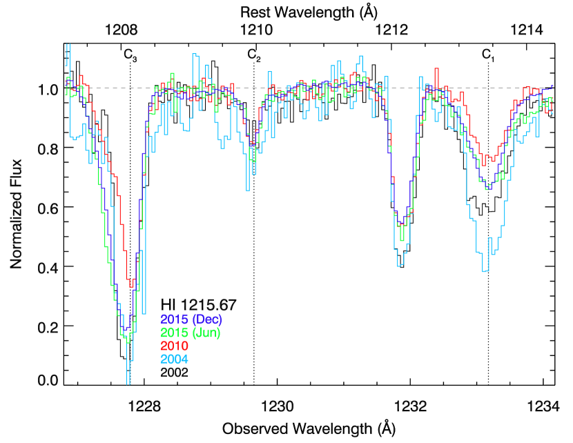
Figure 2: Normalized spectrum of the Ly$\alpha$ absorption for the three outflow components during the five major observation epochs. The trough at 1232 Å is a Ly$\alpha$ intervening absorber.

3.1 Emission Model

We model the emission separately for each epoch. The continuum is fit using a single power law, and the broad and narrow line emission features are fit ad-hoc with a superposition of one to four Gaussians per feature. The total emission model is shown in Figure 1. The emission in the spectral regions near the absorption troughs of component 3 is well-defined, but the lower velocity of component 1 locates its absorption troughs close to the corresponding peaks of the emission features. As such, the absorption depth of component 1 is affected by the emission model, and we assign to its measurements a larger uncertainty as a result.

3.2 Column Density Extraction

We extract the ionic column densities from each component for every epoch using the partial-covering (PC) method described in Arav et al. (2008) for the doublet transitions of C iv and N v. This method is performed assuming separate covering in each velocity bin. The remaining ions either have only one absorption trough (H i), are too shallow (Si iv), or too saturated (O vi) to use the PC method; so we measure the column densities using the apparent optical depth (AOD) method instead. We treat the AOD measurements of H i and O vi (when available) as lower limits. Si iv does not appear in the majority of epochs, so we determine upper limits to the column density in such cases by integrating the AOD of the blue doublet component over the velocity range of the trough.

The 2002 and 2015b epochs include spectral coverage of Ly$\beta$ absorption from component 3. However, the red wing of the absorption trough is contaminated by strong absorption from molecular hydrogen. We perform AOD integration on the blue half of the Ly$\beta$ trough, then double the value to obtain an estimation of the H i column density from Ly$\beta$. The derived ionic column densities ($N_{ion}$) are given in Table 2.

4 Photoionization Analysis

We used the spectral energy distribution (SED) continuum models for the 2002 and 2015 epochs as described by Mehdipour et al. (2018), see their figure 2. To determine the photoionization structure of the outflowing gas, we used the same method described in Arav et al. (2013): using the above SED to run a grid of photoionization models with the spectral synthesis code Cloudy (version c17.01 Ferland et al. 2017), by varying the total hydrogen column density ($N_{\mathrm{\scriptscriptstyle H}}$) and the hydrogen ionization parameter

$$U_{\mathrm{\scriptscriptstyle H}}\equiv\frac{Q_{\mathrm{\scriptscriptstyle H}}}{4\pi R^{2}n_{\mathrm{\scriptscriptstyle H}}c}$$ (1)

where $Q_{\mathrm{\scriptscriptstyle H}}$ is the rate of hydrogen-ionizing photons from the central source, $R$ is the distance to the outflow from the central source, $n_{\mathrm{\scriptscriptstyle H}}$ is the hydrogen number density ($n_{\mathrm{\scriptscriptstyle e}}\simeq 1.2n_{\mathrm{\scriptscriptstyle H}}$ in highly ionized plasma) and $c$ is the speed of light. We construct a phase plot depicting the solution by plotting the locus of models $(U_{\mathrm{\scriptscriptstyle H}},N_{\mathrm{\scriptscriptstyle H}})$ that correctly predict the observed $N_{\mathrm{ion}}$ measurements (within $1\sigma$ uncertainty) for each ion. These are shown in the top panel of Figure 3 as contours spanned by colored bands representing the uncertainties. We determine the best-fit model using chi-squared minimization.

Table 2: Column densities^a for the NGC 7469 outflow components

Ion		$v_{3}$			$v_{2}$			$v_{1}$
		$[-2070,-1800]^{b}$			$[-1470,-1370]^{b}$			$[-700,-410]^{b}$
Epoch 2002       relative UV flux 2.61c
H	i	$>$	14.22		$>$	13.07		$>$	13.87
N	v	$>$	14.85		$<$	13.14		$>$	13.97
Si	iv	$<$	12.69		$<$	12.16		$<$	12.85
C	iv	$>$	14.56		$>$	13.37			13.50	${}^{+0.15}_{-0.15}$
O	vi	$>$	14.98	$\,\!{}^{d}$	$<$	13.77		$>$	14.92
Epoch 2004       relative UV flux 1.0
H	i	$>$	14.25		$>$	13.31		$>$	14.01
N	v		14.67	${}^{+0.37}_{-0.37}$	$<$	12.62		$>$	14.11
Si	iv	$<$	12.57		$<$	12.78		$<$	13.33
C	iv	$>$	14.56		$>$	13.23			13.79	${}^{+0.1}_{-0.1}$
Epoch 2010       relative UV flux 5.15
H	i	$>$	13.89		$>$	12.97		$>$	13.47
N	v		14.73	${}^{+0.19}_{-0.19}$	$>$	13.09		$>$	13.62
Si	iv	$<$	12.72		$<$	12.26		$<$	12.37
C	iv	$>$	14.52		$>$	13.14		$<$	12.82
Epoch 2015a       relative UV flux 2.26
H	i	$>$	14.21		$>$	13.06		$>$	13.70
N	v		14.93	${}^{+0.65}_{-0.65}$	$<$	13.35		$>$	13.90
Si	iv	$<$	13.02		$<$	13.16		$<$	12.59
C	iv	$>$	14.89		$>$	12.99		$>$	13.26
Epoch 2015b       relative UV flux 1.94
H	i	$>$	14.12		$>$	13.01		$>$	13.65
N	v		14.95	${}^{+0.30}_{-0.30}$	$<$	13.39		$>$	13.84
Si	iv		12.95	${}^{+0.20}_{-0.20}$	$<$	12.86		$<$	12.39
C	iv	$>$	14.81		$>$	13.16		$>$	13.34
O	vi	$>$	15.08		$<$	13.98		$>$	14.88
$\,{}^{a}$Table values are log column densities ($\mathrm{cm}^{-2}$)
Lower limit are shown in blue, upper limits in red.
Measurements (and errors) are shown in black.
$\,{}^{b}$Integration limits in km $\mathrm{s}^{-1}$.
$\,{}^{c}$flux at 1170 Å relative to the 2004 flux
(2004 flux at 1170 Å = $1.20\times\rm 10^{-14}\leavevmode\nobreak\ erg\leavevmode\nobreak\ cm^{-2}\leavevmode\nobreak\ s^{-1}\leavevmode\nobreak\ \AA^{-1}$)
$\,{}^{d}$The O vi absorption trough only exists in Epoch 2002
and Epoch 2015b. See Section 2 for more details.

4.1 Component 1

Component 1 has a substantial optical depth and exhibits the strongest variability of all three components between multiple epochs (see Figure 2). We begin by constructing and discussing photoionization solutions, first for the 2015 data and then for all epochs. We then use time-dependent photoionization analysis to model the troughs variability, which leads to a distance determination for this component from the central source

4.1.1 Consistent photoionization solutions for all epochs

The portion of the SED responsible for the photoionization equilibrium of the species we observe with COS (H i, C iv, N v, O vi and Si iv) is between 13.6 eV to several hundred eV. Across this energy range, the ratio of the 2015 to the 2002 SED changed by a maximum of $\pm 15$% (see figure 2 in Mehdipour et al. 2018). Thus, we make the simple and restrictive assumption that the shape of the NGC 7469 Spectral SED is the same in all observed epochs from 2002–2015. Therefore, the changes in integrated flux and $U_{\mathrm{\scriptscriptstyle H}}$ are equal to changes in the measured UV flux (see Table 2). Since Ly$\alpha$ is a singlet, we methodically treat its individual AOD $N_{ion}$ measurements as lower limits (see Table 2). However, component 1 show trough variations that strongly correlate with the measured UV flux (see Figure 2 and Table 2). Quantitatively, from Table 2 we infer that for the largest flux variation, a factor of 5.2 ($\Delta\log(U_{\mathrm{\scriptscriptstyle H}})=0.7$) between 2004 and 2010, the AOD derived N(H i) changed by a factor of 3.5. With no saturation, and assuming photoionization equilibrium, the 2004 N(H i) should have been $\sim 7$ times higher than in 2010 (where we assumed $\log({U_{\mathrm{\scriptscriptstyle H}}}_{2004})=-1.3$ and $\log({U_{\mathrm{\scriptscriptstyle H}}}_{2010})=-0.6$, see below).

Assuming that a) the real change in N(H i) between the two epochs is indeed a factor of 7; and b) that the Ly$\alpha$ trough had the same covering factor in 2004 and 2010, we can perform a covering factor analysis on the two troughs (see section 3 of Arav et al. 2005, for the full formalism, including velocity dependence). The results are that the real N(H i) is only a few percent larger than the AOD value deduced from the shallower 2010 trough, but 100% larger than the AOD value deduced from the deeper 2004 trough. This result is consistent with the findings that when troughs from the same ionic species are saturated, the deeper trough is more saturated than the shallower one (Arav et al. 2018). We therefore use the 2010 N(H i) reported value as an actual measurement, and consider the deeper 2004 trough to be mildly saturated, where its N(H i) is two times the lower limit reported in Table 2.

Independent support for the mild-saturation scenario comes from the Ly$\beta$ observations in the 2002 and 2015b epochs. The center and entire blue wing of the Ly$\beta$ trough of component 1 ($-700<v<-500\leavevmode\nobreak\ {\rm km\leavevmode\nobreak\ s}^{-1}$) are heavily contaminated with galactic absorption. However, at roughly $-500{\rm km\leavevmode\nobreak\ s}^{-1}$ the galactic absorption disappears, and at that velocity, for component 1, an upper limit of $\tau$(Ly$\beta$)=0.05 is derived from the data for both epochs. At the same velocity (equivalent to 1233.4Å observed wavelength in figure 2), $\tau$(Ly$\alpha$)=0.32 and 0.25 for the 2002 and 2015b epochs, respectively. For a case of no saturation (i.e., an optically thin absorber) $\tau$(Ly$\alpha$)/$\tau$(Ly$\beta$)=6.2 (based on the ratio of the product of their oscillator-strength and wavelength). Therefore, the observed ratios between the measured $\tau$(Ly$\alpha$) and upper limit on $\tau$(Ly$\beta$) at $-500{\rm km\leavevmode\nobreak\ s}^{-1}$ (6.4 and 5, for the 2002 and 2015b epochs, respectively) are consistent with the expected value for an unsaturated absorber.

We note that the C iv and N v troughs respond similarly to changes in the UV flux, and therefore the nominal lower limits on their $N_{ion}$ are close to their actual values.

The top panel of figure 3 shows the photoioinization phase plot for the 2015b epoch, where we used the 2015 SED and assumed the proto-solar abundances given by Lodders et al. (2009). For C iv, N v and O vi, the $N_{ion}$ constraints are all lower limits, requiring the photoioinization solution to be inside or above their colored bands. Since we established that the N(H i) constraint is a measurement, the photoioinization solution has to be inside the red band. It is evident that there is no region on this plot that satisfies both the hydrogen and CNO constraints.

A physically plausible way to alleviate this issue is to invoke Super Solar Metallicity (SSM). As shown in dedicated studies, AGN outflows exhibit SSM. In the case of Mrk 279 (a Seyfert I with similar luminosity to NGC 7469) we found the following CNO abundances relative to solar (using the standard logarithmic notation) [C/H]=0.2–0.5, [O/H]=0–0.3 and [N/H]=0.4–0.7 (Arav et al. 2007). For the outflow observed in the Hubble-deep-field-south target QSO J2233–606, we found [C/H], [O/H] $\approx 0.5-0.9$ and [N/H] $\approx 1.1-1.3$ (Gabel et al. 2006). The SSM for the outflows in both objects is consistent with enhanced nitrogen production expected from secondary nucleosynthesis processes (Gabel et al. 2006), where [N/H]$\simeq$2[C/H]$\simeq$2[O/H]$\simeq$2[Si/H] (see model M5a of Hamann & Ferland 1993, which is used for obtaining abundances with different metallicities than proto-solar in Cloudy).

* *

Figure 3: Top: Photoionization phase plot showing the constraints for component 1 of epoch 2015b, where we use the 2015 NGC 7469 SED and proto-solar metallicity. Solid lines and associated colored bands represent the locus of $U_{\mathrm{\scriptscriptstyle H}}$, $N_{\mathrm{\scriptscriptstyle H}}$ models, which predict the measured $N_{\mathrm{ion}}$, and their $1\sigma$ uncertainties; dashed lines represent $N_{\mathrm{ion}}$ lower limits that permit a solution in the phase-space above them; and dotted lines represent $N_{\mathrm{ion}}$ upper limits that permit a solution in the phase-space below the line. Since the CNO lower limit bands do not intersect with the H i band, it is clear that there is no viable photoionization solution for this case. Middle: Same $N_{\mathrm{ion}}$ constraints and same SED as in the top panel, but assuming super-solar metallicity as described in section 4.1.1. The viable physical solution and its 1-$\sigma$ error are shown by the black dot and surrounding black oval, respectively. Bottom: Phase plot showing the photoionization constraints for component 1 in three different epochs, using the same SED and abundances used in the middle panel. Similar presentation to the other panels, where for clarity’s sake we do not show the errors on individual measurements, (the errors are similar to the ones shown in the middle panel). Most of the C iv, N v and Ly$\alpha$ constraints are lower limits. To help distinguish between them, we assign different length dashed lines for these lower limit constraints. The region between the three C iv constraints is shaded to help guide the eye. The ‘X’ symbols show the location of the derived photoionization solutions for the different epochs where $N_{\mathrm{\scriptscriptstyle H}}$ is kept constant and the difference in $U_{\mathrm{\scriptscriptstyle H}}$ is equal to the difference in the measured UV flux for each epoch.

In constructing a viable SSM photoionization model, we attempt to restrict the number of degrees of freedom (associated with SSM and otherwise) as much as possible. First, we assume that the chosen SSM must apply to all epochs. Second, we use metallicity enhancement that is both consistent with the Mrk 279 results and adheres to the enhanced nitrogen production expected from secondary nucleosynthesis processes described above. Thus, we use [C/H]=[O/H]=[Si/H]=0.35 and [N/H]=0.70, which yields a viable solution for the 2010 epoch constraints.

In the middle panel of figure 3 we show the photoioinization phase plot for the 2015b epoch, where we use the 2015 SED and assumed the SSM abundances values given above. The $N_{\mathrm{ion}}$ constraints are the same but their position on the $U_{\mathrm{\scriptscriptstyle H}}$–$N_{\mathrm{\scriptscriptstyle H}}$ plane is lower by roughly the inverse of their scaled abundances. This is because for an enheced abundance of a given element the $N_{\mathrm{\scriptscriptstyle H}}$ needed to satisfy its $N_{\mathrm{ion}}$ is smaller. The best fitting solution and its 1-$\sigma$ error are shown by the black dot and surrounding black oval, respectively.

Changing the abundances yields a solution for the 2015b epoch mainly due to the introduction of two new parameters (the coupled abundances for C, O and Si, and the abundance of N). It is the fits to the other epochs that makes this model physically robust. The models for the other epochs have no additional free parameters. Similar to our model for the NGC 5548 outflow (Arav et al. 2015), we require that: a) the $U_{\mathrm{\scriptscriptstyle H}}$ of the solution for each different epoch will differ by the ratio of the UV flux of the said epoch to the UV flux of the 2010 epoch (for which the abundances were determined to allow for a viable solution); and b) $N_{\mathrm{\scriptscriptstyle H}}$ is constant for all epochs. The last requirement follows our assertion below, that it is unlikely that significant amount of material will enter or exit the line of sight between 2002 and 2015 (see section 6).

The model for all 4 epochs is shown in the bottom panel of Figure 3. For clarity’s sake, we show constraints from only 3 epochs: those with the lowest and highest UV fluxes, 2004 and 2010, respectively, and 2015b, which has the highest S/N data and is the most recent. We also do not show the 1$\sigma$ error bars associated with the different constraints, but they are similar to the width of the colored ribbons on the top panel. Each of the solutions fit all the $N_{ion}$ constraints roughly within the error. We note that:
a) the Si iv constraint for all epochs is an upper limit which is trivially satisfied in all epochs as the solution needs to be below the upper limit curve.
b) we implicitly assume that the C iv and N v lower limits $N_{ion}$ reported in Table 2 are actual measurements as we ascribe their different values to our modeled photoionization changes.
Thus, this restrictive and simple model, which is based on a fixed total column-density absorber reacting to changes in ionizing illumination, matches the measured constraints spanning 13 years.

We note that even assuming the same SSM, the $U_{\mathrm{\scriptscriptstyle H}}$–$N_{\mathrm{\scriptscriptstyle H}}$ solution for the 2015b epoch in the bottom panel is slightly different than the one in the middle panel. That is because the middle panel solution was optimized to only the 2015b $N_{\mathrm{ion}}$. On the bottom panel all the solutions are fixed by the 2010 solution (see above) and therefore the $U_{\mathrm{\scriptscriptstyle H}}$–$N_{\mathrm{\scriptscriptstyle H}}$ solution for 2015b in the lower panel is not the same as in the middle panel. An important aspect of the 4 epochs solution is that the $U_{\mathrm{\scriptscriptstyle H}}$–$N_{\mathrm{\scriptscriptstyle H}}$ solution for 2015b in the bottom paneel is within the error ellipse of the pure 2015b solution.

Figure 4: Time-dependent photoionization solutions: starting from the photoionization equilibrium for the 2015b epoch (shown in the bottom panel of figure 3), we assume a step-function flux increase of 13% (see text), and track the changes in the relative fraction of N v for a range of $n_{\mathrm{\scriptscriptstyle e}}$. The log($n_{\mathrm{\scriptscriptstyle e}}$) of each solution labels each curve. The shortest time-scale where we measured definitive changes in the N v trough between two epochs was 700,000 seconds. In red we mark the N v fraction curve that shows a 50% change between the initial and final values after 700,000 seconds.

4.1.2 Distance determination from trough variability

Table 3: Time of 2015 Visits and Flux

Obs	Time	$f_{1170}$
	(MJD)a	($\rm 10^{-14}\leavevmode\nobreak\ erg\leavevmode\nobreak\ cm^{-2}\leavevmode\nobreak\ s^{-1}\leavevmode\nobreak\ \AA^{-1}$)
V01-2015	185.84	$2.71\pm 0.01$
V02-2015	350.62	$1.94\pm 0.01$
V03-2015	371.43	$2.32\pm 0.01$
V05-2015	379.38	$2.63\pm 0.01$
V06-2015	381.30	$2.46\pm 0.01$
V07-2015	382.95	$2.20\pm 0.01$
V09-2015	385.20	$2.44\pm 0.01$
aMJD-57,000

Component 1 exhibits variations in Ly$\alpha$, C iv and N v absorption strengths during the visits of the 2015 epochs. As detailed above, it is likely that these trough variations are the response of the absorber to changes in the ionizing flux. Tracking changes in column density of a given ion between different epochs along with flux monitoring can lead to estimates of $n_{\mathrm{\scriptscriptstyle e}}$. Then using equation (1), the distance $R$ can be determined (e.g., Gabel et al. 2005).

The timescale for photonionization changes is inversely proportional to $n_{e}$. Therefore, for a given $n_{\mathrm{\scriptscriptstyle e}}$ there is a characteristic time-scale where flux changes on longer time periods will change the ionization fraction of an ionic species appreciably, while changes on shorter periods will not. Our program was designed to help identify this time-scale by methodically sampling a wide range of $\Delta t$ between the different visits. The 7 visits of the main monitoring program had $\Delta t$ of 165, 21, 8, 1.9, 1.7 and 2.3 days between consecutive visits starting with visit 1 (see Table 3). We exclude visits 4 and 8 (see Table 1), which were carried out only with the G130M grating and had a different central wavelength setting.

The shortest timescale during which changes in the N v absorption troughs were observed occured between visits 3 and 5, corresponding to $\Delta t=8.0$ days or $\sim$700,000 seconds. The flux at 1170 Å increased between these visits by 13%. Similarly, the C iv trough varied between visits 7 and 9, a separation of $\Delta t=2.25$ days, with a 10% flux change.

In order to constrain $n_{\mathrm{\scriptscriptstyle e}}$ for outflow component 1, we numerically solve the time-dependent photonionization differential-equation set (see equation (6) in Arav et al. 2012). In what follows, we describe the N v based analysis. Our starting point is the photoinization equilibrium for component 1, at the 2015b epoch, shown in figure 3. This Cloudy solution yields the population fraction for each nitrogen ion compared to nitrogen as a whole, as well as the recombination coefficients for all ions. We then make the simplified assumption that the observed 13% flux change is in the form of a step function that occurs immediately after the initial state. Following these initial conditions, in figure 4, we show how the N v fraction changes over time. Different curves correspond to different log($n_{\mathrm{\scriptscriptstyle e}}$) values. The dotted vertical lines show the value of $t_{50\%}$, which is defined as the time scale where a 50% change in the N v fraction was achieved. That is, $t_{50\%}$ is defined by:
n[N v]($t_{50\%})$=[n[N v]($t=0)$–n[N v]($t=\infty$)]/2.

The red curve with log($n_{\mathrm{\scriptscriptstyle e}}$)=4.8 has $t_{50\%}$ of 8 days (700,000 seconds), which matches the shortest $\Delta t$ where we observed changes in the N v trough. The log($n_{\mathrm{\scriptscriptstyle e}}$)=4.5 curve does not show a large enough change in n[N v] over 8 days to explain the observed trough variability. We do not detect changes in the N v trough between epochs 5-6, 6-7 and 7-8 (all with $\Delta t\simeq 2$ days), where flux changes are around 10% between neighboring epochs. Similar analysis shows that for log($n_{\mathrm{\scriptscriptstyle e}}$)=5.1, a measurable change should have been detected in the N v trough in 4 days (350,000 sec). However, between epochs 5 and 7 ($\Delta t=3.6$ days) the flux changed monotonically by 16%, but there are no definitive changes in the N v trough. From this behavior, we conclude that log$(n_{\mathrm{\scriptscriptstyle e}})<5.1$ cm^-3. Thus, the N v constraints yield log$(n_{\mathrm{\scriptscriptstyle e}})=4.8\pm 0.3$ cm^-3 for outflow component 1. A similar analysis of the C iv trough variation yields a consistent constraint of log$(n_{\mathrm{\scriptscriptstyle e}})>4.7\pm 0.3$ cm^-3.

With the above $n_{e}$ determination for component 1, we can solve equation (1) for $R$. For the $U_{\mathrm{\scriptscriptstyle H}}$ value of component 1, $n_{e}=1.2n_{\mathrm{\scriptscriptstyle H}}$. The ionizing photon rate ($Q_{H}$) is calculated by integrating the 2015 SED for energies above 1 Ryd and normalized to the flux at 1170 Å, and we obtain $Q_{H}=5.5\times 10^{53}$ s^-1. With these parameters, equation (1) yields R=$6^{+2.5}_{-1.5}$ pc.

4.2 Component 2

4.2.1 Photoionization Solution for the 2015 COS data

The absorption troughs of component 2 are shallow (residual intensity $\mathrel{\raise 1.29167pt\hbox{$>$}\mkern-14.0mu\lower 2.58334pt\hbox{$\sim$}}0.8$). Therefore, the relative errors for a given signal-to-noise-ratio (SNR) are much larger than for the other components, which makes the analysis results more uncertain. Using the SSM described in section 4.1.1 and the 2015 SED, a rough photoionization solution for the 2015b epoch is: log($N_{\mathrm{\scriptscriptstyle H}}$)=17.3 (cm^-2) and log($U_{\mathrm{\scriptscriptstyle H}}$)=-1.5.

4.2.2 Variability analysis

From figure Figure 2 we note that the Ly$\alpha$ troughs of four epochs are consistent with no trough changes, while the 2004 epoch seems deeper. Qualitatively, we expect the 2004 trough to be deeper if the absorber reacts to changes in the ionizing flux. This is because the UV flux (and therefore $U_{\mathrm{\scriptscriptstyle H}}$) of the 2004 epoch is the smallest and therefore its N(H i) should be the largest (assuming no changes in total $N_{\mathrm{\scriptscriptstyle H}}$ during the various epochs). However, the changes in the UV flux between the 2015b epoch and the 2004 epoch (where the trough is somewhat deeper), are smaller than those between the 2015b epoch and the 2010 epoch (where there are no trough changes detected). Since the 2015b and 2010 data sets have higher SNR than the 2004 epoch it is more probable that the trough did not change between all the epochs, and that the 2004 changes are due to the low SNR of that epoch. We note that the 2004 epoch shows another absorption feature that is not seen in any other epoch at 1229.3Å observed wavelength, very close to the position of component 2. Assuming there is no trough variability between the 2002 and 2015 epochs, the distance of component 2 at least an order of magnitude farther from the central source than component 1, or $\sim 60$ pc.

4.3 Component 3

Component 3 is the deepest one in the outflow and shows a complicated pattern of variability over 13 years. We begin by constructing and discussing photoionization solutions for the 2015 data, first with proto-solar abundances and then assuming the same abundances we used for component 1. Following that, we present the unusual variability of this component and attempt to model this variability with two ionization phases. We then discuss the successes and limitation of this model.

4.3.1 Photoionization Solution for the 2015 COS data

In the top panel of Figure 5, we show the phase plot for the 2015b epoch assuming proto-solar abundances. The Si iv and N v measurements for that epoch offer the strictest constraints on the photoionization solution, and the lower limits on the O vi and C iv column densities exclude the lower portion of the Si iv contour. Together, these constraints locate the solution at $\log U_{\mathrm{\scriptscriptstyle H}}=-1.67\pm 0.2$ and $\log N_{\mathrm{\scriptscriptstyle H}}=19.39\pm 0.5\mathrm{\leavevmode\nobreak\ cm}^{-2}$. The H i ionic column density deduced from Ly$\alpha$ is treated as a lower limit since the presence of absorption from the weaker line of Ly$\beta$ requires a larger H i column density. The Ly$\beta$ constraint is represented by the upper error on the H i shaded contour in Figure 5, which remains a factor of six (in $N_{\mathrm{\scriptscriptstyle H}}$) below the solution. Thus, based solely on the 2015b data, the proto-solar abundances suggest that Ly$\alpha$ is saturated by a factor of 40 as the vertical separation between the solution and the position of the Ly$\alpha$-based H i line is 1.6 dex.

However, data from the other epochs show an anti-correlation between the H i $N_{ion}$ (deduced from Ly$\alpha$) and the UV flux as expected from photoionization changes. Such a behavior cannot occur if the saturation level is 40, as suggested by the proto-solar abundances. With such a high saturation, the shape of the trough is almost entirely due to velocity dependent covering-factor, and trough variability due to real H i column-density changes are negligible (e.g., Arav et al. 2008). Using the same abundances that gave a good fit to component 1 alleviates this issue considerably. The photoionization phase diagram based on the same SED and $N_{ion}$ measurement, but using the [C/H]=[O/H]=[Si/H]=0.35 and [N/H]=0.70 abundances, is shown in the bottom panel of Figure 5. It is evident that this model gives an excellent fit for all the ionic constraints as the nominal solution at $\log U_{\mathrm{\scriptscriptstyle H}}=-1.7$ and $\log N_{\mathrm{\scriptscriptstyle H}}=18.6\mathrm{\leavevmode\nobreak\ cm}^{-2}$ (shown by the filled black circle), is consistent with all the $N_{ion}$ constraints, to about $1\sigma$, including the H i Ly$\beta$ constraint. We note that the different abundances of this model were not akin to introducing two unrestricted degrees of freedom, (which would have made a good fit trivial). Rather, we used the exact same (physically-motivated) abundances that gave a good fit to component 1. In contrast, as we’ll show in the next section, attempting a quantitative variability modeling for component 3 suggests a change in the physical picture of the absorber.

*

Figure 5: Top panel: Photoionization phase plot showing the ionization solution for component 3 of epoch 2015b. We use the 2015 NGC 7469 SED and proto-solar metallicity. Solid lines and associated colored bands represent the locus of $U_{\mathrm{\scriptscriptstyle H}}$, $N_{\mathrm{\scriptscriptstyle H}}$ models, which predict the measured $N_{\mathrm{ion}}$, and their $1\sigma$ uncertainties, while the dashed line is the lower limit on the O vi column-density that permits the phase-space above it. The black dot is the best $\chi^{2}$ solution and is surrounded by a 1$\sigma$ $\chi^{2}$ black contour. Bottom panel: Component 3 multi-epoch photoionization phase plot, using the same enhanced metallicity we used for component 1. Measurements are shown as solid lines, lower limits as dashed lines, and upper limits as dotted lines. The measurements and limits are colored according to epoch of observation. The colored bands envelop measurements and limits for the same ion. For clarity’s sake, we do not show the errors on individual measurements (which are shown in the top panel for the 2015b epoch and are representative to all epochs). The nominal solution that satisfies all the $N_{ion}$ constraints for the 2015b epoch is shown by the black circle. In section 4.3.2 we describe a 2-phase model for fitting the variability seen in component 3. We show the $U_{\mathrm{\scriptscriptstyle H}}$ and $N_{\mathrm{\scriptscriptstyle H}}$ positions of these phases (3a and 3b) for the 2010 and 2015 epochs with red and blue ”X” symbols.

4.3.2 Modeling Trough Variability

Component 3 exhibits complex variations in the shape of its absorption troughs during the five spectroscopic epochs. In particular, the 2010 observations show that the velocity centroid of the trough shifted by +30 km s^-1 compared with the previous epochs. Initially, we thought that the trough velocity decelerated (like is seen for one component in NGC 3783, Gabel et al. 2003). However, in the 2015 observation the velocity centroid of component 3 shifted back to its position in the 2002 and 2004 epochs. Component 3 exhibits this shift in each ion observed in 2010 (see Figure 6). Components 1 and 2 do not show this behavior, confirming that the shift is not due to a wavelength calibration issue.

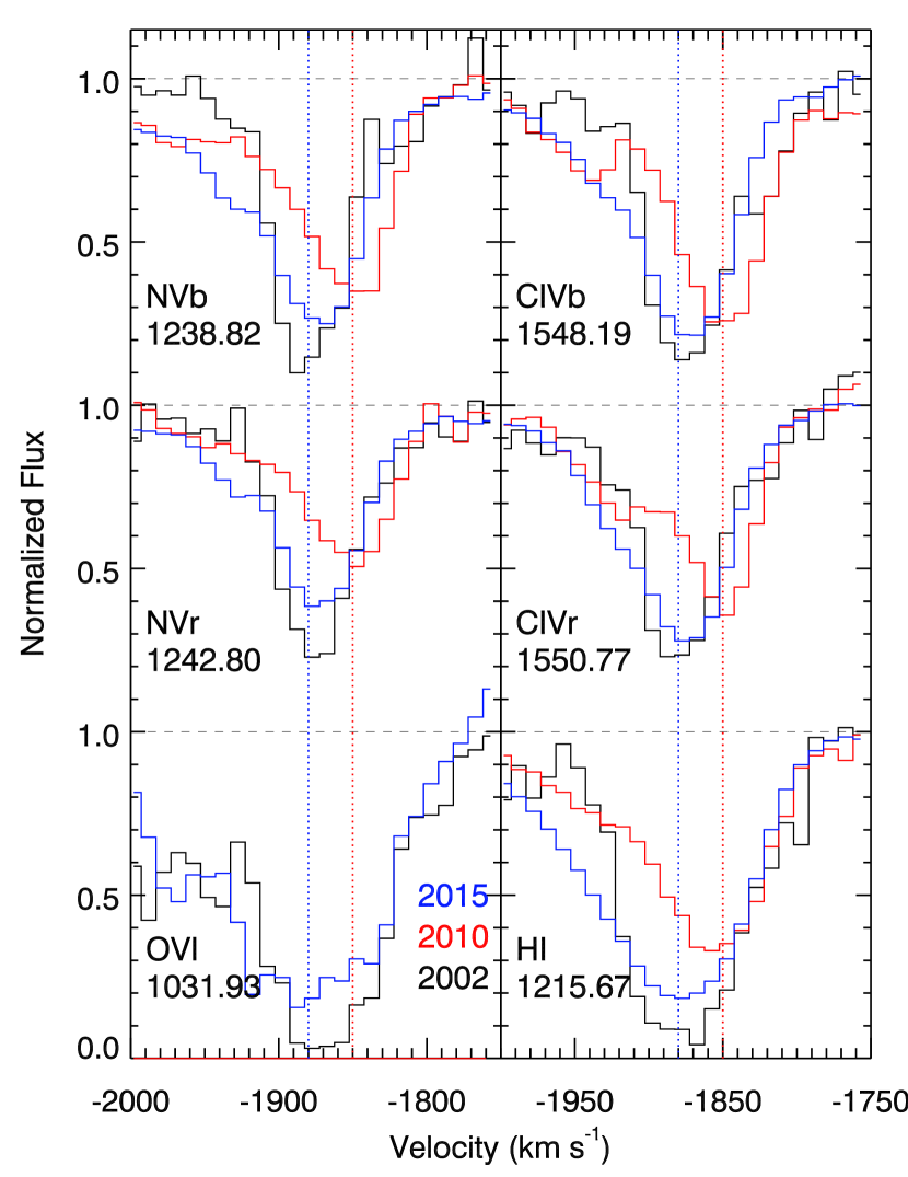
Figure 6: Component 3 variations: normalized spectrum showing the velocity-shift anomaly in the 2010 epoch. We illustrate this anomaly in outflow component 3 by showing vertical dotted lines through the centroid of the absorption troughs in the 2002 and 2015 epochs (blue) and during the 2010 epoch (red). We note that the overall depth of component 3 is lowest in the 2010 epoch in all of the observed troughs.

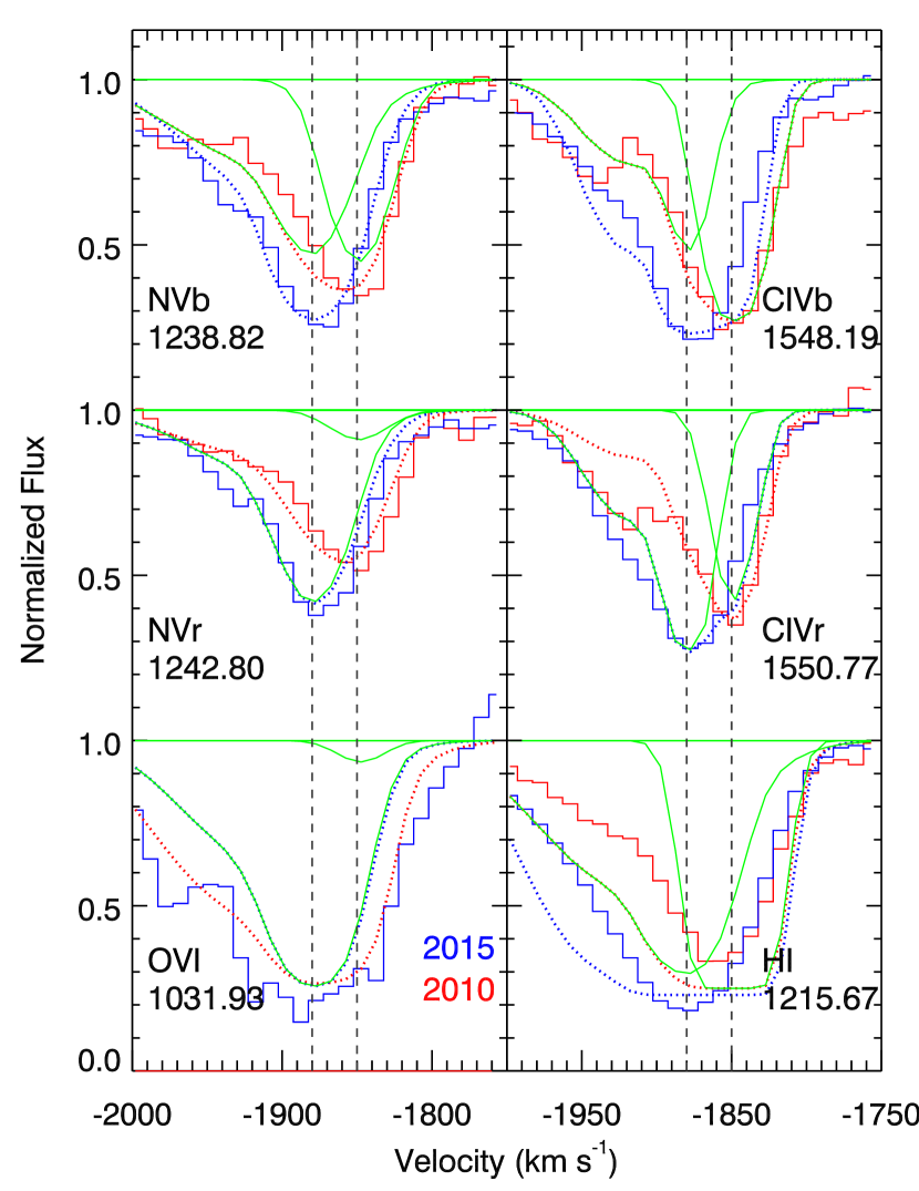
Figure 7: Model fit for troughs variation in component 3 (see § 4.3.2). The normalized data is shown in red for the 2010 epoch and blue for the 2015 one. The full model for each trough is shown by the dotted lines of the same color. In green we show the contribution of component 3a (left curve) and 3b (right curve). For the blue doublet components (left panels) we show the contribution of the 2 phases to the 2010 model, and for the red doublet components (right panels) we show the contribution of the 2 phases to the 2015 model.

The key for understanding this unusual behavior of component 3 comes from taking into account the UV flux level in the different epochs. As can be seen in Table 2, the UV flux during the 2010 observations was the highest of all epochs, roughly twice the flux of the 2002 and 2015 epochs, and 5 times higher than the 2004 epoch. We therefore attempt to model the trough variations using the variation in the photoionization equilibrium induced by the changes in UV flux between the epochs. We note that such a model can, in principle, match most of the trough variations. However, there must be other effects as well. For example, while the high velocity wing changes uniformly between the 2010 and 2005 epochs in all of the troughs, the 2002 epoch is deeper close to the centroid and shallower at the high velocity wing. This 3-epoch comparative phenomenology cannot be explained by pure photoionization changes.

A model based on a single ionization phase for component 3 is inadequate for this purpose, as it predicts a uniform change in a trough’s depth across the entire profile. We therefore attempt to model component 3 with two ionization phases whose velocity centroid is shifted by 30 km s^-1 relative to each other. Our approach is to build the simplest possible two-phase model that can fit the major empirical behavior seen in the data. Following this principle, we construct a model that has two kinematic components (3a and 3b) that differ by a constant $\Delta$$U_{\mathrm{\scriptscriptstyle H}}$, and the individual $U_{\mathrm{\scriptscriptstyle H}}$ values change linearly with the measured UV flux in each epoch. The model assumes the same super-solar abundances we used in modelling component 1 and in the photoionization solution for component 3 (see bottom panel of Figure 5). We further assume that a simple constant covering factor is applicable for all the ionic troughs ($C(v)=0.75$). Below we give more details for this model and describe its successes and shortcomings.

We modeled component 3a with two Gaussian optical-depth profiles. The velocity centroid of the main Gaussian is at –1880 km s^-1 and its width is $\sigma=20$ km s^-1. The high velocity wing was modeled with a Gaussian centered at –1920 km s^-1 and width of $\sigma=50$ km s^-1. Component 3b was modeled with a Gaussian centered at –1850 km s^-1 and width of $\sigma=15$ km s^-1. As seen in Figure 6, the trough shapes in 2002 and 2015 are quite similar when the UV flux differed by only 34%. However, large changes are observed between the 2015 and the 2010 epochs, where there is a factor of 2.6 change in the UV flux. Therefore, in Figure 7, we show the best fit results for only the 2010 and 2015 data.

The main success of this model is the good match for the eight data sets for the C iv and N v troughs (for each ion we fit both doublet components for two epochs: 2010, 2015). This is done with a simple optical depth model where the changes are due to a difference in the ionization parameter of the absorber that equal the flux change between the epochs.

A reasonable match for the O vi doublet profile in 2015 is obtained using the same parameters that fit the C iv and N v troughs (The O vi spectral region was not observed in 2010). Quantitatively, the model optical depth is smaller than the data’s optical depth by up to 50% across the trough. The Ly$\alpha$ fit shows similar behavior in the high velocity wing, and an opposite behavior (model deeper than data) in the low velocity wing. However, it is clear that the AOD assumption for the low velocity wing of Ly$\alpha$ is incorrect as the trough does not change in that region between the epochs. The most probable explanation for that is a strong saturation of the Ly$\alpha$ trough in that velocity region with a velocity dependent covering factor (e.g., Arav et al. 2008). Another weakness in the model is that, unlike the model for component 1, the best fit model for component 3 invokes changes in $N_{\mathrm{\scriptscriptstyle H}}$ for components 3a and 3b by up to a factor of two between the 2010 and 2015 epochs (see Figure 5).

In summary, most of the troughs’ variability in component 3 can be explained by photoionization reaction of two sub components to the quantitative changes in incident ionizing flux, especially the observed back and forth velocity shift of the trough centroid. However, an AOD model with a constant covering factor is inadequate for two reasons. 1) The Ly$\alpha$ trough shows moderate saturation and a velocity dependent covering factor. 2) In 2002, all 5 troughs from C iv, N v and Ly$\alpha$ have a deeper core but shallower high velocity wing (at $v<-1920$ km s^-1) than the same troughs in the 2010 and 2015 epochs. This behavior is incompatible with pure photoionization changes, as the core and the wing are expected to show depth changes in the same direction.

4.3.3 Distance determination from trough variability

The behavior of component 3’s troughs during the 2015 campaign in response to UV flux variation is more complicated than that of component 1. Different portions of the trough behave in different ways. All 4 troughs from C iv and N v, as well as Ly$\alpha$ show trough variation between the June (visit 1) and November (visit 2) 2015 epochs, but only over the narrow velocity range –1910 to -1950 km s^-1(on the high velocity wing of the trough). The other portions of the troughs (full span –1800 to –2070 km s^-1) do not show variability over this time period. It is plausible that this behavior is the result of combining moderate saturation across most of the trough with relatively small UV flux changes (a 28% decrease between visits 1 and 2, see Table 3). Qualitatively, such a model explains: a) why no variability is observed between the later epochs where the flux changes are less than 16%; b) why the entire trough changes between the 2010 and the 2015b epochs (flux change by a factor of 2.6).

The varied response of component 3 to flux variation complicates the extraction of a photoionization time-scale from the data. It is clear that the entire trough shows trough changes correlated with large flux change on a 5 year time scale (between the 2010 and 2015 epochs), while small portions of the trough show such changes on a 6 month timescale (between visits 1 and 2 in 2015). Similar to our time-dependent photoionization analysis of component 1, this allows us to derive log$(n_{\mathrm{\scriptscriptstyle e}})>2.8$ (cm^-3) or log$(n_{\mathrm{\scriptscriptstyle e}})>3.6$ (cm^-3) using the 5 years and 6 months timescales, respectively. For these estimates, we used the N v variations, which yields the highest $n_{\mathrm{\scriptscriptstyle e}}$ for the initial conditions given by the photoionization solution for component 3.

In turn, these $n_{\mathrm{\scriptscriptstyle e}}$ lower limits yield a maximum distance for component 3 of 150 pc or 60 pc for the 5 years and 6 months time-scales, respectively (where we used the $U_{\mathrm{\scriptscriptstyle H}}$ value of the global solution for component 3, see Figure 5).

5 Comparison with the X-ray results

As mentioned in section 1, we observed the X-ray manifestation of the outflow with both XMM-Newton and Chandra. Analysis results for the The X-ray and UV troughs occupy roughly the same velocity range $-2100<v<-400$ km s^-1, see Table 2 here for the UV, Figure 3 in Peretz et al. (2018) for the XMM-Newton RGS observations, and Table 3 in Mehdipour et al. (2018) for the Chandra HETG observations.

HST/COS UV data are sensitive to much smaller ionic column densities ($N_{ion}$) than the XMM/RGS X-ray data. For NGC 7469, the measured UV CNO $N_{ion}$ are two to three orders of magnitude lower than the secured CNO $N_{ion}$ measurements in the X-ray. As shown in section 4, the Ly$\alpha$ and CNO UV troughs are not heavily saturated. Therefore, we expect the $N_{\mathrm{\scriptscriptstyle H}}$ of the UV phase to be roughly two orders of magnitude smaller than the X-ray phase.

For the 2015b epoch, we found for component 1 $\log(N_{\mathrm{\scriptscriptstyle H}})\approx 18.3$ (cm^-2) and $\log(U_{\mathrm{\scriptscriptstyle H}})\approx-1.0$; and for component 3 $\log(N_{\mathrm{\scriptscriptstyle H}})\approx 18.8$ (cm^-2) and $\log(U_{\mathrm{\scriptscriptstyle H}})\approx-1.8$ (see Figures 3 and 5). For the secured CNO $N_{ion}$ measurements in the X-ray, the minimum $\log(N_{\mathrm{\scriptscriptstyle H}})$ is between 20–21.3 (cm^-2), with a spread of $\log(U_{\mathrm{\scriptscriptstyle H}})$ between –0.5 and +0.3.

These results are in accordance with the expectations outlined in the above paragraph (even when we take into account the super solar metallicity found for the UV material). Accounting for the super-metallicity of the UV photoionization solution, we conclude that in the NGC 7469 outflow, the $N_{\mathrm{\scriptscriptstyle H}}$ of the UV material is only about 10% and 0.5% of the $N_{\mathrm{\scriptscriptstyle H}}$ of the low and high X-ray ionization phases, respectively (see Figure 6 in Peretz et al. 2018). There is no contradiction between the UV and X-ray results, as the UV data sample material with lower $U_{\mathrm{\scriptscriptstyle H}}$ values than even the low ionization X-ray phase. We note that based on X-ray troughs from ions of Ne, Mg, S and Fe, most of the outflow’s $N_{\mathrm{\scriptscriptstyle H}}$ ($\sim 10^{22}$ cm^-2) arises from a much higher ionization phase with $\log(U_{\mathrm{\scriptscriptstyle H}})$ between $+0.5$ and $+2$ (see Peretz et al. 2018; Mehdipour et al. 2018).

The UV and X-ray estimates for the distance of the outflow from the central source ($R$) are in agreement and complementary. UV Component 3, which carries most of the $N_{\mathrm{\scriptscriptstyle H}}$ of the UV phase, has an upper limit of 150 pc or 60 pc (see section 4.3.3). This is consistent with the X-ray warm absorber lower limits for $R$ of 12 pc or 31 pc (Peretz et al. 2018).

Assuming the same distance and velocities for the UV and X-ray outflows, we note that the kinetic luminosity of the UV outflowing material will be negligible compared to that of the X-ray component. This is due to the fact that the kinetic luminosity is proportional to the total column density (see equations 5-7, and accompanied discussion in Borguet et al. 2012). Therefore, since the X-ray phase has a hundred times larger $N_{\mathrm{\scriptscriptstyle H}}$, it will carry a hundred times larger kinetic luminosity.

6 Summary

Our multiwavelength campaign on NGC 7469 yielded deep insights about the physical characteristics of this AGN outflow. The UV analysis described in this paper focused on the two major UV absorption components, 1 and 3.

Component 1 at $\sim-550$ km s^-1  is close to being optically thin in all its troughs, and shows simple photoionization response to changes in the incident ionizing flux. This behavior allowed us to extract a clear physical picture of the absorber:

1. The outflowing gas must have about twice proto-solar metallicity. This is similar to our findings for the outflow in Mrk 279 (Arav et al. 2007).

2. A simple model based on a fixed total column-density absorber, reacting to changes in ionizing illumination, matches the observed trough changes in all epochs. This is similar to our findings for outflow component 1 in NGC 5548 (Arav et al. 2015).

3. The simple response to changes of the incident ionizing flux allows us to use time-dependent photoionization analysis and obtain a distance of $R=6^{+2.5}_{-1.5}$ pc from the central source.

Component 3 at $\sim-1880$ km s^-1 shows a more complicated behavior: a) Some of its troughs are moderately saturated. b) It shows a complex variability pattern where the velocity centroid shifts by +30 km s^-1 in 2010 compared to the 2002 and 2004 epochs, but shifts to its original position in 2015. A model based on two sub-components reacting to photoionization changes is partially successful in explaining this behavior. Using time-dependent photoionization analysis we are able to put an upper limit on its distance $R$ between 60 and 150 pc.

Comparing the physical picture that emerges from the UV analysis to that of the X-ray data we find:

1. The total column density of the UV phase is roughly 1% and 0.1% of the lower and upper ionization components of the warm absorber, respectively. There is no contradiction here as even the lower ionization X-ray component has a significantly higher $U_{\mathrm{\scriptscriptstyle H}}$ value than those inferred for the UV components.

2. The lower limit on the distance inferred for the X-ray phase is compatible with the upper limits inferred for UV component 3 (that has 3 times higher $N_{\mathrm{\scriptscriptstyle H}}$ than component 1). Together they suggest that the bulk of the outflow in somewhere between 12 and 150 pc from the central source.

Finally, we note that the radial-velocity of all three components is larger than the escape speed at their distance from the AGN. For the $1.2\times 10^{7}$ solar masses black-hole in NGC 7469 (Peterson 2014), the escape speed for component 1 at $R=6$ pc, is $\sim 130$ km s^-1 while its radial velocity is $\sim 500$ km s^-1. Components 2 and 3 are farther away and have higher radial velocities so their velocities are definitely larger than their escape velocity, even if at their distances the enclosed mass is dominated by the galaxy. Thus, it is clear that all 3 components are not bound to the gravitational field of the central black-hole.

Acknowledgments. This work was supported by NASA grant NNX16AC07G through the XMM-Newton Guest Observing Program, and through grants for HST program number 14054 from the Space Telescope Science Institute, which is operated by the Association of Universities for Research in Astronomy, Incorporated, under NASA contract NAS5-26555. The research at the Technion is supported by the I-CORE program of the Planning and Budgeting Committee (grant number 1937/12). E.B. received funding from the European Union’s Horizon 2020 research and innovation program under the Marie Sklodowska- Curie grant agreement No. 655324. SRON is supported financially by NWO, The Netherlands Organization for Scientific Research. N.A. is grateful for a visiting-professor fellowship at the Technion, granted by the Lady Davis Trust. S.B. and M.C. acknowledge financial support from the Italian Space Agency under grant ASI-INAF I/037/12/0. B.D.M. acknowledges support from the European Union’s Horizon 2020 research and innovation program under the Marie Skłodowska-Curie grant agreement No. 665778 via the Polish National Science Center grant Polonez UMO-2016/21/P/ST9/04025. L.D.G. acknoweledges support from the Swiss National Science Foundation. G.P. acknowledges support by the Bundesministerium für Wirtschaft und Technologie/Deutsches Zentrum fur Luft- und Raumfahrt (BMWI/DLR, FKZ 50 OR 1715 and FKZ 50 OR 1812) and the Max Planck Society. P.O.P. acknowledges support from CNES and from PNHE of CNRS/INSU. BDM acknowledges support from the European Union’s Horizon 2020 research and innovation programme under the Marie Skłodowska- Curie grant agreement No. 798726

References

- Arav et al. (2013) Arav, N., Borguet, B., Chamberlain, C., Edmonds, D., & Danforth, C. 2013, MNRAS, 436, 3286
- Arav et al. (2015) Arav, N., Chamberlain, C., Kriss, G. A., et al. 2015, A&A, 577, A37
- Arav et al. (2012) Arav, N., Edmonds, D., Borguet, B., et al. 2012, A&A, 544, A33
- Arav et al. (2007) Arav, N., Gabel, J. R., Korista, K. T., et al. 2007, ApJ, 658, 829
- Arav et al. (2005) Arav, N., Kaastra, J., Kriss, G. A., et al. 2005, ApJ, 620, 665
- Arav et al. (2018) Arav, N., Liu, G., Xu, X., et al. 2018, ApJ, 857, 60
- Arav et al. (2008) Arav, N., Moe, M., Costantini, E., et al. 2008, ApJ, 681, 954
- Behar et al. (2017) Behar, E., Peretz, U., Kriss, G. A., et al. 2017, A&A, 601, A17
- Blustin et al. (2007) Blustin, A. J., Kriss, G. A., Holczer, T., et al. 2007, A&A, 466, 107
- Blustin et al. (2003) Blustin, A. J. et al. 2003, A&A, 403, 481
- Borguet et al. (2013) Borguet, B. C. J., Arav, N., Edmonds, D., Chamberlain, C., & Benn, C. 2013, ApJ, 762, 49
- Borguet et al. (2012) Borguet, B. C. J., Edmonds, D., Arav, N., Dunn, J., & Kriss, G. A. 2012, ApJ, 751, 107
- Ciotti et al. (2010) Ciotti, L., Ostriker, J. P., & Proga, D. 2010, ApJ, 717, 708
- Costantini et al. (2007) Costantini, E., Kaastra, J. S., Arav, N., et al. 2007, A&A, 461, 121
- Debes et al. (2016) Debes, J., et al., et al., et al., & et al. 2016, Cosmic Origins Spectrograph Instrument Handbook, Version 8.0 (Baltimore), 300
- Faucher-Giguère et al. (2012) Faucher-Giguère, C.-A., Quataert, E., & Murray, N. 2012, MNRAS, 420, 1347
- Ferland et al. (2017) Ferland, G. J., Chatzikos, M., Guzmán, F., et al. 2017, Rev. Mexicana Astron. Astrofis., 53, 385
- Gabel et al. (2006) Gabel, J. R., Arav, N., & Kim, T. 2006, ApJ, 646, 742
- Gabel et al. (2003) Gabel, J. R., Crenshaw, D. M., Kraemer, S. B., et al. 2003, ApJ, 583, 178
- Gabel et al. (2005) Gabel, J. R., Kraemer, S. B., Crenshaw, D. M., et al. 2005, ApJ, 631, 741
- Green et al. (2012) Green, J. C., Froning, C. S., Osterman, S., et al. 2012, ApJ, 744, 60
- Hamann & Ferland (1993) Hamann, F. & Ferland, G. 1993, ApJ, 418, 11
- Hopkins & Elvis (2010) Hopkins, P. F. & Elvis, M. 2010, MNRAS, 401, 7
- Kaastra et al. (2012) Kaastra, J. S., Detmers, R. G., Mehdipour, M., et al. 2012, A&A, 539, A117
- Kaastra et al. (2014) Kaastra, J. S., Kriss, G. A., Cappi, M., et al. 2014, Science, 345, 64
- Kaastra et al. (2011) Kaastra, J. S. et al. 2011, A&A, 534, A36
- Kriss et al. (2003) Kriss, G. A., Blustin, A., Branduardi-Raymont, G., et al. 2003, A&A, 403, 473
- Kriss et al. (2011) Kriss, G. A. et al. 2011, A&A, 534, A41
- Lodders et al. (2009) Lodders, K., Palme, H., & Gail, H.-P. 2009, in ”Landolt-Börnstein - Group VI Astronomy and Astrophysics Numerical Data and Functional Relationships in Science and Technology Volume, ed. J. E. Trümper, 44
- Mehdipour et al. (2011) Mehdipour, M., Branduardi-Raymont, G., Kaastra, J. S., et al. 2011, A&A, 534, A39
- Mehdipour et al. (2018) Mehdipour, M., Kaastra, J. S., Costantini, E., et al. 2018, A&A, 615, A72
- Middei et al. (2018) Middei, R., Bianchi, S., Cappi, M., et al. 2018, ArXiv e-prints
- Ostriker et al. (2010) Ostriker, J. P., Choi, E., Ciotti, L., Novak, G. S., & Proga, D. 2010, ApJ, 722, 642
- Peretz et al. (2018) Peretz, U., Behar, E., Kriss, G. A., et al. 2018, A&A, 609, A35
- Peterson (2014) Peterson, B. M. 2014, Space Sci. Rev., 183, 253
- Scott et al. (2005) Scott, J. E., Kriss, G. A., Lee, J. C., et al. 2005, ApJ, 634, 193
- Soker & Meiron (2011) Soker, N. & Meiron, Y. 2011, MNRAS, 411, 1803
- Steenbrugge et al. (2005) Steenbrugge, K. C., Kaastra, J. S., Crenshaw, D. M., et al. 2005, A&A, 434, 569
- Wilson et al. (1991) Wilson, A. S., Helfer, T. T., Haniff, C. A., & Ward, M. J. 1991, ApJ, 381, 79