Implications of the search for optical counterparts during the first six months of the Advanced LIGO’s and Advanced Virgo’s third observing run: possible limits on the ejecta mass and binary properties

Abstract

GW170817 showed that neutron star mergers not only emit gravitational waves but also can release electromagnetic signatures in multiple wavelengths. Within the first half of the third observing run of the Advanced LIGO and Virgo detectors, there have been a number of gravitational wave candidates of compact binary systems for which at least one component is potentially a neutron star. In this article, we look at the candidates S190425z, S190426c, S190510g, S190901ap, and S190910h, predicted to have potentially a non-zero remnant mass, in more detail. All these triggers have been followed up with extensive campaigns by the astronomical community doing electromagnetic searches for their optical counterparts; however, according to the released classification, there is a high probability that some of these events might not be of extraterrestrial origin. Assuming that the triggers are caused by a compact binary coalescence and that the individual source locations have been covered during the EM follow-up campaigns, we employ three different kilonova models and apply them to derive possible constraints on the matter ejection consistent with the publicly available gravitational-wave trigger information and the lack of a kilonova detection. These upper bounds on the ejecta mass can be related to limits on the maximum mass of the binary neutron star candidate S190425z and to constraints on the mass-ratio, spin, and NS compactness for the potential black hole-neutron star candidate S190426c. Our results show that deeper electromagnetic observations for future gravitational wave events near the horizon limit of the advanced detectors are essential.

1 Introduction

By the combined detection of GW170817, AT2017gfo, and GRB170817A, the field of multi-messenger astronomy was ushered into a new era in which gravitational-wave (GW) and electromagnetic (EM) signatures are simultaneously measured and analyzed, e.g., Abbott B. P. (2017); Abbott et al. (2017b); Arcavi et al. (2017); Coulter et al. (2017); Lipunov et al. (2017); Mooley et al. (2017); Savchenko et al. (2017); Soares-Santos et al. (2017); Tanvir et al. (2013); Troja et al. (2017); Valenti et al. (2017). Joint analyses allow a better understanding of the supranuclear-dense matter inside neutron stars (NSs) (e.g. Radice et al. (2018); Radice & Dai (2019); Bauswein et al. (2017); Margalit & Metzger (2017); Rezzolla et al. (2018); Coughlin et al. (2018b); Coughlin et al. (2018a); Capano et al. (2019)), a precise measurement of the speed of gravitational waves (Abbott et al., 2017c), an independent measurement of the expansion rate of the Universe (Abbott et al., 2017a; Hotokezaka et al., 2019; Coughlin et al., 2019a; Dhawan et al., 2019), and constraints on alternative models of gravity (Ezquiaga & Zumalacárregui, 2017; Baker et al., 2017; Creminelli & Vernizzi, 2017; Sakstein & Jain, 2017).

In general, the merger of two compact objects from which at least one is a NS, is connected to a variety of possible EM signatures in almost all wavelengths. A highly relativistic jet can produce a short gamma-ray burst (sGRB) lasting a few seconds (Eichler et al., 1989; Paczynski, 1991; Narayan et al., 1992; Mochkovitch et al., 1993; Lee & Ramirez-Ruiz, 2007; Nakar, 2007) and a synchrotron afterglow in the X-rays, optical and radio visible bands for hours to months after the initial emission due to the deceleration of the jet into the ambient media (Sari et al., 1998). The ejection of highly neutron rich material, being the seed of r-process elements (Lattimer & Schramm, 1974, 1976), powers a thermal ultraviolet/optical/near-infrared kilonova due to the radioactive decay of the new heavy elements produced in the ejecta (Li & Paczynski, 1998; Metzger et al., 2010; Roberts et al., 2011; Kasen et al., 2017). Although the color and luminosity of a kilonova will be viewing angle dependent, the kilonova signature is, in contrast to the sGRB and its afterglow, likely visible from all viewing angles. This means that after every merger which ejects a sufficient amount of material, one should be able to observe a kilonova regardless of the orientation of the system (Roberts et al., 2011). Thus, kilonovae provide a smoking guns evidence for binary neutron star (BNS) and black hole - neutron star (BHNS) mergers.

However, current numerical relativity studies indicate that not all BNS or BHNS collisions will eject enough material to create EM signals as bright as the one observed for GW170817. For most BNS systems, the EM signals are expected to be dimmer than for GW170817 if a black hole (BH) forms directly after the moment of merger, since for these prompt collapse configurations the amount of ejected material and the mass of the potential debris disk is expected to be very small. Whether a merger remnant undergoes a prompt collapse depends mostly on its total mass (Bauswein et al., 2013; Hotokezaka et al., 2013; Dietrich & Ujevic, 2017; Köppel et al., 2019; Agathos et al., 2019) but also seems to be sub-dominantly affected by the mass-ratio (Kiuchi et al., 2019). For highly asymmetric mass ratios ($m_{1}/m_{2}\lesssim 0.8$), there could be a non-negligible ejecta mass and/or a massive accretion disk around the black hole remnant even for prompt collapse scenarios (Kiuchi et al., 2019).

In the case of a BHNS system, the brightness of the potential EM counterpart depends on whether the NS gets tidally disrupted by the BH and, thus, ejects a large amount of material and forms a massive accretion disk; or if the star falls into the BH without disruption, preventing the production of GRBs and kilonovae. Thus, the outcome of the merger is mostly determined by the mass ratio of the binary, the spin of the black hole, and the compactness of the NS, with disruption being favored for low-mass, rapidly rotating BH and large NS radii (Etienne et al., 2009; Pannarale et al., 2011; Foucart, 2012; Kyutoku et al., 2015; Kawaguchi et al., 2016; Foucart et al., 2018).

Since the beginning of the third observation run, a number of potential GW events have triggered extensive follow-up campaigns to search for possible EM counterparts, most notably S190425z (LIGO Scientific Collaboration & Virgo Collaboration, 2019a, b), S190426c (LIGO Scientific Collaboration & Virgo Collaboration, 2019c, s), S190510g (LIGO Scientific Collaboration & Virgo Collaboration, 2019f), S190814bv (LIGO Scientific Collaboration & Virgo Collaboration, 2019o), S190901ap (LIGO Scientific Collaboration & Virgo Collaboration, 2019t), S190910h (LIGO Scientific Collaboration & Virgo Collaboration, 2019w), S190910d (LIGO Scientific Collaboration & Virgo Collaboration, 2019v), S190923y (LIGO Scientific Collaboration & Virgo Collaboration, 2019z), and S190930t (LIGO-Virgo collaboration, 2019); cf. Tab. 1 for more details. The large size of localization regions with thousands of square degrees have proved much more challenging to cover over short times than the $\sim 20$ square degrees of GW170817. In fact, no joint detection of GW and EM signals have been confirmed; see also Dado & Dar (2019) for a possible explanation that no sGRBs has been observed for the GW events within O3a. While a detection of an EM signature will help significantly to unravel some of the remaining open questions related to compact binary mergers, the possibility of a “missing” EM signature for an astrophysical relevant trigger whose sky location was covered during an EM follow-up campaign also delivers some information about the source properties, as we will discuss.

Table 1: Overview about officially non-retracted GW triggers with large probabilities to be BNS or BHNS systems. The individual columns refer to: the name of the event, an estimate using the most up-to-date classification for the event to be a BNS [p(BNS)], a BHNS [p(BHNS)], or terrestrial noise [p(terrestrial)] (Kapadia et al., 2019), and an indicator to estimate the probability of producing EM signature considering the candidate with astrophysical origin [p(HasRemnant)], whose definition is in the LIGO-Virgo alert userguide. Note that the alert can be also classified as “MassGap,” completing the possible classifications. Note that within our analysis, we do not consider S190718y because of its very low probability to be of astrophysical origin.

Name	p(BNS)	p(BHNS)	p(terr.)	p(HasRemn.)
S190425z	$>99\%$	$0\%$	$<1\%$	$>99\%$
S190426c	$24\%$	$6\%$	$58\%$	$>99\%$
S190510g	$42\%$	$0\%$	$58\%$	$>99\%$
S190718y∗	$2\%$	$0\%$	$98\%$	$>99\%$
S190814bv	$0\%$	$>99\%$	$<1\%$	$<1\%$
S190901ap	$86\%$	$0\%$	$14\%$	$>99\%$
S190910d	$0\%$	$98\%$	$2\%$	$<1\%$
S190910h	$61\%$	$0\%$	$39\%$	$>99\%$
S190923y	$0\%$	$68\%$	$32\%$	$<1\%$
S190930t	$0\%$	$74\%$	$26\%$	$<1\%$

In this article, we try to understand if from the detection or, more likely, non-detection of an EM counterpart to a potential GW event it is possible to place constraints on the merger outcome and the properties of the system. For this purpose, we will shortly summarize the EM follow-up campaigns of S190425z, S190426c, S190510g, S190814bv, S190901ap, S190910d, S190910h, S190923y, and S190930t in Sec. 2. We further also refer to Andreoni et al. (2019a) for a dedicated discussion done by the GROWTH collaboration about S190814bv.

In Sec. 3 we focus on the events for which the HasRemnant prediction provides a high probability of a potential EM signature (S190425z, S190426c, S190510g, S190901ap, and S190910h); cf. Tab. 1. Under the assumption that the GW candidate location was covered during the EM observations, we will use a set of three different lightcurve models (Kasen et al., 2017; Bulla, 2019; Hotokezaka & Nakar, 2019) to predict the properties of the kilonova consistent with the non-observation of an EM counterpart. This analysis allows us to derive constraints on the maximum ejecta mass for each event in Sec. 3 and connects our findings to the binary properties in Sec. 4. These constraints are typically not very striking given the large distance to the GW triggers in the first half of advanced LIGO and advanced Virgo’s third observing run, which highlights that, if possible, longer exposure times should be employed to reduce the possibility that interesting transients might be missed. We summarize our conclusions and lessons learned for observations in the second half of the third observing run in Sec. 5.

2 EM follow-up campaigns

We summarize the EM follow-up work of the various teams that performed synoptic coverage of the sky localization area and who have circulated their findings in publicly available circulars during the first six months of the third observing run. For a summary of the follow-up campaign during the second observing run, please see Abbott B.P. (2019) and references therein. We differentiate the candidates by their classification (predominantly BNS in Table 2 and predominantly BHNS in Table 3). While this is mostly an initial classification and may change based on future offline estimates, we think it is useful as, for example, the distance estimates tend to be different between these classes. A short discussion about each candidate is presented below; note that we do not report the observations that exclusively target galaxies.

2.1 S190425z

LIGO/Virgo S190425z was identified by the LIGO Livingston Observatory (L1) and the Virgo Observatory (V1) at 2019-04-25 08:18:05.017 UTC (LIGO Scientific Collaboration & Virgo Collaboration, 2019a, b). LIGO Hanford Observatory (H1) was not taking data at the time. It has been so far categorized as a BNS signal, reported as a BNS $(99\%)$ with a small probability of being in the mass gap $(<1\%)$. Due to the low signal-to-noise ratio (SNR) in V1, S190425z’s sky localization is relatively poor, covering nearly $10,000$ square degrees. The original distance quoted for this system is $155\pm 45$ Mpc, thus, about $\sim 4$ times further away than GW170817.

As the first alert during the O3 campaign with a high probability of having a counterpart, there was an intense follow-up campaign within the first $\sim$ 72 hours after the initial notice (see $\approx$ 120 reports in GCN archive, mostly focusing on optical follow-up). As expressed in Cook et al. (2019), with more than 50,000 galaxies compatible with the 90% sky area volume due to the large uncertainty of the localization, it was difficult to fully cover S190425z’s localization. However, as shown in Table 2, ten telescopes reported tiling observations of the localization. For example, both the Zwicky Transient Facility (ZTF) (Bellm et al., 2018; Graham et al., 2019; Dekany et al., 2019; Masci et al., 2018), a camera and associated observing system on the Palomar 48 inch telescope, and Palomar Gattini-IR, a new wide-field near-infrared survey telescope at Palomar observatory, followed up S190425c extensively (Coughlin et al., 2019b). Covering about 8000 and 2200 square degrees respectively, the systems achieved depths of $\approx$ 21 $m_{\textrm{AB}}$ in g- and r-bands with ZTF and 15.5 mag in J-band with Gattini-IR. Among them, using the LALInference skymap, about 21% of and 19% of the sky localization was covered by ZTF and Palomar Gattini-IR respectively. In addition, Pan-STARRS covered 28% of the bayestar sky localization area in g-band with a limiting magnitude of $i=21.5$ mag (Smith et al., 2019); similarly, GOTO covered 30% of the initial skymap down to $L=20.5$ mag (Steeghs et al., 2019a).

2.2 S190426c

LIGO/Virgo S190426c was identified by H1, L1, and V1 at 2019-04-26 15:21:55.337 UTC (LIGO Scientific Collaboration & Virgo Collaboration, 2019c, s). With a probability of 58% to be terrestrial, S190426c might not be of astrophysical origin. But assuming that the signal is of astrophysical relevance, S190426c seems to be a BHNS system with relative probabilities of approximately 12 : 5 : 3 : 0 for the categories NSBH : MassGap : BNS : BBH, respectively (LIGO Scientific Collaboration & Virgo Collaboration, 2019e). Within this analysis the HasRemnant probability is stated as $72\%$, thus, for all events with large HasRemnant predictions, is our best example for a possible BHNS merger. S190426c’s sky localization, given that it was discovered by multiple interferometers, covers less area than S190425z. The initial 90% credible region was 1260 deg² with a luminosity distance of $375\pm 108$ Mpc (LIGO Scientific Collaboration & Virgo Collaboration, 2019c). The updated skymap, sent 48 hrs after the initial skymap, had a 90% credible region of 1130 deg² and a luminosity distance estimate of $377\pm 100$ Mpc (LIGO Scientific Collaboration & Virgo Collaboration, 2019d). As the first event announced with a significant probability of a BHNS nature, the interest in this event was large and about 70 circulars have been sent out (see the GCN archive). As shown in Table 3, 13 telescopes scanned the localization region; for example, ASAS-SN (Shappee et al., 2019), GOTO (Steeghs et al., 2019b), and ZTF (Kasliwal et al., 2019b) covered more than 50% of the sky localization area using multiple filters in the first 48 hrs.

2.3 S190510g

LIGO/Virgo S190510g was identified by H1, L1 and V1 at 2019-05-10 02:59:39.292 UTC (LIGO Scientific Collaboration & Virgo Collaboration, 2019f). S190510g’s latest sky localization covers 1166 deg² with a luminosity distance of $227\pm 92$ Mpc (LIGO Scientific Collaboration & Virgo Collaboration, 2019g). In the most recent update provided by the LIGO and Virgo Collaboration, the event is now more likely caused by noise (LIGO Scientific Collaboration & Virgo Collaboration, 2019h) than it is to be an astrophysical source, with a probability of terrestrial (58%) and BNS (42%); however, since the event is, up to now, not officially retracted, we will consider it in this article. Due to its potential BNS nature and its trigger time being close to the beginning of the night in the Americas, the event was followed-up rapidly, with about 60 circulars produced (see GCN archive). With $\sim$ 65% coverage of the LALInference skymap, GROWTH-DECam realized the deepest follow-up (Andreoni et al., 2019b). We can compute the joint coverage of different telescopes based upon their pointings and field of view reporting in the GCNs. Within 24 hr, CNEST, HMT, MASTER, Xinglong and TAROT, all with clear filters down to 18 mag, observed 71% of the LALInference sky localization area; this number would assuredly be higher with a coordinated effort.

2.4 S190814bv

The candidate S190814bv was identified by H1, L1, and V1 on 2019-08-14 21:10:39.013 UTC. First classified as a compact merger with one component having an initial mass between 3 and 5 solar masses (LIGO Scientific Collaboration & Virgo Collaboration, 2019o), the candidate is now classified as a BHNS with posterior support from parameter estimation (Veitch et al., 2015) with NSBH ($>$99%) (LIGO Scientific Collaboration & Virgo Collaboration, 2019p). Initially, two different Bayestar-based sky localizations were generated, one with the lower false alarm rate which included Livingston and Virgo data (sent 21 min after the trigger time) and one with contribution of the three instruments (sent 2 hr after the GW trigger time). A third skymap (LALInference) with all three interferometers was sent $\sim$ 13.5 hr after the trigger time. The initial three interferometer 90% credible region was 38 deg² with a luminosity distance estimated at $276\pm 56$ Mpc. The latest 90% credible region is 23 deg² with a luminosity distance of $267\pm 52$ Mpc. With the small localization region, and its location in the Southern hemisphere, the event was ideal for follow-up. However, no counterpart candidates remain after the extensive follow-up, with about 70 circulars produced (see GCN archive). As shown in Table 3, many survey systems covered a vast majority of the localization region, including ATLAS (Srivastav et al., 2019), DESGW-DECam (Soares-Santos et al., 2019), and TAROT (Klotz et al., 2019). We note here despite the small sky area and the intensive followed-up studies, we do not consider this object in the analysis due to its HasRemnant value.The joint coverage of MASTER and TAROT with 17 mag in clear filter within the first 3 hours was about 90% of the LALinference skymap.

2.5 S190901ap

LIGO/Virgo S190901ap was identified by L1 and V1 at 2019-09-01 23:31:01.838 UTC (LIGO Scientific Collaboration & Virgo Collaboration, 2019t). The candidate is currently classified as BNS (86%) and terrestrial (14%). The latest 90% credible region is 14753 deg² with a luminosity distance of $241\pm 79$ Mpc (LIGO Scientific Collaboration & Virgo Collaboration, 2019u), whereas the initial 90% credible region was 13613 deg² with a luminosity distance of $242\pm 81$ Mpc. Although considered as an interesting event due to a possible remnant, the large error box of thousands of square degrees led to a bit less interest in following-up the event (see $\approx$ 44 reports in GCN archive). However, survey instruments such as GOTO (Ackley et al., 2019b), ZTF (Kool et al., 2019) and MASTER (Lipunov et al., 2019e) observed more than 30% of the localiztion; in particular, ZTF covered more than 70%.

2.6 S190910d

LIGO/Virgo S190910d was identified as a compact binary merger candidate by H1 and L1 at 2019-09-10 01:26:19.243 UTC (LIGO Scientific Collaboration & Virgo Collaboration, 2019v). The candidate is currently classified as NSBH (98%) and terrestrial (2%). With an initial 90% credible region of 3829 deg² with a luminosity distance of $606\pm 197$ Mpc, the latest 90% credible region is 2482 deg² with a luminosity distance of $632\pm 186$ Mpc (LIGO Scientific Collaboration & Virgo Collaboration, 2019x). Relatively few instruments participated in the follow-up of this object (see $\approx$ 25 reports in GCN archive). However, network instruments such as ZTF (Anand et al., 2019), GRANDMA-TAROT (Noysena et al., 2019), and MASTER (Lipunov et al., 2019f) observed 25% of the skymap or more.

2.7 S190910h

LIGO/Virgo S190910h was identified as a compact binary merger candidate by only one detector (L1) at 2019-09-10 08:29:58.544 UTC (LIGO Scientific Collaboration & Virgo Collaboration, 2019w). The candidate is currently classified as BNS (61%) and terrestrial (39%). The initial 90% credible region was 24226 deg² with a luminosity distance of $241\pm 89$ Mpc. The latest 90% credible region is 24264 deg² with a luminosity distance of $230\pm 88$ Mpc (LIGO Scientific Collaboration & Virgo Collaboration, 2019y). Even fewer instruments participated in the follow-up of this object (see $\approx$ 20 reports in GCN archive) due to the previous alert (S190910d) which was just a few hours before, in addition to the very large localization. Only ZTF covered a significant portion of the localization (about 34% in g/r-band, Stein et al. 2019a).

2.8 S190923y

The candidate S190923y was identified by H1 and L1 at 2019-09-23 12:55:59.646 UTC. So far, only low-latency classification and sky localizations are publicly available (LIGO Scientific Collaboration & Virgo Collaboration, 2019z). S190923y is classified with NSBH ($>$68%) and Terrestrial (32%) with low latency estimation. The bayestar initial sky localization area gives a 90 % credible region of 2107 deg² with a luminosity distance of $438\pm 133$ Mpc. Due to the large uncertainty of the sky localization area and the distance luminosity above the completeness of most of the galaxy catalogs (see $\approx$ 17 reports in GCN archive), S190923y has been followed-up by surveys as GRANDMA-TAROT and MASTER in optical bands at $\approx$ 18 mag (Turpin et al., 2019; Lipunov et al., 2019h).

2.9 S190930t

The candidate was identified by L1 at 2019-09-30 14:34:07.685 UTC. So far, only low-latency classification and sky localizations are publicly available (LIGO-Virgo collaboration, 2019). S190930t is classified with NSBH (74%) and Terrestrial (26%). The bayestar initial sky localization area gives a 90% credible region of 24220 deg² with a luminosity distance of $108\pm 38$ Mpc. A number of the survey instruments, including ATLAS (Smartt et al., 2019b), MASTER (Lipunov et al., 2019g), and ZTF Stein et al. (2019b) covered a significant portion of the localization above $\approx$ 19.5 mag.

2.10 Summary

There are a few takeaways from the above. The first is that dedicated robotic facilities, either in their generic survey mode or performing target of opportunity observations, are present throughout all events. Facilities such as TAROT, ZTF, and MASTER, all robotic survey instruments, contributed to kilonova searches for the vast majority of objects. However, we conducted calculation of joint coverage of the sky localization area for two different alerts S190510g and S190814bv with the three networks. The improvement in terms of time spent for exploring a large portion of the skymap is not huge due to the missing coordination of the individual groups. However, this approach might help in terms of having a certain location on the sky re-observed several times which potentially improves the constraints or detection prospects upon further data analysis. As can be seen from the table, other robotic survey systems also imaged portions of the localizations (for example, with their routine searches for near earth objects), but these serendipitous observations and associated new candidates were not always reported publicly. This may motivate use of the central reporting databases, if only to assess the level of coverage. In addition, one notices that, generally, the participation from other systems, at the candidate identification level at least, seemed to have dropped off as the semester went along.

3 Modeling kilonova and deriving possible limits from observations

3.1 Kilonova modelling

We will employ three different kilonova models based on Kasen et al. (2017), Bulla (2019), and Hotokezaka & Nakar (2019) deriving constraints on possible kilonova lightcurves and their connected ejecta properties. With the use of multiple models, we hope to reduce systematic effects. For Model I and Model II, we employ a Gaussian Process Regression based interpolation (Doctor et al., 2017) to create a surrogate model for arbitrary ejecta properties (see  Coughlin et al. (2018a); Coughlin et al. (2018b) for further details). The idea of this algorithm is to create interpolated, surrogate models for bolometric lightcurves, photometric lightcurves, or spectral energy distribution in sparse simulation sets typically provided by modeling software. For the photometric lightcurves, in particular, each passband is individually interpolated onto the same time array of 0.1 days and analyzed separately. To support the interpolation, we perform a singular value decomposition (SVD) of a matrix composed of these lightcurves (separately for each passband); using this, we find eigenvalues and eigenvectors, which we will interpolate across the parameter space. To do so, we use the sci-kit learn (Pedregosa et al., 2011) implementation of Gaussian process regression (GPR, Rasmussen & Williams, 2006), which is a statistical interpolation method which produces a posterior distribution on a function $f$ given known values of $f$ at a few points in the parameter space. Model III is semi-analytic.

Model I, [Kasen et al., 2017]: For the models presented in Kasen et al. (2017), each lightcurve depends on the ejecta mass $M_{\rm ej}$, the mass fraction of lanthanides $X_{\rm lan}$, and the ejecta velocity $v_{\rm ej}$. To simplify the analysis, we use a 1-component model which captures the broad features of AT2017gfo as shown in Coughlin et al. (2017), in contrast to the use of a 2-component model (Coughlin et al., 2018b) which improves the fit slightly but doubles the number of free parameters. We compute lightcurves consistent with the following prior choices: $-3\leq\log_{10}(M_{\rm ej}/M_{\odot})\leq 0$, $0\leq v_{\rm ej}\leq 0.3$ $c$. For the ejecta velocity, this covers the range used in the Kasen et al. (2017) simulation set; for the ejecta masses, where the simulation set covers $-3\leq\log_{10}(M_{\rm ej}/M_{\odot})\leq-1$, taking the prior to an ejecta mass of $1M_{\odot}$ was chosen for the purpose of upper limits that did not depend on the upper bound. For the lanthanide fraction, we will pin the values to $X_{\rm lan}$ = [ $10^{-9}$, $10^{-5}$, $10^{-4}$, $10^{-3}$, $10^{-2}$, $10^{-1}]$; note that for ATF2017gfo, assuming the exact same model, a lanthanide fraction of $10^{-3.54}$ described the observational data best Coughlin et al. (2018b).

Model II, [Bulla, 2019]: For the 2-component models presented in Bulla (2019), each lightcurve depends on four parameters: the ejecta mass $M_{\rm ej}$, the temperature at 1 day after the merger $T_{0}$, the half-opening angle of the lanthanide-rich component $\Phi$ (with $\Phi=0$ and $\Phi=90^{\circ}$ corresponding to one-component lanthanide-free and lanthanide-rich models, respectively) and the observer viewing angle $\theta_{\rm obs}$ (with $\cos\theta_{\rm obs}=0$ and $\cos\theta_{\rm obs}=1$ corresponding to a system viewed edge-on and face-on, respectively). Unlike Kasen et al. (2017), models by Bulla (2019) do not solve the full radiative transfer equation but rather simulate radiation transport for a given multi-dimensional ejecta morphology adopting parametrized opacities as input. The main advantage over Model I is the possibility to compute viewing-angle dependent observables for self-consistent multi-dimensional geometries in place of combining one-component models with different compositions and thus neglecting the interplay between different components. For this article, we compute lightcurves consistent with $-3\leq\log_{10}(M_{\rm ej}/M_{\odot})\leq 0$, $15^{\circ}\leq\Phi\leq 30^{\circ}$ and $0\leq\cos\theta_{\rm obs}\leq 1$, while the temperature is fixed to the following values: $T_{0}=[3000,5000,7000,9000]$ K. Note that for ATF2017gfo, $T_{0}=5000$ K, $\Phi=30^{\circ}$, and $\cos\theta_{\rm obs}=0.9$ described the observational data best (Dhawan et al., 2019). Similar to the Kasen et al. (2017) model, the simulation set covers $-3\leq\log_{10}(M_{\rm ej}/M_{\odot})\leq-1$, and we extend the prior to an ejecta mass of $1M_{\odot}$.

Model III, [Hotokezaka and Nakar 2019]: For the 2-component models presented in Hotokezaka & Nakar (2019), the light curves are computed based on the Arnett analytic model (Arnett, 1982) and a black body spectrum with a specific temperature at the photosphere. It assumes spherical ejecta of which the inner part is composed of high-opacity material and the outer part is composed of low-opacity material. In this model, thermalization of gamma-rays and electrons produced by each radioactive decay is taken into account according to their injection energy. Each light curve depends on $M_{\rm ej}$, the ejecta velocity $v_{\rm ej}$, the dividing velocity between the inner and outer part and the opacity of the 2-components, $\kappa_{\rm low}$ and $\kappa_{\rm high}$. The same prior range for the ejecta mass and velocity as in Model I is used. The model also depends on the lower and upper limit of the velocity distribution, which we set as free parameters within the range of $v_{\text{min}}/v_{\text{ej}}\in[0.1,1.0]$ and $v_{\text{max}}/v_{\text{ej}}\in[1.0,2.0]$.

Model-independent remarks: Model I, Model II, and Model III use similar nuclear heating rates $\epsilon_{\mathrm{nuc}}$, in units of ergs per second per gram. Model I assumes $\epsilon_{\mathrm{nuc}}=10^{10}\,t^{-1.3}$ erg g^-1 s^-1 where $t$ is in days (Metzger et al., 2010). Model II, instead, adopts heating rates from Korobkin et al. (2012), $\epsilon_{\mathrm{nuc}}=\epsilon_{0}\,\big{(}\frac{1}{2}-\frac{1}{\pi}\,\mathrm{arctan}\frac{t-t_{0}}{\sigma}\big{)}^{\alpha}\,\big{(}\frac{\epsilon_{\mathrm{th}}}{0.5}\big{)}$, with $\epsilon_{0}=2\times 10^{18}$ erg g^-1 s^-1, $t_{0}=1.3$ s, $\sigma=0.11$ s, $\alpha=1.3$ and $\epsilon_{\mathrm{th}}=0.5$. In principle, Model III computes the radioactive power using the solar r-process abundance pattern with a minimum atomic mass number of $85$. This is however computationally too expensive when sampling over many light curves, so in the analysis presented in Section 3.2 we fix the heating rate to the same as Model II. Although the previous formula provides a better description of nuclear heating rates at short timescales, $t\lesssim 10$ s, the agreement between the different rates is excellent at epochs of interest in this study, $t\gtrsim 1$ d.

Within our analysis, we compare the lightcurves to one-sided Gaussian distributions, where we have taken the mean to be the upper limit from the telescope in the given passband and the mean distance from the gravitational-wave skymaps. We include a distance variation in our analysis by sampling over a changing “zeropoint” in the lightcurves consistent with the distance uncertainty stated in the GW alerts. This is computed by adding a distance modulus consistent with the distance variation from the localizations. While this approach does not account for the exact three-dimensional skymap, it provides representative constraints and limits.

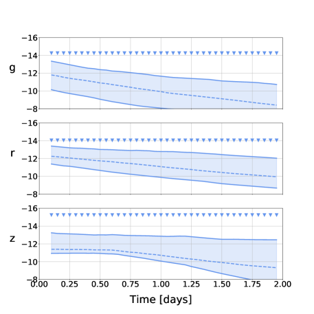
Figure 1: Variety of lightcurves consistent with the Dark Energy Camera based g/r/z limits on S190510g (Andreoni et al., 2019b), where we show median and 90% contours for lightcurves based on the Kasen et al. (2017) model.

Figure 1 gives an example of this approach for the candidate S190510g using the model of Kasen et al. (2017). It shows the upper limits derived from the Dark Energy Camera in horizontal lines for the three photometric bands $g$, $r$, and $z$. The absolute magnitudes correspond to the mean of the gravitational-wave distance. We also plot an example lightcurve consistent with these constraints. These include the uncertainty in distance sampling. Histograms of the ejecta masses (and other quantities) are made based on these lightcurves, creating the distributions derived in the following analyses.

3.2 Ejecta mass limits

Model I                                     Model II                                     Model III
S190425z

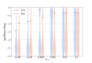
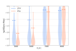
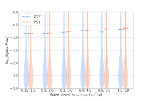
S190426c

S190510g

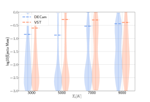
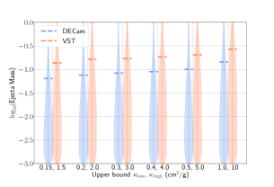
S190901ap

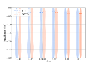
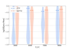
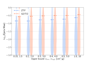
S190910h

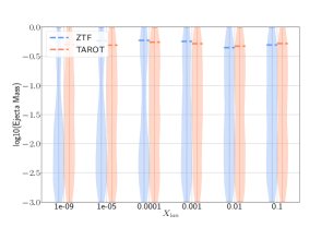
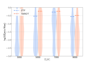
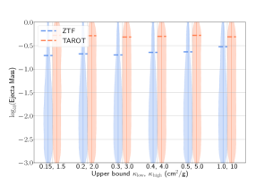
Figure 2: Probability density for the total ejecta mass for all considered events and all employed lightcurve models. From the top down, the events are S190425z, S190426c, S190510g, S190901ap, and S190910h. From the left to the right, we show constraints as a function of lanthanide fraction for based on the Kasen et al. (2017) model, as a function of temperature for the Bulla (2019) model with $\Phi=0^{\circ}$, and as a function of the opacity of the 2-components, $\kappa_{\rm low}$ and $\kappa_{\rm high}$. For S190425z, we use the ZTF (left, Kasliwal et al. (2019a)) and PS1 (right, Smith et al. (2019)) limits. For S190426c, we use the ZTF (Kasliwal et al., 2019b) and the DECam (Goldstein et al., 2019b) limits. For S190510g, we use DECam (Andreoni et al., 2019b) and VST (Grado et al., 2019a). For, S190901ap, we use the ZTF (Kool et al., 2019) and GOTO (Ackley et al., 2019b) observations. For S190910h, we use the ZTF (Stein et al., 2019a) and TAROT (Barynova et al., 2019b) observations.

In this section, we provide ejecta mass constraints from comparing different lightcurve models to observational upper limits for S190425z, S190426c, S190510g, S190901ap and S190910h. Specifically, we compute ejecta mass constraints for different values of one key quantity for each model: the lanthanide fraction (Model I), the temperature (Model II) and the opacities (Model III). Constraints on the ejecta mass are controlled by the impact of these three different parameters on the predicted kilonova brightness and color. Increasing the lanthanide fraction ($X_{\rm lan}$, Model I) and opacities ($\kappa_{\rm low}$ and $\kappa_{\rm high}$, Model III) shifts the escaping radiation to longer wavelengths and, thus, leads to the transition from a “blue” to a “red” kilonova. The impact of the temperature (Model II) on the brightness and color depends on the epoch since merger. However, at phases when data are most constraining ($\lesssim$ 2 d) an increase in temperature results in a shift of the emitted radiation from redder to bluer wavelengths. In particular, moving temperature from $3000$ to $9000$ K produces increasingly fainter kilonovae in both optical and near-infrared bands at these epochs.

Because of the different color predictions, telescopes observing in different regions of the spectrum are associated with different ejecta mass limits. For instance, optical telescopes are generally more constraining to “blue” kilonovae that have low lanthanide fractions.

S190425z: The top row of figure 2 shows the ejecta mass constraints for S190425z based on observations from ZTF (left, Kasliwal et al. (2019a)) and PS1 (right, Smith et al. (2019)). We mark the $90\%$ confidence with a horizontal dashed line. In general, the constraints on ejecta mass for the low lanthanide fractions are stronger than available for the “red kilonovae,” which are hidden in the redder photometric bands, cf. Model I. This is a result of using optical telescopes, which cover a large percentage of the sky localization, but are generally more constraining to “blue” kilonovae, i.e. those that have low lanthanide fractions. The $i$-band observations of PS1 lead to stronger constraints on the red side than is possible with ZTF for Model II, with similar constraints for Model I and Model III. With the higher intrinsic luminosities from Model II, the constraints in the redder bands from PS1 lead to notable improvements in the constraints. These constraints are not realized in Model I and Model III due to their lower intrinsic luminosities. We find that the different treatments of the heating rates and radiative transport, yield significantly different ejecta mass constraints than imposed by the effective opacity, temperature, and lanthanide fraction differences, i.e., differences between the three models are larger than within the individual models. Most notably, Model II produces, across all considered temperature ranges, the most stringent constraints. Consequently, while Model I and Model III only disfavor (in the most optimistic scenarios) ejecta masses $M_{\rm ej}\lesssim 0.1M_{\odot}$, which is very hard to achieve for a BNS merger, Model II places upper bounds on the ejecta mass of $M_{\rm ej}\lesssim 0.03M_{\odot}$ for temperatures at or below $5000K$.

S190426c: The second row of figure 2 shows the ejecta mass constraints for S190426c based on the observations from ZTF (Kasliwal et al., 2019b) and the DECam (Goldstein et al., 2019b). Despite the smaller sky area requiring coverage and therefore generally deeper exposures, the larger distance to this object leads to limits that are worse than for the first event. However, for a number of parameter combinations, we find that ejecta masses above $\sim 0.1M_{\odot}$ are ruled out based on the DECam observations. Furthermore, as for S190425z, one obtains tighter constraints for blue kilonova (low lanthanide fractions and opacities) for Model I and Model III, and for redder kilonovae in Model II.

S190510g: The third row of figure 2 shows the ejecta mass constraints for S190510g based on observations from DECam (Andreoni et al., 2019b) and VST (Grado et al., 2019a). The relative improvement of sensitivity between ZTF and DECam offsets the relative difference in distance estimates, yielding very similar ejecta mass constraints between the two binary neutron star coalescence candidates, i.e., S190510g and S190425z. The inclusion of the three bands, g-, r-, and z-band observations with DECam produces measurable constraints in both the blue and red bands; for example, with Model I, $M_{\rm ej}$ is $\lesssim 0.025M_{\odot}$ for the lowest lanthanide fractions.

S190901ap: The fourth row of figure 2 shows the ejecta mass constraints for S190901ap based on observations from ZTF (Kool et al., 2019) and GOTO (Ackley et al., 2019b). Due to the large sky localization covering more than 10,000 deg², there was relatively minimal EM follow-up investigation. The larger distance to this potential BHNS system results in the shallowest constraints on ejecta mass for all considered candidates.

S190910h: The final row of figure 2 shows the ejecta mass constraints for S190910h based on observations from ZTF (Stein et al., 2019a) and TAROT (Barynova et al., 2019b). Due to the large sky localization covering more than 20,000 deg², there was relatively minimal EM follow-up investigation, and therefore, similar to the event above, there were essentially no constraints.

Summary: Considering the five individual constraints, we find that S190425z and S190426c provide overall the tightest constraints for a BNS and BHNS candidate, respectively. However, our analysis shows that even for these events, no constraints can be obtained with Model III or for Model I in case for ejecta with high lanthanide fractions. These loose constraints are mainly caused by the large distance to the individual candidate events, which are generally several times further away than GW170817. Considering the results obtained from Model II, we will describe in the next section how potential ejecta mass constraints lead to constraints on the binary properties of BNS and BHNS candidates. However, we want to emphasize that there are large systematic differences between the lightcurve models and that the entire sky area provided by LIGO and Virgo has not been covered for all triggers. Thus, the following analysis should be rather interpreted as a proof of principle.

4 Constraining the binary parameters

Within this section, we present as a proof of principle possible constraints for the binary properties of the BNS candidate S190425z and the BHNS candidate S190426c (under the assumption that the source location was covered within the EM follow-up campaign). We focus on the results of Model II with a fixed temperature of $5000\rm K$. This leads to a maximum total ejecta masses of $0.03M_{\odot}$ for S190425z and $0.09M_{\odot}$ for S190426c.

4.1 The binary neutron star candidate S190425z

To ensure that the ejected material is massive enough to trigger a bright EM counterpart, the final remnant should not collapse promptly to a black hole (BH) after the merger. As mentioned in the introduction, prompt collapse formation depends dominantly on the total mass of the binary. As shown in Bauswein et al. (2013) the total mass of the binary $M$ has to be below a characteristic threshold mass:

$$M_{\rm thr}=\left(2.380-3.606\frac{M_{\rm TOV}}{R_{1.6M_{\odot}}}\right)M_{\rm TOV}$$ (1)

with $M_{\rm TOV}$ being the maximum supported mass for a spherical NS and $R_{1.6M_{\odot}}$ the radius of a $1.6M_{\odot}$ NS. Recently, the threshold mass estimate was updated by Köppel et al. (2019) incorporating a non-linear dependence on the maximum allowed compactness and Agathos et al. (2019) derived a prompt-collapse threshold estimate based on new numerical relativity simulations, mainly publicly available at http://www.computational-relativity.org (Dietrich et al., 2018). For our rough estimates presented here, we will use, for simplicity, the criterion given in Bauswein et al. (2013).

While for close GW events it would be a valid assumption that all configurations without an EM counterpart have masses above the prompt threshold mass, $M>M_{\rm thr}$, this assumption does not hold for systems with distances much larger than the one for GW170817, e.g., for S190425z. In general, the total ejecta mass, for which our previous analysis provided some upper limits, is related to the debris disk mass formed after the merger; here, we use the disk mass estimate presented in Coughlin et al. (2018a), where $M_{\rm disk}$ was a function on $M/M_{\rm thr}$:

$$\log_{10} \left(m_{\rm disk}\left[M_{\rm tot}/M_{\rm thr}\right]\right)=$$

$$\max\left(-3,\ a\left(1+b\tanh\left[\frac{c-M_{\rm tot}/M_{\rm thr}}{d}\right]\right)\right)$$ (2)

with the fitting parameters $a,b,c,d$; see Coughlin et al. (2018a). We emphasize that this estimate was based on a suite of numerical relativity simulations for equal-mass or near equal-mass systems, high mass ratio systems might lead to more massive disks Kiuchi et al. (2019) The mass of the disk wind is then $M_{\rm wind}=fM_{\rm disk}$ with the unknown conversion factor $f$. This efficiency parameter remains very uncertain (Fernández et al., 2015; Siegel & Metzger, 2018; Fernández et al., 2019; Christie et al., 2019) and we will vary it for our BNS analysis, $f\in[0.1,0.4].$ Since a fraction of the ejecta will also be released dynamically during the merger, not all of the total ejecta comes from disk winds. As an indication, we present the disk wind estimate in figure 3 assuming $100\%$ of the total ejecta mass for S190425z are connected to the wind ejecta (solid black line), $75\%$ of the total mass is assigned to winds (dashed line), and half of the total ejecta comes from disk wind ejecta (dotted line).

The two panels in figure 3 refer to different choices of the maximum TOV-mass $2.07M_{\odot}$ for the top and $2.30M_{\odot}$ for the bottom panel. These values are motivated by the recent observation of J0740+6620 (Cromartie et al., 2019) and the upper bound on the maximum mass following from GW170817, e.g. (Margalit & Metzger, 2017; Rezzolla et al., 2018; Shibata et al., 2019). In addition, we assume a radius $R_{1.6M_{\odot}}$ of $11.1\rm km$ in the top and $13.9\rm km$ in the bottom panel, as derived in Coughlin et al. (2018a).These combinations of $M_{\rm TOV}$ and $R_{1.6M_{\odot}}$ include the most extreme scenarios in terms of stiff and soft EOSs, and, thus, provide boundaries for our analysis. Considering the scenario for a very soft EOS, we find that the total mass of S190425z lies presumably above $2.40M_{\odot}$ if the efficiency factor if about $20\%$. Contrary for an efficiency factor of $20\%$ and a very stiff EOS, the total mass of S190425z would presumably be $2.9M\odot$.

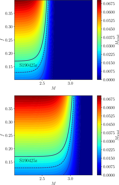
Figure 3: Disk wind ejecta as a function of the conversion factor $f$ and the total mass of the binary $M$. We include the upper bounds from S190425z using Model II for $5000\rm K$ assuming that the disk wind accounts for the entire ejecta mass (solid line), $75\%$ (dashed line) or for $50\%$ of the total ejecta (dotted line). The top panel assumes an EOS with a maximum TOV mass of $2.07M_{\odot}$ and a radius of $R_{1.6M_{\odot}}=11.1\rm km$, while the bottom panel uses $M_{\rm TOV}=2.30M_{\odot}$ and $R_{1.6M_{\odot}}=13.9\rm km$.

4.2 The black hole - neutron star candidate S190426c

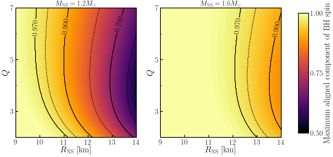
Figure 4: Maximum aligned component of the black hole spin as a function of neutron star radius and binary mass ratio for S190426c, if that event was a BHNS merger within the region covered by follow-up observations. We show results for $M_{\rm NS}=1.2M_{\odot}$ (left) and $M_{\rm NS}=1.6M_{\odot}$, and require $M_{\rm ej}<0.09M_{\odot}$ (Model II for $5000\rm K$). Dashes lines correspond to maximum spins of $0.6,0.8,0.95$, and solid lines to maximum spins of $0.7,0.9,0.97$. Only a small part of the parameter space (large aligned spin, low mass neutron stars) can possibly be ruled out be observations. The constraints for more massive stars ($M_{\rm NS}=1.6M_{\odot}$) are not reliable since the analytical models have not been tested for spins greater than $\sim 0.9$.

Similarly for BHNS systems, the absence of an observed kilonova constrains the initial parameters of the binary. As for the BNS case, the outflows from BHNS mergers can be divided into the dynamical ejecta, which is produced at the time of merger and typically lanthanide-rich (Deaton et al., 2013; Foucart et al., 2014; Kyutoku et al., 2018), and magnetically-driven or neutrino-driven disk winds produced in the $1-10$ seconds following the merger, which have a more uncertain composition (Fernández et al., 2015; Just et al., 2015; Siegel & Metzger, 2018; Fernández et al., 2019). The dynamical ejecta for neutron stars within the range of parameters used in numerical simulations so far is well modeled by the fit of Kawaguchi et al. (2016). Extrapolating that fit to more compact stars, however, leads to unphysical results (i.e. an increase in the ejected mass for more compact stars). Here, we use the modified formula

$$\frac{M_{\rm dyn}}{M^{b}_{\rm NS}}=\max\bigg{(}0,a_{1}Q^{n_{1}}(1-2C_{\rm NS})-a_{2}Q^{n_{2}}\frac{c^{2}R_{\rm ISCO}}{GM_{\rm BH}}+a_{3}\bigg{)}$$ (3)

with $Q=M_{\rm BH}/M_{\rm NS}$, $M^{b}_{\rm NS}$ the baryon mass of the neutron star, $C_{\rm NS}=GM_{\rm NS}/(R_{\rm NS}c^{2})$ its compactness, $R_{\rm ISCO}$ the radius of the innermost stable circular orbit around the black hole, and $a_{1}=0.007116,a_{2}=0.001436,a_{3}=-0.0276,n_{1}=0.8636,n_{2}=1.6840$ (see Krüger et al., in prep, for a more detailed discussion). Note that $R_{\rm ISCO}$ is computed for circular orbits around a black hole of dimensionless spin $\chi_{\rm eff}=\chi_{\parallel}$, with $\chi_{\parallel}$ the component of the black hole spin aligned with the orbital angular momentum of the binary. As a result, the ejected mass has a strong dependence in the aligned component of the black hole spin. The total mass in the bound accretion disk surrounding the remnant black hole can be estimated by subtracting $M_{\rm dyn}$ from the total amount of mass remaining outside of the black hole after merger $M_{\rm out}$. We compute $M_{\rm out}$ following the fit to numerical results provided in Foucart et al. (2018). Similarly to $M_{\rm dyn}$, $M_{\rm out}$ depends on the mass ratio of the system, the compactness of the neutron star, and the aligned component of the black hole spin. The mass in the disk winds is then $M_{\rm wind}=f(M_{\rm out}-M_{\rm dyn})$. Since the BHNS case contains already a larger number of free parameters, we fix the conversion factor to $f\gtrsim 0.15$ (Fernández et al., 2015; Siegel & Metzger, 2018; Fernández et al., 2019; Christie et al., 2019).

If S190426c was a BHNS merger within the region of the sky observed by ZTF and DECAM, and we assume the constraints obtained with Model II at $5000\rm K$, we argued that $M_{\rm ej}=M_{\rm dyn}+M_{\rm wind}$ has to be less than $0.09M_{\odot}$. Practically, this can be converted into a constrain excluding part of the 3-dimensional parameter space of $(Q,C_{\rm NS},\chi_{\parallel})$. Figure 4 visualizes this constraint as a maximum allowed value for the component of the dimensionless black hole spin aligned with the orbital angular momentum of the binary, as a function of neutron star size and binary mass ratio. We see that with this upper bound, the constraints on the parameter space of BHNS binaries are fairly weak: only large aligned black hole spins combined with low-mass stars and relatively stiff equations of state can possibly be ruled out.

5 Summary

We have presented an overview of the extensive searches for EM transients associated with a number of GW event triggers within the first half of the third observing run of Advanced LIGO and Advanced Virgo. Assuming that the individual sources were located in the covered sky region of the follow-up observations, we use three different kilonova models to derive possible upper limits on the ejecta mass compatible with the non-observation of EM signals for S190425z, S190426c, S190510g, S190901ap, and S190910h. Possibly informative constraints are obtained for S190425z and S190426c with the model of Bulla (2019). However, systematic uncertainties between different kilonova models are large and currently the dominating source of error in our analysis.

Based on our results, we computed potential lower limits on the total mass of S190425z from the non-existence of EM counterparts and find that it should have a total mass above $2.5M_{\odot}$ if we assume a soft and $2.9M_{\odot}$ if we assume a stiff EOS. Similarly, assuming that S190426c originated from a BHNS merger, we find that the non-observation of a kilonova could rule out large aligned black hole spins combined with low-mass stars (for stiff EOSs).

Our simple analysis shows that even without direct GW information, beyond the provided skymap and classification probability, source properties can be constrained. More importantly, inverting our approach, one sees that a fast estimation of the total mass can potentially be used to classify if potential GW candidates will cause bright EM counterparts. A similar approach has been recently outlined in Margalit & Metzger (2019).

In general, the limits derived on the ejecta mass for the events in the first six months of O3 are not striking, which shows that one should be striving to take deeper observations, perhaps at the cost of a smaller sky coverage. Assuming that AT2017gfo is representative, “interesting” limits are $\sim\,0.05\,M_{\odot}$, giving a ballpark limit to strive for. Those observations are most important at low latency, i.e., at times when kilonovae are brightest. In addition to adding and/or employing guiding to take longer observations, it might motivate the creation and use of stacking pipelines for survey facilities, for which this may be atypical.

Table 2: Reports of the observations by various teams of the sky localization area of gravitational-wave alerts of the possible BNS candidates S190425z, S190510g, S190901ap, S190910h and S190930t. Teams that employed “galaxy targeting” during their follow-up are not mentioned here. In the case where numbers were not reported or provided upon request, we recomputed some of them; if this was not possible, we add $-$.

Telescope	Filter	Limit mag	Delay aft. GW	Duration	GW sky localization area		reference
			(h)	(h)	name	coverage (%)
S190425z
ATLAS	o-band	$19.5$	$0.8$	$6.2$	bayestar ini	$37$	McBrien et al. (2019)
CNEOST	clear	$\approx 20$	$27.5$	$4.8$	bayestar ini	$10$	Xu et al. (2019b)
GOTO	L-band	$20.5$	$11.7$	$8.9$	bayestar ini	$30$	Steeghs et al. (2019a)
GRANDMA-TAROT	clear	$17.5$	$6.7$	$<63$	LALInference	$3$	Blazek et al. (2019a)
GROWTH-Gattini-IR	J-band	$15.5$	$1.0$	$27.8$	LALInference	$19$	De et al. (2019)
MASTER-network	clear	$\approx 18.5$	$\approx 0.0$	$144$	bayestar ini	$37$	Lipunov et al. (2019a)
Pan-STARRS	i-band	$21.5$	$1.3$	$<19$	bayestar ini	$28$	Smith et al. (2019)
SAGUARO	g-band	$\approx 21$	$1.3$	$1.3$	bayestar ini	$3$	Lundquist et al. (2019)
Xinglong-Schmidt	clear	$18$	$4.5$	$0.9$	bayestar ini	$3$	Xu et al. (2019a)
Zwicky Transient Facility	g/r-band	$\approx 21$	$1.0$	$27.8$	LALInference	$21$	Kasliwal et al. (2019a)
S190510g
ATLAS	o-band	$19.5$	$4.2$	$<12$	LALinference	4	Smartt et al. (2019a)
CNEOST	clear	$\approx 18.5$	$9.9$	$3.3$	bayestar ini	13	Li et al. (2019)
Dabancheng/HMT	clear	$\approx 18$	$13.0$	$6.0$	bayestar ini	$\approx 8$	Xu et al. (2019d)
GRAWITA-VST	r-sloan	$22$	$21.1$	$<6$	LALInference	$50$	Grado et al. (2019a)
GROWTH-DECAM	g/r/z-band	$21.7/22.3/21.2$	$3.0$	$18.5$	LALInference	$65$	Andreoni et al. (2019b)
HSC	Y-band	$22.7$	$<6$	$<12$	bayestar ini	$12$	Yoshida et al. (2019)
KMTNet	R-band	$21.7$	$13.6$	$<12$	LALInference	$66$	Im et al. (2019)
MASTER-network	clear	$\approx 18.5$	$\approx 0$	144	bayestar ini	$52$	Lipunov et al. (2019c)
Pan-STARRS	w/i-band	$20.5$	$4.2$	$<12$	LALInference	4	Smartt et al. (2019a)
Xinglong-Schmidt	clear	$18.5$	$9.8$	$5.8$	bayestar ini	$19$	Zhu et al. (2019)
DECAM-KMTNet	r-R band	$>22$	$3.0$	$<24$	LALInference	$69$	-
CNEOST-HMT-MASTER-Xinglong-TAROT	clear	$>18$	$1.0$	$<24$	LALInference	$71$	-
S190901ap
GOTO	L-band	$20$	$0.1$	$54$	bayestar ini	$28$	Ackley et al. (2019b)
GRANDMA-TAROT	clear	$17.5$	$0.4$	$<58.6$	LALInference	$9$	Barynova et al. (2019a)
MASTER-network	clear	$\approx 18.5$	$5.5$	168	bayestar ini	$32$	Lipunov et al. (2019e)
SVOM-GWAC	R-band	$16.3$	12.0	9	bayestar ini	$16$	Wei et al. (2019)
Zwicky Transient Facility	g/r-band	$20.7/20.7$	$3.6$	$\sim 72$	LALInference	$73$	Kool et al. (2019)
S190910h
GRANDMA-TAROT	clear	$18$	$10.5$	$<129$	LALInference	$1$	Barynova et al. (2019b)
MASTER-network	clear	$\approx 18.5$	$2.6$	144	bayestar ini	$8$	Lipunov et al. (2019g)
Zwicky Transient Facility	g/r-band	$20.7/20.7$	$1.80$	$1.5$	bayestar ini	34	Stein et al. (2019a)
S190930t
ATLAS	o-band	$19.5$	$0.0$	$144$	bayestar ini	$19$	Smartt et al. (2019b)
MASTER-network	clear	$\approx 18.5$	$\approx 0$	72	bayestar ini	$10$	Lipunov et al. (2019g)
Zwicky Transient Facility	g/r-band	$20.4/20.4$	$11.9$	$10.0$	bayestar ini	$45$	Stein et al. (2019b)

Table 3: Reports of the observations by various teams of the sky localization area of gravitational-wave alerts of possible BHNS candidates S190426c, S190814bv, S190910d and S190923y. Teams that employed “galaxy targeting” during their follow-up are not mentioned here. In the case where numbers were not reported or provided upon request, we recomputed some of them; if this was not possible, we add $-$.

Telescope	Filter	Limit mag	Delay aft. GW	Duration	GW sky localization area		reference
			(h)	(h)	name	coverage (%)
S190426c
ASAS-SN	g-band	$\approx 18$	-	$\approx 24$	bayestar ini	$86$	Shappee et al. (2019)
CNEOST	clear	$\approx 20$	$1.3$	$3.5$	bayestar ini	$35$	Xu et al. (2019c)
DDOTI/OAN	w-band	$\approx 18.5$	$14.7$	$4.9$	bayestar ini	$\approx 37$	Watson et al. (2019)
GOTO	g-band	$19.9$	$5.3$	$8.9$	LALInference	$54$	Steeghs et al. (2019b)
GRANDMA-OAJ	r-band	$19.6$	$6.3$	$4.9$	bayestar ini	$11$	Blazek et al. (2019b)
GRAWITA-Asiago	r-band	$\approx 16$	$6.9$	$0.5$	LALInference	$2$	Melandri et al. (2019)
GROWTH-DECAM	r/z-band	$22.9/22.5$	$7.6$	$11.5$	LALInference	$8.0$	Goldstein et al. (2019a)
GROWTH-Gattini-IR	J-band	$\approx 14.5$	$11.8$	$9.8$	bayestar ini	$92$	Hankins et al. (2019a)
GROWTH-INDIA	r-band	$20.5$	$2.0$	$29.4$	bayestar ini	$4$	Bhalerao et al. (2019)
J-GEM	clear	$20$	$19$	-	bayestar ini	-	Niino et al. (2019)
MASTER-network	clear	$\approx 18.5$	$\approx 0$	$144$	bayestar ini	$53$	Lipunov et al. (2019b)
SAGUARO	g-band	$\approx 21$	41.8	$\approx 24$	bayestar ini	$5$	Lundquist et al. (2019)
Zwicky Transient Facility	g/r-band	$\approx 21$	$13.0$	$31.3$	bayestar ini	$75$	Kasliwal et al. (2019b)
S190814bv
ATLAS	o-band	$>16$	$<12$	$24.0$	LALinference	$99$	Srivastav et al. (2019)
DESGW-DECam	r/i-band	$23.4,22.6$	$9.5$	$\approx 96$	LALInference	$90$	Soares-Santos et al. (2019)
DDOTI/OAN	w-band	$\approx 18.5$	$10.8$	$3.9$	LALInference	$90$	Dichiara et al. (2019)
GOTO	L-band	$18.4$	$3.5$	$5.0$	LALInference	$83$	Ackley et al. (2019a)
GRAWITA-VST	r-sloan	$\approx 22$	$11.7$	$1.3$	LALInference	$65$	Grado et al. (2019b)
GROWTH-Gattini-IR	J-band	$\approx 17.0$	$8.9$	$96.0$	bayestar ini	$90$	Hankins et al. (2019b)
KMTNet	R-band	$22.0$	$8.4$	$<12$	LALinference	$98$	Kim et al. (2019)
MASTER-network	clear	$\approx 18$	$0.4$	$6.7$	bayestar ini	$98$	Lipunov et al. (2019d)
MeerLICHT	u/q/i-band	$18.5/19.7/19.1$	$2.0$	$5.1$	bayestar HLV	$95$	Groot et al. (2019)
Pan-STARRS	i/z-band	$20.8/20.3$	$15.5$	$2.55$	LALInference	89	Smartt et al. (2019a)
Swope	r-band	$\approx 20.0$	$6.3$	$5.1$	LALinference	$42$	Kilpatrick et al. (2019)
GRANDMA-TCA	clear	$18.0$	$3.0$	$2.5$	bayestar HLV	$27$	Klotz et al. (2019)
GRANDMA-TRE	clear	$17.0$	$0.5$	$1.0$	LALinference	$76$	Christensen et al. (2019)
Zwicky Transient Facility	g/r/i-band	$20.3$	$13.3$	$1.7$	bayestar ini HLV	$86$	Singer et al. (2019)
MASTER-TAROT	clear	$>17$	$0.5$	$<3$	LALInference	$89$	-
S190910d
DDOTI/OAN	w-band	$\approx 18.5$	$3.0$	$4.7$	LALInference	$5$	Pereyra et al. (2019)
GRANDMA-TAROT	clear	$\approx 17.5$	$1.0$	$<67$	LALInference	$37$	Noysena et al. (2019)
MASTER-network	clear	$\approx 18.5$	$\approx 0$	$144$	bayestar ini	$25$	Lipunov et al. (2019f)
Zwicky Transient Facility	g/r-band	$20.8$	$1.5$	$1.5$	bayestar ini	$34$	Anand et al. (2019)
S190923y
GRANDMA-TAROT	clear	$\approx 17.5$	$3.7$	$<56.1$	bayestar ini	$26$	Turpin et al. (2019)
MASTER-network	clear	$\approx 18.5$	$\approx 0$	$144$	bayestar ini	$58$	Lipunov et al. (2019h)

References

- Abbott B. P. (2017) Abbott B. P. e. a., 2017, Phys. Rev. Lett., 119, 161101
- Abbott B.P. (2019) Abbott B.P. e. a., 2019, ] 10.3847/1538-4357/ab0e8f, 875, 161
- Abbott et al. (2017a) Abbott et al. 2017a, Nature, 551, 85
- Abbott et al. (2017b) Abbott B. P., et al., 2017b, Astrophys. J., 848, L12
- Abbott et al. (2017c) Abbott B. P., et al., 2017c, The Astrophysical Journal Letters, 848, L13
- Ackley et al. (2019a) Ackley K., et al., 2019a, GRB Coordinates Network, 25337
- Ackley et al. (2019b) Ackley K., et al., 2019b, GRB Coordinates Network, 25654
- Agathos et al. (2019) Agathos M., Zappa F., Bernuzzi S., Perego A., Breschi M., Radice D., 2019
- Anand et al. (2019) Anand S., et al., 2019, GRB Coordinates Network, 25706
- Andreoni et al. (2019a) Andreoni I., et al., 2019a
- Andreoni et al. (2019b) Andreoni I., et al., 2019b, Astrophys. J., 881, L16
- Arcavi et al. (2017) Arcavi et al. 2017, Nature, 551, 64 EP
- Arnett (1982) Arnett W. D., 1982, ApJ, 253, 785
- Baker et al. (2017) Baker T., Bellini E., Ferreira P. G., Lagos M., Noller J., Sawicki I., 2017, Phys. Rev. Lett., 119, 251301
- Barynova et al. (2019a) Barynova K., et al., 2019a, GRB Coordinates Network, 25666
- Barynova et al. (2019b) Barynova K., et al., 2019b, GRB Coordinates Network, 25780
- Bauswein et al. (2013) Bauswein A., Baumgarte T. W., Janka H. T., 2013, Phys. Rev. Lett., 111, 131101
- Bauswein et al. (2017) Bauswein A., et al., 2017, The Astrophysical Journal Letters, 850, L34
- Bellm et al. (2018) Bellm E. C., et al., 2018, Publications of the Astronomical Society of the Pacific, 131, 018002
- Bhalerao et al. (2019) Bhalerao V., et al., 2019, GRB Coordinates Network, 24258
- Blazek et al. (2019a) Blazek M., et al., 2019a, GRB Coordinates Network, 24227
- Blazek et al. (2019b) Blazek M., et al., 2019b, GRB Coordinates Network, 24327
- Bulla (2019) Bulla M., 2019, MNRAS, 489, 5037
- Capano et al. (2019) Capano C. D., et al., 2019
- Christensen et al. (2019) Christensen N., et al., 2019, GRB Coordinates Network, 25599
- Christie et al. (2019) Christie I. M., Lalakos A., Tchekhovskoy A., Fernández R., Foucart F., Quataert E., Kasen D., 2019
- Cook et al. (2019) Cook D. O., et al., 2019, GRB Coordinates Network, 24232
- Coughlin et al. (2017) Coughlin M., Dietrich T., Kawaguchi K., Smartt S., Stubbs C., Ujevic M., 2017, ApJ, 849, 12
- Coughlin et al. (2018a) Coughlin M. W., Dietrich T., Margalit B., Metzger B. D., 2018a, arXiv e-prints,
- Coughlin et al. (2018b) Coughlin M. W., et al., 2018b, Monthly Notices of the Royal Astronomical Society, 480, 3871
- Coughlin et al. (2019a) Coughlin M. W., Dietrich T., Heinzel J., Khetan N., Antier S., Christensen N., Coulter D. A., Foley R. J., 2019a
- Coughlin et al. (2019b) Coughlin M. W., et al., 2019b, arXiv e-prints, p. arXiv:1907.12645
- Coulter et al. (2017) Coulter D. A., et al., 2017, Science, 358, 1556
- Creminelli & Vernizzi (2017) Creminelli P., Vernizzi F., 2017, Phys. Rev. Lett., 119, 251302
- Cromartie et al. (2019) Cromartie H. T., et al., 2019
- Dado & Dar (2019) Dado S., Dar A., 2019
- De et al. (2019) De K., et al., 2019, GRB Coordinates Network, 24187
- Deaton et al. (2013) Deaton M. B., et al., 2013, Astrophys. J., 776, 47
- Dekany et al. (2019) Dekany Smith et al., 2019, Submitted to PASP
- Dhawan et al. (2019) Dhawan S., Bulla M., Goobar A., Sagués Carracedo A., Setzer C. N., 2019, arXiv e-prints, p. arXiv:1909.13810
- Dichiara et al. (2019) Dichiara S., et al., 2019, GRB Coordinates Network, 25352
- Dietrich & Ujevic (2017) Dietrich T., Ujevic M., 2017, Class. Quant. Grav., 34, 105014
- Dietrich et al. (2018) Dietrich T., et al., 2018, Class. Quant. Grav., 35, 24LT01
- Doctor et al. (2017) Doctor Z., Farr B., Holz D. E., Pürrer M., 2017, preprint, (arXiv:1706.05408)
- Eichler et al. (1989) Eichler D., Livio M., Piran T., Schramm D. N., 1989, Nature, 340, 126
- Etienne et al. (2009) Etienne Z. B., Liu Y. T., Shapiro S. L., Baumgarte T. W., 2009, Phys. Rev., D79, 044024
- Ezquiaga & Zumalacárregui (2017) Ezquiaga J. M., Zumalacárregui M., 2017, Phys. Rev. Lett., 119, 251304
- Fernández et al. (2015) Fernández R., Kasen D., Metzger B. D., Quataert E., 2015, Mon. Not. Roy. Astron. Soc., 446, 750
- Fernández et al. (2019) Fernández R., Tchekhovskoy A., Quataert E., Foucart F., Kasen D., 2019, Mon. Not. Roy. Astron. Soc., 482, 3373
- Foucart (2012) Foucart F., 2012, Phys. Rev., D86, 124007
- Foucart et al. (2014) Foucart F., et al., 2014, Phys. Rev., D90, 024026
- Foucart et al. (2018) Foucart F., Hinderer T., Nissanke S., 2018, Phys. Rev., D98, 081501
- Goldstein et al. (2019a) Goldstein D. A., et al., 2019a, Astrophys. J., 881, L7
- Goldstein et al. (2019b) Goldstein D. A., et al., 2019b, GRB Coordinates Network, 24257
- Grado et al. (2019a) Grado A., et al., 2019a, GRB Coordinates Network, 24484
- Grado et al. (2019b) Grado A., et al., 2019b, GRB Coordinates Network, 25371
- Graham et al. (2019) Graham M. J., et al., 2019, Publications of the Astronomical Society of the Pacific, 131, 078001
- Groot et al. (2019) Groot P., et al., 2019, GRB Coordinates Network, 25340
- Hankins et al. (2019a) Hankins M., et al., 2019a, GRB Coordinates Network, 24284
- Hankins et al. (2019b) Hankins M., et al., 2019b, GRB Coordinates Network, 25358
- Hotokezaka & Nakar (2019) Hotokezaka K., Nakar E., 2019
- Hotokezaka et al. (2013) Hotokezaka K., Kiuchi K., Kyutoku K., Okawa H., Sekiguchi Y.-i., Shibata M., Taniguchi K., 2013, Phys. Rev., D87, 024001
- Hotokezaka et al. (2019) Hotokezaka K., Nakar E., Gottlieb O., Nissanke S., Masuda K., Hallinan G., Mooley K. P., Deller A., 2019, Nature Astron.
- Im et al. (2019) Im M., et al., 2019, GRB Coordinates Network, 24466
- Just et al. (2015) Just O., Bauswein A., Pulpillo R. A., Goriely S., Janka H. T., 2015, Mon. Not. Roy. Astron. Soc., 448, 541
- Kapadia et al. (2019) Kapadia S. J., et al., 2019
- Kasen et al. (2017) Kasen D., Metzger B., Barnes J., Quataert E., Ramirez-Ruiz E., 2017, Nature, 551, 80 EP
- Kasliwal et al. (2019a) Kasliwal M. M., et al., 2019a, GRB Coordinates Network, 24191
- Kasliwal et al. (2019b) Kasliwal M. M., et al., 2019b, GRB Coordinates Network, 24283
- Kawaguchi et al. (2016) Kawaguchi K., Kyutoku K., Shibata M., Tanaka M., 2016, Astrophys. J., 825, 52
- Kilpatrick et al. (2019) Kilpatrick C., et al., 2019, GRB Coordinates Network, 25350
- Kim et al. (2019) Kim J., et al., 2019, GRB Coordinates Network, 25342
- Kiuchi et al. (2019) Kiuchi K., Kyutoku K., Shibata M., Taniguchi K., 2019, Astrophys. J., 876, L31
- Klotz et al. (2019) Klotz A., et al., 2019, GRB Coordinates Network, 25338
- Kool et al. (2019) Kool E., et al., 2019, GRB Coordinates Network, 25616
- Köppel et al. (2019) Köppel S., Bovard L., Rezzolla L., 2019, Astrophys. J., 872, L16
- Korobkin et al. (2012) Korobkin O., Rosswog S., Arcones A., Winteler C., 2012, Monthly Notices of the Royal Astronomical Society, 426, 1940
- Kyutoku et al. (2015) Kyutoku K., Ioka K., Okawa H., Shibata M., Taniguchi K., 2015, Phys. Rev., D92, 044028
- Kyutoku et al. (2018) Kyutoku K., Kiuchi K., Sekiguchi Y., Shibata M., Taniguchi K., 2018, Phys. Rev., D97, 023009
- LIGO Scientific Collaboration & Virgo Collaboration (2019a) LIGO Scientific Collaboration Virgo Collaboration 2019a, GRB Coordinates Network, 24168
- LIGO Scientific Collaboration & Virgo Collaboration (2019b) LIGO Scientific Collaboration Virgo Collaboration 2019b, GRB Coordinates Network, 24228
- LIGO Scientific Collaboration & Virgo Collaboration (2019c) LIGO Scientific Collaboration Virgo Collaboration 2019c, GRB Coordinates Network, 24237
- LIGO Scientific Collaboration & Virgo Collaboration (2019d) LIGO Scientific Collaboration Virgo Collaboration 2019d, GRB Coordinates Network, 24279
- LIGO Scientific Collaboration & Virgo Collaboration (2019e) LIGO Scientific Collaboration Virgo Collaboration 2019e, GRB Coordinates Network, 24411
- LIGO Scientific Collaboration & Virgo Collaboration (2019f) LIGO Scientific Collaboration Virgo Collaboration 2019f, GRB Coordinates Network, 24442
- LIGO Scientific Collaboration & Virgo Collaboration (2019g) LIGO Scientific Collaboration Virgo Collaboration 2019g, GRB Coordinates Network, 24448
- LIGO Scientific Collaboration & Virgo Collaboration (2019h) LIGO Scientific Collaboration Virgo Collaboration 2019h, GRB Coordinates Network, 24489
- LIGO Scientific Collaboration & Virgo Collaboration (2019i) LIGO Scientific Collaboration Virgo Collaboration 2019i, GRB Coordinates Network, 24591
- LIGO Scientific Collaboration & Virgo Collaboration (2019j) LIGO Scientific Collaboration Virgo Collaboration 2019j, GRB Coordinates Network, 24656
- LIGO Scientific Collaboration & Virgo Collaboration (2019k) LIGO Scientific Collaboration Virgo Collaboration 2019k, GRB Coordinates Network, 25087
- LIGO Scientific Collaboration & Virgo Collaboration (2019l) LIGO Scientific Collaboration Virgo Collaboration 2019l, GRB Coordinates Network, 25187
- LIGO Scientific Collaboration & Virgo Collaboration (2019m) LIGO Scientific Collaboration Virgo Collaboration 2019m, GRB Coordinates Network, 25208
- LIGO Scientific Collaboration & Virgo Collaboration (2019n) LIGO Scientific Collaboration Virgo Collaboration 2019n, GRB Coordinates Network, 25296
- LIGO Scientific Collaboration & Virgo Collaboration (2019o) LIGO Scientific Collaboration Virgo Collaboration 2019o, GRB Coordinates Network, 25324
- LIGO Scientific Collaboration & Virgo Collaboration (2019p) LIGO Scientific Collaboration Virgo Collaboration 2019p, GRB Coordinates Network, 25333
- LIGO Scientific Collaboration & Virgo Collaboration (2019q) LIGO Scientific Collaboration Virgo Collaboration 2019q, GRB Coordinates Network, 25367
- LIGO Scientific Collaboration & Virgo Collaboration (2019r) LIGO Scientific Collaboration Virgo Collaboration 2019r, GRB Coordinates Network, 25442
- LIGO Scientific Collaboration & Virgo Collaboration (2019s) LIGO Scientific Collaboration Virgo Collaboration 2019s, GRB Coordinates Network, 25549
- LIGO Scientific Collaboration & Virgo Collaboration (2019t) LIGO Scientific Collaboration Virgo Collaboration 2019t, GRB Coordinates Network, 25606
- LIGO Scientific Collaboration & Virgo Collaboration (2019u) LIGO Scientific Collaboration Virgo Collaboration 2019u, GRB Coordinates Network, 25614
- LIGO Scientific Collaboration & Virgo Collaboration (2019v) LIGO Scientific Collaboration Virgo Collaboration 2019v, GRB Coordinates Network, 25695
- LIGO Scientific Collaboration & Virgo Collaboration (2019w) LIGO Scientific Collaboration Virgo Collaboration 2019w, GRB Coordinates Network, 25707
- LIGO Scientific Collaboration & Virgo Collaboration (2019x) LIGO Scientific Collaboration Virgo Collaboration 2019x, GRB Coordinates Network, 25723
- LIGO Scientific Collaboration & Virgo Collaboration (2019y) LIGO Scientific Collaboration Virgo Collaboration 2019y, GRB Coordinates Network, 25778
- LIGO Scientific Collaboration & Virgo Collaboration (2019z) LIGO Scientific Collaboration Virgo Collaboration 2019z, GRB Coordinates Network, 25814
- LIGO-Virgo collaboration (2019) LIGO-Virgo collaboration 2019, GRB Coordinates Network, 25876
- Lattimer & Schramm (1974) Lattimer J. M., Schramm D. N., 1974, ApJ, 192, L145
- Lattimer & Schramm (1976) Lattimer J. M., Schramm D. N., 1976, ApJ, 210, 549
- Lee & Ramirez-Ruiz (2007) Lee W. H., Ramirez-Ruiz E., 2007, New Journal of Physics, 9, 17
- Li & Paczynski (1998) Li L.-X., Paczynski B., 1998, The Astrophysical Journal Letters, 507, L59
- Li et al. (2019) Li B., et al., 2019, GRB Coordinates Network, 24465
- Lipunov et al. (2017) Lipunov V., et al., 2017, The Astrophysical Journal Letters, 850, L1
- Lipunov et al. (2019a) Lipunov V., et al., 2019a, GRB Coordinates Network, 24167
- Lipunov et al. (2019b) Lipunov V., et al., 2019b, GRB Coordinates Network, 24236
- Lipunov et al. (2019c) Lipunov V., et al., 2019c, GRB Coordinates Network, 24436
- Lipunov et al. (2019d) Lipunov V., et al., 2019d, GRB Coordinates Network, 25322
- Lipunov et al. (2019e) Lipunov V., et al., 2019e, GRB Coordinates Network, 25609
- Lipunov et al. (2019f) Lipunov V., et al., 2019f, GRB Coordinates Network, 25694
- Lipunov et al. (2019g) Lipunov V., et al., 2019g, GRB Coordinates Network, 25712
- Lipunov et al. (2019h) Lipunov V., et al., 2019h, GRB Coordinates Network, 25812
- Lundquist et al. (2019) Lundquist M. J., et al., 2019, arXiv e-prints, p. arXiv:1906.06345
- Margalit & Metzger (2017) Margalit B., Metzger B. D., 2017, Astrophys. J., 850, L19
- Margalit & Metzger (2019) Margalit B., Metzger B. D., 2019
- Masci et al. (2018) Masci F. J., et al., 2018, Publications of the Astronomical Society of the Pacific, 131, 018003
- McBrien et al. (2019) McBrien O., et al., 2019, GRB Coordinates Network, 24197
- Melandri et al. (2019) Melandri A., et al., 2019, GRB Coordinates Network, 24340
- Metzger et al. (2010) Metzger B. D., et al., 2010, Monthly Notices of the Royal Astronomical Society, 406, 2650
- Mochkovitch et al. (1993) Mochkovitch R., Hernanz M., Isern J., Martin X., 1993, Nature, 361, 236
- Mooley et al. (2017) Mooley K. P., et al., 2017, Nature, 554, 207 EP
- Nakar (2007) Nakar E., 2007, Phys. Rept., 442, 166
- Narayan et al. (1992) Narayan R., Paczynski B., Piran T., 1992, ApJ, 395, L83
- Niino et al. (2019) Niino Y., et al., 2019, GRB Coordinates Network, 24299
- Noysena et al. (2019) Noysena K., et al., 2019, GRB Coordinates Network, 25749
- Paczynski (1991) Paczynski B., 1991, Acta Astron., 41, 257
- Pannarale et al. (2011) Pannarale F., Tonita A., Rezzolla L., 2011, Astrophys. J., 727, 95
- Pedregosa et al. (2011) Pedregosa F., et al., 2011, Journal of Machine Learning Research, 12, 2825
- Pereyra et al. (2019) Pereyra E., et al., 2019, GRB Coordinates Network, 25737
- Radice & Dai (2019) Radice D., Dai L., 2019, Eur. Phys. J., A55, 50
- Radice et al. (2018) Radice D., Perego A., Zappa F., Bernuzzi S., 2018, The Astrophysical Journal Letters, 852, L29
- Rasmussen & Williams (2006) Rasmussen C. E., Williams C. K. I., 2006, Gaussian Processes for Machine Learning. MIT Press
- Rezzolla et al. (2018) Rezzolla L., Most E. R., Weih L. R., 2018, Astrophys. J., 852, L25
- Roberts et al. (2011) Roberts L. F., Kasen D., Lee W. H., Ramirez-Ruiz E., 2011, The Astrophysical Journal Letters, 736, L21
- Sakstein & Jain (2017) Sakstein J., Jain B., 2017, Phys. Rev. Lett., 119, 251303
- Sari et al. (1998) Sari R., Piran T., Narayan R., 1998, ApJ, 497, L17
- Savchenko et al. (2017) Savchenko V., et al., 2017, The Astrophysical Journal, 848, L15
- Shappee et al. (2019) Shappee B., et al., 2019, GRB Coordinates Network, 24309
- Shibata et al. (2019) Shibata M., Zhou E., Kiuchi K., Fujibayashi S., 2019
- Siegel & Metzger (2018) Siegel D. M., Metzger B. D., 2018, Astrophys. J., 858, 52
- Singer et al. (2019) Singer et al. 2019, GRB Coordinates Network, 25343
- Smartt et al. (2019a) Smartt S., et al., 2019a, GRB Coordinates Network, 24517
- Smartt et al. (2019b) Smartt S., et al., 2019b, GRB Coordinates Network, 25922
- Smith et al. (2019) Smith K. W., et al., 2019, GRB Coordinates Network, 24210
- Soares-Santos et al. (2017) Soares-Santos et al. 2017, The Astrophysical Journal Letters, 848, L16
- Soares-Santos et al. (2019) Soares-Santos M., et al., 2019, GRB Coordinates Network, 25336
- Srivastav et al. (2019) Srivastav S., et al., 2019, GRB Coordinates Network, 25375
- Steeghs et al. (2019a) Steeghs D., et al., 2019a, GRB Coordinates Network, 24224
- Steeghs et al. (2019b) Steeghs D., et al., 2019b, GRB Coordinates Network, 24291
- Stein et al. (2019a) Stein R., et al., 2019a, GRB Coordinates Network, 25722
- Stein et al. (2019b) Stein R., et al., 2019b, GRB Coordinates Network, 25899
- Tanvir et al. (2013) Tanvir N. R., Levan A. J., Fruchter A. S., Hjorth J., Hounsell R. A., Wiersema K., Tunnicliffe R. L., 2013, Nature, 500, 547 EP
- Troja et al. (2017) Troja E., et al., 2017, Nature, 551, 71 EP
- Turpin et al. (2019) Turpin D., et al., 2019, GRB Coordinates Network, 25847
- Valenti et al. (2017) Valenti et al. 2017, The Astrophysical Journal Letters, 848, L24
- Veitch et al. (2015) Veitch J., et al., 2015, Phys. Rev. D, 91, 042003
- Watson et al. (2019) Watson A. M., et al., 2019, GRB Coordinates Network, 24310
- Wei et al. (2019) Wei J., et al., 2019, GRB Coordinates Network, 25648
- Xu et al. (2019a) Xu D., et al., 2019a, GRB Coordinates Network, 24190
- Xu et al. (2019b) Xu D., et al., 2019b, GRB Coordinates Network, 24285
- Xu et al. (2019c) Xu D., et al., 2019c, GRB Coordinates Network, 24286
- Xu et al. (2019d) Xu D., et al., 2019d, GRB Coordinates Network, 24476
- Yoshida et al. (2019) Yoshida M., et al., 2019, GRB Coordinates Network, 24450
- Zhu et al. (2019) Zhu Z., et al., 2019, GRB Coordinates Network, 24475