Katyusha Acceleration for Convex Finite-Sum Compositional Optimization

Abstract

Structured optimization problems arise in many applications. To efficiently solve these problems, it is important to leverage the structure information in the algorithmic design. This paper focuses on convex problems with a finite-sum compositional structure. Finite-sum problems appear as the sample average approximation of a stochastic optimization problem and also arise in machine learning with a huge amount of training data. One popularly used numerical approach for finite-sum problems is the stochastic gradient method (SGM). However, the additional compositional structure prohibits easy access to unbiased stochastic approximation of the gradient, so directly applying the SGM to a finite-sum compositional optimization problem (COP) is often inefficient.

We design new algorithms for solving strongly-convex and also convex two-level finite-sum COPs. Our design incorporates the Katyusha acceleration technique and adopts the mini-batch sampling from both outer-level and inner-level finite-sum. We first analyze the algorithm for strongly-convex finite-sum COPs. Similar to a few existing works, we obtain linear convergence rate in terms of the expected objective error, and from the convergence rate result, we then establish complexity results of the algorithm to produce an $\varepsilon$-solution. Our complexity results have the same dependence on the number of component functions as existing works. However, due to the use of Katyusha acceleration, our results have better dependence on the condition number $\kappa$ and improve to $\kappa^{2.5}$ from the best-known $\kappa^{3}$. Finally, we analyze the algorithm for convex finite-sum COPs, which uses as a subroutine the algorithm for strongly-convex finite-sum COPs. Again, we obtain better complexity results than existing works in terms of the dependence on $\varepsilon$, improving to $\varepsilon^{-2.5}$ from the best-known $\varepsilon^{-3}$.

1 Introduction

Utilizing structure information of a problem is crucial for designing efficient algorithms, especially when the problem involves a high-dimensional variable and/or a huge amount of data. For example, recent works (e.g., johnson2013accelerating ; xiao2014proximal ) have shown that on solving a finite-sum problem, the variance-reduced stochastic gradient method, which utilizes the finite-sum structure information, can significantly outperform a deterministic gradient method and a non-variance-reduced stochastic gradient method.

In this paper, we focus on the finite-sum compositional optimization problem (COP):

$$\min_{x\in\mathbb{R}^{N_{2}}}H(x)\equiv\frac{1}{n_{1}}\sum_{i=1}^{n_{1}}F_{i}\left(\frac{1}{n_{2}}\sum_{j=1}^{n_{2}}G_{j}(x)\right)+h(x),$$ (1.1)

where $F_{i}\colon\mathbb{R}^{N_{1}}\rightarrow\mathbb{R}$ is a differentiable function for each $i=1,\ldots,n_{1}$, $G_{j}\colon\mathbb{R}^{N_{2}}\rightarrow\mathbb{R}^{N_{1}}$ is a differentiable map for each $j=1,\ldots,n_{2}$, and $h$ is a simple (but possibly non-differentiable) function. For ease of description, we let $F\colon\mathbb{R}^{N_{1}}\rightarrow\mathbb{R}$ and $G\colon\mathbb{R}^{N_{2}}\rightarrow\mathbb{R}^{N_{1}}$ respectively denote the average of $\{F_{i}\}$ and $\{G_{j}\}$, i.e.,

$$F=\frac{1}{n_{1}}\sum_{i=1}^{n_{1}}F_{i},\quad G=\frac{1}{n_{2}}\sum_{j=1}^{n_{2}}G_{j}.$$

Also, we let $f\colon\mathbb{R}^{N_{2}}\rightarrow\mathbb{R}$ be the composition of $F$ with $G$, namely,

$$f=F\circ G.$$ (1.2)

The problem (1.1) can be viewed as a sample average approximation (SAA) of a two-level stochastic COP, for which wang2017stochastic propose and analyze a class of stochastic compositional gradient methods. Very recently, yang2019multilevel ; zhang2019multi extend the results to a multiple-level stochastic COP. Although it is possible to extend our method and analysis to a multiple-level finite-sum COP, we will focus on the two-level case because of the applications that we are interested in. Our main goal is to design a gradient-based (also called first-order) algorithm for (1.1) and to analyze its complexity to produce a stochastic $\varepsilon$-solution $\bar{x}$, i.e., ${\mathbb{E}}\big{[}H(\bar{x})-H(x^{\ast})\big{]}\leq\varepsilon$, where $x^{\ast}$ is a minimizer of $H$. The complexity is measured by the number of gradient evaluations of each $F_{i}$ and Jacobian matrix evaluations of each $G_{j}$. The method in wang2017stochastic can certainly be applied to (1.1). However, due to the utilization of the finite-sum structure, our method can have significantly better complexity result.

Below, we give two examples that motivate us to consider problems in the form of (1.1).

Example I: Risk-Averse Learning. Given a set of data $\{(\boldsymbol{a}_{i},b_{i})\}_{i=1}^{n}$ sampled from a certain distribution, the (sample) mean-variance minimization MR3235228 ; MR1094565 can be formulated as

$$\displaystyle\min_{\boldsymbol{x}\in X}\,\,\frac{1}{n}\sum_{i=1}^{n}\ell(\boldsymbol{x};\boldsymbol{a}_{i},b_{i})+\frac{\lambda}{n}\sum_{i=1}^{n}\left[\ell(\boldsymbol{x};\boldsymbol{a}_{i},b_{i})-\frac{1}{n}\sum_{j=1}^{n}\ell(\boldsymbol{x};\boldsymbol{a}_{j},b_{j})\right]^{2},$$ (1.3)

where $\ell$ is the loss function, $X$ is a closed convex set in ${\mathbb{R}}^{N}$, and $\lambda>0$ is to balance the trade-off between mean and variance. As shown in lian2017finite , define $G_{j}:{\mathbb{R}}^{N}\to{\mathbb{R}}^{N+1}$ and $F_{i}:{\mathbb{R}}^{N+1}\to{\mathbb{R}}$ by

$$G_{j}(\boldsymbol{x})=\big{[}\boldsymbol{x};\ell(\boldsymbol{x};\boldsymbol{a}_{j},b_{j})\big{]},\quad F_{i}(\boldsymbol{z},y)=\lambda(\ell(\boldsymbol{z};\boldsymbol{a}_{i},b_{i})-y)^{2}+\ell(\boldsymbol{z};\boldsymbol{a}_{i},b_{i}),$$

for $j=1,\ldots,n$ and $i=1,\ldots,n$, and let $h$ be the indicator function on $X$. Then (1.3) can be rewritten into the form of (1.1) with $n_{1}=n_{2}=n$.

As an alternative, by expanding the square term, we write (1.3) equivalently into

$$\min_{\boldsymbol{x}\in X}\,\displaystyle\frac{1}{n}\sum_{i=1}^{n}\ell(\boldsymbol{x};\boldsymbol{a}_{i},b_{i})+\frac{\lambda}{n}\sum_{i=1}^{n}\left(\ell(\boldsymbol{x};\boldsymbol{a}_{i},b_{i})\right)^{2}-\lambda\left[\frac{1}{n}\sum_{j=1}^{n}\ell(\boldsymbol{x};\boldsymbol{a}_{j},b_{j})\right]^{2}.$$ (1.4)

Define $G_{j}:{\mathbb{R}}^{N}\to{\mathbb{R}}^{N+1}$ and $F_{i}:{\mathbb{R}}^{N+1}\to{\mathbb{R}}$ by

$$G_{j}(\boldsymbol{x})=\big{[}\boldsymbol{x};\ell(\boldsymbol{x};\boldsymbol{a}_{j},b_{j})\big{]},\quad F_{i}(\boldsymbol{z},y)=\lambda\ell^{2}(\boldsymbol{z};\boldsymbol{a}_{i},b_{i})+\ell(\boldsymbol{z};\boldsymbol{a}_{i},b_{i})-\lambda y^{2},$$

for $j=1,\ldots,n$ and $i=1,\ldots,n$, and also let $h$ be the indicator function on $X$. Then we can rewrite (1.4) into the form of (1.1) with $n_{1}=n_{2}=n$.

The case of (1.4) where $\ell$ is a linear function in $\boldsymbol{x}$ is certainly a convex COP, sometimes even strongly convex, and it has been extensively tested computationally; see chen2020momentum ; lin2018improved for example about experiments on such a convex COP, and lian2017finite ; huo2018accelerated ; yu2017fast ; zhang2019composite about a strongly convex COP.

Example II: finite-sum constrained problems via augmented Lagrangian. Consider a problem with a finite-sum objective and also finite-sum constraints:

$$\min_{x\in X}~{}\frac{1}{m}\sum_{i=1}^{m}f_{i}(x),~{}~{}\text{s.t.}~{}~{}\frac{1}{n}\sum_{j=1}^{n}g_{jk}(x)\leq 0,\,k=1,\ldots,K,$$ (1.5)

where $X$ is a closed convex set in ${\mathbb{R}}^{N}$. The Neyman-Pearson classification problem as in rigollet2011neyman can be formulated as (1.5) with $K=1$, and the fairness-constrained classification problem as in zafar2015fairness can be written in the form of (1.5) with $K=2$. The augmented Lagrangian method (ALM) is one popular and effective way for solving functional constrained problems. It has been shown by xu2019iter-ialm that applying an optimal first-order method (FOM) within the ALM framework can yield an overall (near) optimal FOM for nonlinear functional constrained problems. By the classic AL function, the primal subproblem (that is the most expensive step in the ALM) takes the form:

$$\min_{x\in X}~{}\frac{1}{m}\sum_{i=1}^{m}f_{i}(x)+\sum_{k=1}^{K}\psi_{\beta}\left(\frac{1}{n}\sum_{j=1}^{n}g_{jk}(x),\,z_{k}\right),$$ (1.6)

where $\beta>0$ is the augmented penalty parameter, and

$$\psi_{\beta}(u,v):=\frac{1}{2\beta}\left[\max\{\beta u,\,-v\}\right]^{2}+\frac{v}{\beta}\max\{\beta u,\,-v\}.$$

Given $\beta>0$ and $z\in{\mathbb{R}}^{K}$, define $G_{j}:{\mathbb{R}}^{N}\to{\mathbb{R}}^{N+K}$ and $F_{i}:{\mathbb{R}}^{N+K}\to{\mathbb{R}}$ by

$$G_{j}(x)=\big{[}x;g_{j1}(x);\ldots;g_{jK}(x)\big{]},\quad F_{i}(x,y)=f_{i}(x)+\sum_{k=1}^{K}\psi_{\beta}(y_{k},z_{k})$$

for $j=1,\ldots,n$ and $i=1,\ldots,m$, and also let $h$ be the indicator function on $X$. Then we can write (1.6) into the form of (1.1) with $n_{1}=m$ and $n_{2}=n$.

1.1 Related Work

In this subsection, we review existing works on solving problems in the form of (1.1) or its special cases.

Approaches for convex finite-sum problems.  When each $G_{j}$ is the identity map, (1.1) reduces to the traditional finite-sum problem

$$\min_{x\in{\mathbb{R}}^{N}}f(x)+h(x)\equiv\frac{1}{n}\sum_{i=1}^{n}F_{i}(x)+h(x).$$ (1.7)

For solving (1.7), one can apply the proximal gradient method (PG) or its accelerated version APG nesterov2013gradient . Each iteration of PG or APG computes the gradient of $f$ at a point and performs a proximal mapping of $h$, and thus their per-iteration complexity is $n$, in terms of the number of gradient evaluation of component functions $\{F_{i}\}$. If each $F_{i}$ has an $L$-Lipschitz continuous gradient, and $f$ is $\mu$-strongly convex, then PG and APG respectively need $O\left(\kappa\log\frac{1}{\varepsilon}\right)$ and $O\left(\sqrt{\kappa}\log\frac{1}{\varepsilon}\right)$ iterations to produce an $\varepsilon$-solution, where $\kappa=\frac{L}{\mu}$ denotes the condition number. Hence, their total complexities are respectively $O\left(n\kappa\log\frac{1}{\varepsilon}\right)$ and $O\left(n\sqrt{\kappa}\log\frac{1}{\varepsilon}\right)$, which are high as $n$ is large. The stochastic gradient descent (SGD) can be used for the big-$n$ case of (1.7). At each update, it only needs to evaluate the gradient of one or a few randomly sampled functions and can produce a stochastic $\varepsilon$-solution with a complexity of $O\left(\frac{G\kappa}{\mu\varepsilon}\right)$. Here, $G$ is a bound for the second moment of sample gradients. The complexity of SGD could be lower than those of PG and APG if $n$ is large and $\varepsilon$ is not too tiny. While PG and APG treat (1.7) as a regular deterministic problem, the SGD simply takes it as a stochastic program. None of them utilize the finite-sum structure. It turns out that a better complexity of $O\left((n+\kappa)\log\frac{1}{\varepsilon}\right)$ can be obtained by utilizing the special structure, through a random sampling together with a variance reduction (VR) technique (e.g., schmidt2017minimizing ; johnson2013accelerating ; xiao2014proximal ; defazio2014saga ). Furthermore, the Katyusha acceleration by allen2017katyusha incorporates the VR and the linear coupling technique of allen2014linear that is disassembled from Nesterov’s acceleration. The Katyusha accelerated method achieves a complexity of $O\left((n+\sqrt{n\kappa})\log\frac{1}{\varepsilon}\right)$, which is lower than $O\left((n+\kappa)\log\frac{1}{\varepsilon}\right)$ if $n\ll\kappa$. Similar results have also been shown in defazio2016simple ; shang2018asvrg ; lin2015universal . They match with the lower complexity bound given in woodworth2016tight and thus are optimal for solving problems in the form of (1.7). It is worth mentioning that for PG and APG, the condition number $\kappa=\frac{L_{f}}{\mu}$ where $L_{f}$ is the smoothness constant of $f$, while for Katyusha, $\kappa=\frac{\sum_{i=1}^{n}L_{i}}{n\mu}$ where $L_{i}$ is the smoothness constant of $F_{i}$ for each $i$. The latter $\kappa$ is always no smaller than the former one, but they can be the same in the extreme case.

Approaches for finite-sum COPs.  Several methods have been designed specifically for solving problems with finite-sum composition structure. However, their complexity results are generally worse than those obtained for solving problems in the form of (1.7). For example, to produce a stochastic $\varepsilon$-solution, the methods in lian2017finite ; huo2018accelerated both use the VR technique and bear a complexity of $O\left((n_{1}+n_{2}+\kappa^{3})\log\frac{1}{\varepsilon}\right)$ if the objective in (1.1) is strongly convex and has condition number $\kappa$. This result is significantly worse than the complexity of $O\left((n+\kappa)\log\frac{1}{\varepsilon}\right)$ mentioned previously for solving (1.7), in terms of the dependence on the condition number $\kappa$. The worse result is caused by the additional composition structure, which prohibits easy access to unbiased stochastic estimation of $\nabla f$. To see this, note that

$$\nabla f(x)=[\nabla G(x)]^{\top}\nabla F(G(x))=\displaystyle\left[\frac{1}{n_{2}}\sum_{j=1}^{n_{2}}\nabla G_{j}(x)\right]^{\top}\nabla F\left(\frac{1}{n_{2}}\sum_{j=1}^{n_{2}}G_{j}(x)\right).$$

Hence, if we can unbiasedly estimate the Jacobian matrix $\nabla G(x)$ and the gradient $\nabla F(G(x))$ independently, then an unbiased estimation of $\nabla f(x)$ can be obtained. However, $\nabla F(\operatorname{\mathbb{E}}[\xi])=\operatorname{\mathbb{E}}[\nabla F(\xi)]$ does not generally hold for a random vector $\xi$, and thus though we can easily have an unbiased stochastic approximation of $\nabla G(x)$ and $G(x)$ by randomly sampling from $\{G_{j}\}$, this way does not guarantee an unbiased estimation of $\nabla F(G(x))$, let alone $\nabla f(x)$. Complexity results have been established in the literature for problem (1.1) under different scenarios. For example, lian2017finite ; huo2018accelerated studied the scenario where $f$ is smooth and strongly convex. Both of them inherit the algorithmic design from johnson2013accelerating and have achieved linear convergence. Besides the strongly convex scenario, other cases of (1.1) have also been studied. The case with a smooth and convex $f$ was treated, for example, in huo2018accelerated ; lin2018improved . The case with a smooth but non-convex $f$ is studied, for example, in wang2017accelerating ; liu2017variance ; chen2020momentum ; ghadimi2020single . The case with a non-convex $f$ that has a convex but nonsmooth $F$ is studied, for example, in tran2020stochastic ; zhang2020stochastic . The work of liu2017variance employs the variance reduction technique while sampling the inner map $G$ and its Jacobian and the outer map $F$, for which various mini-batch sizes can be taken. Instead of a finite-sum problem, wang2017accelerating ; ghadimi2020single study a stochastic composition problem. Assuming that the sampling at the inner layer is unbaised and has a bounded variance, wang2017accelerating provide sublinear guarantees for strongly convex, convex, and non-convex cases. The work of yu2017fast deals with a finite-sum composition problem with an additional linear constraint. It integrates variance reduction with the alternating direction method of multipliers. More recently, zhang2019composite propose a SAGA-style variance-reduced algorithm that handles non-convex COPs and optimally strongly convex COPs. For comparison, we list complexity results of state-of-the-art methods for the strongly-convex and convex cases in Table 1.

Table 1: A comparison of complexity results amongst several state-of-the-art algorithms for solving problems in the form of (1.1) to produce a stochastic $\varepsilon$-solution; see Definition 1. “$h\neq 0$” is to reflect whether the algorithm handles a proximal term. “conv. outer sum.” stands for convex outer summand, meaning whether the convexity of each $F_{i}\circ G$ is assumed. In that column, “both” indicates that the analysis is done with the assumption and also done without the assumption. In the fourth column, we use $\kappa$ for the condition number. Although the compared papers have different definitions of $\kappa$, they all have $\mu$ as the denominator in the fractions. C-SAGA of zhang2019composite only assumes an optimally strong convexity of $f$.

Method	$h\neq 0$	conv. outer sum.	$f$ strongly convex	$f$ convex
AGD nesterov1983method ; nesterov2013introductory	yes	both	$(n_{1}+n_{2})\sqrt{\kappa}\log\frac{1}{\varepsilon}$	$(n_{1}+n_{2})\frac{1}{\sqrt{\varepsilon}}$
C-SVRG-2 lian2017finite	no	yes	$(n_{1}+n_{2}+\kappa^{3})\log\frac{1}{\varepsilon}$	–
VRSC-PG huo2018accelerated	yes	yes	$(n_{1}+n_{2}+\kappa^{3})\log\frac{1}{\varepsilon}$	$n_{1}+n_{2}+\frac{(n_{1}+n_{2})^{\frac{2}{3}}}{\varepsilon^{2}}$
SCVRG lin2018improved	yes	no	–	$(n_{1}+n_{2})\log\frac{1}{\varepsilon}+\frac{1}{\varepsilon^{3}}$
C-SAGA zhang2019composite	yes	no	$(n_{1}+n_{2}+\kappa(n_{1}+n_{2})^{\frac{2}{3}})\log\frac{1}{\varepsilon}$	–
This paper	yes	both	$(n_{1}+n_{2}+\kappa^{2.5})\log\frac{1}{\varepsilon}$	$(n_{1}+n_{2})\log\frac{1}{\varepsilon}+\frac{1}{\varepsilon^{2.5}}$

1.2 Our Contributions

The contributions of this paper are mainly on designing new algorithms for solving convex and strongly-convex finite-sum compositional optimization problems and establishing complexity results that appear the best so far. They are summarized as follows.

• First, we propose a new algorithm for solving strongly convex compositional optimization. Our design incorporates Katyusha acceleration by allen2017katyusha together with a mini-batch sampling technique which is also adopted by lian2017finite ; huo2018accelerated and lin2018improved .

• Second, we conduct the complexity analysis of the new algorithm for solving strongly convex problems in two different scenarios. We start from the scenario where the outer finite-sum in (1.1) has a relatively small number $n_{1}$ but the inner finite-sum takes a big number $n_{2}$. Then we analyze the scenario where both $n_{1}$ and $n_{2}$ are big. For both scenarios, our complexity results are roughly in the order of $(n_{1}+n_{2}+\kappa^{2.5})\log\frac{1}{\varepsilon}$ to produce a stochastic $\varepsilon$-solution. Our complexity results are better than lian2017finite ; huo2018accelerated by an order of $\sqrt{\kappa}$. This is due to the incorporation of the Katyusha acceleration in our algorithmic design. Furthermore, our complexity is lower than the complexity of Nesterov’s accelerated method when $n_{1}+n_{2}>\kappa^{2}$, and lower than that of the method in zhang2019composite when $n_{1}+n_{2}>\kappa^{9/4}$. Yet, it is unknown if this complexity can be improved, as the lower complexity bound for (1.1) is still an open question.

• Thirdly, we propose a new algorithm for solving convex compositional optimization, by applying the optimal black-box reduction technique of allen2016optimal and our proposed strongly-convex problem solver as a subroutine. For the two scenarios mentioned above, our complexity results are roughly in the order of $(n_{1}+n_{2})\log\frac{1}{\varepsilon}+\frac{1}{\varepsilon^{2.5}}$. Compared to existing results, ours are better by an order of $\frac{1}{\sqrt{\varepsilon}}$.

1.3 Notation and organization

Throughout the paper, we use $\|\cdot\|$ to denote the Euclidean norm of a vector and also the spectral norm of a matrix. For any real number $a$, we use $\lceil a\rceil$ for the least integer that is lower bounded by $a,$ $\lfloor a\rfloor$ for the greatest integer that is upper bounded by $a,$ and for any positive integer $n$, we use $[n]$ for the set $\{1,\ldots,n\}$. For a differentiable scalar function $f$, $\nabla f$ denotes its gradient, and for a differentiable vector function $G$, $\nabla G$ denotes its Jacobian matrix. ${\mathbb{E}}$ is used for the full expectation, and a subscript will be added for conditional expectation. We use the big-$O$, big-$\Omega$, and big-$\Theta$ notation with the standard meanings to compare two numbers that both can go to infinity. Specifically, $a=O(b)$ means that there exists a uniform constant $C>0$ such that $a\leq C\cdot b$, $a=\Omega(b)$ means that there exists a uniform constant $c>0$ such that $a\geq c\cdot b$, and $a=\Theta(b)$ means that $a=O(b)$ and $a=\Omega(b)$ both hold.

Definition 1 (stochastic $\varepsilon$-solution).

Given $\varepsilon>0$, a random vector $\bar{x}$ is called a stochastic $\varepsilon$-solution of (1.1) if ${\mathbb{E}}\big{[}H(\bar{x})-H(x^{\ast})\big{]}\leq\varepsilon$, where $x^{\ast}$ is a minimizer of $H$.

Definition 2 ($L$-smoothness).

A differentiable scalar (resp. vector) function $\phi$ on a set $X$ is called $L$-smooth with $L\geq 0$ if its gradient (resp. Jacobian matrix) $\nabla\phi$ is $L$-Lipschitz continuous, namely,

$$\|\nabla\phi(x)-\nabla\phi(x^{\prime})\|\leq L\|x-x^{\prime}\|,\,\forall x,\,x^{\prime}\in X.$$

Definition 3 (bounded gradient).

A differentiable scalar (resp. vector) function $\phi$ on a set $X$ has a $b$-bounded gradient (resp. Jacobian matrix) $\nabla f,$ if

$$\|\nabla f(x)\|\leq b,\,\forall x\in X.$$

Definition 4 ($\mu$-strong convexity).

A function $\phi$ on a convex set $X$ is called $\mu$-strongly convex for some $\mu>0,$ if

$$\phi(x^{\prime})\geq\phi(x)+\langle\tilde{\nabla}\phi(x),x^{\prime}-x\rangle+\frac{\mu}{2}\|x^{\prime}-x\|^{2},\,\forall x,\,x^{\prime}\in X,$$

where $\tilde{\nabla}\phi(x)$ stands for a subgradient of $\phi$ at $x.$

The rest of the paper is organized as follows. In Section 2, we give the technical assumptions and also the algorithm for the strongly convex case of (1.1). A few lemmas are established in Section 3. In Section 4, we analyze the algorithm for the case of relatively small $n_{1}$ and big $n_{2}$, and in Section 5, we conduct the analysis for big $n_{1}$ and big $n_{2}$. Strong convexity is assumed in Sections 4 and 5, and in Section 6, we propose an algorithm for the convex case of (1.1) and give the complexity results. Section 8 concludes the paper.

2 Our algorithm, main complexity result, and a proof-sketch

The following three assumptions are made throughout the analysis for strongly convex cases of (1.1).

Assumption 2.1.

The function $f$ given in (1.2) is convex, and the function $h$ in (1.1) is $\mu$-strongly convex with $\mu>0$.

Assumption 2.2.

For every $i\in[n_{1}]$, $F_{i}$ is $L_{F}$-smooth and has a $B_{F}$-bounded gradient, and for every $j\in[n_{2}]$, $G_{j}$ is $L_{G}$-smooth and has a $B_{G}$-bounded Jacobian matrix.

By this assumption, $f$ must be smooth, and also $F$ is $L_{F}$-smooth and has a $B_{F}$-bounded gradient. Note that we do not assume the smoothness of $h$, but the proximal mapping of $h$ needs to be easy to implement our algorithm.

Assumption 2.3.

For every $i\in[n_{1}]$ and every $j\in[n_{2}]$, it holds

$$\left\|\left[\nabla G_{j}(x)\right]^{\top}\nabla F_{i}(G(x))-\left[\nabla G_{j}(y)\right]^{\top}\nabla F_{i}(G(y))\right\|\leq L\|x-y\|,\,\forall\,x,\,y\in\mathbb{R}^{N_{2}}.$$

This assumption is a conventional one made in the literature. It guarantees the $L$-smoothness of $f_{i}:=F_{i}\circ G$ for each $i\in[n_{1}]$ by the following arguments:

$$\|\nabla f_{i}(x)-\nabla f_{i}(y)\|= \left\|[\nabla G(x)]^{\top}\nabla F_{i}(G(x))-[\nabla G(y)]^{\top}\nabla F_{i}(G(y))\right\|$$ (2.1)

$$= \left\|\frac{1}{n_{2}}\sum_{j=1}^{n_{2}}\Big{(}[\nabla G_{j}(x)]^{\top}\nabla F_{i}(G(x))-[\nabla G_{j}(y)]^{\top}\nabla F_{i}(G(y))\Big{)}\right\|$$ (2.2)

$$\leq \frac{1}{n_{2}}\sum_{j=1}^{n_{2}}\left\|[\nabla G_{j}(x)]^{\top}\nabla F_{i}(G(x))-[\nabla G_{j}(y)]^{\top}\nabla F_{i}(G(y))\right\|\leq L\|x-y\|,$$ (2.3)

and it implies the $L$-smoothness of $f$ as well by noting:

$$\|\nabla f(x)-\nabla f(y)\|=\left\|\frac{1}{n_{1}}\sum_{i=1}^{n_{1}}\big{(}\nabla f_{i}(x)-\nabla f_{i}(y)\big{)}\right\|\\ \leq\frac{1}{n_{1}}\sum_{i=1}^{n_{1}}\|\nabla f_{i}(x)-\nabla f_{i}(y)\|\leq L\|x-y\|.$$

Notice that some model is provided with $f$ being both smooth and $\mu$-strongly convex while $h$ is only convex. For this case, one can let $f\leftarrow f-\frac{\mu}{2}\|\cdot\|^{2}$ and $h\leftarrow h+\frac{\mu}{2}\|\cdot\|^{2}$ to fit our assumptions. We assume $L\geq\mu.$

Assumption 2.2 is also made in lian2017finite ; huo2018accelerated ; lin2018improved ; zhang2019composite . lian2017finite ; huo2018accelerated made Assumption 2.3 to obtain (2.1), while lin2018improved ; zhang2019composite gave a formula of $L$ about $L_{F},\,B_{F},\,L_{G},\,B_{G};$ we choose not to use that formula because it provides an upper bound on $L$ and a smaller $L$ can exist, depending on applications.

Under the above assumptions, we design the SoCK method to solve Problem (1.1), and the pseudocode is given in Algorithm 1. The design incorporates the linear coupling technique of allen2014linear , which dissembles Nesterov’s acceleration into three parts and is also seen in allen2017katyusha :

• the linear coupling step: an $x$-trajectory that takes a convex combination of $y$, $z$-trajectories and the current snapshot $\widetilde{x}$; when there is no $\widetilde{x}$, this step can be seen as the first weighted average update in the (three point) accelerated (proximal) gradient descent (APGD) of lan2020first ; and the weight on $\widetilde{x}$ ensures that $x$-trajectory “is not too far away from $\widetilde{x}$ so the gradient estimator remains ‘accurate enough’,” as discussed in allen2017katyusha ; see (4.1) or (5.1) for a relation between the bias and the $(x,\widetilde{x})$ pair;

• the mirror descent step: a $z$-trajectory that performs traditional mirror descent steps on its own query points, the step size is larger and does not guarantee descent at each step; this step can be seen as the proximal update in APGD of lan2020first ;

• the gradient descent step: a $y$-trajectory that walks a traditional gradient descent step from the current $x$-query point, with a step size $\Theta(\frac{1}{L})$; this step can be seen as a close replicate of the last weighted average update in APGD of lan2020first .

Algorithm 1 also incorporates the variance reduction technique that is adopted by the state-of-the-art algorithms, e.g. lian2017finite ; huo2018accelerated ; lin2018improved . By the linear coupling technique with carefully selected momentum weights ($\tau_{1}$ and $\tau_{2}$ here), one can achieve the optimal deterministic rates for convex objectives as in allen2014linear and the optimal stochastic rate for a finite-sum objective as in allen2017katyusha . For a finite-sum problem, if we view SVRG as a special SGD that has a constant step size and achieves linear convergence, then Katyusha in allen2017katyusha essentially achieves a Nesterov’s acceleration upon the gradient sampling of SVRG.

Algorithm 1 Strongly Convex Compositional Katyusha (SoCK)

Input: $x_{0}\in\mathbb{R}^{N_{2}},$ $S,$ $m\leq\frac{L}{2\mu},$ $\theta>1$, inner mini-batch sizes $A$ and $B$, and outer mini-batch size $C$;

for $s=0$ to $S-1$ do

    Compute $G(\widetilde{x}^{s}),$ $\nabla G(\widetilde{x}^{s})$ and $\nabla f(\widetilde{x}^{s})\leftarrow\left[\nabla G(\widetilde{x}^{s})\right]^{\top}\nabla F(G(\widetilde{x}^{s}));$ $\triangleright$ take a snapshot

    for $j=0$ to $m-1$ do

         $k\leftarrow sm+j;$

         $x_{k+1}\leftarrow\tau_{1}z_{k}+\tau_{2}\widetilde{x}^{s}+(1-\tau_{1}-\tau_{2})y_{k};$ $\triangleright$ linear coupling step

         Sample $\hbox{$\mathcal{A}$}_{k}$ and $\hbox{$\mathcal{B}$}_{k}$ uniformly at random from $[n_{2}]$ with replacement such that $|\hbox{$\mathcal{A}$}_{k}|=A$ and $|\hbox{$\mathcal{B}$}_{k}|=B$;

         Let $\widehat{G}_{k}\leftarrow\frac{1}{A}\sum_{j_{k}\in\mathcal{A}_{k}}\left(G_{j_{k}}(x_{k+1})-G_{j_{k}}(\widetilde{x}^{s})\right)+G(\widetilde{x}^{s});$

         Let $\nabla\widehat{G}_{k}\leftarrow\frac{1}{B}\sum_{j_{k}\in\mathcal{B}_{k}}\left(\nabla G_{j_{k}}(x_{k+1})-\nabla G_{j_{k}}(\widetilde{x}^{s})\right)+\nabla G(\widetilde{x}^{s});$

         Option I: let $\widetilde{\nabla}_{k+1}\leftarrow\left[\nabla\widehat{G}_{k}\right]^{\top}\nabla F(\widehat{G}_{k});$ $\triangleright$ batch step for outer function

         Option II: Sample $\hbox{$\mathcal{C}$}_{k}$ uniformly at random from $[n_{1}]$ with $|\hbox{$\mathcal{C}$}_{k}|=C$ and let

$$\textstyle\widetilde{\nabla}_{k+1}\leftarrow\frac{1}{C}\sum_{i\in\hbox{$\mathcal{C}$}_{k}}\left(\left[\nabla\widehat{G}_{k}\right]^{\top}\nabla F_{i}(\widehat{G}_{k})-\left[\nabla G(\widetilde{x}^{s})\right]^{\top}\nabla F_{i}(G(\widetilde{x}^{s}))\right)+\nabla f(\widetilde{x}^{s})$$

         Let $z_{k+1}\leftarrow\operatorname*{arg\,min}_{z}\,\langle\widetilde{\nabla}_{k+1},z\rangle+\frac{1}{2\alpha}\|z-z_{k}\|^{2}+h(z);$ $\triangleright$ mirror descent step

         Let $y_{k+1}\leftarrow\operatorname*{arg\,min}_{y}\,\langle\widetilde{\nabla}_{k+1},y\rangle+\frac{3L}{2}\|y-x_{k+1}\|^{2}+h(y);$ $\triangleright$ gradient descent step

    end for

    $\widetilde{x}^{s+1}\leftarrow(\sum_{j=0}^{m-1}\theta^{j})^{-1}\cdot\sum_{j=0}^{m-1}\theta^{j}y_{sm+j+1};$ $\triangleright$ update to the snapshot point

end for

return $\widetilde{x}^{S}$.

The choices of $\tau_{1},$ $\tau_{2}$ and $\alpha$ will be specified later in the technical sections. Algorithm 1 takes a snapshot $\widetilde{x}$ every $m$ iterations. The update to the snapshot query point is an artifact of the analysis, for the sake of telescoping the progress among all snapshot points. The two different settings of the final output are also artifacts from our analysis. Notice that by counting the number of component function/gradient/Jacobian evaluations, the overall complexity of the algorithm is $S\big{(}n_{1}+2n_{2}+m(2A+2B+n_{1})\big{)}$ if Option I is taken and $S\big{(}n_{1}+2n_{2}+2m(A+B+C)\big{)}$ if Option II is taken. Hence, we will take Option I if $n_{1}$ is in the same magnitude of $A+B$ and Option II only if $n_{1}\gg A+B$. Corresponding to the two options, we will conduct the analysis separately in Section 4 and Section 5.

The randomness of the algorithm comes from the uniform samples $\hbox{$\mathcal{A}$}_{k},\,\hbox{$\mathcal{B}$}_{k}$ and $\hbox{$\mathcal{C}$}_{k}$, for all $0\leq k\leq Sm-1.$ In our analysis, we use $\operatorname{\mathbb{E}}_{k-1}$ for the conditional expectation with the history until the $k$-th iteration is fixed. More precisely, in Section 4 with Option I taken, $\operatorname{\mathbb{E}}_{k-1}[\,\cdot\,]=\operatorname{\mathbb{E}}\left[\,\cdot\,|\,\{\hbox{$\mathcal{A}$}_{i},\,\hbox{$\mathcal{B}$}_{i}\}_{i=0}^{k-1}\right]$, and in Section 5 with Option II taken, $\operatorname{\mathbb{E}}_{k-1}[\,\cdot\,]=\operatorname{\mathbb{E}}\left[\,\cdot\,|\,\{\hbox{$\mathcal{A}$}_{i},\,\hbox{$\mathcal{B}$}_{i},\,\hbox{$\mathcal{C}$}_{i}\}_{i=0}^{k-1}\right]$. For ease of notation, we will use the following shorthands in our analysis

$$D_{k}\equiv{\mathbb{E}}\big{[}H(y_{k})-H(x^{\ast})\big{]},\ \widetilde{D}^{s}\equiv{\mathbb{E}}\big{[}H(\widetilde{x}^{s})-H(x^{\ast})\big{]},$$ (2.4)

and for readers’ convenience, we list some important parameters with their meanings in Table 2.

Table 2: List of parameters and notations

$L$	smoothness parameter for problem (1.1); see Assumption 2.3
$\mu$	strong-convexity parameter of $h$ in (1.1)
$A$	number of samples with replacement used for the output estimation of the inner map $G$
$B$	number of samples with replacement used for the Jacobian estimation of the inner map $G$
$C$	number of samples with replacement used for the gradient estimation of the outer function $F$
$S$	number of outer loops
$m$	number of inner loops
$\widehat{G}_{k}$	the output estimation of the inner map $G$ at iteration $k,$ implimented variance reduction and mini-batch
$\nabla\widehat{G}_{k}$	the Jacobian estimation of the inner map $G$ at iteration $k,$ implimented variance reduction and mini-batch
$\widetilde{\nabla}_{k+1}$	the gradient estimation of the composition $f$ at iteration $k,$ implimented variance reduction and mini-batch
$x^{*}$	the optimal solution of (1.1)

An informal statement of our main complexity result is as follows.

Theorem 2.1 (informal version).

Given $\varepsilon>0$, under Assumptions 2.1–2.3, Algorithm 1 with appropriate parameter setting can produce $\widetilde{x}^{S}$ as a stochastic $\varepsilon$-solution within $T$ component function/gradient/Jacobian evaluations, where

$$T=\begin{cases}O\left(\left(n_{1}+n_{2}+{\textstyle\sqrt{\frac{L}{\mu}}}\Big{(}{\textstyle\frac{\max\{B_{G}^{4}L_{F}^{2},\,B_{F}^{2}L_{G}^{2}\}}{\mu^{2}}+n_{1}}\Big{)}\right)\log\frac{H(x_{0})-H(x^{\ast})}{\varepsilon}\right),&\textup{for {Option I},}\\[2.84544pt] O\left(\Big{(}n_{1}+n_{2}+\sqrt{\frac{L}{\mu}}\frac{\max\{B_{G}^{4}L_{F}^{2},\,B_{F}^{2}L_{G}^{2},\,L^{2}\}}{\mu^{2}}\Big{)}\log\frac{H(x_{0})-H(x^{\ast})}{\varepsilon}\right),&\textup{for {Option II}.}\end{cases}$$

A proof sketch: before giving complete analysis of Algorithm 1, we sketch a few important steps below. The analysis framework is similar to that of Katyusha allen2017katyusha . One critical component in the convergence analysis of Algorithm 1 as well as the main difference from that of Katyusha lies in the biased gradient estimation $\widetilde{\nabla}_{k+1}$ at a query point $x_{k+1}$ given a snapshot point $\widetilde{x}^{s}$, and also in how the bias term ${\mathbb{E}}\|\widetilde{\nabla}_{k+1}-\nabla f(x_{k+1})\|^{2}$ is bounded and dispensed within the analysis.

First, for every inner iteration (i.e., for each $k$), we will bound the progress of the gradient descent and mirror descent steps by using the results from allen2017katyusha ; Second, we will bound the bias term ${\mathbb{E}}\|\widetilde{\nabla}_{k+1}-\nabla f(x_{k+1})\|^{2}$. Completely different from the bounding technique in allen2017katyusha , we use the technique in lian2017finite ; huo2018accelerated and lin2018improved for a COP and obtain a bound in the following form:

$${\mathbb{E}}\|\widetilde{\nabla}_{k+1}-\nabla f(x_{k+1})\|^{2}=O\left(\|x_{k+1}-\widetilde{x}^{s}\|^{2}\cdot\sum\frac{1}{\text{mini-batch size}}\right);$$ (2.5)

Thirdly, we will utilize the linear coupling step to combine the progress within one inner iteration and generalize the key one-inner-iteration result in allen2017katyusha , i.e., to obtain (3.15) through Lemmas 3.4 and 3.6; Fourth, we plug the bound in (2.5) about the bias term into our generalized one-inner-iteration result (3.15) and obtain our key inequality on the progress of an entire inner iteration of Algorithm 1, i.e., (3.18). Fifth, we telescope (3.18) and obtain the progress within an entire inner loop, i.e., (3.19) for every outer iteration $s$. Then we carefully choose parameters to manage the deviation from Katyusha acceleration and obtain linear convergence in terms of the outer iteration number. Finally, total computational complexity results are obtained from the linear convergence and the choices of mini-batch sizes.

3 Preparatory lemmas

In this section, we establish a few lemmas about the proposed SoCK method in Algorithm 1. These results hold if either Option I or Option II is taken, and thus they can be used to show our main convergence rate results in Section 4 and Section 5.

The first lemma is about the progress that the algorithm makes after obtaining $y_{k+1}$. Its proof follows that of (allen2017katyusha, , Lemma 2.3).

Lemma 3.1.

If

$$y_{k+1}=\operatorname*{arg\,min}_{y}\,\langle\widetilde{\nabla}_{k+1},y-x_{k+1}\rangle+\frac{3L}{2}\|y-x_{k+1}\|^{2}+h(y)-h(x_{k+1}),$$

and

$$\textup{Prog}(x_{k+1})\equiv-\min_{y}\left\{\langle\widetilde{\nabla}_{k+1},y-x_{k+1}\rangle+\frac{3L}{2}\|y-x_{k+1}\|^{2}+h(y)-h(x_{k+1})\right\}\geq 0,$$

we have

$$H(x_{k+1})-H(y_{k+1})\geq\textup{Prog}(x_{k+1})-\frac{1}{4L}\|\widetilde{\nabla}_{k+1}-\nabla f(x_{k+1})\|^{2}.$$

Proof.

We have

$$\textup{Prog}(x_{k+1})= -\left(\langle\widetilde{\nabla}_{k+1},y_{k+1}-x_{k+1}\rangle+\frac{3L}{2}\|y_{k+1}-x_{k+1}\|^{2}+h(y_{k+1})-h(x_{k+1})\right)$$

$$= -\left(\langle\nabla f(x_{k+1}),y_{k+1}-x_{k+1}\rangle+\frac{L}{2}\|y_{k+1}-x_{k+1}\|^{2}+h(y_{k+1})-h(x_{k+1})\right)$$

$$\phantom{}+\left(\langle\nabla f(x_{k+1})-\widetilde{\nabla}_{k+1},y_{k+1}-x_{k+1}\rangle-L\|y_{k+1}-x_{k+1}\|^{2}\right)$$

$$\leq -\left(f(y_{k+1})-f(x_{k+1})+h(y_{k+1})-h(x_{k+1})\right)+\frac{1}{4L}\|\nabla f(x_{k+1})-\widetilde{\nabla}_{k+1}\|^{2}.$$

The last inequality above uses the $L$ smoothness of $f,$ as well as Young’s inequality $\langle a,b\rangle\leq\frac{1}{2}\|a\|^{2}+\frac{1}{2}\|b\|^{2}.$ ∎

The bound on the variance of the biased sample gradient $\widetilde{\nabla}_{k+1}$ is critical for the convergence result. The next lemma will be used to derive such a bound on the variance for the algorithm with either Option I or Option II.

Lemma 3.2.

Let $\widehat{G}_{k}$ and $\nabla\widehat{G}_{k}$ be those in Algorithm 1, and let $g(\cdot)$ be any function on $\mathbb{R}^{N_{1}}$ that is $l$-smooth and has $b$-bounded gradient, then

$$\operatorname{\mathbb{E}}_{k-1}\left[\left\|\left[\nabla\widehat{G}_{k}\right]^{\top}\nabla g(\widehat{G}_{k})-\left[\nabla G(x_{k+1})\right]^{\top}\nabla g(G(x_{k+1}))\right\|^{2}\right]\leq\left(\frac{2B_{G}^{4}l^{2}}{A}+\frac{2b^{2}L_{G}^{2}}{B}\right)\|\widetilde{x}^{s}-x_{k+1}\|^{2}.$$

Proof.

First, we observe that

$$~{}\left\|\big{[}\nabla\widehat{G}_{k}\big{]}^{\top}\nabla g(\widehat{G}_{k})-\big{[}\nabla G(x_{k+1})\big{]}^{\top}\nabla g(G(x_{k+1}))\right\|^{2}$$ (3.1)

$$\stackrel{{\scriptstyle\text{\char 172}}}{{\leq}} ~{}2\left\|\big{[}\nabla\widehat{G}_{k}\big{]}^{\top}\nabla g(\widehat{G}_{k})-\big{[}\nabla G(x_{k+1})\big{]}^{\top}\nabla g(\widehat{G}_{k})\right\|^{2}+2\left\|\big{[}\nabla G(x_{k+1})\big{]}^{\top}\nabla g(\widehat{G}_{k})-\big{[}\nabla G(x_{k+1})\big{]}^{\top}\nabla g(G(x_{k+1}))\right\|^{2}$$ (3.2)

$$\stackrel{{\scriptstyle\text{\char 173}}}{{\leq}} ~{}2b^{2}\left\|\nabla\widehat{G}_{k}-\nabla G(x_{k+1})\right\|^{2}+2B_{G}^{2}\left\|\nabla g(\widehat{G}_{k})-\nabla g(G(x_{k+1}))\right\|^{2}$$ (3.3)

$$\stackrel{{\scriptstyle\text{\char 174}}}{{\leq}} ~{}2b^{2}\left\|\nabla\widehat{G}_{k}-\nabla G(x_{k+1})\right\|^{2}+2B_{G}^{2}l^{2}\left\|\widehat{G}_{k}-G(x_{k+1})\right\|^{2}.$$ (3.4)

Here, ① uses the Young’s inequality, ② follows from the boundedness of $\nabla g$ and $\nabla G$, and ③ is from the $l$-smoothness of $g$.

Notice that $\widehat{G}_{k}$ and $\nabla\widehat{G}_{k}$ are respectively unbiased estimators of $G(x_{k+1})$ and $\nabla G(x_{k+1})$. Hence,

$$\operatorname{\mathbb{E}}_{k-1}\left[\left\|\widehat{G}_{k}-G(x_{k+1})\right\|^{2}\right]=\operatorname{\mathbb{E}}_{k-1}\left[\Big{\|}\frac{1}{A}\sum_{j_{k}\in\mathcal{A}_{k}}\big{(}G_{j_{k}}(x_{k+1})-G_{j_{k}}(\widetilde{x}^{s})\big{)}-\big{(}G(x_{k+1})-G(\widetilde{x}^{s})\big{)}\Big{\|}^{2}\right]$$ (3.5)

$$\stackrel{{\scriptstyle\text{\char 172}}}{{=}} \frac{1}{A^{2}}\sum_{j_{k}\in\mathcal{A}_{k}}\operatorname{\mathbb{E}}_{k-1}\left[\Big{\|}\big{(}G_{j_{k}}(x_{k+1})-G_{j_{k}}(\widetilde{x}^{s})\big{)}-\big{(}G(x_{k+1})-G(\widetilde{x}^{s})\big{)}\Big{\|}^{2}\right]$$ (3.6)

$$\stackrel{{\scriptstyle\text{\char 173}}}{{\leq}} \frac{1}{A^{2}}\sum_{j_{k}\in\mathcal{A}_{k}}\operatorname{\mathbb{E}}_{k-1}\left[\left\|G_{j_{k}}(x_{k+1})-G_{j_{k}}(\widetilde{x}^{s})\right\|^{2}\right]\stackrel{{\scriptstyle\text{\char 174}}}{{\leq}}\frac{B_{G}^{2}}{A^{2}}\sum_{j_{k}\in\mathcal{A}_{k}}\left\|x_{k+1}-\widetilde{x}^{s}\right\|^{2}=\frac{B_{G}^{2}}{A}\left\|x_{k+1}-\widetilde{x}^{s}\right\|^{2}.$$ (3.7)

Here, ① comes from the fact that $\big{\{}\left(G_{j_{k}}(x_{k+1})-G_{j_{k}}(\widetilde{x}^{s})\right)-(G(x_{k+1})-G(\widetilde{x}^{s}))\big{\}}$ are conditionally independent with each other, and their expectations all equal 0, ② holds because the variance is bounded by the second moment, and ③ follows from the intermediate value theorem and the boundedness of the Jacobian of each $G_{j_{k}}$.

A completely parallel argument gives $\operatorname{\mathbb{E}}_{k-1}\left[\big{\|}\nabla\widehat{G}_{k}-\nabla G(x_{k+1})\big{\|}^{2}\right]\leq\frac{L_{G}^{2}}{B}\left\|x_{k+1}-\widetilde{x}^{s}\right\|^{2}$. Plugging this inequality and that in (3.5) into (3.1) leads to the desired result. ∎

The next lemma is from (allen2017katyusha, , Lemma 2.5).

Lemma 3.3.

Suppose $h(\cdot)$ is $\mu$-strongly convex. Given $\widetilde{\nabla}_{k+1}$, if

$$z_{k+1}=\operatorname*{arg\,min}_{z}\,\alpha\langle\widetilde{\nabla}_{k+1},z-z_{k}\rangle+\frac{1}{2}\|z-z_{k}\|^{2}+\alpha h(z)-\alpha h(z_{k}),$$

then it holds for any $u\in\mathbb{R}^{N_{2}}$ that

$$\alpha\langle\widetilde{\nabla}_{k+1},z_{k+1}-u\rangle+\alpha h(z_{k+1})-\alpha h(u)\leq-\frac{1}{2}\|z_{k}-z_{k+1}\|^{2}+\frac{1}{2}\|z_{k}-u\|^{2}-\frac{1+\alpha\mu}{2}\|z_{k+1}-u\|^{2}.$$ (3.8)

The following lemma serves as a critical step in combining the progress of an entire iteration, enabled by the linear coupling update.

Lemma 3.4.

Let $x_{k+1},y_{k+1}$ and $z_{k+1}$ be those given in Algorithm 1. If $\tau_{1}\in(0,\frac{1}{3\alpha L}]$ and $\tau_{2}\in[0,1-\tau_{1}]$ in the linear coupling step, then for any $u\in\mathbb{R}^{N_{2}}$ and any positive $\beta$, it holds

$$\alpha\big{\langle}\nabla f(x_{k+1}),z_{k}-u\big{\rangle}-\alpha h(u)$$ (3.9)

$$\leq \frac{\alpha}{\tau_{1}}\big{(}f(x_{k+1})-H(y_{k+1})\big{)}+\alpha\Big{(}\frac{1}{4\tau_{1}L}+\frac{\beta}{2}\Big{)}\|\widetilde{\nabla}_{k+1}-\nabla f(x_{k+1})\|^{2}+\frac{1+\alpha/\beta}{2}\|z_{k}-u\|^{2}$$ (3.10)

$$-\frac{1+\alpha\mu}{2}\|z_{k+1}-u\|^{2}+\frac{\alpha\tau_{2}}{\tau_{1}}h(\widetilde{x}^{s})+\frac{\alpha(1-\tau_{1}-\tau_{2})}{\tau_{1}}h(y_{k}).$$

Proof.

Let $v=\tau_{1}z_{k+1}+\tau_{2}\widetilde{x}^{s}+(1-\tau_{1}-\tau_{2})y_{k}$. We have $x_{k+1}-v=\tau_{1}(z_{k}-z_{k+1})$, and therefore

$$\alpha\langle\widetilde{\nabla}_{k+1},z_{k}-z_{k+1}\rangle-\frac{1}{2}\|z_{k}-z_{k+1}\|^{2}=\frac{\alpha}{\tau_{1}}\langle\widetilde{\nabla}_{k+1},x_{k+1}-v\rangle-\frac{1}{2\tau_{1}^{2}}\|x_{k+1}-v\|^{2}$$

$$= \frac{\alpha}{\tau_{1}}\left(\langle\widetilde{\nabla}_{k+1},x_{k+1}-v\rangle-\frac{1}{2\alpha\tau_{1}}\|x_{k+1}-v\|^{2}-h(v)+h(x_{k+1})\right)+\frac{\alpha}{\tau_{1}}\big{(}h(v)-h(x_{k+1})\big{)}$$

$$\stackrel{{\scriptstyle\text{\char 172}}}{{\leq}} \frac{\alpha}{\tau_{1}}\left(\langle\widetilde{\nabla}_{k+1},x_{k+1}-v\rangle-\frac{3L}{2}\|x_{k+1}-v\|^{2}-h(v)+h(x_{k+1})\right)+\frac{\alpha}{\tau_{1}}\big{(}h(v)-h(x_{k+1})\big{)}$$

$$\stackrel{{\scriptstyle\text{\char 173}}}{{\leq}} \frac{\alpha}{\tau_{1}}\left(H(x_{k+1})-H(y_{k+1})+\frac{1}{4L}\|\widetilde{\nabla}_{k+1}-\nabla f(x_{k+1})\|^{2}\right)+\frac{\alpha}{\tau_{1}}\big{(}h(v)-h(x_{k+1})\big{)}$$

$$\stackrel{{\scriptstyle\text{\char 174}}}{{\leq}} \frac{\alpha}{\tau_{1}}\left(H(x_{k+1})-H(y_{k+1})+\frac{1}{4L}\|\widetilde{\nabla}_{k+1}-\nabla f(x_{k+1})\|^{2}\right)$$

$$\phantom{\operatorname{\mathbb{E}}\Big{[}\frac{\alpha}{\tau_{1}}\left(H()+\|\widetilde{\nabla}_{k+1}-\nabla f(x_{k+1})\|^{2}\right)}+\frac{\alpha}{\tau_{1}}\big{(}\tau_{1}h(z_{k+1})+\tau_{2}h(\widetilde{x}^{s})+(1-\tau_{1}-\tau_{2})h(y_{k})-h(x_{k+1})\big{)}.$$ (3.11)

Here ① holds because $\tau_{1}\leq\frac{1}{3\alpha L}$, ② uses Lemma 3.1, and ③ follows from the convexity of $h(\cdot)$ and the definition of $v$.

Meanwhile, for any vector $u$ and any positive $\beta$,

$$~{}\alpha\langle\nabla f(x_{k+1}),z_{k}-u\rangle$$ (3.12)

$$= ~{}\alpha\langle\widetilde{\nabla}_{k+1},z_{k}-u\rangle+\alpha\langle\nabla f(x_{k+1})-\widetilde{\nabla}_{k+1},z_{k}-u\rangle$$

$$\leq ~{}\alpha\langle\widetilde{\nabla}_{k+1},z_{k}-z_{k+1}\rangle+\alpha\langle\widetilde{\nabla}_{k+1},z_{k+1}-u\rangle+\frac{\alpha}{2}\left[\beta\|\widetilde{\nabla}_{k+1}-\nabla f(x_{k+1})\|^{2}+\frac{1}{\beta}\|z_{k}-u\|^{2}\right],$$ (3.13)

where the inequality follows from the Young’s inequality.

Over (3.13), we substitute in (3.11) and Lemma 3.3 and combine alike terms to get:

$$\alpha\langle\nabla f(x_{k+1}),z_{k}-u\rangle-\alpha h(u)$$

$$\leq \frac{\alpha}{\tau_{1}}\big{(}H(x_{k+1})-H(y_{k+1})\big{)}+\alpha\Big{(}\frac{1}{4\tau_{1}L}+\frac{\beta}{2}\Big{)}\|\widetilde{\nabla}_{k+1}-\nabla f(x_{k+1})\|^{2}+\frac{1+\alpha/\beta}{2}\|z_{k}-u\|^{2}$$

$$\phantom{H(x_{k+1})-\operatorname{\mathbb{E}}[H(y_{k+1})}-\frac{1+\alpha\mu}{2}\|z_{k+1}-u\|^{2}+\frac{\alpha\tau_{2}}{\tau_{1}}h(\widetilde{x}^{s})+\frac{\alpha(1-\tau_{1}-\tau_{2})}{\tau_{1}}h(y_{k})-\frac{\alpha}{\tau_{1}}h(x_{k+1})$$

which finishes the proof upon simplification. ∎

The previous lemma generalizes the analyses of Katyusha algorithms in allen2017katyusha to take the bias of $\widetilde{\nabla}_{k+1}$ into consideration. We follow a process similar to the analyses in allen2017katyusha , and derive the following lemmas to manage this bias within an entire iteration.

Lemma 3.5.

Let $x_{k+1}$ be given in the linear coupling step and $x^{*}$ be the solution of (1.1). Then

$$\|x_{k+1}-\widetilde{x}^{s}\|^{2}\leq 3\left(\tau_{1}^{2}\|z_{k}-x^{\ast}\|^{2}+\frac{2(1-\tau_{2})^{2}}{\mu}\big{(}H(\widetilde{x}^{s})-H(x^{\ast})\big{)}+\frac{2(1-\tau_{1}-\tau_{2})^{2}}{\mu}\big{(}H(y_{k})-H(x^{\ast})\big{)}\right).$$ (3.14)

Proof.

By the update formula of $x_{k+1}$ and also the Young’s inequality, we have

$$\|x_{k+1}-\widetilde{x}^{s}\|^{2}= ~{}\|\tau_{1}(z_{k}-x^{\ast})+(1-\tau_{2})(x^{\ast}-\widetilde{x}^{s})+(1-\tau_{1}-\tau_{2})(y_{k}-x^{\ast})\|^{2}$$

$${\leq} ~{}3\left(\tau_{1}^{2}\|z_{k}-x^{\ast}\|^{2}+(1-\tau_{2})^{2}\|x^{\ast}-\widetilde{x}^{s}\|^{2}+(1-\tau_{1}-\tau_{2})^{2}\|y_{k}-x^{\ast}\|^{2}\right)$$

Since $H$ is $\mu$-strongly convex, it holds that $H(u)-H(x^{\ast})\geq\frac{\mu}{2}\|u-x^{\ast}\|^{2}$ for any $u$. Hence, we obtain (3.14) by bounding $\|x^{\ast}-\widetilde{x}^{s}\|^{2}$ and $\|y_{k}-x^{\ast}\|^{2}$ by the function values of $H$. ∎

Lemma 3.6.

Suppose $\tau_{1}\in(0,\frac{1}{3\alpha L}]$ and $\tau_{2}\in[0,1-\tau_{1}]$ in the linear coupling step of Algorithm 1. Let $x^{*}$ be the solution of (1.1). Then for any positive number $\beta$, it holds

$$0\leq ~{}\frac{\tau_{2}}{\tau_{1}}\big{(}H(\widetilde{x}^{s})-H(x^{\ast})\big{)}+\frac{(1-\tau_{1}-\tau_{2})}{\tau_{1}}\big{(}H(y_{k})-H(x^{\ast})\big{)}-\frac{1}{\tau_{1}}\big{(}H(y_{k+1})-H(x^{\ast})\big{)}$$ (3.15)

$$~{}+\left(\frac{1}{4\tau_{1}L}+\frac{\beta}{2}\right)\|\widetilde{\nabla}_{k+1}-\nabla f(x_{k+1})\|^{2}+\frac{1+\alpha/\beta}{2\alpha}\|z_{k}-x^{\ast}\|^{2}-\frac{1+\alpha\mu}{2\alpha}\|z_{k+1}-x^{\ast}\|^{2}.$$

Proof.

For any $u$, we have

$$\alpha\big{(}f(x_{k+1})-f(u)\big{)}\stackrel{{\scriptstyle\text{\char 172}}}{{\leq}}\alpha\big{\langle}\nabla f(x_{k+1}),x_{k+1}-u\big{\rangle}=\alpha\langle\nabla f(x_{k+1}),x_{k+1}-z_{k}\rangle+\alpha\langle\nabla f(x_{k+1}),z_{k}-u\rangle$$

$$\stackrel{{\scriptstyle\text{\char 173}}}{{=}} \frac{\alpha\tau_{2}}{\tau_{1}}\langle\nabla f(x_{k+1}),\widetilde{x}^{s}-x_{k+1}\rangle+\frac{\alpha(1-\tau_{1}-\tau_{2})}{\tau_{1}}\langle\nabla f(x_{k+1}),y_{k}-x_{k+1}\rangle+\alpha\langle\nabla f(x_{k+1}),z_{k}-u\rangle$$ (3.16)

$$\stackrel{{\scriptstyle\text{\char 174}}}{{\leq}} \frac{\alpha\tau_{2}}{\tau_{1}}\big{(}f(\widetilde{x}^{s})-f(x_{k+1})\big{)}+\frac{\alpha(1-\tau_{1}-\tau_{2})}{\tau_{1}}\big{(}f(y_{k})-f(x_{k+1})\big{)}+\alpha\langle\nabla f(x_{k+1}),z_{k}-u\rangle.$$ (3.17)

Here, ① uses the convexity of $f(\cdot),$ ② is by the definition of $x_{k+1},$ ③ uses the convexity of $f(\cdot)$ twice. Adding (3.9) and (3.17), we have

$$~{}\alpha\big{(}f(x_{k+1})-H(u)\big{)}$$

$$\leq ~{}\frac{\alpha\tau_{2}}{\tau_{1}}\big{(}H(\widetilde{x}^{s})-f(x_{k+1})\big{)}+\frac{\alpha(1-\tau_{1}-\tau_{2})}{\tau_{1}}\big{(}H(y_{k})-f(x_{k+1})\big{)}+\frac{\alpha}{\tau_{1}}\big{(}f(x_{k+1})-H(y_{k+1})\big{)}$$

$$+\alpha\left(\frac{1}{4\tau_{1}L}+\frac{\beta}{2}\right)\|\widetilde{\nabla}_{k+1}-\nabla f(x_{k+1})\|^{2}+\frac{1+\alpha/\beta}{2}\|z_{k}-u\|^{2}-\frac{1+\alpha\mu}{2}\|z_{k+1}-u\|^{2}.$$

Setting $u=x^{\ast}$ in the above inequality and dividing both sides by $\alpha$, we obtain the desired result by rearranging terms. ∎

By bounding $\|\widetilde{\nabla}_{k+1}-\nabla f(x_{k+1})\|^{2}$ in the form of (2.5), and applying Lemma 3.5 to dispense the bias deviation in (3.15) with $\beta=\frac{6}{\mu}$, we will eventually obtain the following inequality

$$0\leq ~{}\left(\frac{(1-\tau_{1}-\tau_{2})}{\tau_{1}}+\frac{M}{\mu}2(1-\tau_{1}-\tau_{2})^{2}\right)(H(y_{k})-H(x^{\ast}))-\frac{1}{\tau_{1}}\big{(}\operatorname{\mathbb{E}}_{k-1}[H(y_{k+1})]-H(x^{\ast})\big{)}$$ (3.18)

$$~{}+\!\left(\frac{\tau_{2}}{\tau_{1}}\!+\!\frac{M}{\mu}2(1-\tau_{2})^{2}\right)\!(H(\widetilde{x}^{s})-H(x^{\ast}))\!+\!\left(\frac{1}{2\alpha}\!+\!\frac{\mu}{12}\!+\!M\tau_{1}^{2}\right)\!\|z_{k}-x^{\ast}\|^{2}\!-\!\frac{1+\alpha\mu}{2\alpha}\operatorname{\mathbb{E}}_{k-1}[\|z_{k+1}-x^{\ast}\|^{2}],$$

where $M$ is a positive number to be defined. The proof of (3.18) differs slightly for Option I and Option II of Algorithm 1 by choosing appropriate $M$ for different scenarios. We state (3.18) here as the generalization of the key step of Katyusha in allen2017katyusha for an entire iteration of Algorithm 1, which takes the bias of $\widetilde{\nabla}_{k+1}$ into consideration. The next lemma builds upon (3.18) with an appropriate choice of $M$ and provides the progress of an entire inner loop, which would consequently split into distinct cases of linear convergence as in allen2017katyusha .

Lemma 3.7.

Suppose that (3.18) holds for each $k$ and $s$ and that $2M\tau_{1}^{2}<\frac{5\mu}{6}$. Let $\overline{A},\overline{B}$ and $\overline{C}$ be numbers that satisfy

$$\overline{A}\geq\frac{2M}{\mu}(1-\tau_{1}-\tau_{2})^{2},\ \overline{B}\geq\frac{2M}{\mu}(1-\tau_{2})^{2},\ \overline{C}=\frac{1}{2\alpha}+\frac{\mu}{12}+M\tau_{1}^{2}.$$

If $\theta\in(1,\frac{1+\alpha\mu}{1+\alpha(\mu/6+2M\tau_{1}^{2})}]$, then

$$\left(\frac{(\tau_{1}+\tau_{2}-1+1/\theta)}{\tau_{1}}-\overline{A}\right)\theta\widetilde{D}^{s+1}\sum_{j=0}^{m-1}\theta^{j}\leq\left(\frac{(1-\tau_{1}-\tau_{2})}{\tau_{1}}+\overline{A}\right)\left(D_{sm}-\theta^{m}D_{(s+1)m}\right)\\ +\left(\frac{\tau_{2}}{\tau_{1}}+\overline{B}\right)\widetilde{D}^{s}\sum_{j=0}^{m-1}\theta^{j}+\overline{C}{\mathbb{E}}\big{[}\|z_{sm}-x^{\ast}\|^{2}\big{]}-\overline{C}\theta^{m}\operatorname{\mathbb{E}}\big{[}\|z_{(s+1)m}-x^{\ast}\|^{2}\big{]},$$ (3.19)

where $\widetilde{D}^{s}$ and $D_{sm}$ are defined in (2.4).

Proof.

Taking full expectation over both sides of (3.18) and using the definition of $\widetilde{D}^{s}$ and $D_{sm}$ in (2.4), we have from the conditions on $\overline{A},\overline{B}$ and $\overline{C}$ that

$$0\leq\left(\frac{(1-\tau_{1}-\tau_{2})}{\tau_{1}}+\overline{A}\right)D_{k}-\frac{1}{\tau_{1}}D_{k+1}+\left(\frac{\tau_{2}}{\tau_{1}}+\overline{B}\right)\widetilde{D}^{s}+\overline{C}{\mathbb{E}}\big{[}\|z_{k}-x^{\ast}\|^{2}\big{]}-\overline{C}\theta\operatorname{\mathbb{E}}\big{[}\|z_{k+1}-x^{\ast}\|^{2}\big{]}.$$

Multiplying the above inequality by $\theta^{j}$ for each $k=sm+j$ and summing up the resulting inequalities for all $j=0,\ldots,m-1$, we obtain

$$0\leq\left(\frac{(1-\tau_{1}-\tau_{2})}{\tau_{1}}+\overline{A}\right)\sum_{j=0}^{m-1}\theta^{j}D_{sm+j}-\frac{1}{\tau_{1}}\sum_{j=0}^{m-1}\theta^{j}D_{sm+j+1}+\left(\frac{\tau_{2}}{\tau_{1}}+\overline{B}\right)\widetilde{D}^{s}\sum_{j=0}^{m-1}\theta^{j}\\ +\overline{C}{\mathbb{E}}\big{[}\|z_{sm}-x^{\ast}\|^{2}\big{]}-\overline{C}\theta^{m}\operatorname{\mathbb{E}}\big{[}\|z_{(s+1)m}-x^{\ast}\|^{2}\big{]}.$$

which can be rewritten as

$$\left(\frac{(\tau_{1}+\tau_{2}-1+1/\theta)}{\tau_{1}}-\overline{A}\right)\sum_{j=1}^{m}\theta^{j}D_{sm+j}\leq\left(\frac{(1-\tau_{1}-\tau_{2})}{\tau_{1}}+\overline{A}\right)\left(D_{sm}-\theta^{m}D_{(s+1)m}\right)\\ +\left(\frac{\tau_{2}}{\tau_{1}}+\overline{B}\right)\widetilde{D}^{s}\sum_{j=0}^{m-1}\theta^{j}+\overline{C}{\mathbb{E}}\big{[}\|z_{sm}-x^{\ast}\|^{2}\big{]}-\overline{C}\theta^{m}\operatorname{\mathbb{E}}\big{[}\|z_{(s+1)m}-x^{\ast}\|^{2}\big{]}.$$

By the convexity of $H(\cdot)$ and the choice of $\widetilde{x}^{s+1}$, we have $\widetilde{D}^{s+1}\leq(\sum_{j=0}^{m-1}\theta^{j})^{-1}\cdot\sum_{j=0}^{m-1}\theta^{j}D_{sm+j+1}$. Therefore, the above inequality implies (3.19), and we complete the proof. ∎

In Sections 4 and 5 we will consider different scenarios of a strongly convex $H$, bound $\|\widetilde{\nabla}_{k+1}-\nabla f(x_{k+1})\|^{2}$ in the form of (2.5) respectively, and utilize the key convergence steps (3.15), (3.18) and (3.19), to show our final theoretical guarantees with carefully chosen parameters.

4 Convergence results of the SoCK method with outer batch step

In this section, we analyze the convergence rate of Algorithm 1 that takes Option I and estimate its complexity to produce a stochastic $\varepsilon$-solution of (1.1). More precisely, we assume $n_{1}$ is not too big, so we view the outer finite-sum as a single function $F$.

First, we show that (3.18) holds with an appropriate choice of $M$ and thus (3.19) follows. Then we establish the convergence rate by using (3.19). The next lemma bounds the variance of $\widetilde{\nabla}_{k+1}$, and it follows from Lemma 3.2 with $g=F$.

Lemma 4.1.

Let $f$ be that in (1.2), and let $\widetilde{x}^{s}$ and $x_{k+1}$ be those given in Algorithm 1 with $\widetilde{\nabla}_{k+1}$ computed by Option I. Then

$$\operatorname{\mathbb{E}}_{k-1}\big{[}\|\widetilde{\nabla}_{k+1}-\nabla f(x_{k+1})\|^{2}\big{]}\leq\left(\frac{2B_{G}^{4}L_{F}^{2}}{A}+\frac{2B_{F}^{2}L_{G}^{2}}{B}\right)\|\widetilde{x}^{s}-x_{k+1}\|^{2}.$$ (4.1)

Plugging (4.1) into (3.15), we are able to show (3.18) and thus (3.19) with an appropriate $M$.

Lemma 4.2.

Suppose $\tau_{1}\in(0,\frac{1}{3\alpha L}]$ and $\tau_{2}\in[0,1-\tau_{1}]$ in the linear coupling step of Algorithm 1. Let $x^{*}$ be the solution of (1.1). If $\widetilde{\nabla}_{k+1}$ is computed by Option I, then (3.18) holds with

$$M=3(\frac{1}{4\tau_{1}L}+\frac{3}{\mu})\left(\frac{2B_{G}^{4}L_{F}^{2}}{A}+\frac{2B_{F}^{2}L_{G}^{2}}{B}\right).$$ (4.2)

Proof.

Taking conditional expectation ${\mathbb{E}}_{k-1}$ on both sides of (3.15) with $\beta=\frac{6}{\mu}$ and plugging (4.1), we immediately have (3.18) by using the choice of $M$ in (4.2). ∎

The next result is easy to show. Its proof is given in the appendix.

Lemma 4.3.

Let $\overline{A},\overline{B}\in(0,\frac{1}{8}],$ $\tau_{1}\in[\frac{1}{2m},1),$ $\tau_{2}\leq\tau_{1}.$ If $\theta=1+\frac{1}{12m},$ then $\frac{(\tau_{1}+\tau_{2}-1+1/\theta-\overline{A}\tau_{1})\theta}{\tau_{2}+\overline{B}\tau_{1}}>\frac{13}{12}.$

Now we are ready to show our first main convergence rate result.

Theorem 4.4 (convergence rate with Option I).

Under Assumptions 2.1, 2.2 and 2.3, let $\{\widetilde{x}^{s}\}$ be generated from Algorithm 1 with $\widetilde{\nabla}_{k+1}$ computed by Option I and with parameters set as follows:

$$m\leftarrow\left\lceil\frac{1}{2}\sqrt{\frac{L}{\mu}}\right\rceil,\,\tau_{1}\leftarrow\frac{1}{2m},\,\tau_{2}\leftarrow\frac{1}{2m},\,\theta\leftarrow 1+\frac{1}{12m},\,\alpha\leftarrow\frac{1}{3\tau_{1}L},\,A\leftarrow\frac{720B_{G}^{4}L_{F}^{2}}{\mu^{2}},\,B\leftarrow\frac{720B_{F}^{2}L_{G}^{2}}{\mu^{2}}.$$ (4.3)

Then

$$\operatorname{\mathbb{E}}\big{[}H(\widetilde{x}^{S})-H(x^{\ast})\big{]}\leq 11\cdot\left(\frac{12}{13}\right)^{S}\big{(}H(x_{0})-H(x^{\ast})\big{)}.$$

Proof.

First, notice $m^{2}\geq\frac{L}{4\mu}.$ Hence, $\alpha=\frac{1}{3\tau_{1}L}=\frac{2m}{3L}\geq\frac{1}{6m\mu},$ and thus $\alpha\mu\geq\frac{1}{6m}$. Secondly, $m<\frac{1}{2}\sqrt{\frac{L}{\mu}}+1\leq\frac{3L}{2\mu},$ so $\alpha\mu<1$. Thirdly, by the choices of $A$ and $B$, the $M$ given in (4.2) satisfies

$$M=\frac{\mu^{2}}{60}\left(\frac{1}{4\tau_{1}L}+\frac{3}{\mu}\right)\leq\frac{\mu^{2}}{60}\left(\frac{3}{4\mu}+\frac{3}{\mu}\right)=\frac{\mu}{16},$$ (4.4)

where the first inequality holds because $\frac{1}{\tau_{1}}=2m<\frac{3L}{\mu}$. Therefore, $2M\tau_{1}^{2}=\frac{M}{2m^{2}}\leq\frac{M}{2}<\frac{\mu}{6}$, and thus

$$\frac{1+\alpha\mu}{1+\alpha(\mu/6+2M\tau_{1}^{2})}>\frac{1+\alpha\mu}{1+\alpha\mu/3}\geq 1+\frac{\alpha\mu}{2}\geq 1+\frac{1}{12m}=\theta,$$ (4.5)

where we have used $\alpha\mu<1$ in the second inequality and $\alpha\mu\geq\frac{1}{6m}$ in the third inequality.

Let $\overline{A}=\frac{2M}{\mu}(1-\tau_{1}-\tau_{2})^{2},$ $\overline{B}=\frac{2M}{\mu}(1-\tau_{2})^{2}$, and $\overline{C}=\frac{1}{2\alpha}+\frac{\mu}{12}+M\tau_{1}^{2}$. Then by Lemma 4.2, all conditions required in Lemma 3.7 are satisfied. Hence, we have (3.19).

Since $\frac{2M}{\mu}\leq\frac{1}{8}$ from (4.4), we have $\overline{A}\leq\frac{1}{8}$ and $\overline{B}\leq\frac{1}{8}$, and thus by Lemma 4.3,

$$\frac{(\tau_{1}+\tau_{2}-1+1/\theta-\overline{A}\tau_{1})\theta}{\tau_{2}+\overline{B}\tau_{1}}>\frac{13}{12}.$$ (4.6)

In addition, since $\theta=1+\frac{1}{12m},$ we have $\theta^{m}\geq\frac{13}{12}.$ Therefore, (3.19) implies

$$\left(\frac{(1-\tau_{1}-\tau_{2})}{\tau_{1}}+\overline{A}\right)D_{(s+1)m}+\left(\frac{\tau_{2}}{\tau_{1}}+\overline{B}\right)\widetilde{D}^{s+1}\sum_{j=0}^{m-1}\theta^{j}+\overline{C}{\mathbb{E}}\big{[}\|z_{(s+1)m}-x^{\ast}\|^{2}\big{]}\\ \leq\frac{12}{13}\left(\left(\frac{(1-\tau_{1}-\tau_{2})}{\tau_{1}}+\overline{A}\right)D_{sm}+\left(\frac{\tau_{2}}{\tau_{1}}+\overline{B}\right)\widetilde{D}^{s}\sum_{j=0}^{m-1}\theta^{j}+\overline{C}{\mathbb{E}}\big{[}\|z_{sm}-x^{\ast}\|^{2}\big{]}\right).$$ (4.7)

Repeatedly using (4.7) for $s=0$ through $s=S-1$ gives

$$\left(\frac{\tau_{2}}{\tau_{1}}+\overline{B}\right)\widetilde{D}^{S}\sum_{j=0}^{m-1}\theta^{j}\leq\Big{(}\frac{12}{13}\Big{)}^{S}\left(\left(\frac{(1-\tau_{1}-\tau_{2})}{\tau_{1}}+\overline{A}\right)D_{0}+\left(\frac{\tau_{2}}{\tau_{1}}+\overline{B}\right)\widetilde{D}^{0}\sum_{j=0}^{m-1}\theta^{j}+\overline{C}\|z_{0}-x^{\ast}\|^{2}\right).$$

Dividing by $\left(\frac{\tau_{2}}{\tau_{1}}+\overline{B}\right)\sum_{j=0}^{m-1}\theta^{j}$ both sides of the above inequality, we have

$$\widetilde{D}^{S}\leq\Big{(}\frac{12}{13}\Big{)}^{S}\left(\frac{\frac{(1-\tau_{1}-\tau_{2})}{\tau_{1}}+\overline{A}}{\big{(}\frac{\tau_{2}}{\tau_{1}}+\overline{B}\big{)}\sum_{j=0}^{m-1}\theta^{j}}D_{0}+\widetilde{D}^{0}+\frac{\overline{C}}{\big{(}\frac{\tau_{2}}{\tau_{1}}+\overline{B}\big{)}\sum_{j=0}^{m-1}\theta^{j}}\|z_{0}-x^{\ast}\|^{2}\right).$$ (4.8)

Notice $\sum_{j=0}^{m-1}\theta^{j}\geq m$, $\tau_{1}=\tau_{2}=\frac{1}{2m}$, $\overline{A}\leq\frac{1}{8}$, and $\overline{B}>0$, and thus we have

$$\frac{\frac{(1-\tau_{1}-\tau_{2})}{\tau_{1}}+\overline{A}}{\big{(}\frac{\tau_{2}}{\tau_{1}}+\overline{B}\big{)}\sum_{j=0}^{m-1}\theta^{j}}\leq 2.$$ (4.9)

In addition, recall $M\leq\frac{\mu}{16}$ from (4.4). Hence, $\overline{C}=\frac{1}{2\alpha}+\frac{\mu}{12}+M\tau_{1}^{2}=\frac{1}{2\alpha}+\frac{\mu}{12}+\frac{\mu}{4m^{2}}\leq\frac{1}{2\alpha}\left(1+\frac{\alpha\mu}{3}\right)$, and thus

$$\frac{\overline{C}}{\big{(}\frac{\tau_{2}}{\tau_{1}}+\overline{B}\big{)}\sum_{j=0}^{m-1}\theta^{j}}\leq\frac{1+\alpha\mu/3}{2m\alpha}.$$ (4.10)

Moreover, by the $\mu$-strong convexity of $H$, it holds $H(x_{0})-H(x^{*})\geq\frac{\mu}{2}\|x_{0}-x^{\ast}\|^{2}=\frac{\mu}{2}\|z_{0}-x^{\ast}\|^{2}$. Plugging this inequality and also (4.9) and (4.10) into (4.8), we obtain by recalling the definition of $\widetilde{D}^{s}$ and $D_{k}$ in (2.4) that

$$\operatorname{\mathbb{E}}\big{[}H(\widetilde{x}^{S})-H(x^{\ast})\big{]}\leq\Big{(}\frac{12}{13}\Big{)}^{S}\left(3+\frac{1+\alpha\mu/3}{m\alpha\mu}\right)\big{(}H(x_{0})-H(x^{\ast})\big{)}.$$

Since $\frac{1}{m\alpha\mu}\leq 6$ and $\alpha\mu<1$ as we showed at the beginning of the proof, it holds $\frac{1+\alpha\mu/3}{m\alpha\mu}\leq 8$, which together with the above inequality gives the desired result. ∎

By Theorem 4.4, we can estimate the complexity of Algorithm 1 in terms of the number of evaluations on $\nabla F_{i}$, $G_{j}$, $\nabla G_{j}$, and the proximal mapping of $h$.

Corollary 4.5 (complexity result with Option I).

Given $\varepsilon>0$, under the same assumptions as in Theorem 4.4, the complexity of Algorithm 1 to obtain a stochastic $\varepsilon$-solution is

$$O\left(\left(n_{1}+n_{2}+{\textstyle\sqrt{\frac{L}{\mu}}}\Big{(}{\textstyle\frac{\max\{B_{G}^{4}L_{F}^{2},\,B_{F}^{2}L_{G}^{2}\}}{\mu^{2}}+n_{1}}\Big{)}\right)\log\frac{H(x_{0})-H(x^{\ast})}{\varepsilon}\right).$$ (4.11)

Proof.

To produce one snapshot point $\widetilde{x}^{s}$, the complexity is $O\big{(}n_{1}+n_{2}+m(A+B+n_{1})\big{)}=O\Big{(}n_{1}+n_{2}+\sqrt{\frac{L}{\mu}}\big{(}\frac{\max\{B_{G}^{4}L_{F}^{2},\,B_{F}^{2}L_{G}^{2}\}}{\mu^{2}}+n_{1}\big{)}\Big{)}$. In addition, by Theorem 4.4, to have $\operatorname{\mathbb{E}}\big{[}H(\widetilde{x}^{S})-H(x^{\ast})\big{]}\leq\varepsilon$, it suffices to have $S=O\left(\log\frac{H(x_{0})-H(x^{\ast})}{\varepsilon}\right)$. Hence, the total complexity is $O\big{(}S(n_{1}+n_{2}+m(A+B+n_{1}))\big{)}$, which is the desired result in (4.11). ∎

Remark 1.

From the complexity result in (4.11), we can easily see that when $n_{1}=O\left(\frac{\max\{B_{G}^{4}L_{F}^{2},\,B_{F}^{2}L_{G}^{2}\}}{\mu^{2}}\right)$, the result will not become better even if we replace $\nabla F(\widehat{G}_{k})$ in Option I by its stochastic approximation with a mini-batch sampling. Hence, in this case of relatively small $n_{1}$, we should always take Option I in Algorithm 1.

5 Convergence results of the SoCK method with outer mini-batch step

In this section, we assume that both of $n_{1}$ and $n_{2}$ are very big, and we analyze the convergence rate of Algorithm 1 that takes Option II and estimate its complexity to produce a stochastic $\varepsilon$-solution of (1.1). Our analysis shares a similar flow as that in the previous section. We first bound $\|\widetilde{\nabla}_{k+1}-\nabla f(x_{k+1})\|^{2}$ and show that (3.18) holds with an appropriate choice of $M$.

Lemma 5.1.

If Assumptions 2.2 and 2.3 are satisfied, and $\widetilde{\nabla}_{k+1}$ is computed by Option II in Algorithm 1, then

$$\operatorname{\mathbb{E}}_{k-1}\big{[}\|\widetilde{\nabla}_{k+1}-\nabla f(x_{k+1})\|^{2}\big{]}\leq\left(\frac{4B_{G}^{4}L_{F}^{2}}{A}+\frac{4B_{F}^{2}L_{G}^{2}}{B}+\frac{2L^{2}}{C}\right)\|\widetilde{x}^{s}-x_{k+1}\|^{2}.$$ (5.1)

Proof.

Define

$$U_{k+1}=\frac{1}{C}\sum_{i\in\hbox{$\mathcal{C}$}_{k}}\left(\left[\nabla G(x_{k+1})\right]^{\top}\nabla F_{i}(G(x_{k+1}))-\left[\nabla G(\widetilde{x}^{s})\right]^{\top}\nabla F_{i}(G(\widetilde{x}^{s}))\right)+\nabla f(\widetilde{x}^{s}).$$ (5.2)

By the Young’s inequality, it holds that

$$\operatorname{\mathbb{E}}_{k-1}\big{[}\|\widetilde{\nabla}_{k+1}-\nabla f(x_{k+1})\|^{2}\big{]}\leq 2\operatorname{\mathbb{E}}_{k-1}\big{[}\|\widetilde{\nabla}_{k+1}-U_{k+1}\|^{2}\big{]}+2\operatorname{\mathbb{E}}_{k-1}\big{[}\|U_{k+1}-\nabla f(x_{k+1})\|^{2}\big{]}.$$ (5.3)

By the definition of $\widetilde{\nabla}_{k+1}$ in Option II of Algorithm 1 and the definition of $U_{k+1}$ in (5.2), we have

$$\operatorname{\mathbb{E}}_{k-1}\big{[}\|\widetilde{\nabla}_{k+1}-U_{k+1}\|^{2}\big{]}= ~{}\frac{1}{C^{2}}\operatorname{\mathbb{E}}_{k-1}\left[\left\|\sum_{i\in\hbox{$\mathcal{C}$}_{k}}\left(\big{[}\nabla\widehat{G}_{k}\big{]}^{\top}\nabla F_{i}(\widehat{G}_{k})-\left[\nabla G(x_{k+1})\right]^{\top}\nabla F_{i}\big{(}G(x_{k+1})\big{)}\right)\right\|^{2}\right]$$

$$\leq ~{}\frac{1}{C}\sum_{i\in\hbox{$\mathcal{C}$}_{k}}\operatorname{\mathbb{E}}_{k-1}\left[\left\|\big{[}\nabla\widehat{G}_{k}\big{]}^{\top}\nabla F_{i}(\widehat{G}_{k})-\left[\nabla G(x_{k+1})\right]^{\top}\nabla F_{i}\big{(}G(x_{k+1})\big{)}\right\|^{2}\right].$$

Applying Lemma 3.2 with $g=F_{i}$ for each $i\in\hbox{$\mathcal{C}$}_{k}$ to the right-hand-side (r.h.s.) of the above inequality gives

$$\operatorname{\mathbb{E}}_{k-1}\big{[}\|\widetilde{\nabla}_{k+1}-U_{k+1}\|^{2}\big{]}\leq 2\left(\frac{B_{G}^{4}L_{F}^{2}}{A}+\frac{B_{F}^{2}L_{G}^{2}}{B}\right)\|\widetilde{x}^{s}-x_{k+1}\|^{2}.$$ (5.4)

For the second term of the r.h.s. of (5.3), we have

$$~{}\operatorname{\mathbb{E}}_{k-1}\big{[}\|U_{k+1}-\nabla f(x_{k+1})\|^{2}\big{]}$$ (5.5)

$$= \!\frac{1}{C^{2}}\!\operatorname{\mathbb{E}}_{k-1}\!\left[\left\|\sum_{i\in\hbox{$\mathcal{C}$}_{k}}\!\left(\left[\nabla G(\!x_{k+1}\!)\right]^{\top}\!\nabla F_{i}(\!G(\!x_{k+1}\!)\!)\!-\!\left[\nabla G(\widetilde{x}^{s})\right]^{\top}\!\nabla F_{i}(\!G(\widetilde{x}^{s})\!)\!-\!\nabla f(\!x_{k+1}\!)\!+\!\nabla f(\widetilde{x}^{s})\right)\!\right\|^{2}\right]$$ (5.6)

$$= \!\frac{1}{C^{2}}\!\operatorname{\mathbb{E}}_{k-1}\!\left[\sum_{i\in\hbox{$\mathcal{C}$}_{k}}\!\left\|\left[\nabla G(\!x_{k+1}\!)\right]^{\top}\!\nabla F_{i}(\!G(\!x_{k+1}\!)\!)\!-\!\left[\nabla G(\widetilde{x}^{s})\right]^{\top}\!\nabla F_{i}(\!G(\widetilde{x}^{s})\!)\!-\!\nabla f(\!x_{k+1}\!)\!+\!\nabla f(\widetilde{x}^{s})\right\|^{2}\right]\!,$$ (5.7)

where the second equality holds because the summands are conditionally independent and each has a zero mean. Since the variance of a random vector is bounded by its second moment, we have for each $i\in\hbox{$\mathcal{C}$}_{k}$ that

$$~{}\operatorname{\mathbb{E}}_{k-1}\left[\left\|\left[\nabla G(x_{k+1})\right]^{\top}\nabla F_{i}(G(x_{k+1}))-\left[\nabla G(\widetilde{x}^{s})\right]^{\top}\nabla F_{i}(G(\widetilde{x}^{s}))-\nabla f(x_{k+1})+\nabla f(\widetilde{x}^{s})\right\|^{2}\right]$$ (5.8)

$$\leq ~{}\operatorname{\mathbb{E}}_{k-1}\left[\left\|\left[\nabla G(x_{k+1})\right]^{\top}\nabla F_{i}(G(x_{k+1}))-\left[\nabla G(\widetilde{x}^{s})\right]^{\top}\nabla F_{i}(G(\widetilde{x}^{s}))\right\|^{2}\right]$$ (5.9)

$$\leq ~{}L^{2}\|\widetilde{x}^{s}-x_{k+1}\|^{2},$$ (5.10)

where the second inequality follows from (2.1). Substituting (5.10) into (5.5) yields

$$\operatorname{\mathbb{E}}_{k-1}\big{[}\|U_{k+1}-\nabla f(x_{k+1})\|^{2}\big{]}\leq\frac{L^{2}}{C}\|\widetilde{x}^{s}-x_{k+1}\|^{2}.$$ (5.11)

We obtain the desired result by plugging (5.4) and (5.11) into (5.3). ∎

Plugging (5.1) into (3.15), we are able to show (3.18) and thus (3.19) with an appropriate $M$.

Lemma 5.2.

Suppose $\tau_{1}\in(0,\frac{1}{3\alpha L}]$ and $\tau_{2}\in[0,1-\tau_{1}]$ in the linear coupling step of Algorithm 1. Let $x^{*}$ be the solution of (1.1). If $\widetilde{\nabla}_{k+1}$ is computed by Option II, then (3.18) holds with

$$M=3\Big{(}\frac{1}{4\tau_{1}L}+\frac{3}{\mu}\Big{)}\left(\frac{4B_{G}^{4}L_{F}^{2}}{A}+\frac{4B_{F}^{2}L_{G}^{2}}{B}+\frac{2L^{2}}{C}\right).$$ (5.12)

Proof.

Taking conditional expectation ${\mathbb{E}}_{k-1}$ on both sides of (3.15) with $\beta=\frac{6}{\mu}$ and plugging (5.1), we immediately have (3.18) by using the choice of $M$ in (5.12). ∎

We are now to show our second main result.

Theorem 5.3 (convergence result for Option II).

Under Assumptions 2.1, 2.2 and 2.3, let $\{\widetilde{x}^{s}\}$ be generated from Algorithm 1 with $\widetilde{\nabla}_{k+1}$ computed by Option II and with parameters set as follows:

$$m\leftarrow\left\lceil\frac{1}{2}\sqrt{\frac{L}{\mu}}\right\rceil,\,\tau_{1}\leftarrow\frac{1}{2m},\,\tau_{2}\leftarrow\frac{1}{2m},\,\theta\leftarrow 1+\frac{1}{12m},\,\alpha\leftarrow\frac{1}{3\tau_{1}L},$$ (5.13a)

$$A\leftarrow\frac{2160B_{G}^{4}L_{F}^{2}}{\mu^{2}},\,B\leftarrow\frac{2160B_{F}^{2}L_{G}^{2}}{\mu^{2}},\,C\leftarrow\frac{1080L^{2}}{\mu^{2}}.$$ (5.13b)

Then

$$\operatorname{\mathbb{E}}\big{[}H(\widetilde{x}^{S})-H(x^{\ast})\big{]}\leq 11\cdot\left(\frac{12}{13}\right)^{S}\big{(}H(x_{0})-H(x^{\ast})\big{)}.$$

Proof.

Notice that the parameters given in (5.13) are the same as those in (4.3) except for $A,B$ and $C$, and also notice that the choices of $A,B$ and $C$ only affect the value of $M$. Plugging into (5.12) the values of $A,B,C$ given in (5.13b), we can easily verify that $M\leq\frac{\mu}{16}$. Now following the same arguments in the proof of Theorem 4.4, we obtain the desired result. ∎

By Theorem 5.3, we can estimate the complexity of Algorithm 1 in terms of the number of evaluations on $\nabla F_{i}$, $G_{j}$, $\nabla G_{j}$, and the proximal mapping of $h$. Its proof follows that of Corollary 4.5, and we omit it.

Corollary 5.4.

Given $\varepsilon>0$, under the same assumptions as in Theorem 5.3, the complexity of Algorithm 1 to produce a stochastic $\varepsilon$-solution is

$$O\left(\Big{(}n_{1}+n_{2}+\sqrt{\frac{L}{\mu}}\frac{\max\{B_{G}^{4}L_{F}^{2},\,B_{F}^{2}L_{G}^{2},\,L^{2}\}}{\mu^{2}}\Big{)}\log\frac{H(x_{0})-H(x^{\ast})}{\varepsilon}\right).$$

6 Treating non-strongly convex compositional optimization

In this section, we study convex (but may not be strongly-convex) finite-sum compositional optimization in the form of (1.1), namely, instead of Assumption 2.1, we make the following assumption:

Assumption 6.1.

The function $f$ given in (1.2) is convex, and the function $h$ in (1.1) is convex.

The non-strongly convex case has been studied in lin2018improved . The algorithmic design in lin2018improved is built on the algorithms for strongly convex models. They modify earlier algorithms for strongly convex COPs in a way that their step size ranges in a fixed magnitude that is free from $\kappa,$ and their number of inner iterations exponentially increases as the outer loop proceeds. This way, the final outer loop dominates the total computational cost. We adopt a similar trick to find an approximate solution of a convex model by solving a sequence of slightly perturbed but strongly convex problems. More precisely, we follow allen2016optimal and implement the black-box reductions; see Algorithm 2, where $H_{t}^{*}$ denotes the optimal value of the problem in the $t$-th outer loop.

Algorithm 2 Non-strongly Convex Compositional Katyusha (NoCK)

Input: $x_{0}\in\mathbb{R}^{N_{2}}$, initial strong-convexity constant $\mu_{0}$, and outer loop number $T$

for $t=0,1,\ldots,T-1$ do

     Apply Algorithm 1 with starting point $x_{t}$ to $\min_{x}\big{\{}H_{t}(x):=H(x)+\frac{\mu_{t}}{2}\|x-x_{0}\|^{2}\big{\}}$ and find $x_{t+1}$ such that

$${\mathbb{E}}\big{[}H_{t}(x_{t+1})-H_{t}^{*}\,\big{|}\,x_{t}\big{]}\leq\frac{H_{t}(x_{t})-H_{t}^{*}}{4}.$$ (6.1)

     Let $\mu_{t+1}=\mu_{t}/2$.

end for

Return $x_{T}$

The following result is from (allen2016optimal, , Theorem 3.1) and can be proved in the same way.

Lemma 6.1.

Let $x^{*}$ be an optimal solution of (1.1) and $H^{*}$ be the optimal objective value. Suppose $H(x_{0})-H^{*}\leq D_{H}$ and $\|x_{0}-x^{*}\|^{2}\leq D_{x}$. Set $\mu_{0}=D_{H}/D_{x}$ and $T=\log_{2}(D_{H}/\varepsilon)$. Then ${\mathbb{E}}[H(x_{T})-H^{*}]\leq\varepsilon$ and the total complexity is $\sum_{t=0}^{T-1}\mathrm{Time}(t)$, where $\mathrm{Time}(t)$ denotes the complexity to produce $x_{t+1}$.

Remark 6.1.

The setting of $T$ and $\mu_{0}$ requires an estimate of $D_{H}$ and $D_{H}/D_{x}$, respectively. This can be done if the domain of $h$ is bounded and we know the bound. Otherwise, since the algorithm can terminate at any moment, one can simply tune $\mu_{0}$ as a ratio of two unknowns, as explained in allen2016optimal . Note that the theoretical guarantee of lin2018improved requires $D_{H}+L\cdot D_{x}$ instead for its termination.

In practice, (6.1) is not checkable as it requires the optimal value $H^{*}_{t}$. Nevertheless, it would hold by Theorems 4.4 and 5.3 if $S\geq\log 44/\log(12/11)$ is used in the subroutine SoCK. This fixed $S$ can be too big to yield good numerical performance. In Section 7.2, we notice that NoCK can still perform well even with $S=3$.

Applying Corollaries 4.5, and 5.4 together with Lemma 6.1, we can easily have the complexity result of Algorithm 2 to produce a stochastic $\varepsilon$-solution of (1.1) when it is non-strongly convex.

Theorem 6.2 (case of relatively small $n_{1}$).

Let $\varepsilon>0$. Suppose Algorithm 1 with Option I is applied as the subroutine in Algorithm 2. Then under Assumptions 6.1, 2.2 and 2.3, Algorithm 2 with $\mu_{0}$ and $T$ set to those in Lemma 6.1 can produce a stochastic $\varepsilon$-solution of (1.1) with overall complexity

$$\sum_{t=0}^{T-1}\mathrm{Time}(t)=O\left((n_{1}+n_{2})\log\frac{D_{H}}{\varepsilon}+\frac{D_{x}^{2.5}\sqrt{L}\cdot\max\{B_{G}^{4}L_{F}^{2},\,B_{F}^{2}L_{G}^{2}\}}{\varepsilon^{2.5}}+\frac{\sqrt{D_{x}L}n_{1}}{\sqrt{\varepsilon}}\right).$$ (6.2)

Proof.

From Lemma 6.1, it follows that $x_{T}$ is a stochastic $\varepsilon$-solution of (1.1), and thus we only need to show the overall complexity $\sum_{t=0}^{T-1}\mathrm{Time}(t)$. By Corollary 4.5 and $\mu_{t}=\frac{\mu_{0}}{2^{t}}$, the complexity to produce $x_{t+1}$ that satisfies (6.1) is

$$\textup{Time}(t)=O\left(n_{1}+n_{2}+2^{2.5t}\sqrt{\frac{L}{\mu_{0}}}\frac{\max\{B_{G}^{4}L_{F}^{2},\,B_{F}^{2}L_{G}^{2}\}}{\mu_{0}^{2}}+2^{0.5t}n_{1}\sqrt{\frac{L}{\mu_{0}}}\right).$$

Hence, the total complexity is

$$\sum_{t=0}^{T-1}\mathrm{Time}(t)=O\left((n_{1}+n_{2})T+\frac{2^{2.5T}-1}{2^{2.5}-1}\sqrt{\frac{L}{\mu_{0}}}\frac{\max\{B_{G}^{4}L_{F}^{2},\,B_{F}^{2}L_{G}^{2}\}}{\mu_{0}^{2}}+\frac{2^{0.5T}-1}{2^{0.5}-1}n_{1}\sqrt{\frac{L}{\mu_{0}}}\right).$$

Since $\mu_{0}=\frac{D_{H}}{D_{x}}$ and $T=\log_{2}\frac{D_{H}}{\varepsilon}$, the above equation implies the desired result. ∎

Remark 2.

From the result in (6.2), we see that if $n_{1}=O\left(\frac{D_{x}^{2}\max\{B_{G}^{4}L_{F}^{2},\,B_{F}^{2}L_{G}^{2}\}}{\varepsilon^{2}}\right)$, we should always take Option I while applying Algorithm 1, since even if we do mini-batch sampling, the complexity result will not become better.

Theorem 6.3 (case of big $n_{1}$).

Let $\varepsilon>0$, and let Algorithm 1 with Option II be applied as the subroutine in Algorithm 2. Then under Assumptions 6.1, 2.2 and 2.3, Algorithm 2 with $\mu_{0}$ and $T$ set to those in Lemma 6.1 can produce a stochastic $\varepsilon$-solution of (1.1) with overall complexity

$$\sum_{t=0}^{T-1}\mathrm{Time}(t)=O\left((n_{1}+n_{2})\log\frac{D_{H}}{\varepsilon}+\frac{D_{x}^{2.5}\sqrt{L}\cdot\max\{B_{G}^{4}L_{F}^{2},\,B_{F}^{2}L_{G}^{2},L^{2}\}}{\varepsilon^{2.5}}\right).$$

Proof.

First, notice again that $x_{T}$ is a stochastic $\varepsilon$-solution of (1.1). By Corollary 5.4 and $\mu_{t}=\frac{\mu_{0}}{2^{t}}$, the complexity to produce $x_{t+1}$ that satisfies (6.1) is

$$\textup{Time}(t)=O\left(n_{1}+n_{2}+2^{2.5t}\sqrt{\frac{L}{\mu_{0}}}\frac{\max\{B_{G}^{4}L_{F}^{2},\,B_{F}^{2}L_{G}^{2},\,L^{2}\}}{\mu_{0}^{2}}\right)$$

Now summing $\textup{Time}(t)$ over $t$ and following the proof of Theorem 6.2, we obtain the desired result. ∎

7 Numerical Experiments

In this section, we conduct some experiments to demonstrate the numerical performance of Algorithms 1 and 2. The problem that we test is an $\ell_{1}$ regularized version of (1.3) with linear loss function $\ell$, namely, we solve

$$\min_{\boldsymbol{x}\in{\mathbb{R}}^{N}}\,\,\frac{1}{n}\sum_{i=1}^{n}\boldsymbol{a}_{i}^{\top}\boldsymbol{x}+\frac{\lambda_{1}}{n}\sum_{i=1}^{n}\left[\boldsymbol{a}_{i}^{\top}\boldsymbol{x}-\frac{1}{n}\sum_{j=1}^{n}\boldsymbol{a}_{j}^{\top}\boldsymbol{x}\right]^{2}+\lambda_{2}\|\boldsymbol{x}\|_{1}.$$ (7.1)

This problem has also been tested in other papers such as lian2017finite ; lin2018improved ; huo2018accelerated ; zhang2019composite . In our tests, we generate the data matrix $\boldsymbol{A}=[\boldsymbol{a}_{1},\ldots,\boldsymbol{a}_{n}]$ by drawing i.i.d. columns from a multivariate normal distribution ${\mathcal{N}}({\mathbf{0}},\boldsymbol{\Sigma})$ with $\boldsymbol{\Sigma}=\boldsymbol{L}^{\top}\boldsymbol{L}+v\boldsymbol{I}_{N}$. Here, $\boldsymbol{L}\in{\mathbb{R}}^{N\times N}$ is generated by drawing i.i.d. entries from a standard normal distribution, $\boldsymbol{I}_{N}$ is the identity matrix, and $v$ is a positive parameter to control the smoothness and strong-convexity parameters $L$ and $\mu$ of the smooth part in the objective of (7.1). Notice that (7.1) can be rewritten as

$$\min_{\boldsymbol{x}\in{\mathbb{R}}^{N}}\,\,\bar{\boldsymbol{a}}^{\top}\boldsymbol{x}+\lambda_{1}\boldsymbol{x}^{\top}\left(\frac{1}{n}\boldsymbol{A}\boldsymbol{A}^{\top}-\bar{\boldsymbol{a}}\bar{\boldsymbol{a}}^{\top}\right)\boldsymbol{x}+\lambda_{2}\|\boldsymbol{x}\|_{1},$$ (7.2)

where $\bar{\boldsymbol{a}}\equiv\frac{1}{n}\sum_{i=1}^{n}\boldsymbol{a}_{i}$. Hence, $L$, $\mu$, and $\kappa=L/\mu$ can be computed explicitly. For all the tests, we set the dimension to $N=500$.

7.1 Strongly convex instances

In this subsection, we test Algorithm 1 on solving (7.1) and compare to VRSC-PG in huo2018accelerated , C-SAGA and the generalized C-SAGA (that we name as GC-SAGA) in zhang2019composite . There are two options in Algorithm 1. We name the method as SOCK if Option I is adopted and as GOCK if Option II is used. We tuned the parameters of these methods in order for them to have fast linear convergence, and their values are set as follows. For SOCK and GOCK, we set $m=\left\lceil\frac{1}{2}\sqrt{\kappa}\right\rceil$, $\theta=1+\frac{1}{4m}$, $\tau_{1}=\tau_{2}=\frac{1}{2m}$, $\alpha=\frac{2m}{3L}$, and $A=B=\left\lceil\kappa^{2}/256\right\rceil$, and in addition, $C=\left\lceil\kappa^{2}/16\right\rceil$ is set for GOCK. For VRSC-PG, we set the length of its inner loop to $m^{\prime}=\left\lceil\frac{1}{4}{\kappa}\right\rceil$, its inner mini-batch size to $\left\lceil\kappa^{2}/256\right\rceil$, and its outer mini-batch size to $\left\lceil\kappa^{2}/16\right\rceil$. In addition, its step size is set to $\eta=1/(5L)$. For both of C-SAGA and GC-SAGA, we set their mini-batch sizes to $s=\left\lceil n^{2/3}/2\right\rceil$ and step size to $\eta=1/(2L)$. The length of their inner loop is set to $\tau=\left\lceil(\kappa+n^{1/3})/2\right\rceil$ and $\tau=\left\lceil(\kappa+2n^{1/3})/2\right\rceil$, respectively.

The results for one trial are shown in Figure 1, where we generate $n=5000$ or $n=50,000$ data samples and vary the value of $v$ to change the condition number $\kappa$. The results for more trials are shown in Appendix C. From the figures, we see that all compared methods converge linearly, and the proposed SOCK and GOCK methods need fewer oracles to reach the same accuracy as compared to the other three methods. When the data samples are the same, all methods take more oracles for the larger $\kappa$ to reach the same accuracy.

Figure 1: Comparison of the proposed SOCK (i.e., Algorithm 1 with Option I) and GOCK (i.e., Algorithm 1 with Option II) to VRSC-PG in huo2018accelerated , C-SAGA and GC-SAGA in zhang2019composite on solving instances of (7.1) with the number of samples $n=5000$ or $n=50,000$. All methods take the explicitly-computed strong convexity constant $\mu$. The value of $v$ is varied to change the condition number $\kappa$.

$(n,\kappa,v)=(5e3,96,30)$	$(n,\kappa,v)=(5e3,52,60)$	$(n,\kappa,v)=(5e4,211,10)$	$(n,\kappa,v)=(5e4,93,30)$

7.2 General convex instances

In this subsection, we test Algorithm 2 on solving (7.1) and compare it to SCVRG in lin2018improved . Even though the problem instances can be strongly convex with the generated data, we treat it as general convex by simply using $\mu=0$. Since SCVRG in theory requires outer mini-batch sampling, we use Algorithm 1 with $S=3$ and Option-II as the subroutine in Algorithm 2 for a fair comparison. In the $t$-th call of Algorithm 1, we set $m$ to $\left\lceil\frac{1}{2}\sqrt{\frac{L_{t}}{\mu_{t}}}\right\rceil$. We name our method as NoCK, and for simplicity, we set $\mu_{0}=1$.

For both NoCK and SCVRG, we set the maximum number of total outer iterations to $T=\lceil\log_{2}\frac{L}{\varepsilon}\rceil$, where $\varepsilon=10^{-4}$ and $L$ can be explicitly computed from the reformulation in (7.2); for SCVRG, we set its maximum number of total iterations to $\cal{T}=2k_{0}\left((\frac{3}{2})^{T}-1\right)$ as lin2018improved suggests in its implementation, where $k_{0}=5$ is set to the default value of the initial inner loop length. The step size of SCVRG is set to $\eta=\frac{1}{5L}$, the same as that we use for VRSC-PG. Theoretically, SCVRG requires the inner and outer mini-batches $A=B=C=\Theta(\frac{L^{2}}{\varepsilon^{2}})$. However, it can have much better numerical performance by using smaller mini-batches . For this reason, we adopt two settings as follows.

1. Theoretical parameter choice: For NoCK, we set the inner mini-batch size to $A_{t}=B_{t}=\min\{(\frac{L+\mu_{t}}{400\mu_{t}})^{2},\frac{n}{200},500\}$ and outer mini-batch to $C_{t}=\min\{(\frac{L+\mu_{t}}{20\mu_{t}})^{2},\frac{n}{200},500\}$, where $t$ is the number of calling Algorithm 1; for SCVRG, we set its inner mini-batch to $A=B=\min\{(\frac{L}{4000\varepsilon})^{2},\frac{n}{200},500\}$ and outer mini-batch to $C=\min\{(\frac{L}{200\varepsilon})^{2},\frac{n}{200},500\}$. Notice that our setting somehow follows the theory by keeping the order $O(\kappa^{2})$ or $O(\frac{L^{2}}{\varepsilon^{2}})$ but deviates from it by introducing a cap to the min-batch sizes to avoid the use of deterministic gradients.

2. Heuristic parameter choice: For NoCK, we set $A_{t}=B_{t}=C_{t}=500$ for all $t$, and for SCVRG, we set $A=B=C=50$. Notice that in this setting, the mini-batch sizes for NoCK are actually larger than those in the previous choice, while SCVRG uses smaller mini-batch sizes and achieves better performance. During our tuning, we find that SCVRG can diverge for the tested instances if the default setting $A=B=5$ and $C=1$ is adopted.

The results are shown in Figure 2 for the two parameter settings, where we generate $n=50,000$ or $n=250,000$ samples and vary $v\in\{0,10\}$. For the former choice, our proposed method NoCK converges faster than SCVRG on all instances, while for the latter choice, SCVRG can be faster when $v=10$. Notice that the strong-convexity constant $\mu$ becomes bigger as $v$ increases. Although neither NoCK or SCVRG exploit the strong convexity, the results indicate that SCVRG can somehow benefit more from the strong convexity.

Figure 2: Comparison of the proposed NoCK method (i.e., Algorithm 2) to SCVRG in lin2018improved on solving instances of (7.1) with the number of samples $n=50,000$ or $n=250,000$. The instances are treated as convex, even though they can be strongly convex. Parameters of the algorithms are set by the theoretical parameter choice in the top row and the heuristic choice in the bottom row.

$(n,L,v)=(5e4,791,0)$	$(n,L,v)=(5e4,798,10)$	$(n,L,v)=(2.5e5,806,0)$	$(n,L,v)=(2.5e5,799,10)$

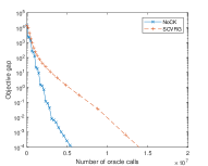
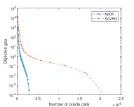
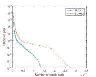
8 Conclusions

We have proposed an algorithm for solving the strongly convex case of the finite-sum compositional problem (1.1). To produce a stochastic $\varepsilon$-solution, the proposed algorithm generally needs $O\left((n_{1}+n_{2}+\kappa^{2.5})\log\frac{1}{\varepsilon}\right)$ evaluations of component function/gradient/Jacobian, where $\kappa$ denotes the condition number. For convex cases of (1.1), we proposed an algorithm that approximately solves a sequence of strongly convex perturbed problems. The complexity result is generally $O\left((n_{1}+n_{2})\log\frac{1}{\varepsilon}+\varepsilon^{-2.5}\right)$. Our complexity results are better than the existing best ones for general convex cases, and for strongly convex cases when $n_{1}+n_{2}>\kappa^{9/4}$ .

Appendix A Proof of Lemma 4.3

The following chain of inequalities holds:

$$\frac{(\tau_{1}+\tau_{2}-1+1/\theta-\overline{A}\tau_{1})\theta}{\tau_{2}+\overline{B}\tau_{1}}=\frac{(1+\frac{\tau_{2}}{\tau_{1}}-\overline{A})\tau_{1}\theta+1-\theta}{(\frac{\tau_{2}}{\tau_{1}}+\overline{B})\tau_{1}}\stackrel{{\scriptstyle\text{\char 172}}}{{=}}\frac{1+\frac{\tau_{2}}{\tau_{1}}-\overline{A}}{\frac{\tau_{2}}{\tau_{1}}+\overline{B}}\theta-\frac{1}{12m\tau_{1}(\frac{\tau_{2}}{\tau_{1}}+\overline{B})}$$

$$\stackrel{{\scriptstyle\text{\char 173}}}{{\geq}} 1+\frac{1-\overline{A}-\overline{B}}{\frac{\tau_{2}}{\tau_{1}}+\overline{B}}-\frac{1}{6(\frac{\tau_{2}}{\tau_{1}}+\overline{B})}=1+\frac{1-\overline{A}-\overline{B}-\frac{1}{6}}{\frac{\tau_{2}}{\tau_{1}}+\overline{B}}\stackrel{{\scriptstyle\text{\char 174}}}{{\geq}}1+\frac{1-\overline{A}-\overline{B}-\frac{1}{6}}{1+\overline{B}}\geq 1+\frac{1-\frac{1}{4}-\frac{1}{6}}{1+\frac{1}{8}}>\frac{13}{12}.$$

Here, ① holds because $\theta=1+\frac{1}{12m}$, ② follows from $\theta\geq 1$ and $2m\tau_{1}\geq 1$, and ③ uses $\frac{\tau_{2}}{\tau_{1}}\leq 1.$

Appendix B Results for multi-level finite-sum COP

In this section we extend SoCK and NoCK algorithms for a $p$-level finite-sum COP ($p\geq 2$) in the form of

$$\min_{x\in\mathbb{R}^{N_{1}}}H(x)\equiv\left(f_{p}\circ f_{p-1}\circ\cdots\circ f_{1}\right)(x)+h(x),$$ (B.1)

where $f_{i}=\frac{1}{n_{i}}\sum_{j=1}^{n_{i}}f_{i,j}$ is a finite-sum of $n_{i}$ differentiable maps $f_{i,j}\colon\mathbb{R}^{N_{i}}\rightarrow\mathbb{R}^{N_{i+1}}$ for all $i\in[p]$ and $j\in[n_{i}]$; and $h(x)$ is a convex regularizer that admits an easy proximal mapping. Clearly, only the last level $f_{p}$ must be a function with $N_{p+1}\equiv 1$. For consistency of notation, we write gradient information in terms of Jacobian matrices. As our results rely heavily on induction, we let $\phi^{\prime}$ denote the Jacobian matrix of map $\phi$, and define $\phi_{k}=f_{k}\circ f_{k-1}\circ\cdots\circ f_{1}$ for all $k\in[p]$. Then, by the chain rule,

$$\phi_{k}^{\prime}(x)=f_{k}^{\prime}(\phi_{k-1}(x))\cdot f_{k-1}^{\prime}(\phi_{k-2}(x))\cdots f_{1}^{\prime}(x)=f_{k}^{\prime}(\phi_{k-1}(x))\cdot\phi_{k-1}^{\prime}(x).$$ (B.2)

The critical component of the convergence of SoCK as well as the main difference it has from the convergence of Katyusha is the biased Jacobian estimation $\widetilde{\nabla}$ at a query point $x$ given a snapshot point $\widetilde{x}$, and how the bias ${\mathbb{E}}\|\widetilde{\nabla}-\phi_{p}^{\prime}(x)\|^{2}$ is bounded. Notice that the results in both Lemmas 4.1 and 5.1 are like

$${\mathbb{E}}\|\widetilde{\nabla}-\phi_{p}^{\prime}(x)\|^{2}=O\left(\|x-\widetilde{x}\|^{2}\cdot\sum\frac{1}{\text{mini-batch size}}\right),$$ (B.3)

and the success of SoCK is then from limiting this deviation from the Katyusha acceleration, so that all mini-batch sizes are set to $\Theta(\kappa^{2})$. For a $p$-level COP in (B.1), we can design a gradient estimator $\widetilde{\nabla}$ that achieves (B.3) and then implement it in SoCK. By this, everything else will follow exactly as those in Theorems 4.4 and 5.3.

Assumption B.1.

The function $\phi_{p}$ given in (B.1) is convex, and the function $h$ in (B.1) is $\mu$-strongly convex with $\mu>0$.

Assumption B.2.

For every $i\in[p]$ $j\in[n_{i}]$, $f_{i,j}\colon\mathbb{R}^{N_{i}}\rightarrow\mathbb{R}^{N_{i+1}}$ is $L_{i}$-smooth and has a $B_{i}$-bounded Jacobian matrix. Also, $\phi_{p}$ is $L$-smooth.

With Assumption B.2, it is known that $\phi_{k}$ is $\ell_{k}$-smooth and has a $\gamma_{k}$-bounded Jacobian matrix, where $\gamma_{k}=\prod_{i=1}^{k}B_{i}$ and $\ell_{k}=\sum_{i=1}^{k}L_{i}(\prod_{j=1}^{i-1}B_{j}^{2})(\prod_{j=i+1}^{k}B_{j})$; cf. zhang2019multi . To be consistent with the notation of SoCK, we still use $L$ as the smoothness parameter of $\phi_{p}$, and hence $L\leq\ell_{p}$. In practice $\ell_{p}$ may not be well-defined, or may dominate a good estimate of $L$. In this section we will utilize the fact that $f_{k,j}\circ\phi_{k-1}$ is also $\ell_{k}$-smooth.

For a $p$-level composition, we replace the snapshot computation and gradient estimation of SoCK as follows and obtain Algorithm 3. At a snapshot point $\widetilde{x}$, we compute

$$\phi_{1}(\widetilde{x}),\ldots,\,\phi_{k}(\widetilde{x}),\ldots,\,\phi_{p-1}(\widetilde{x})$$ (B.4)

and

$$f_{1}^{\prime}(\widetilde{x}),\,f_{2}^{\prime}(\phi_{1}(\widetilde{x})),\ldots,\,f_{k+1}^{\prime}(\phi_{k}(\widetilde{x})),\ldots,\,f_{p}^{\prime}(\phi_{p-1}(\widetilde{x})).$$ (B.5)

Hence, by (B.2), we can also compute

$$\phi_{1}^{\prime}(\widetilde{x}),\ldots,\,\phi_{k}^{\prime}(\widetilde{x}),\ldots,\,\phi_{p}^{\prime}(\widetilde{x}).$$ (B.6)

For any query-snapshot pair $(x,\widetilde{x})$, compute the inner map and Jacobian estimations inductively

$$u_{1}=\frac{1}{a_{1}}\sum_{j\in\hbox{$\mathcal{A}$}_{1}}\left(f_{1,j}(x)-f_{1,j}(\widetilde{x})\right)+\phi_{1}(\widetilde{x})\text{ and }v_{1}=\frac{1}{b_{1}}\sum_{j\in\hbox{$\mathcal{B}$}_{1}}\left(f_{1,j}^{\prime}(x)-f_{1,j}^{\prime}(\widetilde{x})\right)+\phi_{1}^{\prime}(\widetilde{x}),$$ (B.7)

where $\hbox{$\mathcal{A}$}_{1}$ and $\hbox{$\mathcal{B}$}_{1}$ are sampled uniformly at random from $[n_{1}]$ with replacement such that $|\hbox{$\mathcal{A}$}_{1}|=a_{1}$ and $|\hbox{$\mathcal{B}$}_{1}|=b_{1}$. For $k=2,\ldots,p$, we compute the inner map estimation

$$u_{k}=\frac{1}{a_{k}}\sum_{j\in\hbox{$\mathcal{A}$}_{k}}\left(f_{k,j}(u_{k-1})-f_{k,j}(\phi_{k-1}(\widetilde{x}))\right)+\phi_{k}(\widetilde{x})$$ (B.8)

and the Jacobian estimation

$$v_{k}=\frac{1}{b_{k}}\sum_{j\in\hbox{$\mathcal{B}$}_{k}}\left(f_{k,j}^{\prime}(u_{k-1})v_{k-1}-f_{k,j}^{\prime}(\phi_{k-1}(\widetilde{x}))\phi_{k-1}^{\prime}(\widetilde{x})\right)+\phi_{k}^{\prime}(\widetilde{x}),$$ (B.9)

where $\hbox{$\mathcal{A}$}_{k}$ and $\hbox{$\mathcal{B}$}_{k}$ are sampled uniformly at random from $[n_{k}]$ with replacement such that $|\hbox{$\mathcal{A}$}_{k}|=a_{k}$ and $|\hbox{$\mathcal{B}$}_{k}|=b_{k}$. We return $\widetilde{\nabla}=v_{p}^{\top}$ as the gradient estimation.

Algorithm 3 Multi-level SoCK

Input: $x_{0}\in\mathbb{R}^{N_{1}},$ $S,$ $m\leq\frac{L}{2\mu},$ $\theta>1$, mini-batch sizes $\{a_{i}\}_{i=1}^{p-1}$ and $\{b_{i}\}_{i=1}^{p}$;

Let $y_{0}=z_{0}=\widetilde{x}^{0}\leftarrow x_{0};$

for $s=0$ to $S-1$ do

    Compute (B.4), (B.5), and (B.6); $\triangleright$ take a snapshot

    for $j=0$ to $m-1$ do

         $k\leftarrow sm+j;$

         $x_{k+1}\leftarrow\tau_{1}z_{k}+\tau_{2}\widetilde{x}^{s}+(1-\tau_{1}-\tau_{2})y_{k};$ $\triangleright$ linear coupling step

         Compute $v_{p}(x_{k+1},\widetilde{x}^{s})$ by (B.7), (B.8), and (B.9);

         Update $\textstyle\widetilde{\nabla}_{k+1}\leftarrow[v_{p}(x_{k+1},\widetilde{x}^{s})]^{\top}$; $\triangleright$ biased gradient estimator

         Let $z_{k+1}\leftarrow\operatorname*{arg\,min}_{z}\,\langle\widetilde{\nabla}_{k+1},z\rangle+\frac{1}{2\alpha}\|z-z_{k}\|^{2}+h(z);$ $\triangleright$ mirror descent step

         Let $y_{k+1}\leftarrow\operatorname*{arg\,min}_{y}\,\langle\widetilde{\nabla}_{k+1},y\rangle+\frac{3L}{2}\|y-x_{k+1}\|^{2}+h(y);$ $\triangleright$ gradient descent step

    end for

    $\widetilde{x}^{s+1}\leftarrow(\sum_{j=0}^{m-1}\theta^{j})^{-1}\cdot\sum_{j=0}^{m-1}\theta^{j}y_{sm+j+1};$ $\triangleright$ update to the snapshot point

end for

return $\widetilde{x}^{S}$.

Below, we establish (B.3). In order to do this, we bound ${\mathbb{E}}\|\widetilde{\nabla}-\phi_{p}^{\prime}(x)\|^{2}={\mathbb{E}}\|v_{p}-\phi_{p}^{\prime}(x)\|^{2}$ by forming recurrence relations.

Lemma B.1.

Let the query point $x$ and the snapshot point $\widetilde{x}$ be given, and $\widetilde{\nabla}=v_{p}$ be computed by (B.7), (B.8), and (B.9). Then under Assumption B.2,

$${\mathbb{E}}[\|\widetilde{\nabla}-\phi_{p}^{\prime}(x)\|^{2}|x,\widetilde{x}]\leq\left(\sum_{j=1}^{p}\frac{2}{b_{j}}\frac{4^{p-j}\ell_{j}^{2}\gamma_{p}^{2}}{\gamma_{j}^{2}}+\sum_{i=1}^{p-1}\frac{1}{a_{i}}\sum_{j=i+1}^{p}\frac{4^{p-j+1}\gamma_{p}^{2}\gamma_{j-1}^{4}L_{j}^{2}}{\gamma_{j}^{2}}\right)\|x-\widetilde{x}\|^{2}.$$ (B.10)

Proof.

The first recurrence on ${\mathbb{E}}\|v_{k}-\phi_{k}^{\prime}(x)\|^{2}$ is follows the proof of Lemma 5.1.

$$\|v_{k}-\phi_{k}^{\prime}(x)\|^{2}\leq 2\left\|v_{k}-\frac{1}{b_{k}}\sum_{j\in\hbox{$\mathcal{B}$}_{k}}\left(f_{k,j}^{\prime}(\phi_{k-1}(x))\phi_{k-1}^{\prime}(x)-f_{k,j}^{\prime}(\phi_{k-1}(\widetilde{x}))\phi_{k-1}^{\prime}(\widetilde{x})\right)-\phi_{k}^{\prime}(\widetilde{x})\right\|^{2}$$

$$+2\left\|\frac{1}{b_{k}}\sum_{j\in\hbox{$\mathcal{B}$}_{k}}\left(f_{k,j}^{\prime}(\phi_{k-1}(x))\phi_{k-1}^{\prime}(x)-f_{k,j}^{\prime}(\phi_{k-1}(\widetilde{x}))\phi_{k-1}^{\prime}(\widetilde{x})\right)+\phi_{k}^{\prime}(\widetilde{x})-\phi_{k}^{\prime}(x)\right\|^{2}.$$ (B.11)

The first term of the r.h.s. of (B.11) can be simplified and bounded as follows,

$$\left\|v_{k}-\frac{1}{b_{k}}\sum_{j\in\hbox{$\mathcal{B}$}_{k}}\left(f_{k,j}^{\prime}(\phi_{k-1}(x))\phi_{k-1}^{\prime}(x)-f_{k,j}^{\prime}(\phi_{k-1}(\widetilde{x}))\phi_{k-1}^{\prime}(\widetilde{x})\right)-\phi_{k}^{\prime}(\widetilde{x})\right\|^{2}$$

$$= \frac{1}{b_{k}^{2}}\left\|\sum_{j\in\hbox{$\mathcal{B}$}_{k}}\left(f_{k,j}^{\prime}(u_{k-1})v_{k-1}-f_{k,j}^{\prime}(\phi_{k-1}(x))\phi_{k-1}^{\prime}(x)\right)\right\|^{2}$$

$$\leq \frac{1}{b_{k}}\sum_{j\in\hbox{$\mathcal{B}$}_{k}}\left\|f_{k,j}^{\prime}(u_{k-1})v_{k-1}-f_{k,j}^{\prime}(\phi_{k-1}(x))\phi_{k-1}^{\prime}(x)\right\|^{2}$$

$$\leq \frac{1}{b_{k}}\sum_{j\in\hbox{$\mathcal{B}$}_{k}}2\left\|f_{k,j}^{\prime}(u_{k-1})v_{k-1}-f_{k,j}^{\prime}(u_{k-1})\phi_{k-1}^{\prime}(x)\right\|^{2}+2\left\|f_{k,j}^{\prime}(u_{k-1})\phi_{k-1}^{\prime}(x)-f_{k,j}^{\prime}(\phi_{k-1}(x))\phi_{k-1}^{\prime}(x)\right\|^{2}$$

$$\leq 2B_{k}^{2}\left\|v_{k-1}-\phi_{k-1}^{\prime}(x)\right\|^{2}+2\gamma_{k-1}^{2}L_{k}^{2}\left\|u_{k-1}-\phi_{k-1}(x)\right\|^{2},$$

where the equality follows from (B.9), the first and second inequalities use Cauchy-Schwarz inequaity, and the last inequality follows from the boundedness of $f_{k,j}^{\prime}$ and $\phi_{k-1}^{\prime}$, and the $L_{k}$-smoothness of $f_{k,j}^{\prime}$. The second term of the r.h.s. of (B.11) can be bounded by the same process for the second term of the r.h.s. of (5.3), by using the $\ell_{k}$-smoothness of each $f_{k,j}\circ\phi_{k-1}$, and it results in

$${\mathbb{E}}\left[\left\|\frac{1}{b_{k}}\sum_{j\in\hbox{$\mathcal{B}$}_{k}}\left(f_{k,j}^{\prime}(\phi_{k-1}(x))\phi_{k-1}^{\prime}(x)-f_{k,j}^{\prime}(\phi_{k-1}(\widetilde{x}))\phi_{k-1}^{\prime}(\widetilde{x})\right)+\phi_{k}^{\prime}(\widetilde{x})-\phi_{k}^{\prime}(x)\right\|^{2}\nonscript\;\middle|\nonscript\;x,\widetilde{x}\right]\leq\frac{\ell_{k}^{2}}{b_{k}}\|x-\widetilde{x}\|^{2}.$$

Utilizing the above two bounds for (B.11), we have the first recurrence relation

$${\mathbb{E}}[\|v_{k}-\phi_{k}^{\prime}(x)\|^{2}|x,\widetilde{x}]\leq 4B_{k}^{2}{\mathbb{E}}[\|v_{k-1}-\phi_{k-1}^{\prime}(x)\|^{2}|x,\widetilde{x}]+4\gamma_{k-1}^{2}L_{k}^{2}{\mathbb{E}}[\|u_{k-1}-\phi_{k-1}(x)\|^{2}|x,\widetilde{x}]+\frac{2\ell_{k}^{2}}{b_{k}}\|x-\widetilde{x}\|^{2}.$$ (B.12)

We establish the recurrence for $\|u_{k}-\phi_{k}(x)\|^{2}$ as follows,

$${\mathbb{E}}[\|u_{k}-\phi_{k}(x)\|^{2}|x,\widetilde{x},u_{k-1}]$$ (B.13)

$$= {\frac{1}{a_{k}^{2}}{\mathbb{E}}\left[\left\|\sum_{j\in\hbox{$\mathcal{A}$}_{k}}\left(f_{k,j}(u_{k-1})-f_{k,j}(\phi_{k-1}(\widetilde{x}))+\phi_{k}(\widetilde{x})-\phi_{k}(x)\right)\right\|^{2}\nonscript\;\middle|\nonscript\;x,\widetilde{x},u_{k-1}\right]}$$ (B.14)

$$= {\frac{1}{a_{k}^{2}}{\mathbb{E}}\left[\left\|\sum_{j\in\hbox{$\mathcal{A}$}_{k}}\left(f_{k,j}(u_{k-1})-f_{k,j}(\phi_{k-1}(\widetilde{x}))-f_{k}(u_{k-1})+\phi_{k}(\widetilde{x})+f_{k}(u_{k-1})-\phi_{k}(x)\right)\right\|^{2}\nonscript\;\middle|\nonscript\;x,\widetilde{x},u_{k-1}\right]}$$ (B.15)

$$= \frac{1}{a_{k}^{2}}\sum_{j\in\hbox{$\mathcal{A}$}_{k}}{\mathbb{E}}[\|f_{k,j}(u_{k-1})-f_{k,j}(\phi_{k-1}(\widetilde{x}))-f_{k}(u_{k-1})+\phi_{k}(\widetilde{x})\|^{2}|x,\widetilde{x},u_{k-1}]+\|f_{k}(u_{k-1})-\phi_{k}(x)\|^{2}$$ (B.16)

$$\leq \frac{1}{a_{k}^{2}}\sum_{j\in\hbox{$\mathcal{A}$}_{k}}{\mathbb{E}}[\|f_{k,j}(u_{k-1})-f_{k,j}(\phi_{k-1}(\widetilde{x}))\|^{2}|x,\widetilde{x},u_{k-1}]+\|f_{k}(u_{k-1})-\phi_{k}(x)\|^{2}$$ (B.17)

$$\leq \frac{B_{k}^{2}}{a_{k}}\left\|u_{k-1}-\phi_{k-1}(\widetilde{x})\right\|^{2}+B_{k}^{2}\left\|u_{k-1}-\phi_{k-1}(x)\right\|^{2},$$ (B.18)

where the first equality follows from (B.8), the third equality comes from the fact that $\big{\{}f_{k,j}(u_{k-1})-f_{k,j}(\phi_{k-1}(\widetilde{x}))-f_{k}(u_{k-1})+\phi_{k}(\widetilde{x})\big{\}}$ are conditionally independent with each other, and their expectations all equal 0, the first inequality holds because the variance is bounded by the second moment, and the second inequality follows from the intermediate value theorem and the boundedness of the Jacobian of each $f_{k,j}$ and $f_{k}$. A similar argument gives us the following recurrence for $\|u_{k}-\phi_{k}(\widetilde{x})\|^{2}$:

$$\|u_{k}-\phi_{k}(\widetilde{x})\|^{2}= \frac{1}{a_{k}^{2}}\left\|\sum_{j\in\hbox{$\mathcal{A}$}_{k}}\left(f_{k,j}(u_{k-1})-f_{k,j}(\phi_{k-1}(\widetilde{x}))\right)\right\|^{2}$$ (B.19)

$$\leq \frac{1}{a_{k}}\sum_{j\in\hbox{$\mathcal{A}$}_{k}}\|f_{k,j}(u_{k-1})-f_{k,j}(\phi_{k-1}(\widetilde{x}))\|^{2}\leq B_{k}^{2}\left\|u_{k-1}-\phi_{k-1}(x)\right\|^{2},$$ (B.20)

where the first inequality uses Cauchy-Schwarz inequaity, and the second inequality follows from the intermediate value theorem and the $B_{k}$-boundedness of the Jacobian of each $f_{k,j}$. Also note that by the same argument as that of (B.20), we have $\|u_{1}-\phi_{1}(\widetilde{x})\|^{2}\leq B_{1}^{2}\|x-\widetilde{x}\|^{2}$, which together with (B.20) implies that for all $k\in[p]$,

$$\|u_{k}-\phi_{k}(\widetilde{x})\|^{2}\leq\gamma_{k}^{2}\|x-\widetilde{x}\|^{2}.$$ (B.21)

Plugging (B.21) into (B.18), we obtain the recurrence

$${\mathbb{E}}[\|u_{k}-\phi_{k}(x)\|^{2}|x,\widetilde{x}]\leq B_{k}^{2}{\mathbb{E}}[\|u_{k-1}-\phi_{k-1}(x)\|^{2}|x,\widetilde{x}]+\frac{\gamma_{k}^{2}}{a_{k}}\|x-\widetilde{x}\|^{2};$$

together with the fact that ${\mathbb{E}}[\|u_{1}-\phi_{1}(x)\|^{2}|x,\widetilde{x}]\leq\frac{B_{1}^{2}}{a_{1}}\|x-\widetilde{x}\|^{2}$, which is similar to (3.5), we have

$${\mathbb{E}}[\|u_{k}-\phi_{k}(x)\|^{2}|x,\widetilde{x}]\leq\gamma_{k}^{2}\left(\sum_{i=1}^{k}\frac{1}{a_{i}}\right)\|x-\widetilde{x}\|^{2}.$$ (B.22)

Plug (B.22) into (B.12) to obtain the recurrence

$${\mathbb{E}}[\|v_{k}-\phi_{k}^{\prime}(x)\|^{2}|x,\widetilde{x}]\leq 4B_{k}^{2}{\mathbb{E}}[\|v_{k-1}-\phi_{k-1}^{\prime}(x)\|^{2}|x,\widetilde{x}]+\left(4\gamma_{k-1}^{4}L_{k}^{2}\sum_{i=1}^{k-1}\frac{1}{a_{i}}+\frac{2\ell_{k}^{2}}{b_{k}}\right)\|x-\widetilde{x}\|^{2};$$

together with the fact that ${\mathbb{E}}[\|v_{1}-\phi_{1}^{\prime}(x)\|^{2}|x,\widetilde{x}]\leq\frac{L_{1}^{2}}{b_{1}}\|x-\widetilde{x}\|^{2}$, which appeared right after (3.5) , we have

$${\mathbb{E}}[\|v_{k}-\phi_{k}^{\prime}(x)\|^{2}|x,\widetilde{x}]\leq \|x-\widetilde{x}\|^{2}4^{k}\gamma_{k}^{2}\sum_{j=1}^{k}\frac{1}{4^{j}\gamma_{j}^{2}}\left(\frac{2\ell_{j}^{2}}{b_{j}}+4\gamma_{j-1}^{4}L_{j}^{2}\sum_{i=1}^{j-1}\frac{1}{a_{i}}\right)$$

$$= \left(\sum_{j=1}^{k}\frac{2}{b_{j}}\frac{4^{k-j}\ell_{j}^{2}\gamma_{k}^{2}}{\gamma_{j}^{2}}+\sum_{i=1}^{k-1}\frac{1}{a_{i}}\sum_{j=i+1}^{k}\frac{4^{k-j+1}\gamma_{k}^{2}\gamma_{j-1}^{4}L_{j}^{2}}{\gamma_{j}^{2}}\right)\|x-\widetilde{x}\|^{2}.$$

Let $k=p$ in the above completes the proof. ∎

Plugging (B.10) into (3.15), we are able to show (3.18) and thus (3.19) with an appropriate $M$.

Lemma B.2.

Suppose $\tau_{1}\in(0,\frac{1}{3\alpha L}]$ and $\tau_{2}\in[0,1-\tau_{1}]$ in the linear coupling step of Algorithm 3. Let $x^{*}$ be the solution of (B.1). If $\widetilde{\nabla}_{k+1}$ is computed by (B.7), (B.8), and (B.9), then (3.18) holds with

$$M=3\Big{(}\frac{1}{4\tau_{1}L}+\frac{3}{\mu}\Big{)}\left(\sum_{j=1}^{p}\frac{2}{b_{j}}\frac{4^{p-j}\ell_{j}^{2}\gamma_{p}^{2}}{\gamma_{j}^{2}}+\sum_{i=1}^{p-1}\frac{1}{a_{i}}\sum_{j=i+1}^{p}\frac{4^{p-j+1}\gamma_{p}^{2}\gamma_{j-1}^{4}L_{j}^{2}}{\gamma_{j}^{2}}\right).$$ (B.23)

Proof.

Taking conditional expectation ${\mathbb{E}}_{k-1}$ on both sides of (3.15) with $\beta=\frac{6}{\mu}$ and plugging (B.10), we immediately have (3.18) by using the choice of $M$ in (B.23). ∎

The convergence of Algorithm 3 follows that of Algorithm 1, based on Lemma B.2 and a similar parameter choice.

Theorem B.3 (convergence result for multi-level SoCK).

Under Assumptions B.1 and B.2, let $\{\widetilde{x}^{s}\}$ be generated from Algorithm 3 with $\widetilde{\nabla}_{k+1}$ computed by (B.7), (B.8), (B.9) and with parameters set as follows:

$$m\leftarrow\left\lceil\frac{1}{2}\sqrt{\frac{L}{\mu}}\right\rceil,\,\tau_{1}\leftarrow\frac{1}{2m},\,\tau_{2}\leftarrow\frac{1}{2m},\,\theta\leftarrow 1+\frac{1}{12m},\,\alpha\leftarrow\frac{1}{3\tau_{1}L},$$ (B.24a)

$$a_{i}\leftarrow\frac{180(2p-1)}{\mu^{2}}\sum_{j=i+1}^{p}\frac{4^{p-j+1}\gamma_{p}^{2}\gamma_{j-1}^{4}L_{j}^{2}}{\gamma_{j}^{2}}\quad\text{ for }i=1,\ldots,p-1,$$ (B.24b)

$$b_{i}\leftarrow\frac{360(2p-1)}{\mu^{2}}\frac{4^{p-i}\ell_{i}^{2}\gamma_{p}^{2}}{\gamma_{i}^{2}}\quad\text{ for }i=1,\ldots,p.$$ (B.24c)

Then

$$\operatorname{\mathbb{E}}\big{[}H(\widetilde{x}^{S})-H(x^{\ast})\big{]}\leq 11\cdot\left(\frac{12}{13}\right)^{S}\big{(}H(x_{0})-H(x^{\ast})\big{)}.$$

Proof.

Notice that the parameters given in (B.24) are the same as those in (4.3) except for $\{a_{i}\}_{i=1}^{p-1}$ and $\{b_{i}\}_{i=1}^{p}$, and also notice that the choices of $\{a_{i}\}_{i=1}^{p-1}$ and $\{b_{i}\}_{i=1}^{p}$ only affect the value of $M$. Plugging into (B.23) the values of $\{a_{i}\}_{i=1}^{p-1}$ and $\{b_{i}\}_{i=1}^{p}$ given in (B.24b) and (B.24c), we can easily verify that $M\leq\frac{\mu}{16}$. Now following the same arguments in the proof of Theorem 4.4, we obtain the desired result. ∎

By Theorem B.3, we can estimate the complexity of Algorithm 3 in terms of the number of evaluations on $f_{i,j}$, $f_{i,j}^{\prime}$, and the proximal mapping of $h$. Its proof follows that of Corollary 4.5, and we omit it.

Corollary B.4.

Given $\varepsilon>0$, under the same assumptions as those in Theorem B.3, the number of component map/Jacobian evaluations of Algorithm 3 to produce a stochastic $\varepsilon$-solution is

$$O\left(\Big{(}\sum_{i=1}^{p}n_{i}+\sqrt{\frac{L}{\mu}}\frac{\ell_{p}^{2}}{\mu^{2}}\Big{)}\log\frac{H(x_{0})-H(x^{\ast})}{\varepsilon}\right).$$

The extension to a $p$-level finite-sum COP (B.1) that is non-strongly convex can be done easily, following the argument in Section 6, hence we omit the details.

Appendix C More numerical tests

In this section, we provide more numerical results, which can show the stable performance of the proposed methods. In Figures 3 and 4, we compare Algorithm 1 with both options to VRSC-PG in huo2018accelerated , C-SAGA and GC-SAGA in zhang2019composite on four independent trials with different $n$ and $\kappa$. In Figures 5, 6, 7 and 8, we compare Algorithm 2 to SCVRG in lin2018improved on four independent trials with different $n$ but similar smoothness constant $L$.

Figure 3: Comparison of the proposed SOCK (i.e., Algorithm 1 with Option I) and GOCK (i.e., Algorithm 1 with Option II) to VRSC-PG in huo2018accelerated , C-SAGA and GC-SAGA in zhang2019composite on solving instances of (7.1) having $\kappa>(2n)^{9/4}$, with the parameter tuple $(n,\kappa,v)=(5e3,96,30)$ in the top row and $(n,\kappa,v)=(5e4,211,10)$ in the bottom row. All methods take the explicitly-computed strong convexity constant $\mu$. The value of $v$ is varied to change the condition number $\kappa$.

trial $1$	trial $2$	trial $3$	trial $4$

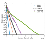
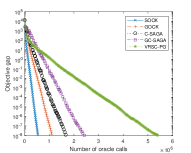
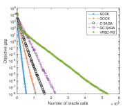
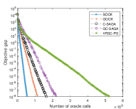
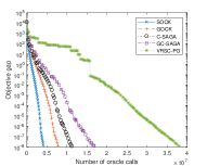
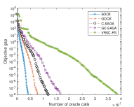
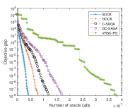
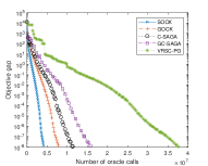
Figure 4: Comparison of the proposed SOCK (i.e., Algorithm 1 with Option I) and GOCK (i.e., Algorithm 1 with Option II) to VRSC-PG in huo2018accelerated , C-SAGA and GC-SAGA in zhang2019composite on solving instances of (7.1) having $(2n)^{1/3}<\kappa<(2n)^{4/9}$, with the parameter tuple $(n,\kappa,v)=(5e3,52,60)$ in the top row and $(n,\kappa,v)=(5e4,93,30)$ in the bottom row. All methods take the explicitly-computed strong convexity constant $\mu$. The value of $v$ is varied to change the condition number $\kappa$.

trial $1$	trial $2$	trial $3$	trial $4$

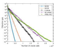
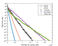
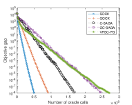
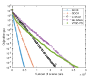
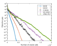
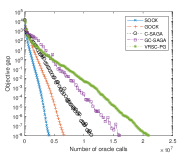
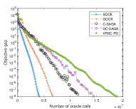
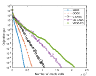
Figure 5: Comparison of the proposed NoCK method (i.e., Algorithm 2) to SCVRG in lin2018improved on solving instances of (7.1) with the parameter tuple $(n,L,v)=(5e4,791,0)$. The instances are treated as convex, even though they can be strongly convex. Parameters of the algorithms are set by the theoretical parameter choice in the top row and the heuristic choice in the bottom row.

trial $1$	trial $2$	trial $3$	trial $4$

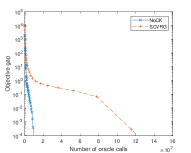
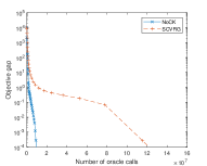
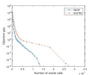
Figure 6: Comparison of the proposed NoCK method (i.e., Algorithm 2) to SCVRG in lin2018improved on solving instances of (7.1) with the parameter tuple $(n,L,v)=(2.5e5,806,0)$. The instances are treated as convex, even though they can be strongly convex. Parameters of the algorithms are set by the theoretical parameter choice in the top row and the heuristic choice in the bottom row.

trial $1$	trial $2$	trial $3$	trial $4$

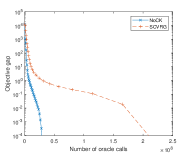
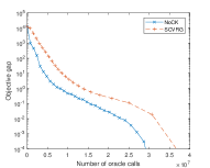
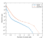
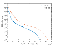
Figure 7: Comparison of the proposed NoCK method (i.e., Algorithm 2) to SCVRG in lin2018improved on solving instances of (7.1) with the parameter tuple $(n,L,v)=(5e4,798,10)$. The instances are treated as convex, even though they can be strongly convex. Parameters of the algorithms are set by the theoretical parameter choice in the top row and the heuristic choice in the bottom row.

trial $1$	trial $2$	trial $3$	trial $4$

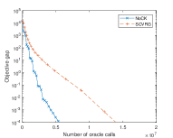
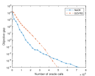
Figure 8: Comparison of the proposed NoCK method (i.e., Algorithm 2) to SCVRG in lin2018improved on solving instances of (7.1) with the parameter tuple $(n,L,v)=(2.5e5,799,10)$. The instances are treated as convex, even though they can be strongly convex. Parameters of the algorithms are set by the theoretical parameter choice in the top row and the heuristic choice in the bottom row.

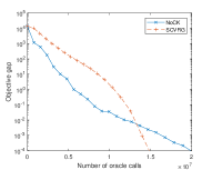
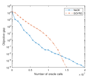
trial $1$	trial $2$	trial $3$	trial $4$

References

• [1] Z. Allen-Zhu. Katyusha: The first direct acceleration of stochastic gradient methods. The Journal of Machine Learning Research, 18(1):8194–8244, 2017.
• [2] Z. Allen-Zhu and E. Hazan. Optimal black-box reductions between optimization objectives. In D. D. Lee, M. Sugiyama, U. V. Luxburg, I. Guyon, and R. Garnett, editors, Advances in Neural Information Processing Systems 29, pages 1614–1622. Curran Associates, Inc., 2016.
• [3] Z. Allen-Zhu and L. Orecchia. Linear coupling: An ultimate unification of gradient and mirror descent. arXiv preprint arXiv:1407.1537, 2014.
• [4] Z. Chen and Y. Zhou. Momentum with variance reduction for nonconvex composition optimization. arXiv preprint arXiv:2005.07755, 2020.
• [5] A. Defazio. A simple practical accelerated method for finite sums. In D. D. Lee, M. Sugiyama, U. V. Luxburg, I. Guyon, and R. Garnett, editors, Advances in Neural Information Processing Systems 29, pages 676–684. Curran Associates, Inc., 2016.
• [6] A. Defazio, F. Bach, and S. Lacoste-Julien. Saga: A fast incremental gradient method with support for non-strongly convex composite objectives. In Z. Ghahramani, M. Welling, C. Cortes, N. D. Lawrence, and K. Q. Weinberger, editors, Advances in Neural Information Processing Systems 27, pages 1646–1654. Curran Associates, Inc., 2014.
• [7] S. Ghadimi, A. Ruszczynski, and M. Wang. A single timescale stochastic approximation method for nested stochastic optimization. SIAM Journal on Optimization, 30(1):960–979, 2020.
• [8] Z. Huo, B. Gu, J. Liu, and H. Huang. Accelerated Method for Stochastic Composition Optimization With Nonsmooth Regularization. In Thirty-Second AAAI Conference on Artificial Intelligence, New Orleans, LA, USA, 2–7 Feburary 2018.
• [9] R. Johnson and T. Zhang. Accelerating stochastic gradient descent using predictive variance reduction. In C. J. C. Burges, L. Bottou, M. Welling, Z. Ghahramani, and K. Q. Weinberger, editors, Advances in Neural Information Processing Systems 26, pages 315–323. Curran Associates, Inc., 2013.
• [10] G. Lan. First-order and Stochastic Optimization Methods for Machine Learning. Springer, 2020.
• [11] X. Lian, M. Wang, and J. Liu. Finite-sum Composition Optimization via Variance Reduced Gradient Descent. volume 54 of Proceedings of Machine Learning Research, pages 1159–1167, Fort Lauderdale, FL, USA, 20–22 Apr 2017. PMLR.
• [12] H. Lin, J. Mairal, and Z. Harchaoui. A universal catalyst for first-order optimization. In C. Cortes, N. D. Lawrence, D. D. Lee, M. Sugiyama, and R. Garnett, editors, Advances in Neural Information Processing Systems 28, pages 3384–3392. Curran Associates, Inc., 2015.
• [13] T. Lin, C. Fan, M. Wang, and M. I. Jordan. Improved sample complexity for stochastic compositional variance reduced gradient. In 2020 American Control Conference (ACC), pages 126–131, 2020.
• [14] L. Liu, J. Liu, and D. Tao. Variance reduced methods for non-convex composition optimization. arXiv preprint arXiv:1711.04416, 2017.
• [15] H. Markowitz. Portfolio selection [reprint of J. Finance 7 (1952), no. 1, 77–91]. In Financial risk measurement and management, volume 267 of Internat. Lib. Crit. Writ. Econ., pages 197–211. Edward Elgar, Cheltenham, 2012.
• [16] H. M. Markowitz. Mean-variance analysis in portfolio choice and capital markets. Basil Blackwell, Oxford, 1987.
• [17] Y. Nesterov. Gradient methods for minimizing composite functions. Mathematical Programming, 140(1):125–161, 2013.
• [18] Y. Nesterov. Introductory lectures on convex optimization: A basic course, volume 87. Springer Science & Business Media, 2013.
• [19] Y. E. Nesterov. A method for solving the convex programming problem with convergence rate o (1/k^ 2). In Dokl. akad. nauk Sssr, volume 269, pages 543–547, 1983.
• [20] P. Rigollet and X. Tong. Neyman-pearson classification, convexity and stochastic constraints. Journal of Machine Learning Research, 12(Oct):2831–2855, 2011.
• [21] M. Schmidt, N. Le Roux, and F. Bach. Minimizing finite sums with the stochastic average gradient. Mathematical Programming, 162(1-2):83–112, 2017.
• [22] F. Shang, L. Jiao, K. Zhou, J. Cheng, Y. Ren, and Y. Jin. Asvrg: Accelerated proximal svrg. volume 95 of Proceedings of Machine Learning Research, pages 815–830. PMLR, 14–16 Nov 2018.
• [23] Q. Tran-Dinh, N. Pham, and L. Nguyen. Stochastic Gauss-Newton algorithms for nonconvex compositional optimization. In H. D. III and A. Singh, editors, Proceedings of the 37th International Conference on Machine Learning, volume 119 of Proceedings of Machine Learning Research, pages 9572–9582, Virtual, 13–18 Jul 2020. PMLR.
• [24] M. Wang, E. X. Fang, and H. Liu. Stochastic compositional gradient descent: algorithms for minimizing compositions of expected-value functions. Mathematical Programming, 161(1-2):419–449, 2017.
• [25] M. Wang, J. Liu, and E. X. Fang. Accelerating stochastic composition optimization. Journal of Machine Learning Research, 18(105):1–23, 2017.
• [26] B. E. Woodworth and N. Srebro. Tight complexity bounds for optimizing composite objectives. In D. D. Lee, M. Sugiyama, U. V. Luxburg, I. Guyon, and R. Garnett, editors, Advances in Neural Information Processing Systems 29, pages 3639–3647. Curran Associates, Inc., 2016.
• [27] L. Xiao and T. Zhang. A proximal stochastic gradient method with progressive variance reduction. SIAM Journal on Optimization, 24(4):2057–2075, 2014.
• [28] Y. Xu. Iteration complexity of inexact augmented lagrangian methods for constrained convex programming. Mathematical Programming, Series A, 185:199–244, 2021.
• [29] S. Yang, M. Wang, and E. X. Fang. Multilevel stochastic gradient methods for nested composition optimization. SIAM Journal on Optimization, 29(1):616–659, 2019.
• [30] Y. Yu and L. Huang. Fast stochastic variance reduced admm for stochastic composition optimization. In Proceedings of the Twenty-Sixth International Joint Conference on Artificial Intelligence, IJCAI-17, pages 3364–3370, 2017.
• [31] M. B. Zafar, I. Valera, M. G. Rogriguez, and K. P. Gummadi. Fairness Constraints: Mechanisms for Fair Classification. volume 54 of Proceedings of Machine Learning Research, pages 962–970, Fort Lauderdale, FL, USA, 20–22 Apr 2017. PMLR.
• [32] J. Zhang and L. Xiao. A composite randomized incremental gradient method. volume 97 of Proceedings of Machine Learning Research, pages 7454–7462, Long Beach, California, USA, 09–15 Jun 2019. PMLR.
• [33] J. Zhang and L. Xiao. Multi-level composite stochastic optimization via nested variance reduction. arXiv preprint arXiv:1908.11468, 2019.
• [34] J. Zhang and L. Xiao. Stochastic variance-reduced prox-linear algorithms for nonconvex composite optimization. arXiv preprint arXiv:2004.04357, 2020.