High dimensional regression for regenerative time-series: an application to road traffic modeling

Mohammed Bouchouia and François Portier

Télécom Paris, Institut Polytechnique de Paris
Abstract

A statistical predictive model in which a high-dimensional time-series regenerates at the end of each day is used to model road traffic. Due to the regeneration, prediction is based on a daily modeling using a vector autoregressive model that combines linearly the past observations of the day. Due to the high-dimension, the learning algorithm follows from an 1subscript1\ell_{1}-penalization of the regression coefficients. Excess risk bounds are established under the high-dimensional framework in which the number of road sections goes to infinity with the number of observed days. Considering floating car data observed in an urban area, the approach is compared to state-of-the-art methods including neural networks. In addition of being highly competitive in terms of prediction, it enables the identification of the most determinant sections of the road network.

Keywords— MSC 2010 subject classifications: Primary 62J05, 62J07, ; secondary 62P30.

vector autoregressive model, Lasso, regenerative process, road traffic prediction

1 Introduction

As the world witnesses the negative effects of traffic congestion, including pollution and economically ineffective transportation (Bull, , 2003; Pellicer et al., , 2013; Harrison and Donnelly, , 2011), achieving smart mobility has become one of the leading challenges of emerging cities (Washburn et al., , 2009). In order to set up effective solutions, such as developing intelligent transportation management systems for urban planners, or extending the road network efficiently, smart cities first need to accurately understand road traffic. This paper investigates interpretable predictive models estimated from floating car data, allowing for the identification of road traffic determinants.

The proposed methodology addresses two important issues regarding floating car data. First, in contrast with a traditional time series analysis (Brockwell et al., , 1991), the number of vehicles using the network almost vanishes during the night. Hence, in terms of probabilistic dependency, the road traffic between the different days is assumed independent. Such a phenomenon is referred to as “regeneration” in the Markov chains literature (Meyn and Tweedie, , 2012) where the road network “regenerates” at the beginning of each new day. Second, the size of the road network, especially in urban areas, can be relatively large compared to the number of observed days. This implies that the algorithms employed must be robust to the well-known high-dimensional regression (Giraud, , 2014) setting in which the features are numerous.

For each time t{0,,T}𝑡0𝑇t\in\{0,\ldots,T\} of day i{1,,n}𝑖1𝑛i\in\{1,\ldots,n\}, we denote the vector of speeds registered in the road network by Wt(i)psuperscriptsubscript𝑊𝑡𝑖superscript𝑝W_{t}^{(i)}\in\mathbb{R}^{p}.

Hence p𝑝p, n𝑛n and T+1𝑇1T+1 stand for the number of sections in the network, the number of days in the study, and the number of time instants within each day. Inspired by the time series analysis, the proposed model is similar to the popular vector auto-regressive (VAR) model, as described in the econometric literature (Hamilton, , 1994). The one difference is that it only applies within each new day due to the regeneration property.

We therefore consider the following linear regression model, called regenerative VAR,

L(Wt(i))=bt+AWt(i),for each t{0,,T1},i{1,,n},formulae-sequence𝐿superscriptsubscript𝑊𝑡𝑖subscript𝑏𝑡𝐴superscriptsubscript𝑊𝑡𝑖formulae-sequencefor each 𝑡0𝑇1𝑖1𝑛\displaystyle L(W_{t}^{(i)})=b_{t}+AW_{t}^{(i)},\qquad\text{for each }t\in\{0,\ldots,T-1\},\ i\in\{1,\ldots,n\}, (1)

with Ap×p𝐴superscript𝑝𝑝A\in\mathbb{R}^{p\times p} and btpsubscript𝑏𝑡superscript𝑝b_{t}\in\mathbb{R}^{p}. This model is used to predict the next value Wt+1(i)superscriptsubscript𝑊𝑡1𝑖W_{t+1}^{(i)}. The parameter A𝐴A encodes for the influence between different road sections, and the parameters (bt)t=0,,T1subscriptsubscript𝑏𝑡𝑡0𝑇1(b_{t})_{t=0,\ldots,T-1} account for the daily (seasonal) variations.

The approach taken for estimating the parameters of the regenerative VAR, (bt)t=0,,T1subscriptsubscript𝑏𝑡𝑡0𝑇1(b_{t})_{t=0,\ldots,T-1} and A𝐴A, follows from applying ordinary least-squares (OLS) while penalizing the coefficients of A𝐴A using the 1subscript1\ell_{1}-norm just as in the popular LASSO procedure (Tibshirani, , 1996); see also Bühlmann and Van De Geer, (2011); Giraud, (2014); Hastie et al., (2015) for reference textbooks. The estimator is computed by minimizing over (bt)t=0,,T1p×Tsubscriptsubscript𝑏𝑡𝑡0𝑇1superscript𝑝𝑇(b_{t})_{t=0,\ldots,T-1}\in\mathbb{R}^{p\times T} and Ap×p𝐴superscript𝑝𝑝A\in\mathbb{R}^{p\times p} the following objective function

i=1nt=0T1Wt+1(i)btAWt(i)F2+2λA1,superscriptsubscript𝑖1𝑛superscriptsubscript𝑡0𝑇1superscriptsubscriptnormsubscriptsuperscript𝑊𝑖𝑡1subscript𝑏𝑡𝐴subscriptsuperscript𝑊𝑖𝑡𝐹22𝜆subscriptnorm𝐴1\displaystyle\sum_{i=1}^{n}\sum_{t=0}^{T-1}\|W^{(i)}_{t+1}-b_{t}-AW^{(i)}_{t}\|_{F}^{2}+2\lambda\|A\|_{1}, (2)

where A1=1k,p|Ak,|subscriptnorm𝐴1subscriptformulae-sequence1𝑘𝑝subscript𝐴𝑘\|A\|_{1}=\sum_{1\leqslant k,\ell\leqslant p}|A_{k,\ell}| and F\|\cdot\|_{F} stands for the Frobenius norm. While the estimation of standard VAR models (without regeneration) has been well-documented for decades (Brockwell et al., , 1991), only recently has penalization been introduced to estimate the model coefficients; see, among others, (Valdés-Sosa et al., , 2005; Wang et al., , 2007; Haufe et al., , 2010; Song and Bickel, , 2011; Michailidis and d’Alché Buc, , 2013; Kock and Callot, , 2015; Basu et al., , 2015; Baek et al., , 2017). The aforementioned references advocate for the use of the LASSO or some of its variants in time-series prediction when the dimension of the time series is relatively large. Other variable selection approaches in VAR models, but without using the LASSO, are proposed in Davis et al., (2016).

The regeneration property differentiates the mathematical tools used in this paper from the time-series literature mentioned above. The independence between the days allows us to rely on standard results dealing with sums of independent random variables and therefore to build upon results dealing with the LASSO based on independent data (Bickel et al., , 2009). From an estimation point of view, two key aspects are related to the regenerative VAR model: (i) the regression output is a high-dimensional vector of size p𝑝p and (ii) the model is linear with random covariates. This last point makes our study related to random design analyses of the LASSO (Bunea et al., , 2007; Van De Geer and Bühlmann, , 2009). Another issue with regards to the regenerative VAR model is that of model switching, which occurs when the use of two different matrices A𝐴A, each within two different time periods, improve the prediction. This kind of variation in the predictive model might simply be caused by changes in the road traffic intensity. Therefore, a key objective with regards to the regenerative VAR model is detecting such change points based on observed data.

From a theoretical standpoint, we adopt an asymptotic framework which captures the nature of usual road traffic data in which p𝑝p and n𝑛n are growing to infinity (p𝑝p might be larger than n𝑛n) whereas T𝑇T is considered to be fixed. We first establish a bound on the predictive risk, defined as the normalized prediction error, for the case λ=0𝜆0\lambda=0. This situation corresponds to ordinary least-squares. The order is in p/n𝑝𝑛p/n and therefore deteriorates when the value of p𝑝p increases. Moreover, the conditions for its validity are rather strong because they require the smallest eigenvalue of the Gram matrix to be large enough. Then, under a sparsity assumption on the matrix A𝐴A, claiming that each line of A𝐴A has a small number of a non-zero coefficient (each section is predicted based on a small number of sections), we study the regularized case when λ>0𝜆0\lambda>0. In this case, even when p𝑝p is much larger than n𝑛n, we obtain a bound of order 1/n1𝑛1/n (up to a logarithmic factor), and the eigenvalue condition is alleviated as it concerns only the eigenvalues restricted to the active variables. Finally, these results are used to demonstrate the consistency of a cross-validation change point detection procedure under regime switching.

From a practical perspective, the regenerative VAR, by virtue of its simplicity, contrasts with past approaches, mostly based on deep neural networks, that have been used to handle road traffic data. For instance, in (Lv et al., , 2014), autoencoders are used to extract spatial and temporal information from the data before predictions. In (Dai et al., , 2017), multilayer perceptrons (MLP) and long short-term memory (LSTM) are combined together to analyze time-variant trends in the data. Finally, LSTM with spatial graph convolution are employed in (Lv et al., , 2018; Li et al., , 2017). Three advantages of the proposed approach are the following:

  1. (i)

    It allows for the consideration of very large road networks which include not only main roads (major highways), which is typically the case, but also primary roads. The previous neural network methods either use data collected from fixed sensors on the main roads (Dai et al., , 2017; Lv et al., , 2014) or, when using floating car data, restrict the network to the main roads ignoring primary roads (Epelbaum et al., , 2017). Even if this avoids overfitting, as it leaves out a large number of features compared to the sample size, there might be some loss of information in reducing the data to an arbitrary subset.

  2. (ii)

    The estimated coefficients are easily interpretable thanks to the linear model and the LASSO selection procedure, which shrinks irrelevant sections to zero. This provides data-driven graphical representations of the dependency within the network that could be useful for road maintenance. Once again, this is in contrast with complex deep learning models in which interpretation is known to be difficult.

  3. (iii)

    Changes in the distribution of road traffic during the day can be handled easily using a regime switching approach; this consists of a simple extension of the initial regenerative VAR proposed in (1) in which the matrix A𝐴A is allowed to change over time.

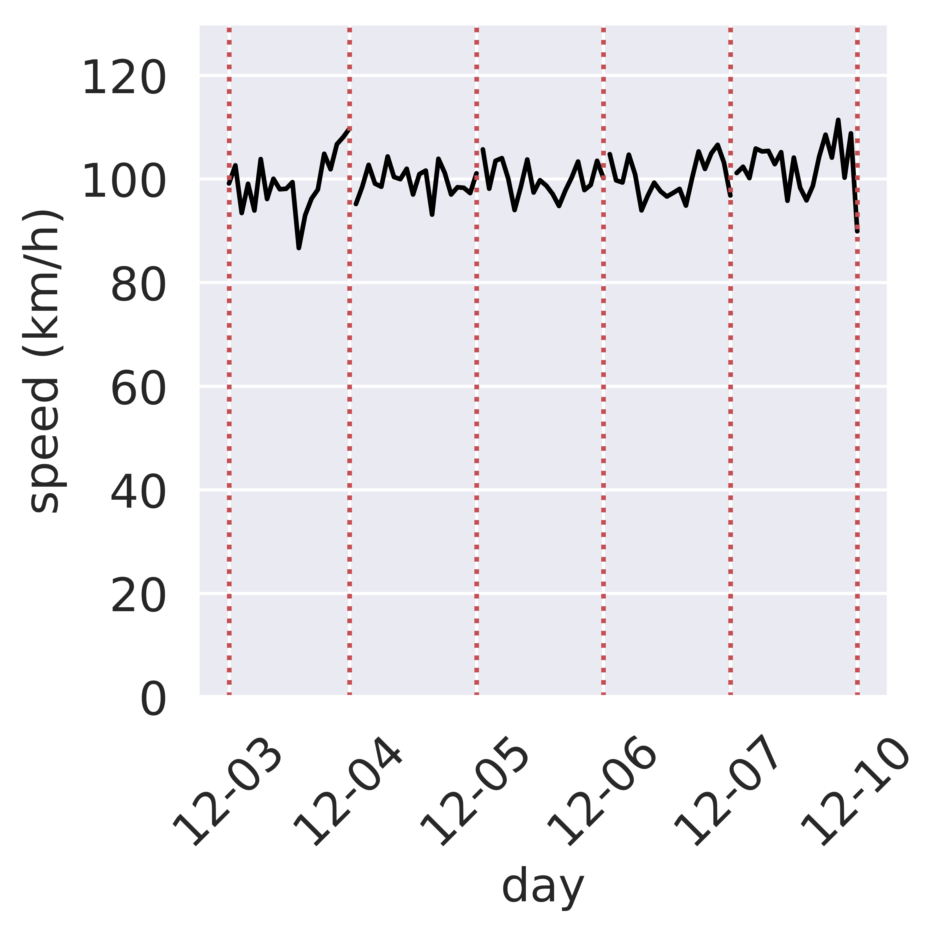
To demonstrate the practical interest of the proposal, the data used is concerned with the urban area of a French city, Rennes, made of n=144𝑛144n=144 days, p=556𝑝556p=556 road sections and T+1=20𝑇120T+1=20 time instants (from 333pm to 888pm) within each day (see Figure 1). Among all the considered methods, including the classical baseline from the time series analysis as well as the most recent neural network architecture, this is the regime switching model that yields the best performance.

The outline is as follows. In Section 2, the probabilistic framework is introduced. The optimal linear predictor is characterized, and the main assumptions are discussed. In Section 3, we present the main theoretical results of the paper that are bounds on the prediction error of (2). Section 4 investigates the regime switching variant. A comparative study including different methods applied to the real data presented before is proposed in Section 5. A simulation study is conducted in Section 6. All the proofs of the stated results are gathered in the Appendix.
Refer to caption
(a)
Refer to caption
(b)
Refer to caption
(c)
Refer to caption
(d)
Refer to caption
(e)
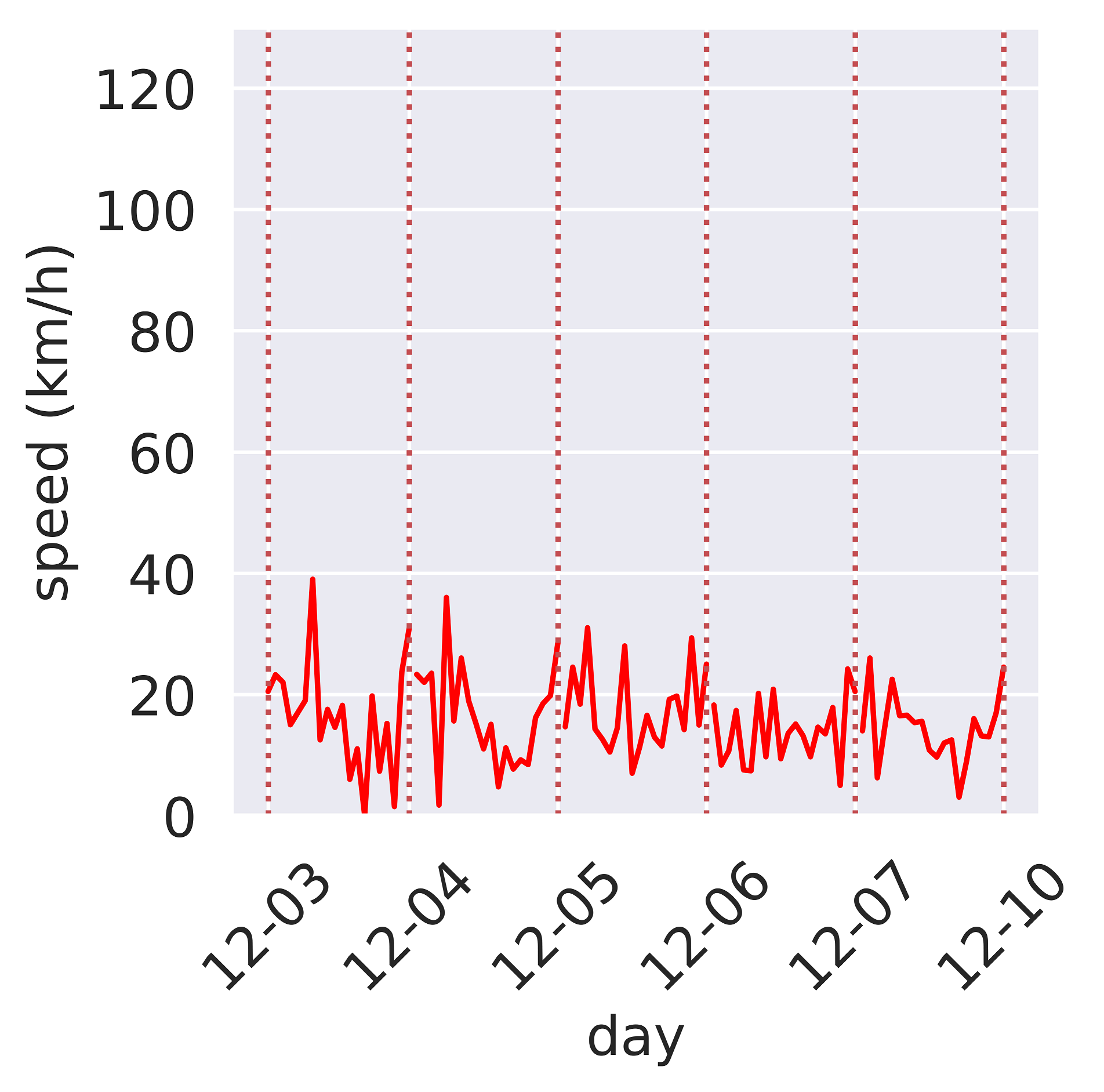
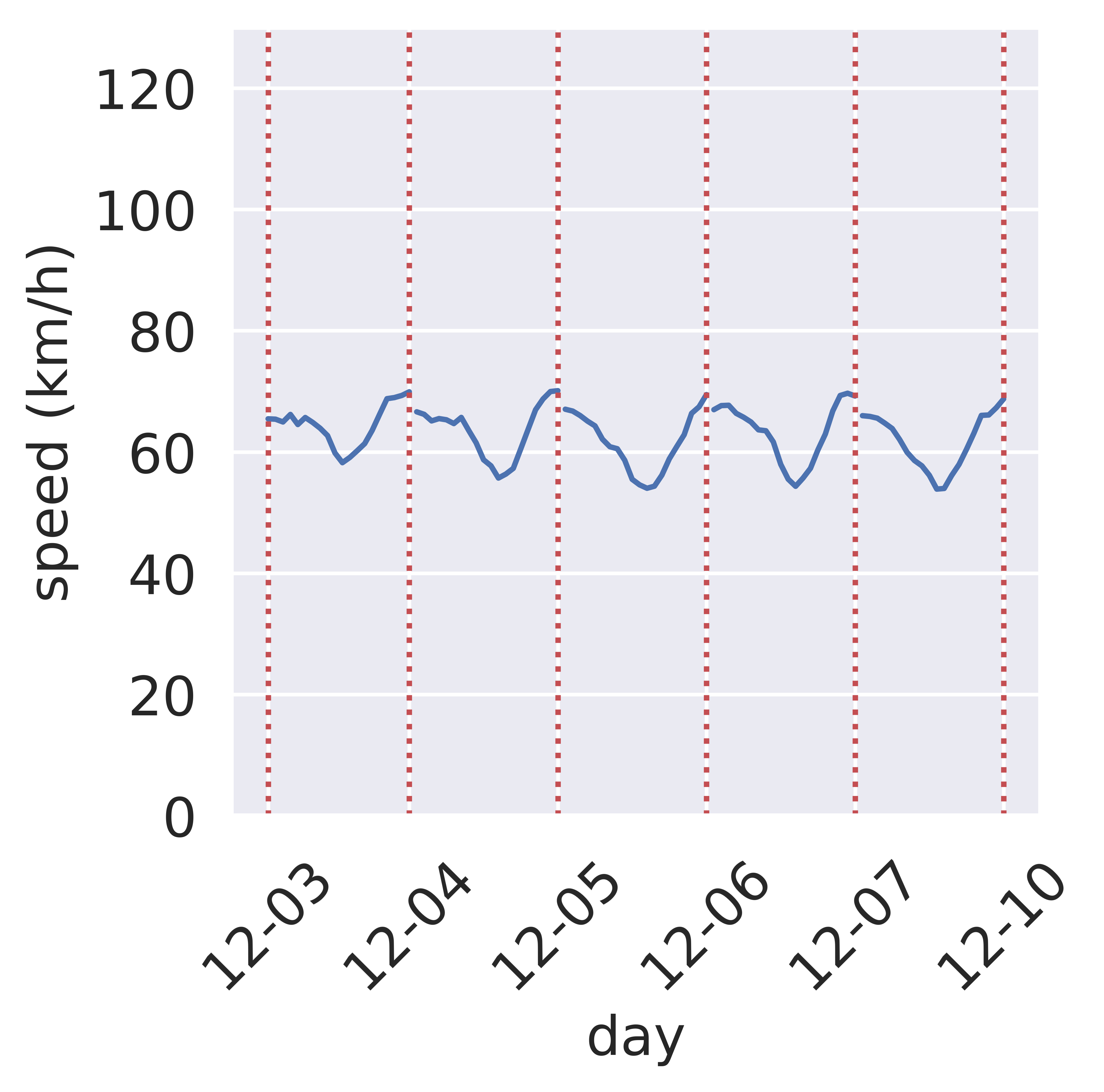
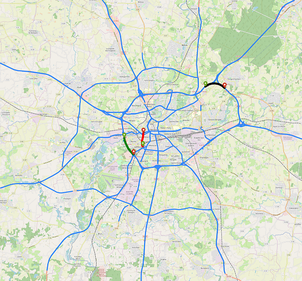
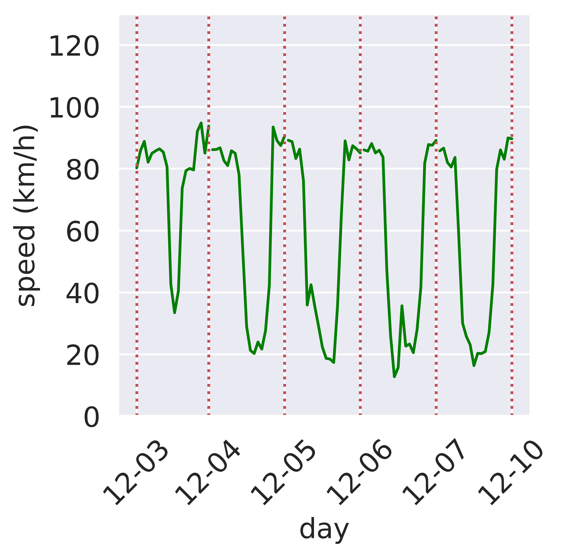
Figure 1: (a) Rennes road network is colored in blue and 333 representative sections are colored in green, black and red; (b) speeds observed during 666 days of December 201820182018 in the green section (cyclic behavior); (c) in the black section (high speed section); (d) in the red section (low speed section); (e) average speed over all sections in the road network during the same 666 days of December 201820182018.

2 Probabilistic framework

Let 𝒮={1,,p}𝒮1𝑝\mathcal{S}=\{1,\ldots,p\} denote an index set of p1𝑝1p\geqslant 1 real-valued variables that evolve during a time period 𝒯={0,,T}𝒯0𝑇\mathcal{T}=\{0,\ldots,T\}. These variables are gathered in a matrix of size p×(T+1)𝑝𝑇1p\times(T+1) denoted by W=(Wk,t)k𝒮,t𝒯𝑊subscriptsubscript𝑊𝑘𝑡formulae-sequence𝑘𝒮𝑡𝒯W=(W_{k,t})_{k\in\mathcal{S},\,t\in\mathcal{T}}. In road traffic data, k𝒮𝑘𝒮k\in\mathcal{S} stands for the section index of the road network 𝒮𝒮\mathcal{S}, t𝒯𝑡𝒯t\in\mathcal{T} for the time instants within the day, and Wk,tsubscript𝑊𝑘𝑡W_{k,t} is the speed recorded at section k𝑘k and time t𝑡t. We denote by W{,t}psubscript𝑊𝑡superscript𝑝W_{\{\cdot,t\}}\in\mathbb{R}^{p} the vector of speed at time t𝒯𝑡𝒯t\in\mathcal{T}. The following probabilistic framework will be adopted throughout the paper.

Assumption 1 (probabilistic framework).

Let (Ω,,P)Ω𝑃(\Omega,\mathcal{F},P) be a probability space. The matrix W=(W{,0},,W{,T})p×(T+1)𝑊subscript𝑊0subscript𝑊𝑇superscript𝑝𝑇1W=(W_{\{\cdot,0\}},\ldots,W_{\{\cdot,T\}})\in\mathbb{R}^{p\times(T+1)} is a random element valued in p×(T+1)superscript𝑝𝑇1\mathbb{R}^{p\times(T+1)} with distribution P𝑃P. For all k𝒮𝑘𝒮k\in\mathcal{S} and t𝒯𝑡𝒯t\in\mathcal{T}, we have E[Wk,t2]<+𝐸delimited-[]superscriptsubscript𝑊𝑘𝑡2E[W_{k,t}^{2}]<+\infty (E𝐸E stands for the expectation with respect to P𝑃P).

The task of interest is to predict the state variable at time t𝑡t, W{,t}subscript𝑊𝑡W_{\{\cdot,t\}}, using the information available at time t1𝑡1t-1, W{,t1}subscript𝑊𝑡1W_{\{\cdot,t-1\}}. The model at use to predict W{,t}subscript𝑊𝑡W_{\{\cdot,t\}} is given by the mapping L(W{,t1})=bt+AW{,t1}𝐿subscript𝑊𝑡1subscript𝑏𝑡𝐴subscript𝑊𝑡1L(W_{\{\cdot,t-1\}})=b_{t}+AW_{\{\cdot,t-1\}}, where Ap×p𝐴superscript𝑝𝑝A\in\mathbb{R}^{p\times p} and btpsubscript𝑏𝑡superscript𝑝b_{t}\in\mathbb{R}^{p} are parameters that shall be estimated. Define

Y=(W{,1},,W{,T})andX=(W{,0},,W{,T1}).formulae-sequence𝑌subscript𝑊1subscript𝑊𝑇and𝑋subscript𝑊0subscript𝑊𝑇1\displaystyle Y=(W_{\{\cdot,1\}},\ldots,W_{\{\cdot,T\}})\qquad\text{and}\qquad X=(W_{\{\cdot,0\}},\ldots,W_{\{\cdot,T-1\}}).

Equipped with this notation, the problem can be expressed as a simple matrix-regression problem with covariate Xp×T𝑋superscript𝑝𝑇X\in\mathbb{R}^{p\times T} and output Yp×T𝑌superscript𝑝𝑇Y\in\mathbb{R}^{p\times T}. In matrix notation, the model simply writes

={L(X)=b+AX:bp×T,Ap×p},conditional-set𝐿𝑋𝑏𝐴𝑋formulae-sequence𝑏superscript𝑝𝑇𝐴superscript𝑝𝑝\displaystyle\mathcal{L}=\{L(X)=b+AX\,:\,b\in\mathbb{R}^{p\times T},\,A\in\mathbb{R}^{p\times p}\}, (3)

with L(X{,1},,X{,T})=(L(X{,1}),,L(X{,T}))𝐿subscript𝑋1subscript𝑋𝑇𝐿subscript𝑋1𝐿subscript𝑋𝑇L(X_{\{\cdot,1\}},\ldots,X_{\{\cdot,T\}})=(L(X_{\{\cdot,1\}}),\ldots,L(X_{\{\cdot,T\}})). The number of parameters needed to describe a single element in \mathcal{L} is p(p+T)𝑝𝑝𝑇p(p+T). Because the matrix A𝐴A is fixed over the period 𝒯𝒯\mathcal{T}, this model reflects a certain structural belief on the dependency along time between the state variables W{,t}subscript𝑊𝑡W_{\{\cdot,t\}}. Each element in \mathcal{L} is defined by a baseline matrix bp×T𝑏superscript𝑝𝑇b\in\mathbb{R}^{p\times T} which carries out the average behavior in the whole network and a matrix Ap×p𝐴superscript𝑝𝑝A\in\mathbb{R}^{p\times p} which encodes for the influence between the different road sections. Alternative models are discussed at the end of the section. The accuracy of a given model L𝐿L\in{\mathcal{L}} is measured through the (normalized) L2(P)subscript𝐿2𝑃L_{2}(P)-risk given by

R(L)=p1E[YL(X)F2].𝑅𝐿superscript𝑝1𝐸delimited-[]superscriptsubscriptnorm𝑌𝐿𝑋𝐹2\displaystyle R(L)=p^{-1}E[\|Y-L(X)\|_{F}^{2}].

Note that, because of the factor 1/p1𝑝1/p, R(L)𝑅𝐿R(L) is just the averaged squared error of L𝐿L. Among the class \mathcal{L}, there is an optimal predictor characterized by the usual normal equations. This is the statement of the next proposition.

Proposition 1.

Suppose that Assumption 1 is fulfilled. There is a unique minimizer LargminLR(L)superscript𝐿subscriptargmin𝐿𝑅𝐿L^{\star}\in\operatorname{argmin}_{L\in\mathcal{L}}R(L). Moreover L=L𝐿superscript𝐿L=L^{\star} if and only if E[YL(X)]=0𝐸delimited-[]𝑌𝐿𝑋0E[Y-L(X)]=0 and E[(YL(X))XT]=0𝐸delimited-[]𝑌𝐿𝑋superscript𝑋𝑇0E[(Y-L(X))X^{T}]=0.

The following decomposition of the risk underlines the prediction loss associated to the predictor L𝐿L by comparing it with the best predictor Lsuperscript𝐿L^{\star} in \mathcal{L}. Define the excess risk by

(L)=R(L)R(L),L.formulae-sequence𝐿𝑅𝐿𝑅superscript𝐿𝐿\displaystyle\mathcal{E}(L)=R(L)-R(L^{\star}),\qquad L\in{\mathcal{L}}.
Proposition 2.

Suppose that Assumption 1 is fulfilled. It holds:

L,for-all𝐿\displaystyle\forall L\in{\mathcal{L}},\qquad (L)=p1E[L(X)L(X)F2].𝐿superscript𝑝1𝐸delimited-[]superscriptsubscriptnorm𝐿𝑋superscript𝐿𝑋𝐹2\displaystyle\mathcal{E}(L)=p^{-1}E[\|L(X)-L^{\star}(X)\|_{F}^{2}].

In what follows, bounds are established on the excess risk under a certain asymptotic regime where both n𝑛n and p:=pnassign𝑝subscript𝑝𝑛p:=p_{n} go to infinity whereas T𝑇T remains fixed. Though theoretic, this regime is of practical interest as it permits to analyze cases where the number of sections p𝑝p is relatively large (possibly greater than n𝑛n). This implies that the sequence of random variables of interest must be introduced as a triangular array. For each n1𝑛1n\geqslant 1, we observe n𝑛n realizations of W𝑊W: W(1),,W(n)superscript𝑊1superscript𝑊𝑛W^{(1)},\ldots,W^{(n)} where for each i𝑖i, W(i)p×(T+1)superscript𝑊𝑖superscript𝑝𝑇1W^{(i)}\in\mathbb{R}^{p\times(T+1)}. The following modeling assumption will be the basis to derive theoretical guarantees on (L)𝐿\mathcal{E}(L).

Assumption 2 (daily regeneration).

For each n1𝑛1n\geqslant 1, (W(i))1insubscriptsuperscript𝑊𝑖1𝑖𝑛(W^{(i)})_{1\leqslant i\leqslant n} is an independent and identically distributed collection of random variables defined on (Ω,,P)Ω𝑃(\Omega,\mathcal{F},P).

The daily regeneration assumption has two components: the independence between the days and the probability distribution of each day which stays the same. The independence is in accordance with the practical use of the road network where at night only a few people use the network so it can regenerate and hence “forgets” its past. The fact that each day has the same distribution means essentially that only days of similar types are gathered in the data. For instance, this assumption might not hold when mixing weekend days and workdays. This assumption also implies that the network structure remains unchanged during data collection.

Empirical check of the daily regeneration assumption

To check the daily regeneration assumption on the real data presented in the introduction, we extract a set of p(T+1)=11120𝑝𝑇111120p(T+1)=11120 one-dimensional time series. Each of these is associated to a specific instant in the day t𝑡t and a specific section k𝑘k, i.e., each time series is given by (Wk,t(i))i=1,,nsubscriptsuperscriptsubscript𝑊𝑘𝑡𝑖𝑖1𝑛(W_{k,t}^{(i)})_{i=1,\ldots,n} using the introduced notation. For each series, we run the test presented in Broock et al., (1996) where the null hypothesis is that the time series is independent and identically distributed. For most sections, 88%percent8888\%, the null hypothesis is not rejected at a nominal level of 95%percent9595\%. This clearly validates the daily regeneration assumption. The share of sections, 12%percent1212\%, for which the hypothesis has been rejected, can be explained by the presence of missing values in the data which have been replaced by the average value (see Section 5 for details). It is also likely that external events such as roadworks and constructions have impacted the result of the test.

Alternative models

Two alternative modeling approaches might have been considered at the price of additional notation and minor changes in the proofs of the results presented in the next section. The first alternative is obtained by imposing the matrix A𝐴A to be diagonal. In this case, each 111-dimensional vector coordinates is fitted using an auto-regressive model based on one single lag. The second alternative is to use more than one lag, say H1𝐻1H\geqslant 1, to predict the next coming instance. This is done by enlarging the matrix A𝐴A to (A1,,AH)subscript𝐴1subscript𝐴𝐻(A_{1},\ldots,A_{H}) where each Ahp×psubscript𝐴superscript𝑝𝑝A_{h}\in\mathbb{R}^{p\times p} and by stacking in X𝑋X the H𝐻H previous lags. These two variations, though interesting, are not presented in the paper for the sake of readability. Another approach which will be addressed in Section 4 is when the matrix A𝐴A is allowed to change across time.

3 Empirical risk minimization

3.1 Definitions and first results

Given a sequence (W(i))1inp×(T+1)subscriptsuperscript𝑊𝑖1𝑖𝑛superscript𝑝𝑇1(W^{(i)})_{1\leqslant i\leqslant n}\subset\mathbb{R}^{p\times(T+1)} and a regularization parameter λ0𝜆0\lambda\geqslant 0, define the estimate

(b^,A^)argminbp×T,Ap×p(i=1nY(i)bAX(i)F2)+2λA1,^𝑏^𝐴subscriptargminformulae-sequence𝑏superscript𝑝𝑇𝐴superscript𝑝𝑝superscriptsubscript𝑖1𝑛superscriptsubscriptnormsuperscript𝑌𝑖𝑏𝐴superscript𝑋𝑖𝐹22𝜆subscriptnorm𝐴1\displaystyle(\hat{b},\hat{A})\in\operatorname{argmin}_{b\in\mathbb{R}^{p\times T},\,A\in\mathbb{R}^{p\times p}}\left(\sum_{i=1}^{n}\|Y^{(i)}-b-AX^{(i)}\|_{F}^{2}\right)+2\lambda\|A\|_{1}, (4)

with

Y(i)=(W{,1}(i),,W{,T}(i))andX(i)=(W{,0}(i),,W{,T1}(i)).formulae-sequencesuperscript𝑌𝑖superscriptsubscript𝑊1𝑖superscriptsubscript𝑊𝑇𝑖andsuperscript𝑋𝑖superscriptsubscript𝑊0𝑖superscriptsubscript𝑊𝑇1𝑖\displaystyle Y^{(i)}=(W_{\{\cdot,1\}}^{(i)},\ldots,W_{\{\cdot,T\}}^{(i)})\qquad\text{and}\qquad X^{(i)}=(W_{\{\cdot,0\}}^{(i)},\ldots,W_{\{\cdot,T-1\}}^{(i)}).

For any vector up𝑢superscript𝑝u\in\mathbb{R}^{p} and any integer q1𝑞1q\geqslant 1, the qsubscript𝑞\ell_{q}-norm is defined as uqq=k=1p|uk|qsuperscriptsubscriptnorm𝑢𝑞𝑞superscriptsubscript𝑘1𝑝superscriptsubscript𝑢𝑘𝑞\|u\|_{q}^{q}=\sum_{k=1}^{p}|u_{k}|^{q}. The prediction at point Xp×T𝑋superscript𝑝𝑇X\in\mathbb{R}^{p\times T} is given by

L^(X)=b^+A^X.^𝐿𝑋^𝑏^𝐴𝑋\hat{L}(X)=\hat{b}+\hat{A}X.

As the intercept in classical regression, the matrix parameter b^^𝑏\hat{b} is only a centering term. Indeed, when minimizing (4) with respect to b𝑏b only, we find b=n1i=1n{Y(i)AX(i)}𝑏superscript𝑛1superscriptsubscript𝑖1𝑛superscript𝑌𝑖𝐴superscript𝑋𝑖b=n^{-1}\sum_{i=1}^{n}\{Y^{(i)}-AX^{(i)}\}. The value of A^^𝐴\hat{A} can thus be obtained by solving the least-squares problem (4) without intercept and with empirically centered variables. Given A^^𝐴\hat{A}, the matrix b^^𝑏\hat{b} can be recovered using the simple formula b^=n1i=1n{Y(i)A^X(i)}^𝑏superscript𝑛1superscriptsubscript𝑖1𝑛superscript𝑌𝑖^𝐴superscript𝑋𝑖\hat{b}=n^{-1}\sum_{i=1}^{n}\{Y^{(i)}-\hat{A}X^{(i)}\}. Consequently, the prediction at point X𝑋X may be written as L^(X)=Y¯n+A^(XX¯n)^𝐿𝑋superscript¯𝑌𝑛^𝐴𝑋superscript¯𝑋𝑛\hat{L}(X)=\overline{Y}^{n}+\hat{A}(X-\overline{X}^{n}), where, generically, M¯n=n1i=1nM(i)superscript¯𝑀𝑛superscript𝑛1superscriptsubscript𝑖1𝑛superscript𝑀𝑖\overline{M}^{n}=n^{-1}\sum_{i=1}^{n}M^{(i)}. Similarly, one has L(X)=E[Y]+A(XE(X))superscript𝐿𝑋𝐸delimited-[]𝑌superscript𝐴𝑋𝐸𝑋L^{\star}(X)=E[Y]+A^{\star}(X-E(X)). The previous two expressions emphasize that the excess risk might be decomposed according to 222 terms: one is dealing with the estimation error on Asuperscript𝐴A^{\star} and one is relative to the error on the averages E[Y]𝐸delimited-[]𝑌E[Y] and E[X]𝐸delimited-[]𝑋E[X]. We now state this decomposition.

Proposition 3.

Suppose that Assumption 1 is fulfilled. It holds that

(L^)^𝐿\displaystyle\mathcal{E}(\hat{L}) p1{(AA^)Σ1/2F2+2E(Y)Y¯nF2+2A^(E(X)X¯n)F2}.absentsuperscript𝑝1superscriptsubscriptnormsuperscript𝐴^𝐴superscriptΣ12𝐹22superscriptsubscriptnorm𝐸𝑌superscript¯𝑌𝑛𝐹22superscriptsubscriptnorm^𝐴𝐸𝑋superscript¯𝑋𝑛𝐹2\displaystyle\leqslant p^{-1}\{\|(A^{\star}-\hat{A})\Sigma^{1/2}\|_{F}^{2}+2\|E(Y)-\overline{Y}^{n}\|_{F}^{2}+2\|\hat{A}(E(X)-\overline{X}^{n})\|_{F}^{2}\}.

where Σ=E[(XE(X))(XE(X))T]Σ𝐸delimited-[]𝑋𝐸𝑋superscript𝑋𝐸𝑋𝑇\Sigma=E[(X-E(X))(X-E(X))^{T}].

The previous proposition will be the key to control the excess risk of both the OLS and LASSO predictors. The OLS (resp. LASSO) estimate, which results from (4) when λ=0𝜆0\lambda=0 (resp. λ>0𝜆0\lambda>0), is denoted by (b^(ols),A^(ols))superscript^𝑏𝑜𝑙𝑠superscript^𝐴𝑜𝑙𝑠(\hat{b}^{(ols)},\,\hat{A}^{(ols)}) (resp. (b^(lasso),A^(lasso))superscript^𝑏𝑙𝑎𝑠𝑠𝑜superscript^𝐴𝑙𝑎𝑠𝑠𝑜(\hat{b}^{(lasso)},\,\hat{A}^{(lasso)})) and its associated predictor is given by L^(ols)superscript^𝐿𝑜𝑙𝑠\hat{L}^{(ols)} (resp. L^(lasso)superscript^𝐿𝑙𝑎𝑠𝑠𝑜\hat{L}^{(lasso)}).

3.2 Ordinary least-squares

In this section, we study the case of the OLS (i.e., when λ=0𝜆0\lambda=0). This will allow to put into perspective the main results of the paper, concerning the LASSO (i.e., when λ>0𝜆0\lambda>0), that will be given in the next section. We now introduce certain assumptions dealing with the distribution of W(i)superscript𝑊𝑖W^{(i)}, which depends on n𝑛n trough p=pn𝑝subscript𝑝𝑛p=p_{n}. The following one claims that the covariates are uniformly bounded.

Assumption 3 (bounded variables).

With probability 111,

lim supnmaxk𝒮,t𝒯|Xk,t|<.subscriptlimit-supremum𝑛subscriptformulae-sequence𝑘𝒮𝑡𝒯subscript𝑋𝑘𝑡\limsup_{n\to\infty}\max_{k\in\mathcal{S},\,t\in\mathcal{T}}|X_{k,t}|<~{}\infty.

The following invertibility condition on ΣΣ\Sigma can be seen as an identification condition since the matrix Asuperscript𝐴A^{\star} is unique under this hypothesis. Denote by γ>0𝛾0\gamma>0 the smallest eigenvalue of ΣΣ\Sigma.

Assumption 4.

lim infnγ>0subscriptlimit-infimum𝑛𝛾0\liminf_{n\to\infty}\gamma>0 .

Finally, introduce the noise level σ2>0superscript𝜎20\sigma^{2}>0 which consists in a bound on the conditional variance of the residual matrix

ϵ={YL(X)},italic-ϵ𝑌superscript𝐿𝑋\displaystyle\epsilon=\{Y-L^{\star}(X)\},

given the covariates X𝑋X. Formally, σ2superscript𝜎2\sigma^{2} is the smallest positive real number such that, with probability 111, maxk𝒮,t𝒯E[ϵk,t2|X{,t}]σ2subscriptformulae-sequence𝑘𝒮𝑡𝒯𝐸delimited-[]conditionalsuperscriptsubscriptitalic-ϵ𝑘𝑡2subscript𝑋𝑡superscript𝜎2\max_{k\in\mathcal{S},\,t\in\mathcal{T}}E[\epsilon_{k,t}^{2}|X_{\{\cdot,t\}}]\leqslant\sigma^{2}. Note that σ2superscript𝜎2\sigma^{2} might depend on p𝑝p. The fact that it does not depend on X𝑋X stresses the homoscedasticity of the regression model.

Assumption 5.

lim infnσ>0subscriptlimit-infimum𝑛𝜎0\liminf_{n\to\infty}\sigma>0.

We stress that both previous assumptions on γ𝛾\gamma and σ𝜎\sigma might be alleviated at the price of additional technical assumptions which might be deduced from our proofs. The following result provides a bound on the excess risk associated to the OLS procedure. The given bound depends explicitly on the quantities of interest n𝑛n and p𝑝p as well as on the underlying probabilistic model through Asuperscript𝐴A^{\star}. The asymptotic framework we consider is with respect to n𝑛n\to\infty and we allow the dimension p𝑝p to go to infinity (with a certain restriction). A discussion is provided below the proposition.

Proposition 4.

Suppose that Assumptions 1, 2, 3, 4 and 5 are fulfilled. Suppose that n𝑛n\to\infty and p=pn𝑝subscript𝑝𝑛p=p_{n}\to\infty such that plog(p)/n0𝑝𝑝𝑛0p\log(p)/n\to 0, we have

(L^(ols))=OP(pσ2+AF2/pn).superscript^𝐿𝑜𝑙𝑠subscript𝑂𝑃𝑝superscript𝜎2superscriptsubscriptnormsuperscript𝐴𝐹2𝑝𝑛\displaystyle\mathcal{E}(\hat{L}^{(ols)})=O_{P}\left({\frac{p\sigma^{2}+\|A^{\star}\|_{F}^{2}/p}{n}}\right).

The previous bound on the excess risk is badly affected by the parameter p𝑝p. First of all, the condition plog(p)/n0𝑝𝑝𝑛0p\log(p)/n\to 0 implies that pnmuch-less-than𝑝𝑛p\ll n. Second, the number of nonzero coefficients in A𝐴A poorly influences the bound. When A=Isuperscript𝐴𝐼A^{\star}=I, the second term equals 1/n1𝑛1/n and becomes negligible with respect to p/n𝑝𝑛p/n. In contrast, when A=(1)k,superscript𝐴subscript1𝑘A^{\star}=(1)_{k,\ell}, i.e., all the covariates are used to predict each output, it equals p/n𝑝𝑛p/n and becomes a leading term. In between, we have the situation where each line of Asuperscript𝐴A^{\star} possesses only a few non-zero coefficients. Then the magnitude of this term becomes 1/n1𝑛1/n. In this last case, some benefits are obtained when using the LASSO (λ>0𝜆0\lambda>0) instead of the OLS (λ=0𝜆0\lambda=0) as detailed in the next section.

3.3 Regularized least-squares

The LASSO approach is introduced to overcome the “large p𝑝p small n𝑛n” difficulties of the OLS previously discussed. In contrast with the OLS, the additional 1\|\cdot\|_{1}-penalty term shall enforce the estimated matrix A^(lasso)superscript^𝐴𝑙𝑎𝑠𝑠𝑜\hat{A}^{(lasso)} to be “sparse”, i.e., to have only a few non-zero coefficients. From a theoretical perspective, this will permit to take advantage of any sparsity structure in the matrix Asuperscript𝐴A^{\star} associated to Lsuperscript𝐿L^{\star}.

Introduce the active set Sksubscriptsuperscript𝑆𝑘S^{\star}_{k} as the set of non-zero coefficients of the k𝑘k-th line of Asuperscript𝐴A^{\star}, i.e., for each k𝒮𝑘𝒮k\in\mathcal{S},

Sk={𝒮:Ak,0}.subscriptsuperscript𝑆𝑘conditional-set𝒮superscriptsubscript𝐴𝑘0\displaystyle S^{\star}_{k}=\left\{\ell\in\mathcal{S}\quad:\quad A_{k,\ell}^{\star}\neq 0\right\}.

As stated in the following assumption, the sparsity level of each line of Asuperscript𝐴A^{\star} is assumed to be bounded uniformly over n𝑛n.

Assumption 6.

lim supnmaxk𝒮|Sk|<subscriptlimit-supremum𝑛subscript𝑘𝒮superscriptsubscript𝑆𝑘\limsup_{n\to\infty}\max_{k\in\mathcal{S}}|S_{k}^{\star}|<\infty.

The following assumption is a relaxation of Assumption 4 which was needed in the study of the OLS approach. For any set S𝒮𝑆𝒮S\subset\mathcal{S}, denote by Scsuperscript𝑆𝑐S^{c} its complement in 𝒮𝒮\mathcal{S}, and introduce the cone

𝒞(S,α)={up:uSc1αuS1}.𝒞𝑆𝛼conditional-set𝑢superscript𝑝subscriptnormsubscript𝑢superscript𝑆𝑐1𝛼subscriptnormsubscript𝑢𝑆1\displaystyle\mathcal{C}(S,\alpha)=\{u\in\mathbb{R}^{p}\,:\,\|u_{S^{c}}\|_{1}\leqslant\alpha\|u_{S}\|_{1}\}.

Denote by γsuperscript𝛾\gamma^{\star} the smallest nonnegative number such that for all k𝒮𝑘𝒮k\in\mathcal{S}, we have Σ1/2u22γu22superscriptsubscriptnormsuperscriptΣ12𝑢22superscript𝛾superscriptsubscriptnorm𝑢22\|\Sigma^{1/2}u\|_{2}^{2}\geqslant\gamma^{\star}\|u\|_{2}^{2}, u𝒞(Sk,3)for-all𝑢𝒞superscriptsubscript𝑆𝑘3\forall u\in\mathcal{C}(S_{k}^{\star},3).

Assumption 7.

lim infnγ>0subscriptlimit-infimum𝑛superscript𝛾0\liminf_{n\to\infty}\gamma^{\star}>0.

Similar to Assumption 4, the previous assumption can be alleviated by allowing the value γsuperscript𝛾\gamma^{\star} to go to 00 at a certain rate which can be deduced from our proof. We are now in position to give an upper bound on the excess risk for the LASSO model.

Proposition 5.

Suppose that Assumptions 1, 2, 3, 5, 6 and 7 are fulfilled. Suppose that n𝑛n\to\infty and p=pn𝑝subscript𝑝𝑛p=p_{n}\to\infty such that log(p)/n0𝑝𝑛0\log(p)/n\to 0, we have

(L^(lasso))=OP(log(p)n).superscript^𝐿𝑙𝑎𝑠𝑠𝑜subscript𝑂𝑃𝑝𝑛\displaystyle\mathcal{E}(\hat{L}^{(lasso)})=O_{P}\left({\frac{\log(p)}{n}}\right).

provided that λ=Cnσ2log(p)𝜆𝐶𝑛superscript𝜎2𝑝\lambda=C\sqrt{n\sigma^{2}\log(p)}, for some constant C>0𝐶0C>0.

The parameter p𝑝p which influenced badly the bound obtained on the OLS excess risk is here replaced by log(p)𝑝\log(p). This shows that without any knowledge on the active variables, the LASSO approach enables to recover the accuracy (at the price of a logarithmic factor) of an “oracle” OLS estimator that would use only the active variables. Another notable advantage is that the assumptions for the validity of the bound have been reduced to log(p)/n0𝑝𝑛0\log(p)/n\to 0 compared to the OLS which needed plog(p)/n0𝑝𝑝𝑛0p\log(p)/n\to 0.

The LASSO requires to choose the regularization parameter λ𝜆\lambda which controls the number of selected covariates. In the proof, we follow the classic approach (as presented in Hastie et al., (2015)) by choosing λ𝜆\lambda as small as possible but larger than a certain empirical sum involving the residuals of the model; see (11) in the Appendix. This explains our choice λ=Cnσ2log(p)𝜆𝐶𝑛superscript𝜎2𝑝\lambda=C\sqrt{n\sigma^{2}\log(p)}. Note that we could have done differently. Since the Frobenius norm writes as the sum of the 2subscript2\ell_{2}-norms of the matrix lines, problem (4) can be expressed trough p𝑝p standard LASSO sub-problems each having T𝑇T outputs. This allows to select different values of λ𝜆\lambda in each sub-problem. In practice, λ𝜆\lambda will be chosen using cross-validation as explained in the simulation section.

4 Regime switching

Regime switching occurs when the distribution of road traffic changes after a certain time t{1,,T}superscript𝑡1𝑇t^{*}\in\{1,\ldots,T\}. For instance, it might happen that a certain matrix Asuperscript𝐴A^{\star} is suitable to model the morning traffic while another matrix is needed to fit conveniently the afternoon behavior. To account for these potential changes in the distribution, we consider a wider predictive model than the one presented in Section 2. The set of predictors to be considered here writes as t=1,,Ttsubscript𝑡1𝑇subscript𝑡\cup_{t=1,\ldots,T}\mathcal{L}_{t} where each tsubscript𝑡\mathcal{L}_{t} is given by

{b+(AX1,,AXt,AXt+1,AXT):bp×T,Ap×p,Ap×p}.conditional-set𝑏𝐴subscript𝑋1𝐴subscript𝑋𝑡superscript𝐴subscript𝑋𝑡1superscript𝐴subscript𝑋𝑇formulae-sequence𝑏superscript𝑝𝑇formulae-sequence𝐴superscript𝑝𝑝superscript𝐴superscript𝑝𝑝\displaystyle\{b+(AX_{1},\ldots,AX_{t},A^{\prime}X_{t+1}\ldots,A^{\prime}X_{T})\,:\,b\in\mathbb{R}^{p\times T},A\in\mathbb{R}^{p\times p},\,A^{\prime}\in\mathbb{R}^{p\times p}\}.

Each submodel tsubscript𝑡\mathcal{L}_{t} corresponds to a regime switching occurring at time t𝑡t. Note that the case t=T𝑡𝑇t=T corresponds to the model without regime switching, i.e., a single matrix A𝐴A is used for the whole day. Within each submodel, the optimal predictor is defined as

Lt=argminLtR(L),subscriptsuperscript𝐿𝑡subscriptargmin𝐿subscript𝑡𝑅𝐿\displaystyle L^{\star}_{t}=\operatorname{argmin}_{L\in{\mathcal{L}_{t}}}R(L),

and satisfies some normal equations (involving A𝐴A and Asuperscript𝐴A^{\prime}) that can be recovered by applying Proposition 1 with a specific range for 𝒯𝒯\mathcal{T}. The risk associated to a submodel t𝑡t is then given by R(Lt)𝑅subscriptsuperscript𝐿𝑡R(L^{\star}_{t}).

If the change point tsuperscript𝑡t^{\star} where given, then the situation would be very similar to what has been studied in the previous section except that two predictors would need to be estimated, one for each time range U={1,,t}superscript𝑈1superscript𝑡U^{\star}=\{1,\ldots,t^{\star}\} and V={t+1,,T}superscript𝑉superscript𝑡1𝑇V^{*}=\{t^{\star}+1,\ldots,T\}. As each predictor would be computed as

(b^t,A^t)argminbp×t,Ap×pi=1nY{,U}(i)bAX{,U}(i)F2+2λA1,subscript^𝑏superscript𝑡subscript^𝐴superscript𝑡subscriptargminformulae-sequence𝑏superscript𝑝superscript𝑡𝐴superscript𝑝𝑝superscriptsubscript𝑖1𝑛superscriptsubscriptnormsuperscriptsubscript𝑌superscript𝑈𝑖𝑏𝐴superscriptsubscript𝑋superscript𝑈𝑖𝐹22𝜆subscriptnorm𝐴1\displaystyle(\hat{b}_{t^{\star}},\hat{A}_{t^{\star}})\in\operatorname{argmin}_{b\in\mathbb{R}^{p\times t^{\star}},\,A\in\mathbb{R}^{p\times p}}\sum_{i=1}^{n}\|Y_{\{\cdot,U^{\star}\}}^{(i)}-b-AX_{\{\cdot,U^{\star}\}}^{(i)}\|_{F}^{2}+2\lambda\|A\|_{1},
(b^t,A^t)argminbp×(Tt),Ap×pi=1nY{,V}(i)bAX{,V}(i)F2+2λA1,superscriptsubscript^𝑏superscript𝑡superscriptsubscript^𝐴superscript𝑡subscriptargminformulae-sequence𝑏superscript𝑝𝑇superscript𝑡𝐴superscript𝑝𝑝superscriptsubscript𝑖1𝑛superscriptsubscriptnormsuperscriptsubscript𝑌superscript𝑉𝑖𝑏𝐴superscriptsubscript𝑋superscript𝑉𝑖𝐹22𝜆subscriptnorm𝐴1\displaystyle(\hat{b}_{t^{\star}}^{\prime},\hat{A}_{t^{\star}}^{\prime})\in\operatorname{argmin}_{b\in\mathbb{R}^{p\times(T-t^{\star})},\,A\in\mathbb{R}^{p\times p}}\sum_{i=1}^{n}\|Y_{\{\cdot,V^{\star}\}}^{(i)}-b-AX_{\{\cdot,{V^{\star}}\}}^{(i)}\|_{F}^{2}+2\lambda\|A\|_{1},

the results obtained in the previous section would apply to both estimates separately and one would easily derive an excess risk bound when the change point tsuperscript𝑡t^{\star} is known. The key point here is thus to recover the change point tsuperscript𝑡t^{*} by some procedure. Next, we study a model selection approach based on cross-validation to estimate tsuperscript𝑡t^{\star}.

Suppose that T2𝑇2T\geqslant 2. For each t{1,,T}𝑡1𝑇t\in\{1,\ldots,T\}, define Ut={1,,t}subscript𝑈𝑡1𝑡U_{t}=\{1,\ldots,t\}, Vt={t+1,,T}subscript𝑉𝑡𝑡1𝑇{V_{t}}=\{t+1,\ldots,T\} and let ={I1,,IK}subscript𝐼1subscript𝐼𝐾\mathcal{F}=\{I_{1},\ldots,I_{K}\} be a partition of {1,,n}1𝑛\{1,\ldots,n\} whose elements Iksubscript𝐼𝑘I_{k} are called folds. We suppose further that each fold contains the same number of observation n/K𝑛𝐾n/K. For each fold I𝐼I\in\mathcal{F}, define

(b^J,t,A^J,t)argminbp×t,Ap×piJY{,Ut}(i)bAX{,Ut}(i)F2+2λA1,subscript^𝑏𝐽𝑡subscript^𝐴𝐽𝑡subscriptargminformulae-sequence𝑏superscript𝑝𝑡𝐴superscript𝑝𝑝subscript𝑖𝐽superscriptsubscriptnormsuperscriptsubscript𝑌subscript𝑈𝑡𝑖𝑏𝐴superscriptsubscript𝑋subscript𝑈𝑡𝑖𝐹22𝜆subscriptnorm𝐴1\displaystyle(\hat{b}_{J,t},\hat{A}_{J,t})\in\operatorname{argmin}_{b\in\mathbb{R}^{p\times t},\,A\in\mathbb{R}^{p\times p}}\sum_{i\in J}\|Y_{\{\cdot,U_{t}\}}^{(i)}-b-AX_{\{\cdot,U_{t}\}}^{(i)}\|_{F}^{2}+2\lambda\|A\|_{1},
(b^J,t,A^J,t)argminbp×(Tt),Ap×piJY{,Vt}(i)bAX{,Vt}(i)F2+2λA1,superscriptsubscript^𝑏𝐽𝑡superscriptsubscript^𝐴𝐽𝑡subscriptargminformulae-sequence𝑏superscript𝑝𝑇𝑡𝐴superscript𝑝𝑝subscript𝑖𝐽superscriptsubscriptnormsuperscriptsubscript𝑌subscript𝑉𝑡𝑖𝑏𝐴superscriptsubscript𝑋subscript𝑉𝑡𝑖𝐹22𝜆subscriptnorm𝐴1\displaystyle(\hat{b}_{J,t}^{\prime},\hat{A}_{J,t}^{\prime})\in\operatorname{argmin}_{b\in\mathbb{R}^{p\times(T-t)},\,A\in\mathbb{R}^{p\times p}}\sum_{i\in J}\|Y_{\{\cdot,{V_{t}}\}}^{(i)}-b-AX_{\{\cdot,{V_{t}}\}}^{(i)}\|_{F}^{2}+2\lambda\|A\|_{1},

where J𝐽J is the complement of I𝐼I in {1,,n}1𝑛\{1,\ldots,n\}. To lighten the notations, the superscript (Lasso)𝐿𝑎𝑠𝑠𝑜(Lasso) will be from now on avoided. The estimate of the risk based on the fold I𝐼I is defined as

R^I,t=KnpiI{Y{,Ut}(i)b^J,tA^J,tX{,Ut}(i)F2+Y{,Vt}(i)b^J,tA^J,tX{,Vt}(i)F2}.subscript^𝑅𝐼𝑡𝐾𝑛𝑝subscript𝑖𝐼superscriptsubscriptnormsuperscriptsubscript𝑌subscript𝑈𝑡𝑖subscript^𝑏𝐽𝑡subscript^𝐴𝐽𝑡superscriptsubscript𝑋subscript𝑈𝑡𝑖𝐹2superscriptsubscriptnormsuperscriptsubscript𝑌subscript𝑉𝑡𝑖superscriptsubscript^𝑏𝐽𝑡superscriptsubscript^𝐴𝐽𝑡superscriptsubscript𝑋subscript𝑉𝑡𝑖𝐹2\displaystyle\hat{R}_{I,t}=\frac{K}{np}\sum_{i\in I}\{\|Y_{\{\cdot,U_{t}\}}^{(i)}-\hat{b}_{J,t}-\hat{A}_{J,t}X_{\{\cdot,U_{t}\}}^{(i)}\|_{F}^{2}+\|Y_{\{\cdot,V_{t}\}}^{(i)}-\hat{b}_{J,t}^{\prime}-\hat{A}_{J,t}^{\prime}X_{\{\cdot,V_{t}\}}^{(i)}\|_{F}^{2}\}.

The resulting cross-validation estimate of Rtsubscript𝑅𝑡R_{t} is then the average over the folds I𝐼I\in\mathcal{F} of the risks R^I,tsubscript^𝑅𝐼𝑡\hat{R}_{I,t} and the estimated change point t^^𝑡\hat{t} is the one having the smallest estimated risk, i.e.,

t^argmint=1,,TR^t:=1KIR^I,t.^𝑡subscriptargmin𝑡1𝑇subscript^𝑅𝑡assign1𝐾subscript𝐼subscript^𝑅𝐼𝑡\displaystyle\hat{t}\in\operatorname{argmin}_{t=1,\ldots,T}\hat{R}_{t}:=\frac{1}{K}\sum_{I\in\mathcal{F}}\hat{R}_{I,t}.

This t^^𝑡\hat{t} represents the best instant from which a different (linear) model shall be used. The following proposition provides a rate of convergence for the cross-validation risk estimate.

Proposition 6.

Under the assumptions of Proposition 5, we have for all t{1,T1}𝑡1𝑇1t\in\{1,\ldots T-1\},

|R^tR(Lt)|=OP(log(p)n).subscript^𝑅𝑡𝑅subscriptsuperscript𝐿𝑡subscript𝑂𝑃𝑝𝑛\displaystyle|\hat{R}_{t}-R(L^{\star}_{t})|=O_{P}\left(\sqrt{\frac{\log(p)}{n}}\right).

The difficulty in proving the previous result is to suitably control for the large dimension in the decomposition of the error. This is done by relying on a bound on the 1subscript1\ell_{1}-error associated to the matrix estimate A^n(lasso)superscriptsubscript^𝐴𝑛𝑙𝑎𝑠𝑠𝑜\hat{A}_{n}^{(lasso)}; see Proposition 7 in the Appendix.

Applying the previous proposition allows to establish the consistency of the cross-validation detection procedure.

Corollary 1.

Under the assumptions of Proposition 5, suppose there exists t{1,T1}superscript𝑡1𝑇1t^{*}\in\{1,\ldots T-1\} such that lim supnR(Lt)<lim infnR(Lt)subscriptlimit-supremum𝑛𝑅subscriptsuperscript𝐿superscript𝑡subscriptlimit-infimum𝑛𝑅subscriptsuperscript𝐿𝑡\limsup_{n\to\infty}R(L^{\star}_{t^{\star}})<\liminf_{n\to\infty}R(L^{\star}_{t}) for all tt𝑡superscript𝑡t\neq t^{*}, then

P(t^=t)1.𝑃^𝑡superscript𝑡1P(\hat{t}=t^{*})\to 1.

Interestingly, the previous regime switching detection can be iterated in a greedy procedure in which, at each step, we decide (based on cross-validation) if a regime switching is beneficial. If it does, we continue. If it does not, we stop. The study of such an iterative algorithm represents an interesting avenue for further research.

5 Real data analysis

This section provides a comparative study of different methods. First, real world data is presented followed by the different methods in competition and an analysis of the obtained results. Finally, graphical interpretations of the proposed LASSO approach are provided. A GitHub repository is available111https://github.com/mohammedLamine/RS-Lasso.

5.1 Dataset

The initial dataset contains the speed (km/h) and the location of each car using the Coyote navigation system (Floating car data). Data was collected in the Rennes road network from December 1, 2018 until July 9, 201920192019 every 303030 seconds. Signals were received from 113577113577113577 vehicle.

Some pre-processing is carried out to correct sensor errors and structure the data in a convenient format. First, the received locations are GPS coordinates whereas the model introduced here is based on the road section. Accordingly, we map-match the locations to the OpenStreetMap road network dataset (Greenfeld, , 2002) in order to obtain the section of each car location data. Second, to obtain data representing the flow in the sections of the network, we aggregate and average the observed speed values of cars over 151515-minute intervals for each section. Third, for some sections and time intervals, no value is observed. We therefore impute these values using the historical average associated to the time intervals and sections. To lower the number of missing values, we focus on a particularly busy time period from 333pm to 888pm (local time) of each workday. It is worth noting that this dataset comes from a low-frequency collection, meaning that for a given time and section, the average number of observations on the selected sections of the network is about 666 logs per 151515-minutes per section. This is due to the fact that we only observe a portion of the vehicles in the network (those equipped with Coyote GPS devices), and that suburban sections have low traffic. Thus, aiming for even higher precision (less than 151515 minutes) would increase the number of missing values.

In summary, we consider only the 151515-minute time intervals in the period from 333pm to 888pm (local time) of each workday only. The resulting dataset corresponds to our W(i)superscript𝑊𝑖W^{(i)}, i=1,,n𝑖1𝑛i=1,\ldots,n, matrices where p=556𝑝556p=556, n=144𝑛144n=144 and T+1=20𝑇120T+1=20 (Figure 1). We divide the data into 333 subsets: train 636363% (171017101710 examples), validation 272727% (741741741 examples), test 101010% (285285285 examples), splits are made such that days are not cut in the middle and all subsets contains sequential full days data.

5.2 Comparative study

5.2.1 Methods

The methods used in this study can be divided into two groups reflecting the information that is used to predict future values. In the first group, baselines are used to predict the speed using only data from the same section. The second group uses data collected from the entire network. This includes the linear predictors that have been previously studied and also certain neural network predictors that we introduce for the sake of completeness.

Baselines

  • Historical average (HA): for each section k𝑘k and time interval t𝑡t, the prediction is given by the average speed at time interval t𝑡t and section k𝑘k. The averaged speed is computed on the training dataset.

  • Previous observation (PO): for each section k𝑘k and time interval t𝑡t, the prediction is given by the observed speed at t1𝑡1t-1 and section k𝑘k.

  • Autoregressive (AR): for each section k𝑘k and time interval t𝑡t, the prediction is given by a linear combination of the t0subscript𝑡0t_{0} previous observed time speed t1,,tt0𝑡1𝑡subscript𝑡0t-1,\ldots,t-t_{0} in section k𝑘k. The coefficients are estimated using ordinary least-squares on the training dataset. In our approach, we use the implementation from the ”Statsmodels” package and vary the order t0subscript𝑡0t_{0} from 111 to 555.

Linear predictors

  • Ordinary least-squares (OLS): we first compute the linear predictor for each section separately. This corresponds to independently solving p𝑝p sub-problems using OLS. Then we stack the solutions (βk)1kppsubscriptsubscript𝛽𝑘1𝑘𝑝superscript𝑝(\beta_{k})_{1\leqslant k\leqslant p}\subset\mathbb{R}^{p} to form the solution AT=(β1,βp)p×psuperscript𝐴𝑇subscript𝛽1subscript𝛽𝑝superscript𝑝𝑝A^{T}=(\beta_{1},\ldots\beta_{p})\in\mathbb{R}^{p\times p} of the main problem.

  • LASSO: We compute the LASSO predictor in the same way as the OLS by independently solving p𝑝p sub-problems. For each sub-problem, we select the regularization coefficient λ𝜆\lambda using the 555-fold cross-validation from the sklearn package on our training data. Taking the same value for λ𝜆\lambda in all sub-problems (as is case in the theoretical analysis) does not have an impact on the results.

  • Time-specific LASSO (TS-LASSO): We subdivide the problem into smaller time-specific problems that we solve separately. The algorithm finds a different coefficients matrix A𝐴A for each time t{1,,T}𝑡1𝑇t\in\{1,\ldots,T\}. We compute each of these predictors in the same way as the LASSO.

  • Regime switching LASSO (RS-LASSO): This approach is introduced in Section 4 and consists of searching for the best time instant t^^𝑡\hat{t} from which we should use another matrix A𝐴A for predictions. For each t{1,,T}𝑡1𝑇t\in\{1,\ldots,T\}, we run a first LASSO procedure over the time frame {1,,t}1𝑡\{1,\dots,t\} and another over {t+1,,T}𝑡1𝑇\{t+1,\dots,T\}. For each t𝑡t, the resulting risk is estimated using cross-validation and finally, we find t^^𝑡\hat{t} as the time change having the smallest estimated risk.

  • Group LASSO (Grp-LASSO): The Grp-LASSO is similar to the LASSO but uses a different penalization function which involves the norm of each column of the coefficients matrix A𝐴A. This approach filters out sections that are found to be irrelevant to predict the complete network and hence is useful when the same sparsity structure is shared among the different sections.

Neural networks predictors

  • Multilayer perceptron (MLP) made of 222 fully connected hidden layers. Data is normalized at the entry point of each hidden layer. All model parameters are regularized using an 1subscript1\ell_{1} penalty.

  • Fully connected long short-term memory (FC-LSTM) composed of one LSTM layer followed by a fully connected layer (output layer) with 222-time steps. The model parameters are regularized using an 1subscript1\ell_{1} penalty. (note that we do not apply it to the recurrent step in the LSTM).

These neural networks are built using a hyperbolic tangent as the activation function except for the output layer for which the identity function is used. The input data values are scaled so that they belong to [1,1]11[-1,1]. We train our models using an ADAM optimizer and mean squared error loss. Because of the high dimensionality of the model (p=556𝑝556p=556), all non-regularized approaches overfit the training dataset. To asses this problem, we rely on a combination of 222 regularization techniques:

  • Earlystopping Caruana et al., (2001) is used to stop model training when the model shows signs of overfitting.

  • 1subscript1\ell_{1}-regularization is conducted by adding a penalization term to the loss function that enforces a sparse structure of the parameters.

We stress that other configurations have been tested without improving the results: (a) using the sigmoid, the ReLU and its variants as activation functions; (b) Log-scaling the input data and scaling to the interval [0,1]01[0,1] rather than [1,1]11[-1,1], (c) varying the number of layers, neurons, and lags, and (d) other regularization techniques. The models are built using the package Keras with TensorFlow backend in python.

5.2.2 Results

The methods are compared using the mean-squared error (MSE) and the mean absolute error (MAE). Both are computed on the test set of the data. We examine these errors, covering all of the sections as well as pin-pointing specific segments; we do the same over the entire time period, and focus on more specific periods, such as particular days, as well.

Performance on the whole road network

Model AR 1 AR 3 AR 5 FC-2LSTM HA LASSO MLP OLS PO RS-LASSO TS-LASSO Grp-LASSO
MAE 7.25 7.23 7.23 7.21 7.72 7.14 7.26 9.20 9.38 7.13 7.34 7.30
MSE 113.85 113.22 113.22 111.44 133.41 109.24 113.57 162.79 183.38 109.04 115.47 113.81
Table 1: MSE and MAE computed over the entire network and the entire time period.
Refer to caption
(a)
Refer to caption
(b)
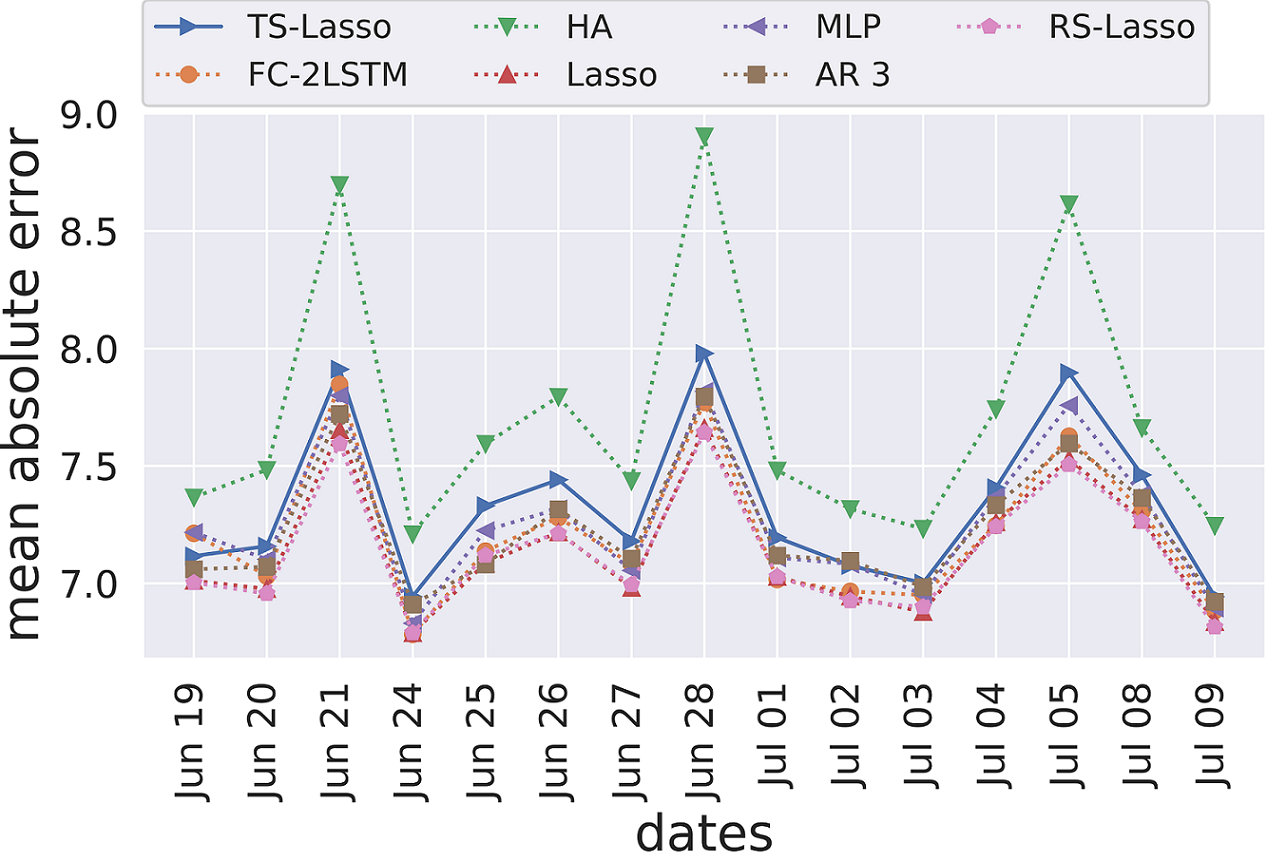
Figure 2: MSE and MAE computed (a) for each day and (b) for each specific hour.

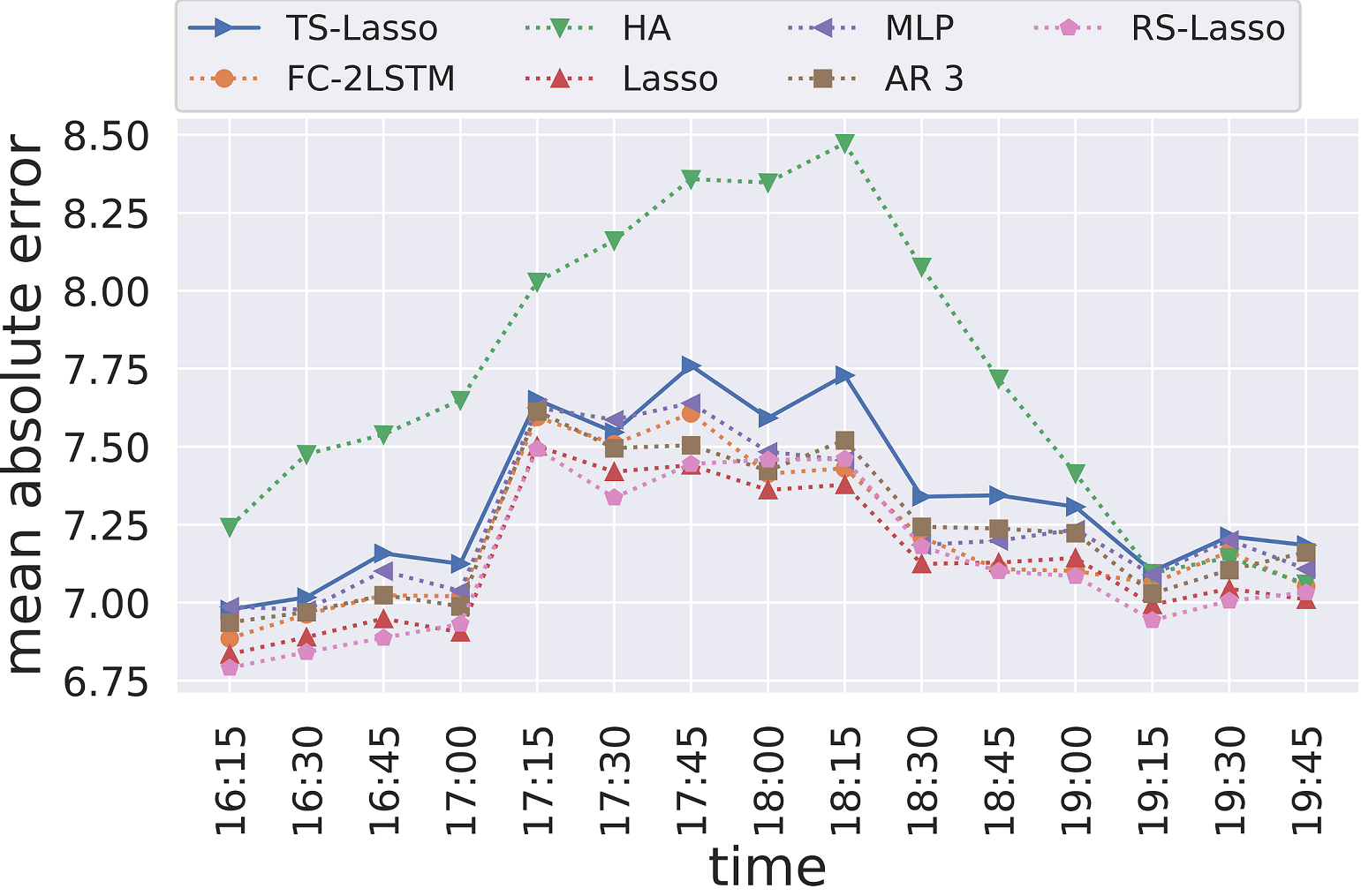
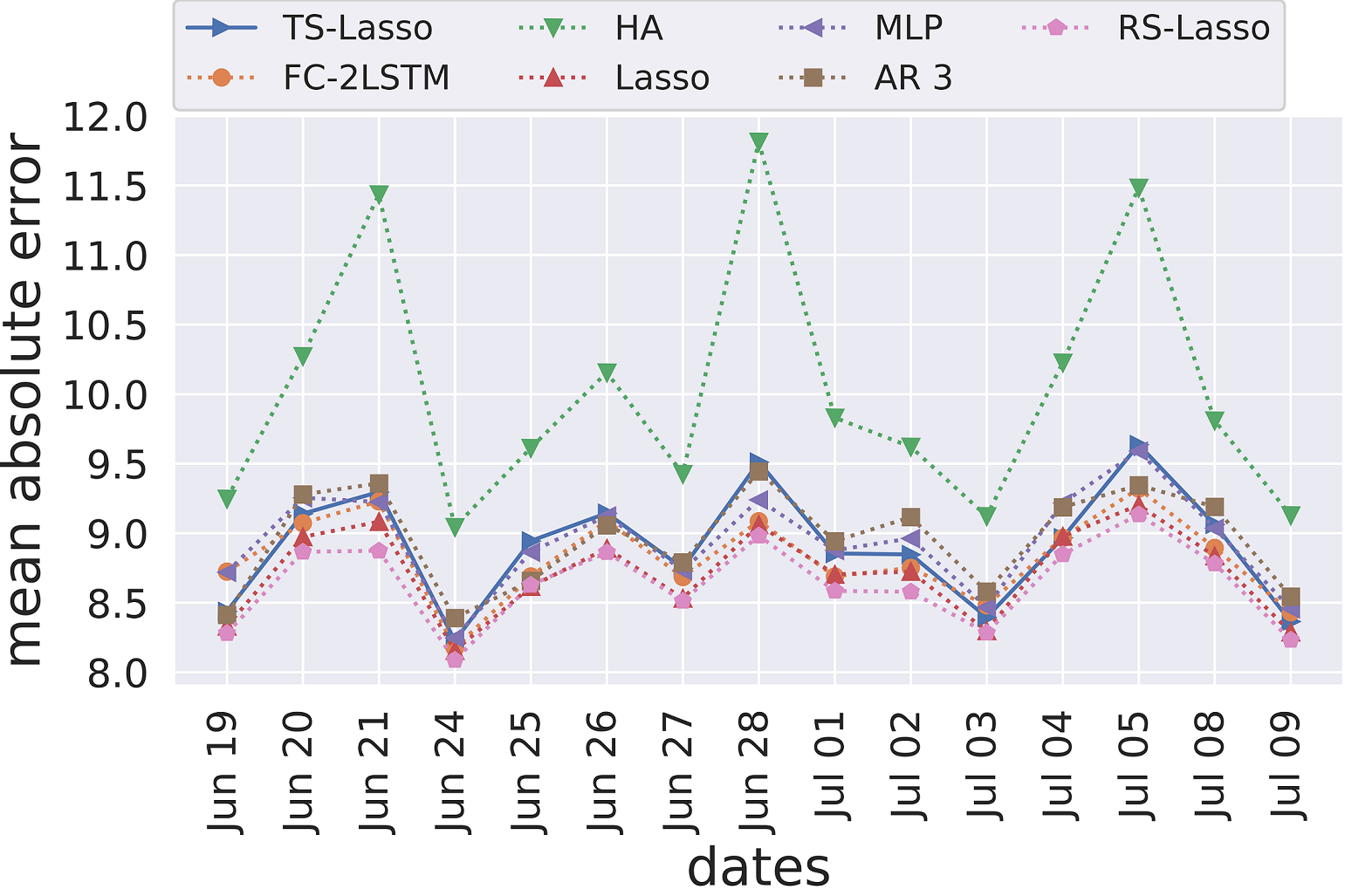
Table 1 shows the performance of all models over the entire network. The simple OLS model does not generalize well together with PO prediction; they yield the worst performances. The OLS is subjected to an over-fitting problem as the MAE is equal to 9.209.209.20 (resp. 5.695.695.69) on the test set (resp. train set). Other baseline performances are similar with AR, yielding a slightly better performance than the HA. Note that increasing the number of lags does not lead to better results. The neural networks offer close results to those of the AR with the LSTM performing slightly better than the MLP model. The different LASSO approaches also yielded variable results; the model with regime-switching (RS-LASSO with a time switch at 666:151515pm) performs better than all other models (7.137.137.13 MAE) and is just slightly better than the LASSO (0.010.01-0.01 MAE). Using a different LASSO predictor for each time (TS-LASSO) does not improve the error and yields a worse performance than the LASSO (+0.200.20+0.20 MAE). The same observation on Grp-LASSO suggests that entirely filtering some sections causes a certain loss.

In Figure 2, we present (a) the error computed for each specific day (large errors correspond to fridays) and (b) the error for each specific hour (averaged over the days). For readability, we only present a subset of the models. The figure shows the LASSO and the RS-LASSO results over days and time and confirms that they outperform all other models. The two approaches alternate performance over time, we notice that the RS-LASSO performs better at the first and the last 1.51.51.5 hours and is worse than the LASSO in the middle hours. As this cut-off is happening around the switch to the RS-LASSO (666:151515pm), it might be possible that the RS-LASSO parts (before and after switching) focus on modeling the regime of the corresponding periods and overlooks the middle period that is separated by the time switch.

Performance on highly variable sections

To further understand the results, we compare the models on highly variable sections. Variable sections are selected based on a clustering algorithm applied to descriptive statistics (Min, Max, Mean, standard deviation, Quartiles) and computed for each section at each time. The cluster represents about 30%percent3030\% of the sections.

Model AR 1 AR 3 AR 5 FC-2LSTM HA LASSO MLP OLS PO RS-LASSO TS-LASSO Grp-LASSO
MAE 9.27 9.26 9.27 9.11 10.18 9.01 9.17 11.50 11.81 8.94 9.20 9.17
MSE 172.59 171.94 171.98 163.45 207.18 161.29 165.39 238.91 274.92 159.66 168.01 165.28
Table 2: MSE and MAE restricted to highly variable sections and computed (a) for each day and (b) for each specific hour.
Refer to caption
(a)
Refer to caption
(b)
Figure 3: The prediction error for each method (a) over days, (b) over time.

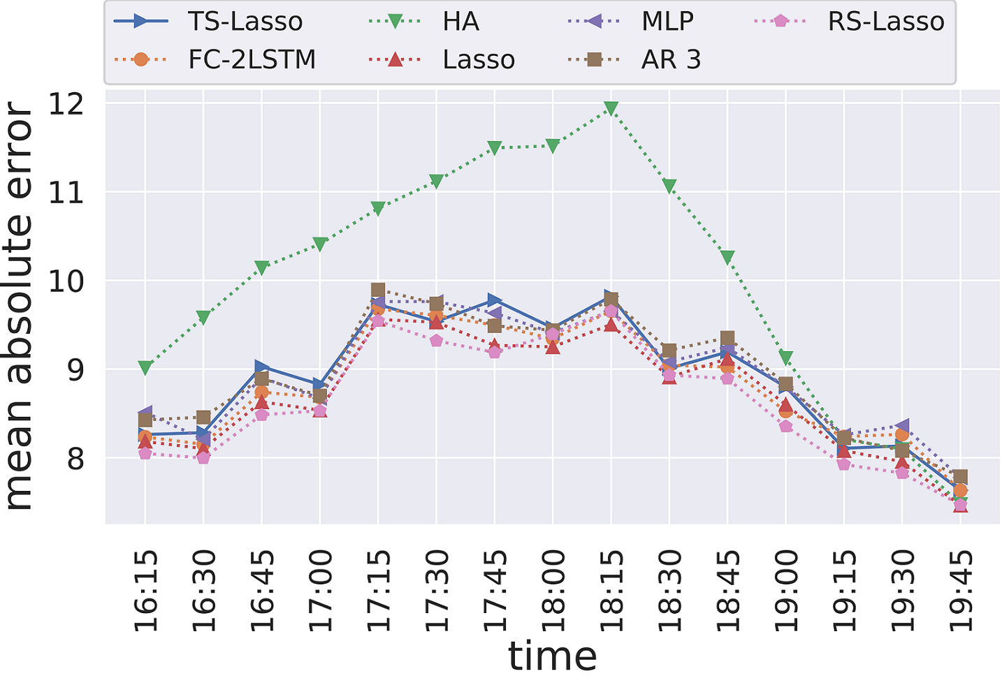
Table 2 and Figure 3 show the performance over highly variable sections only. All model performances deteriorate compared to the performances on the full road network. Similar observations as before can be made on these results with the exceptions that both neural networks, TS-LASSO and Grp-LASSO, perform better than the autoregressive models (0.20.2-0.2 MAE) . The performance gap between the models is wider. The RS-LASSO is clearly better than the LASSO (0.070.07-0.07 MAE) compared to the observed performance on the entire network. The alternation of performance over time is still observable between the LASSO and RS-LASSO models.

Comparison of different penalties

We now compare the performances between the LASSO, Ridge and Elastic Net penalties defined as:

  • LASSO (1subscript1\ell_{1}) penalty : wλw1maps-to𝑤𝜆subscriptnorm𝑤1w\mapsto\lambda||w||_{1}.

  • Ridge (2subscript2\ell_{2}) penalty : wλw22maps-to𝑤𝜆subscriptsuperscriptnorm𝑤22w\mapsto\lambda||w||^{2}_{2}.

  • Elastic Net penalty: wλ(αw1+(1α)w22)maps-to𝑤𝜆𝛼subscriptnorm𝑤11𝛼subscriptsuperscriptnorm𝑤22w\mapsto\lambda(\alpha||w||_{1}+(1-\alpha)||w||^{2}_{2}).

where λ𝜆\lambda is the regularization parameter and α[0.1,0.9]𝛼0.10.9\alpha\in[0.1,0.9] represents some ratio between the LASSO and Ridge penalties. For each method, λ𝜆\lambda and α𝛼\alpha are determined through the application of a 555-fold cross-validation. For Elastic Net, the best α𝛼\alpha was around 0.60.60.6 giving the 1subscript1\ell_{1}-penalty at a slightly higher weight.

Penalty OLS (No penalty) LASSO Ridge ElasticNet
MSE 162.83 105.89 110.78 108.48
MAE 9.22 7.00 7.15 7.09
Table 3: MSE and MAE computed over the whole network and the whole time period for the penalties LASSO, Ridge, Elastic Net.

Table 3 shows the obtained MAE and MSE for all the models. The LASSO penalty shows a slightly better performance than the other two penalties. This can be explained by the ability of the LASSO to effectively select features for the model which is increasingly important in a sparse, high dimensional setup. Therefore, choosing the 1subscript1\ell_{1}-penalty for this problem seems to be efficient and also gives a better interpretation of the model’s parameters.

5.3 Graphical visualization of the LASSO model

In this section, the aim is to show that the LASSO coefficients are interpretable and can be used to capture certain features of the architecture of the road network.

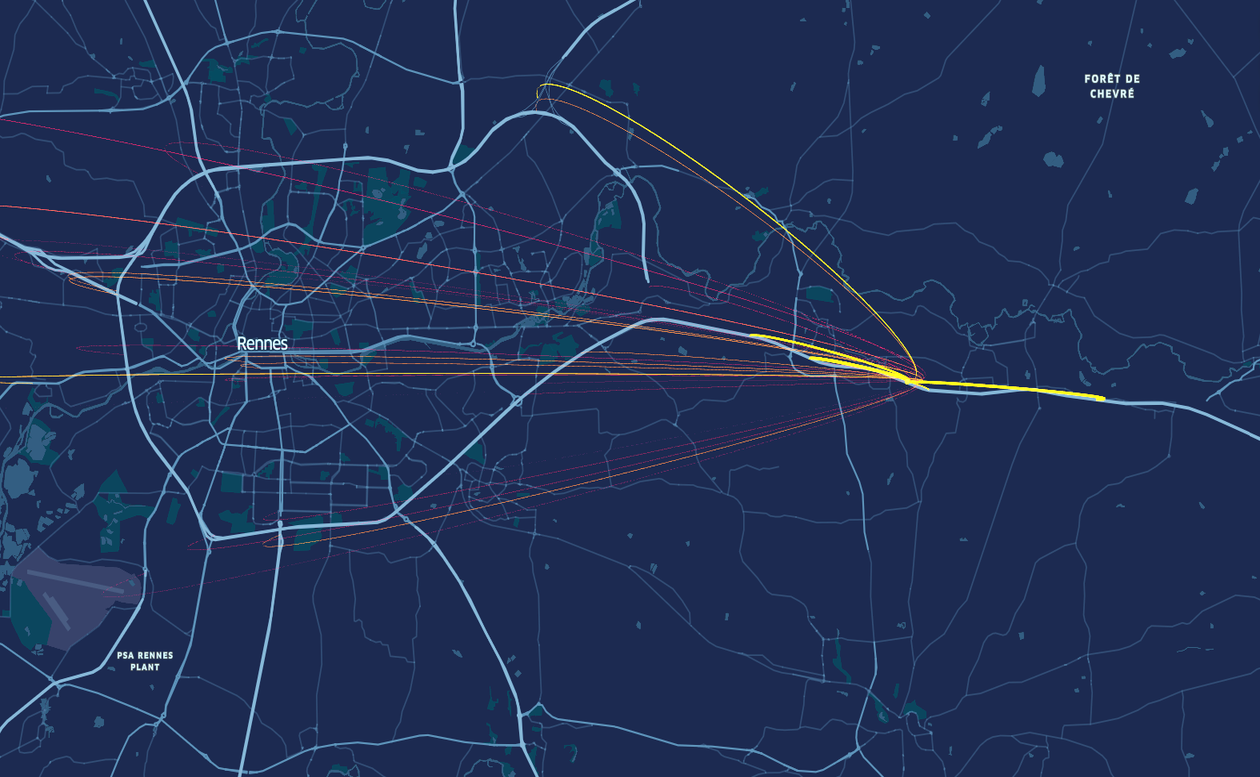
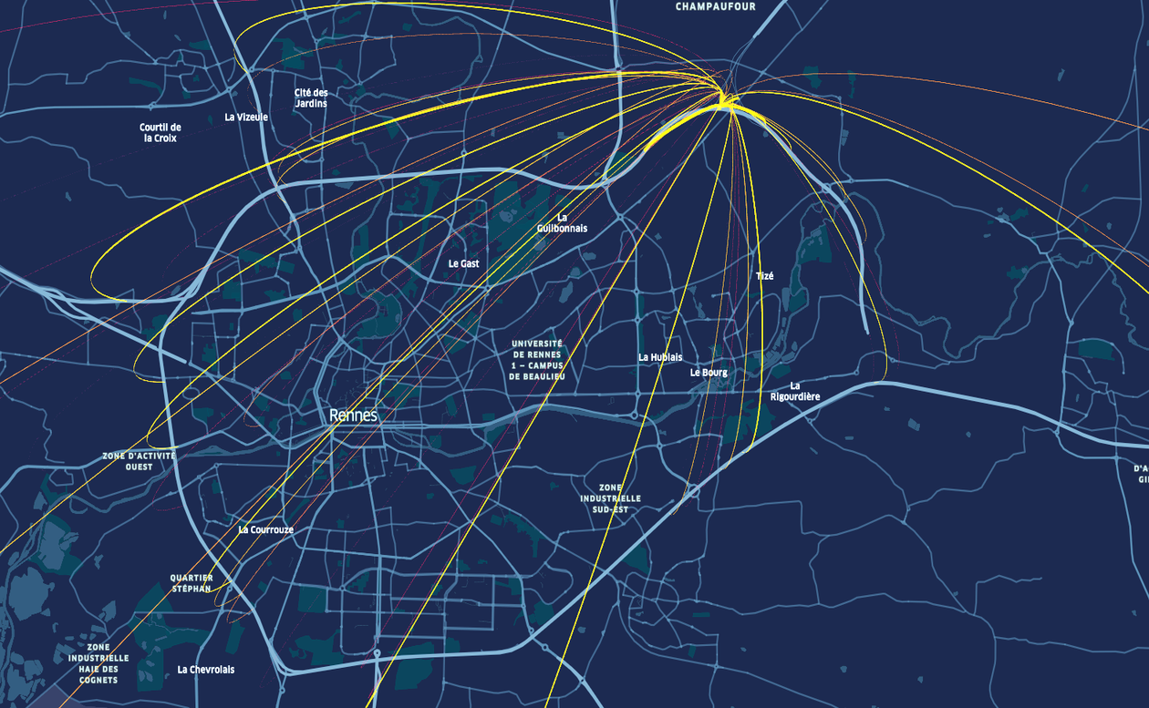
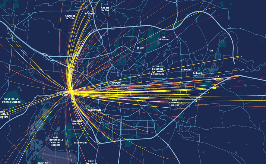
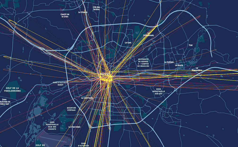
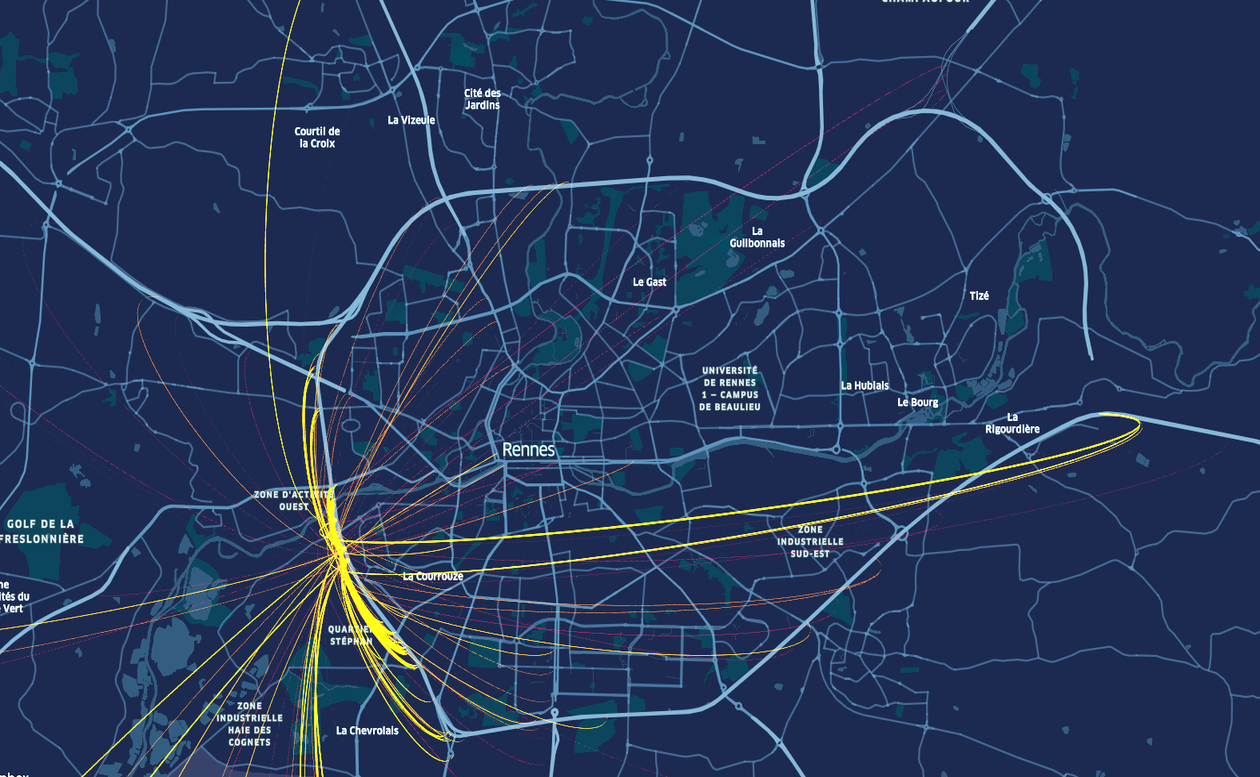
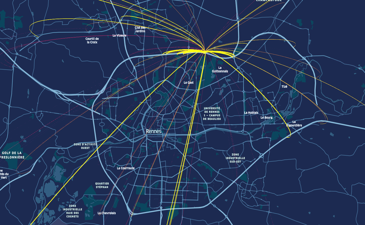
The LASSO coefficients are indicators of the traffic flow dependencies between the sections of the road network. For a section of interest, say k𝑘k, a way to visualize these connections is to draw, on top of the network map, arcs going from section k𝑘k to sections for which the corresponding regression coefficient is non-zero (that belongs to the active sets Sksubscriptsuperscript𝑆𝑘S^{\star}_{k}). In addition, the color intensity and the width of each arc can be scaled by the value of the corresponding coefficient in order to highlight the influence of one section on another.
Refer to caption
(a)
Refer to caption
(b)
Refer to caption
(c)
Refer to caption
(d)
Refer to caption
(e)
Refer to caption
(f)
Figure 4: For each graph, arcs are drawn from the section of interest to the active sections deduced from the estimated matrix coefficients A^(lasso)superscript^𝐴𝑙𝑎𝑠𝑠𝑜\hat{A}^{(lasso)}. Color intensity and width are scaled according to the value of the matrix coefficients. Different types of section are considered: (a) and (b) ring roads; (c) highway; (d,e) link roads; (f) city center.

The previous visualization is provided for several representative sections in Figure 4. In Figure 4, (a, b) represents sections from the Rennes ring roads, or beltways. These roads have an upper limit of 70km/h70𝑘𝑚70km/h and circles the whole city of Rennes. We see that these sections strongly connect to adjacent sections in the ring and also to the closest highways. This is expected as these sections are physically connected to each other as they form a ring road and have links to adjacent highways. We also observe this kind of behavior on the highways (Figure 4.c) where the sections of the highway have a higher dependence on adjacent sections of the highway. In Figure 4, (d, e), we show sections that are part of link roads, or bypasses. We see that these sections have a high number of connections to adjacent ring roads. These link roads usually connect the flow between relatively distant parts of the city so we also observe farther connections around the ring network. We observe similar aspects with sections from the city center as shown in Figure 4, (f).

Another meaningful visualization provided by the model consists of representing the influence of each section on the overall network using the values of the estimated coefficients. For section \ell, the criterion is given by C=1kp,A^k(lasso)>0Aksubscript𝐶subscriptformulae-sequence1𝑘𝑝superscriptsubscript^𝐴𝑘𝑙𝑎𝑠𝑠𝑜0subscript𝐴𝑘C_{\ell}=\sum_{1\leqslant k\leqslant p,\hat{A}_{k\ell}^{(lasso)}>0}A_{k\ell}. Taking into account negative coefficients implies an inverse relationship between sections, meaning that when a section is getting congested, another is getting less traffic. This may happen when there are incidents on the road but does not characterize the average influence between sections. Thus we only consider positive coefficients in building the criterion (consisting of 93%percent9393\% of the coefficients).

Refer to caption
Refer to caption
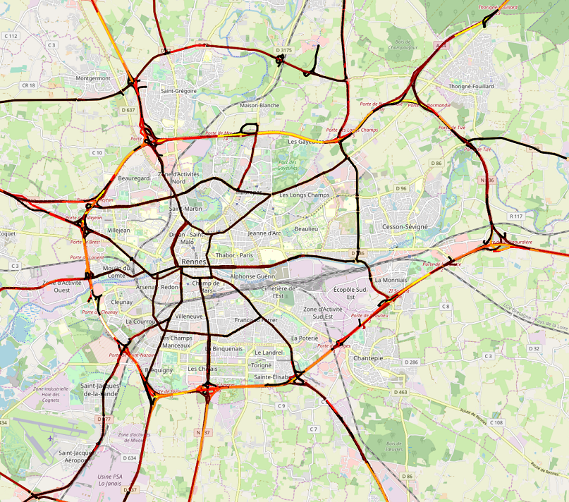
Figure 5: Heatmap plot of the sections based on the influence criterion Csubscript𝐶C_{\ell}.

Figure 5 is a heatmap of the road network where each section is color-coded according to the influence coefficient Csubscript𝐶C_{\ell}. We see that the network behavior is mainly influenced by ring road sections and highways. This is expected as traffic mainly flows on these roads as opposed to most sections in the city center, and those in the rural and suburban areas, that carries smaller quantities of traffic.

6 Simulation study

In this section, we present a data generation process which produces time-series that behave similarly to road traffic data. We then use the output to validate the regime switching approach by comparing it to other baseline algorithms.

6.1 Data generation process

Model parameters

The intercept sequence (bt)t=t,,Tsubscriptsubscript𝑏𝑡𝑡𝑡𝑇(b_{t})_{t=t,\ldots,T} is defined as follows. For each t{1,,T}𝑡1𝑇t\in\{1,\ldots,T\} and k{1,,p}𝑘1𝑝k\in\{1,\ldots,p\}, (bt)k=(2.52(t17.5)2)subscriptsubscript𝑏𝑡𝑘superscript2.52superscript𝑡17.52(b_{t})_{k}=-(2.5^{2}-(t-17.5)^{2}). The matrix A𝐴A is constructed as follows.

  • Generate an Erdös-Rényi graph (Erdős and Rényi, , 1959) with an average of 888 connections for each node in the network. This results in a sparse structure for the matrix A𝐴A.

  • Generate independently the nonzero entries of the matrix A𝐴A according to a uniform distribution on [1,1]11[-1,1].

  • Normalize the matrix so that each line has an 2subscript2\ell_{2}-norm equal to 111.

The last step above helps to obtain reasonable dynamics for the sequences of interest, for which the generation is described below.

Generation of the sequence

Let b𝑏b be an intercept matrix and let A𝐴A and Asuperscript𝐴A^{\prime} be two matrices constructed as before. For each day {1n}1𝑛\{1\dots n\}, the initial speed vector W0(i)superscriptsubscript𝑊0𝑖W_{0}^{(i)} of size p𝑝p has independent entries distributed as a mixture between 333 Gaussian distributions (to get roughly 333 different classes of speed) given by

0.25𝒩(S1,0.1S1/2)+0.5𝒩(S2,0.1S2/2)+0.25𝒩(S3,0.1S3/2),0.25𝒩subscript𝑆10.1subscript𝑆120.5𝒩subscript𝑆20.1subscript𝑆220.25𝒩subscript𝑆30.1subscript𝑆320.25\mathcal{N}(S_{1},0.1S_{1}/2)+0.5\mathcal{N}(S_{2},0.1S_{2}/2)+0.25\mathcal{N}(S_{3},0.1S_{3}/2),

with S1=45subscript𝑆145S_{1}=45, S2=72subscript𝑆272S_{2}=72 and S3=117subscript𝑆3117S_{3}=117. Generate (ϵt(i))t=1,Tpsubscriptsuperscriptsubscriptitalic-ϵ𝑡𝑖𝑡1𝑇superscript𝑝(\epsilon_{t}^{(i)})_{t=1,\ldots T}\subset\mathbb{R}^{p} as an independent and identically distributed sequence with distribution 𝒩(0,Ip)𝒩0subscript𝐼𝑝\mathcal{N}(0,I_{p}). The data is then obtained based on

Wt+1(i)=bt+A(Wt(i)𝔼[Wt(i)])+ϵt(i),t=1,,11,formulae-sequencesuperscriptsubscript𝑊𝑡1𝑖subscript𝑏𝑡𝐴superscriptsubscript𝑊𝑡𝑖𝔼delimited-[]superscriptsubscript𝑊𝑡𝑖superscriptsubscriptitalic-ϵ𝑡𝑖𝑡111\displaystyle W_{t+1}^{(i)}=b_{t}+A(W_{t}^{(i)}-\mathbb{E}[W_{t}^{(i)}])+\epsilon_{t}^{(i)},\qquad t=1,\ldots,11,
Wt+1(i)=bt+A(Wt(i)𝔼[Wt(i)])+ϵt(i),t=12,,18.formulae-sequencesuperscriptsubscript𝑊𝑡1𝑖subscript𝑏𝑡superscript𝐴superscriptsubscript𝑊𝑡𝑖𝔼delimited-[]superscriptsubscript𝑊𝑡𝑖superscriptsubscriptitalic-ϵ𝑡𝑖𝑡1218\displaystyle W_{t+1}^{(i)}=b_{t}+A^{\prime}(W_{t}^{(i)}-\mathbb{E}[W_{t}^{(i)}])+\epsilon_{t}^{(i)},\qquad t=12,\ldots,18.

6.2 Results

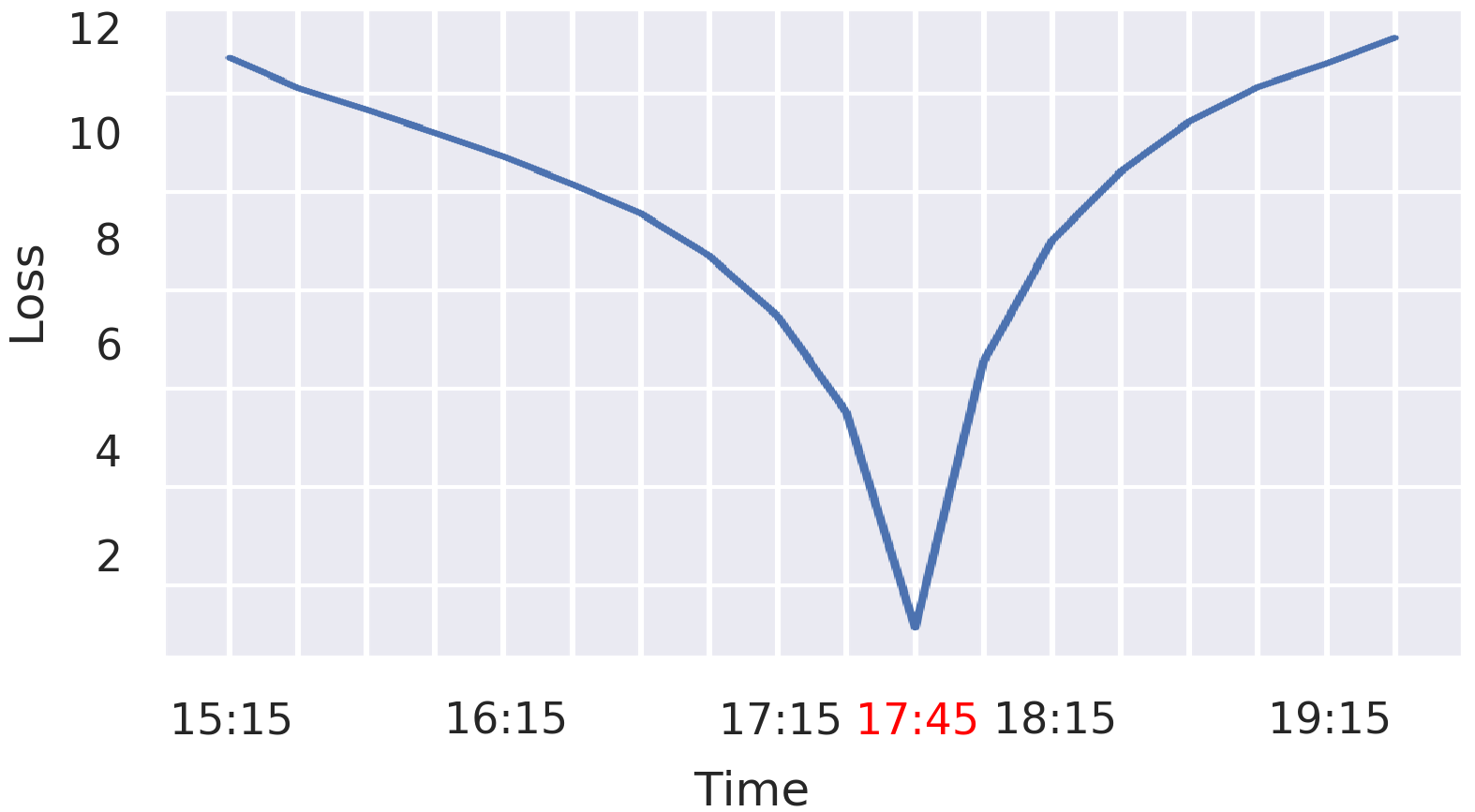
The RS-LASSO approach introduced in Section 4 results from a search of the best instant t𝑡t from which a different (linear) model shall be used. This search is conducted by comparing the estimated risks R^tsubscript^𝑅𝑡\hat{R}_{t}, t=1,,T𝑡1𝑇t=1,\ldots,T, where t𝑡t is the instant from which a second model is estimated.
Refer to caption
Figure 6: Evolution of the estimated risks R^tsubscript^𝑅𝑡\hat{R}_{t}.

Figure 6 represents the evolution of the estimated risks for a single representative dataset. The best change point can be easily identified as the procedure gives t^=11^𝑡11\hat{t}=11.

Model OLS MLP FC-2LSTM AR 1 AR 3 AR 5 HA PO LASSO Grp-LASSO RS-LASSO TS-LASSO
MSE 18.94 16.13 17.43 52.55 45.11 44.9 60.32 110.68 13.97 14.81 1.13 5.30
MAE 3.24 2.96 3.13 5.65 5.21 5.2 6.04 7.95 2.75 2.85 0.85 1.75
Table 4: MSE and MAE computed over the whole network and the whole time period.

In Table 4, we compare the RS-LASSO to the other methods based on M=20𝑀20M=20 independent datasets (the MSE and MAE have been averaged over the datasets). The RS-LASSO model obtains the best performance and clearly outperforms the other methods. The fact that RS-LASSO succeeds in identifying the exact switching time allows for the build-up of considerably good predictors for both time-windows before and after the switch. Nonlinear models such as MLP and LSTM obtained slightly lower performances than the LASSO and slightly better than OLS. The baseline methods HA, PO, and AR gave the worst performance on the simulated data (as well as on the real data). In short, we can distinguish between four classes of methods reflecting their level of performance. Baseline methods give the worst results. The one-model methods (LASSO, OLS, Grp-LASSO, MLP, LSTM) give reasonable results. The multiple-model TS-LASSO works better than one-model methods and finally, the regime-switching RS-LASSO performs the best (by fitting only two models to the data).

FD(RS-LASSO) FD( LASSO) SR(RS-LASSO) SR( LASSO)
Left model 1.592872 19.755836 96.49% 79.11%
Right model 1.301384 18.232622 96.37% 79.22%
Table 5: Frobenius distance and support recovery rate for LASSO and RS-LASSO.

In order to further investigate the RS-LASSO model, we compare the estimated matrices A^^𝐴\hat{A} and A^superscript^𝐴\hat{A}^{\prime} to the ones used in the data generation process. Table 5 shows the Frobenius distance (FD) A^AF+A^AFsubscriptnorm^𝐴𝐴𝐹subscriptnormsuperscript^𝐴superscript𝐴𝐹\|\hat{A}-A\|_{F}+\|\hat{A}^{\prime}-A^{\prime}\|_{F} along with the support recovery rates (SR)𝑆𝑅(SR) defined as the percentage of accordance in the non-zero coefficients (active set) between the estimated matrix and the truth. In contrast with the LASSO, we observe a very small Frobenius error for RS-LASSO. In the meantime, the support recovery of RS-LASSO is more than 96%percent9696\% compared to around 79%percent7979\% for the LASSO. This confirms the favorable performance of RS-LASSO.

7 Conclusion

We proposed in this paper a methodology to model high-dimensional time-series for which regeneration occurs at the end of each day. In a high-dimensional setting, we established bounds on the prediction error associated to linear predictors. More precisely, we showed that the regularized least-squares approach provides a decrease of the prediction error bound compared to ordinary least-squares. In addition, a regime switching detection procedure has been proposed and its consistency has been established. Through simulations and using floating car data observed in an urban area, the proposed approach has been compared to several other methods. Further research might be conducted on the extension of the proposed approach to general Markov chains. In this case, the regeneration times are unobserved and occur randomly involving a completely different probabilistic setting than the one borrowed in this paper. Whereas regeneration properties are known to be powerful theoretical tools to study estimates based on Markov Chains (see e.g., (Bertail and Portier, , 2019) for a recent account), their use in a prediction framework seems not to have been investigated. Another possible extension concerns the identification of multiple change points. On the theoretical side, the consistency of the proposed cross-validation procedure has been established in Section 4 only when a unique change point occurs.

Acknowledgment

The authors are grateful to Maxime Bourliatoux for helpful discussions on an earlier version of this work and Bethany Cagnol for assistance in proof reading the article. This work was financially supported by the FUI 22 GEOLYTICS project. The authors would like to thank IT4PME and Coyote for providing data and for their support.

References

  • Baek et al., (2017) Baek, C., Davis, R. A., and Pipiras, V. (2017). Sparse seasonal and periodic vector autoregressive modeling. Computational Statistics & Data Analysis, 106:103–126.
  • Basu et al., (2015) Basu, S., Michailidis, G., et al. (2015). Regularized estimation in sparse high-dimensional time series models. The Annals of Statistics, 43(4):1535–1567.
  • Bertail and Portier, (2019) Bertail, P. and Portier, F. (2019). Rademacher complexity for markov chains: Applications to kernel smoothing and metropolis–hastings. Bernoulli, 25(4B):3912–3938.
  • Bickel et al., (2009) Bickel, P. J., Ritov, Y., Tsybakov, A. B., et al. (2009). Simultaneous analysis of lasso and dantzig selector. The Annals of Statistics, 37(4):1705–1732.
  • Brockwell et al., (1991) Brockwell, P. J., Davis, R. A., and Fienberg, S. E. (1991). Time Series: Theory and Methods: Theory and Methods. Springer Science & Business Media.
  • Broock et al., (1996) Broock, W. A., Scheinkman, J. A., Dechert, W. D., and LeBaron, B. (1996). A test for independence based on the correlation dimension. Econometric reviews, 15(3):197–235.
  • Bühlmann and Van De Geer, (2011) Bühlmann, P. and Van De Geer, S. (2011). Statistics for high-dimensional data: methods, theory and applications. Springer Science & Business Media.
  • Bull, (2003) Bull, A. (2003). 1, 2, 6. United Nations, Economic Commission for Latin America and the Caribbean.
  • Bunea et al., (2007) Bunea, F., Tsybakov, A., Wegkamp, M., et al. (2007). Sparsity oracle inequalities for the lasso. Electronic Journal of Statistics, 1:169–194.
  • Caruana et al., (2001) Caruana, R., Lawrence, S., and Giles, C. L. (2001). Overfitting in neural nets: Backpropagation, conjugate gradient, and early stopping. In Advances in neural information processing systems, pages 402–408.
  • Dai et al., (2017) Dai, X., Fu, R., Lin, Y., Li, L., and Wang, F.-Y. (2017). Deeptrend: A deep hierarchical neural network for traffic flow prediction. arXiv preprint arXiv:1707.03213.
  • Davis et al., (2016) Davis, R. A., Zang, P., and Zheng, T. (2016). Sparse vector autoregressive modeling. Journal of Computational and Graphical Statistics, 25(4):1077–1096.
  • Epelbaum et al., (2017) Epelbaum, T., Gamboa, F., Loubes, J.-M., and Martin, J. (2017). Deep learning applied to road traffic speed forecasting. arXiv preprint arXiv:1710.08266.
  • Erdős and Rényi, (1959) Erdős, P. and Rényi, A. (1959). On random graphs i. Publ. math. debrecen, 6(290-297):18.
  • Giraud, (2014) Giraud, C. (2014). Introduction to high-dimensional statistics, volume 138. CRC Press.
  • Greenfeld, (2002) Greenfeld, J. S. (2002). Matching gps observations to locations on a digital map. In 81th annual meeting of the transportation research board, volume 1, pages 164–173. Washington, DC.
  • Hamilton, (1994) Hamilton, J. D. (1994). Time series analysis, volume 2. Princeton university press Princeton, NJ.
  • Harrison and Donnelly, (2011) Harrison, C. and Donnelly, I. A. (2011). A theory of smart cities. In Proceedings of the 55th Annual Meeting of the ISSS-2011, Hull, UK, volume 55.
  • Hastie et al., (2015) Hastie, T., Tibshirani, R., and Wainwright, M. (2015). Statistical learning with sparsity: the lasso and generalizations. Chapman and Hall/CRC.
  • Haufe et al., (2010) Haufe, S., Müller, K.-R., Nolte, G., and Krämer, N. (2010). Sparse causal discovery in multivariate time series. In Causality: Objectives and Assessment, pages 97–106.
  • Kock and Callot, (2015) Kock, A. B. and Callot, L. (2015). Oracle inequalities for high dimensional vector autoregressions. Journal of Econometrics, 186(2):325–344.
  • Li et al., (2017) Li, Y., Yu, R., Shahabi, C., and Liu, Y. (2017). Diffusion convolutional recurrent neural network: Data-driven traffic forecasting. arXiv preprint arXiv:1707.01926.
  • Lv et al., (2014) Lv, Y., Duan, Y., Kang, W., Li, Z., and Wang, F.-Y. (2014). Traffic flow prediction with big data: a deep learning approach. IEEE Transactions on Intelligent Transportation Systems, 16(2):865–873.
  • Lv et al., (2018) Lv, Z., Xu, J., Zheng, K., Yin, H., Zhao, P., and Zhou, X. (2018). Lc-rnn: A deep learning model for traffic speed prediction. In IJCAI, pages 3470–3476.
  • Meyn and Tweedie, (2012) Meyn, S. P. and Tweedie, R. L. (2012). Markov chains and stochastic stability. Springer Science & Business Media.
  • Michailidis and d’Alché Buc, (2013) Michailidis, G. and d’Alché Buc, F. (2013). Autoregressive models for gene regulatory network inference: Sparsity, stability and causality issues. Mathematical biosciences, 246(2):326–334.
  • Pellicer et al., (2013) Pellicer, S., Santa, G., Bleda, A. L., Maestre, R., Jara, A. J., and Skarmeta, A. G. (2013). A global perspective of smart cities: A survey. In 2013 Seventh International Conference on Innovative Mobile and Internet Services in Ubiquitous Computing, pages 439–444. IEEE.
  • Song and Bickel, (2011) Song, S. and Bickel, P. J. (2011). Large vector auto regressions. arXiv preprint arXiv:1106.3915.
  • Tibshirani, (1996) Tibshirani, R. (1996). Regression shrinkage and selection via the lasso. Journal of the Royal Statistical Society: Series B (Methodological), 58(1):267–288.
  • Valdés-Sosa et al., (2005) Valdés-Sosa, P. A., Sánchez-Bornot, J. M., Lage-Castellanos, A., Vega-Hernández, M., Bosch-Bayard, J., Melie-García, L., and Canales-Rodríguez, E. (2005). Estimating brain functional connectivity with sparse multivariate autoregression. Philosophical Transactions of the Royal Society B: Biological Sciences, 360(1457):969–981.
  • Van De Geer and Bühlmann, (2009) Van De Geer, S. A. and Bühlmann, P. (2009). On the conditions used to prove oracle results for the lasso. Electronic Journal of Statistics, 3:1360–1392.
  • Wang et al., (2007) Wang, H., Li, G., and Tsai, C.-L. (2007). Regression coefficient and autoregressive order shrinkage and selection via the lasso. Journal of the Royal Statistical Society: Series B (Statistical Methodology), 69(1):63–78.
  • Washburn et al., (2009) Washburn, D., Sindhu, U., Balaouras, S., Dines, R. A., Hayes, N., and Nelson, L. E. (2009). Helping cios understand “smart city” initiatives. Growth, 17(2):1–17.

Appendix A Proofs of the stated results

Before starting the proofs, we specify some useful notations. For any matrix Mp×T𝑀superscript𝑝𝑇M\in\mathbb{R}^{p\times T}, the 1subscript1\ell_{1}-norm is denoted by M1=k=1pt=1T|Mk,t|subscriptnorm𝑀1superscriptsubscript𝑘1𝑝superscriptsubscript𝑡1𝑇subscript𝑀𝑘𝑡\|M\|_{1}=\sum_{k=1}^{p}\sum_{t=1}^{T}|M_{k,t}| and the subscript\ell_{\infty}-norm is given by M=maxk=1,,p,t=1,,T|Mk,t|subscriptnorm𝑀subscriptformulae-sequence𝑘1𝑝𝑡1𝑇subscript𝑀𝑘𝑡\|M\|_{\infty}=\max_{k=1,\ldots,p,\,t=1,\ldots,T}|M_{k,t}|. The t𝑡t-th column (resp. k𝑘k-th line) of M𝑀M is denoted by M{,t}psubscript𝑀𝑡superscript𝑝M_{\{\cdot,t\}}\in\mathbb{R}^{p} (resp M{k,}Tsubscript𝑀𝑘superscript𝑇M_{\{k,\cdot\}}\in\mathbb{R}^{T}). Both are column vectors.

A.1 Proof of Proposition 1

Denote by L2(P)subscript𝐿2𝑃L_{2}(P) the Hilbert space composed of the random elements W𝑊W defined on (Ω,,P)Ω𝑃(\Omega,\mathcal{F},P) such that EWF<+𝐸subscriptnorm𝑊𝐹E\|W\|_{F}<+\infty. The underlying scalar product between X𝑋X and Y𝑌Y is tr(E[XTY])tr𝐸delimited-[]superscript𝑋𝑇𝑌\operatorname{tr}(E[X^{T}Y]). Hence infLE[YL(X)F2]subscriptinfimum𝐿𝐸delimited-[]superscriptsubscriptnorm𝑌𝐿𝑋𝐹2\inf_{L\in\mathcal{L}}E[\|Y-L(X)\|_{F}^{2}] is a distance between the element Y𝑌Y of L2(P)subscript𝐿2𝑃L_{2}(P) and the linear subspace of L2(P)subscript𝐿2𝑃L_{2}(P) made of L(X)𝐿𝑋L(X), L𝐿L\in\mathcal{L}. The Hilbert projection theorem ensures that the infimum is uniquely achieved and that L(X)superscript𝐿𝑋L^{\star}(X) is the argument of the minimum if and only if tr(E[(YL(X))TL(X)])=0tr𝐸delimited-[]superscript𝑌superscript𝐿𝑋𝑇𝐿𝑋0\operatorname{tr}(E[(Y-L^{\star}(X))^{T}L(X)])=0 for all L𝐿L\in\mathcal{L}. Taking A=0𝐴0A=0, in L(X)=b+AX𝐿𝑋𝑏𝐴𝑋L(X)=b+AX, gives the first set of normal equations. We conclude by taking b=0𝑏0b=0 and noting that tr(E[(YL(X))TL(X)])=tr(E[X(YL(X))T]A)=0tr𝐸delimited-[]superscript𝑌superscript𝐿𝑋𝑇𝐿𝑋tr𝐸delimited-[]𝑋superscript𝑌superscript𝐿𝑋𝑇𝐴0\operatorname{tr}(E[(Y-L^{\star}(X))^{T}L(X)])=\operatorname{tr}(E[X(Y-L^{\star}(X))^{T}]A)=0 for all Ap×p𝐴superscript𝑝𝑝A\in\mathbb{R}^{p\times p} is equivalent to E[(YL(X))XT]=0𝐸delimited-[]𝑌superscript𝐿𝑋superscript𝑋𝑇0E[(Y-L^{\star}(X))X^{T}]=0. This is the second set of normal equations. ∎

A.2 Proof of Proposition 2

The statement follows from developing pR(L)=E[(YL(X))+(L(X)L(X))2]𝑝𝑅𝐿𝐸delimited-[]superscriptnorm𝑌superscript𝐿𝑋superscript𝐿𝑋𝐿𝑋2pR(L)=E[\|(Y-L^{\star}(X))+(L^{\star}(X)-L(X))\|^{2}] and then using that tr(E[(YL(X))(L(X)L(X))T])=0tr𝐸delimited-[]𝑌superscript𝐿𝑋superscript𝐿𝑋superscript𝐿𝑋𝑇0\operatorname{tr}(E[(Y-L^{\star}(X))(L(X)-L^{\star}(X))^{T}])=0 which is a consequence of the normal equations given in Proposition 1. ∎

A.2.1 Proof of Proposition 3

Let Xc=XE[X]subscript𝑋𝑐𝑋𝐸delimited-[]𝑋X_{c}=X-E[X]. Recall that L^(X)=b^+A^X^𝐿𝑋^𝑏^𝐴𝑋\hat{L}(X)=\hat{b}+\hat{A}X and L(X)=E[Y]+AXcsuperscript𝐿𝑋𝐸delimited-[]𝑌superscript𝐴subscript𝑋𝑐L^{\star}(X)=E[Y]+A^{\star}X_{c}. In virtue of Proposition 2, we have

p(L^)𝑝^𝐿\displaystyle p\mathcal{E}(\hat{L}) =EX[(AA^)Xc+E(Y)A^E(X)b^F2],absentsubscript𝐸𝑋delimited-[]superscriptsubscriptnormsuperscript𝐴^𝐴subscript𝑋𝑐𝐸𝑌^𝐴𝐸𝑋^𝑏𝐹2\displaystyle=E_{X}[\|(A^{\star}-\hat{A})X_{c}+E(Y)-\hat{A}E(X)-\hat{b}\|_{F}^{2}],

where EXsubscript𝐸𝑋E_{X} stands for the expectation with respect to X𝑋X only. Because, Xcsubscript𝑋𝑐X_{c} has mean 00, we get

p(L^)𝑝^𝐿\displaystyle p\mathcal{E}(\hat{L}) =EX[(AA^)XcF2]+E(Y)A^E(X)b^F2.absentsubscript𝐸𝑋delimited-[]superscriptsubscriptnormsuperscript𝐴^𝐴subscript𝑋𝑐𝐹2superscriptsubscriptnorm𝐸𝑌^𝐴𝐸𝑋^𝑏𝐹2\displaystyle=E_{X}[\|(A^{\star}-\hat{A})X_{c}\|_{F}^{2}]+\|E(Y)-\hat{A}E(X)-\hat{b}\|_{F}^{2}.

Finally, since EX[(AA^)XcF2]=(AA^)Σ1/2F2subscript𝐸𝑋delimited-[]superscriptsubscriptnormsuperscript𝐴^𝐴subscript𝑋𝑐𝐹2superscriptsubscriptnormsuperscript𝐴^𝐴superscriptΣ12𝐹2E_{X}[\|(A^{\star}-\hat{A})X_{c}\|_{F}^{2}]=\|(A^{\star}-\hat{A})\Sigma^{1/2}\|_{F}^{2}, and using the triangle inequality, we find

p(L^)𝑝^𝐿\displaystyle p\mathcal{E}(\hat{L}) (AA^)Σ1/2F2+2E(Y)Y¯nF2+2A^(E(X)X¯n)F2.absentsuperscriptsubscriptnormsuperscript𝐴^𝐴superscriptΣ12𝐹22superscriptsubscriptnorm𝐸𝑌superscript¯𝑌𝑛𝐹22superscriptsubscriptnorm^𝐴𝐸𝑋superscript¯𝑋𝑛𝐹2\displaystyle\leqslant\|(A^{\star}-\hat{A})\Sigma^{1/2}\|_{F}^{2}+2\|E(Y)-\overline{Y}^{n}\|_{F}^{2}+2\|\hat{A}(E(X)-\overline{X}^{n})\|_{F}^{2}.

A.2.2 Proof of Proposition 4

The inequality of Proposition 3 applied to the OLS estimate gives

p(L^(ols))(AA^(ols))Σ1/2F2+2Y¯nE(Y)F2+2A^(ols)Σ1/2Z¯nF2.𝑝superscript^𝐿𝑜𝑙𝑠superscriptsubscriptnormsuperscript𝐴superscript^𝐴𝑜𝑙𝑠superscriptΣ12𝐹22superscriptsubscriptnormsuperscript¯𝑌𝑛𝐸𝑌𝐹22superscriptsubscriptnormsuperscript^𝐴𝑜𝑙𝑠superscriptΣ12superscript¯𝑍𝑛𝐹2\displaystyle p\mathcal{E}(\hat{L}^{(ols)})\leqslant\|(A^{\star}-\hat{A}^{(ols)})\Sigma^{1/2}\|_{F}^{2}+2\|\overline{Y}^{n}-E(Y)\|_{F}^{2}+2\|\hat{A}^{(ols)}\Sigma^{1/2}\overline{Z}^{n}\|_{F}^{2}.

Using that A^(ols)Σ1/2Z¯nF(A^(ols)A)Σ1/2FZ¯nF+AΣ1/2Z¯nFsubscriptnormsuperscript^𝐴𝑜𝑙𝑠superscriptΣ12superscript¯𝑍𝑛𝐹subscriptnormsuperscript^𝐴𝑜𝑙𝑠superscript𝐴superscriptΣ12𝐹subscriptnormsuperscript¯𝑍𝑛𝐹subscriptnormsuperscript𝐴superscriptΣ12superscript¯𝑍𝑛𝐹\|\hat{A}^{(ols)}\Sigma^{1/2}\overline{Z}^{n}\|_{F}\leqslant\|(\hat{A}^{(ols)}-A^{\star})\Sigma^{1/2}\|_{F}\|\overline{Z}^{n}\|_{F}+\|A^{\star}\Sigma^{1/2}\overline{Z}^{n}\|_{F}, we get

p(L^(ols))(AA^(ols))Σ1/2F2(1+4Z¯nF2)+2Y¯nE(Y)F2𝑝superscript^𝐿𝑜𝑙𝑠superscriptsubscriptnormsuperscript𝐴superscript^𝐴𝑜𝑙𝑠superscriptΣ12𝐹214superscriptsubscriptnormsuperscript¯𝑍𝑛𝐹22superscriptsubscriptnormsuperscript¯𝑌𝑛𝐸𝑌𝐹2\displaystyle p\mathcal{E}(\hat{L}^{(ols)})\leqslant\|(A^{\star}-\hat{A}^{(ols)})\Sigma^{1/2}\|_{F}^{2}(1+4\|\overline{Z}^{n}\|_{F}^{2})+2\|\overline{Y}^{n}-E(Y)\|_{F}^{2}
+4AΣ1/2Z¯nF2.4superscriptsubscriptnormsuperscript𝐴superscriptΣ12superscript¯𝑍𝑛𝐹2\displaystyle+4\|A^{\star}\Sigma^{1/2}\overline{Z}^{n}\|_{F}^{2}.

Let ΓΓ\Gamma denote the greatest eigenvalue of ΣΣ\Sigma. By Assumption 3, we have lim supnΓ<subscriptlimit-supremum𝑛Γ\limsup_{n\to\infty}\Gamma<\infty. Applying Lemma 9, we deduce that

p(L^(ols))𝑝superscript^𝐿𝑜𝑙𝑠\displaystyle p\mathcal{E}(\hat{L}^{(ols)}) =(AA^(ols))Σ1/2F2(1+OP(pn))+OP(p+AΣ1/2F2n)absentsuperscriptsubscriptnormsuperscript𝐴superscript^𝐴𝑜𝑙𝑠superscriptΣ12𝐹21subscript𝑂𝑃𝑝𝑛subscript𝑂𝑃𝑝superscriptsubscriptnormsuperscript𝐴superscriptΣ12𝐹2𝑛\displaystyle=\|(A^{\star}-\hat{A}^{(ols)})\Sigma^{1/2}\|_{F}^{2}\left(1+O_{P}\left(\frac{p}{n}\right)\right)+O_{P}\left(\frac{p+\|A^{\star}\Sigma^{1/2}\|_{F}^{2}}{n}\right)
=(AA^(ols))Σ1/2F2OP(1)+OP(p+AΣ1/2F2n)absentsuperscriptsubscriptnormsuperscript𝐴superscript^𝐴𝑜𝑙𝑠superscriptΣ12𝐹2subscript𝑂𝑃1subscript𝑂𝑃𝑝superscriptsubscriptnormsuperscript𝐴superscriptΣ12𝐹2𝑛\displaystyle=\|(A^{\star}-\hat{A}^{(ols)})\Sigma^{1/2}\|_{F}^{2}O_{P}(1)+O_{P}\left(\frac{p+\|A^{\star}\Sigma^{1/2}\|_{F}^{2}}{n}\right)
=(AA^(ols))Σ1/2F2OP(1)+OP(p+ΓAF2n),absentsuperscriptsubscriptnormsuperscript𝐴superscript^𝐴𝑜𝑙𝑠superscriptΣ12𝐹2subscript𝑂𝑃1subscript𝑂𝑃𝑝Γsuperscriptsubscriptnormsuperscript𝐴𝐹2𝑛\displaystyle=\|(A^{\star}-\hat{A}^{(ols)})\Sigma^{1/2}\|_{F}^{2}O_{P}(1)+O_{P}\left(\frac{p+\Gamma\|A^{\star}\|_{F}^{2}}{n}\right), (5)

where we just used that p/n0𝑝𝑛0p/n\to 0 and AΣ1/2F2=k=1pA{k,}TΣ1/222ΓAF2superscriptsubscriptnormsuperscript𝐴superscriptΣ12𝐹2superscriptsubscript𝑘1𝑝superscriptsubscriptnormsubscriptsuperscript𝐴absent𝑇𝑘superscriptΣ1222Γsuperscriptsubscriptnormsuperscript𝐴𝐹2\|A^{\star}\Sigma^{1/2}\|_{F}^{2}=\sum_{k=1}^{p}\|A^{\star T}_{\{k,\cdot\}}\Sigma^{1/2}\|_{2}^{2}\leqslant\Gamma\|A^{\star}\|_{F}^{2}. Hence the proof of Proposition 4 will be complete if it is shown that

(A^(ols)A)Σ1/2F2=OP(p2σ2n).superscriptsubscriptnormsuperscript^𝐴𝑜𝑙𝑠superscript𝐴superscriptΣ12𝐹2subscript𝑂𝑃superscript𝑝2superscript𝜎2𝑛\displaystyle\|(\hat{A}^{(ols)}-A^{\star})\Sigma^{1/2}\|_{F}^{2}=O_{P}\left({\frac{p^{2}\sigma^{2}}{n}}\right).

By definition of A^(ols)superscript^𝐴𝑜𝑙𝑠\hat{A}^{(ols)}, it holds that

i=1nY^c(i)A^(ols)Σ1/2Z^c(i)F2i=1nY^c(i)AΣ1/2Z^c(i)F2.superscriptsubscript𝑖1𝑛superscriptsubscriptnormsuperscriptsubscript^𝑌𝑐𝑖superscript^𝐴𝑜𝑙𝑠superscriptΣ12superscriptsubscript^𝑍𝑐𝑖𝐹2superscriptsubscript𝑖1𝑛superscriptsubscriptnormsuperscriptsubscript^𝑌𝑐𝑖superscript𝐴superscriptΣ12superscriptsubscript^𝑍𝑐𝑖𝐹2\displaystyle\sum_{i=1}^{n}\|\hat{Y}_{c}^{(i)}-\hat{A}^{(ols)}\Sigma^{1/2}\hat{Z}_{c}^{(i)}\|_{F}^{2}\leqslant\sum_{i=1}^{n}\|\hat{Y}_{c}^{(i)}-A^{\star}\Sigma^{1/2}\hat{Z}_{c}^{(i)}\|_{F}^{2}.

where

Z^c(i)=Σ1/2(X(i)X¯n)andY^c(i)=Y(i)Y¯n.formulae-sequencesuperscriptsubscript^𝑍𝑐𝑖superscriptΣ12superscript𝑋𝑖superscript¯𝑋𝑛andsuperscriptsubscript^𝑌𝑐𝑖superscript𝑌𝑖superscript¯𝑌𝑛\displaystyle\hat{Z}_{c}^{(i)}=\Sigma^{-1/2}(X^{(i)}-\overline{X}^{n})\qquad\text{and}\qquad\hat{Y}_{c}^{(i)}=Y^{(i)}-\overline{Y}^{n}.

Let Δ^(ols)=(AA^(ols))Σ1/2superscript^Δ𝑜𝑙𝑠superscript𝐴superscript^𝐴𝑜𝑙𝑠superscriptΣ12\hat{\Delta}^{(ols)}=(A^{\star}-\hat{A}^{(ols)})\Sigma^{1/2}. Developing the squared-norm in the left-hand side and making use of the centering property, we obtain

i=1nΔ^(ols)Z^(i)F2superscriptsubscript𝑖1𝑛superscriptsubscriptnormsuperscript^Δ𝑜𝑙𝑠superscript^𝑍𝑖𝐹2\displaystyle\sum_{i=1}^{n}\|\hat{\Delta}^{(ols)}\hat{Z}^{(i)}\|_{F}^{2} 2|i=1nY^c(i)AΣ1/2Z^(i),Δ^(ols)Z^(i)F|=2|i=1nϵ(i)ϵ¯n,Δ^(ols)Z^(i)F|,absent2superscriptsubscript𝑖1𝑛subscriptsuperscriptsubscript^𝑌𝑐𝑖superscript𝐴superscriptΣ12superscript^𝑍𝑖superscript^Δ𝑜𝑙𝑠superscript^𝑍𝑖𝐹2superscriptsubscript𝑖1𝑛subscriptsuperscriptitalic-ϵ𝑖superscript¯italic-ϵ𝑛superscript^Δ𝑜𝑙𝑠superscript^𝑍𝑖𝐹\displaystyle\leqslant 2\left|\sum_{i=1}^{n}\langle\hat{Y}_{c}^{(i)}-A^{\star}\Sigma^{1/2}\hat{Z}^{(i)},\hat{\Delta}^{(ols)}\hat{Z}^{(i)}\rangle_{F}\right|=2\left|\sum_{i=1}^{n}\langle\epsilon^{(i)}-\overline{\epsilon}^{n},\hat{\Delta}^{(ols)}\hat{Z}^{(i)}\rangle_{F}\right|, (6)

with

ϵ(i)=Y(i)L(X(i)).superscriptitalic-ϵ𝑖superscript𝑌𝑖superscript𝐿superscript𝑋𝑖\displaystyle\epsilon^{(i)}=Y^{(i)}-L^{\star}(X^{(i)}).

We now provide a lower bound for the left-hand side of (6). Define

Π^=Σ1/2Σ^Σ1/2,^ΠsuperscriptΣ12^ΣsuperscriptΣ12\displaystyle\hat{\Pi}=\Sigma^{1/2}\hat{\Sigma}\Sigma^{1/2},
Σ^=n1i=1n(X(i)X¯n)(X(i)X¯n)T.^Σsuperscript𝑛1superscriptsubscript𝑖1𝑛superscript𝑋𝑖superscript¯𝑋𝑛superscriptsuperscript𝑋𝑖superscript¯𝑋𝑛𝑇\displaystyle\hat{\Sigma}=n^{-1}\sum_{i=1}^{n}(X^{(i)}-\overline{X}^{n})(X^{(i)}-\overline{X}^{n})^{T}.

We have n1i=1nΔ^(ols)Z^(i)F2=tr(Δ^(ols)Π^Δ^(ols)T)superscript𝑛1superscriptsubscript𝑖1𝑛superscriptsubscriptnormsuperscript^Δ𝑜𝑙𝑠superscript^𝑍𝑖𝐹2trsuperscript^Δ𝑜𝑙𝑠^Πsuperscript^Δ𝑜𝑙𝑠𝑇n^{-1}\sum_{i=1}^{n}\|\hat{\Delta}^{(ols)}\hat{Z}^{(i)}\|_{F}^{2}=\operatorname{tr}(\hat{\Delta}^{(ols)}\hat{\Pi}\hat{\Delta}^{(ols)T}), and because Π^^Π\hat{\Pi} is symmetric we can write Π^=UDUT^Π𝑈𝐷superscript𝑈𝑇\hat{\Pi}=UDU^{T} with UTU=Ipsuperscript𝑈𝑇𝑈subscript𝐼𝑝U^{T}U=I_{p} (Ipsubscript𝐼𝑝I_{p} is the identity matrix of size p×p𝑝𝑝p\times p) and D=diag(d1,,dp)𝐷diagsubscript𝑑1subscript𝑑𝑝D=\text{diag}(d_{1},\ldots,d_{p}). Hence, defining Δ~(ols)=(Δ~{,1}(ols),,Δ~{,p}(ols))=Δ^(ols)Usuperscript~Δ𝑜𝑙𝑠subscriptsuperscript~Δ𝑜𝑙𝑠1subscriptsuperscript~Δ𝑜𝑙𝑠𝑝superscript^Δ𝑜𝑙𝑠𝑈\widetilde{\Delta}^{(ols)}=(\widetilde{\Delta}^{(ols)}_{\{\cdot,1\}},\ldots,\widetilde{\Delta}^{(ols)}_{\{\cdot,p\}})=\hat{\Delta}^{(ols)}U, it holds that

n1i=1nΔ^(ols)Z^(i)F2=tr(k=1pdkΔ~{,k}(ols)Δ~{,k}(ols)T)superscript𝑛1superscriptsubscript𝑖1𝑛superscriptsubscriptnormsuperscript^Δ𝑜𝑙𝑠superscript^𝑍𝑖𝐹2trsuperscriptsubscript𝑘1𝑝subscript𝑑𝑘superscriptsubscript~Δ𝑘𝑜𝑙𝑠superscriptsubscript~Δ𝑘𝑜𝑙𝑠𝑇\displaystyle n^{-1}\sum_{i=1}^{n}\|\hat{\Delta}^{(ols)}\hat{Z}^{(i)}\|_{F}^{2}=\operatorname{tr}\left(\sum_{k=1}^{p}d_{k}\widetilde{\Delta}_{\{\cdot,k\}}^{(ols)}\widetilde{\Delta}_{\{\cdot,k\}}^{(ols)T}\right) γnk=1pΔ~{,k}(ols)22absentsubscript𝛾𝑛superscriptsubscript𝑘1𝑝superscriptsubscriptnormsuperscriptsubscript~Δ𝑘𝑜𝑙𝑠22\displaystyle\geqslant\gamma_{n}\sum_{k=1}^{p}\|\widetilde{\Delta}_{\{\cdot,k\}}^{(ols)}\|_{2}^{2}
=γnΔ^(ols)F2.absentsubscript𝛾𝑛superscriptsubscriptnormsuperscript^Δ𝑜𝑙𝑠𝐹2\displaystyle=\gamma_{n}\|\hat{\Delta}^{(ols)}\|_{F}^{2}.

For the right-hand side of (6), we provide the following upper bound. Using the Cauchy-Schwarz inequality, we have

|i=1nϵ(i)ϵ¯n,Δ^(ols)Z^(i)|superscriptsubscript𝑖1𝑛superscriptitalic-ϵ𝑖superscript¯italic-ϵ𝑛superscript^Δ𝑜𝑙𝑠superscript^𝑍𝑖\displaystyle\left|\sum_{i=1}^{n}\langle\epsilon^{(i)}-\overline{\epsilon}^{n},\hat{\Delta}^{(ols)}\hat{Z}^{(i)}\rangle\right| =|i=1n(ϵ(i)ϵ¯n)Z^(i)T,Δ^(ols)|absentsuperscriptsubscript𝑖1𝑛superscriptitalic-ϵ𝑖superscript¯italic-ϵ𝑛superscript^𝑍𝑖𝑇superscript^Δ𝑜𝑙𝑠\displaystyle=\left|\langle\sum_{i=1}^{n}(\epsilon^{(i)}-\overline{\epsilon}^{n})\hat{Z}^{(i)T},\hat{\Delta}^{(ols)}\rangle\right|
i=1n(ϵ(i)ϵ¯n)Z^(i)TFΔ^(ols)F.absentsubscriptnormsuperscriptsubscript𝑖1𝑛superscriptitalic-ϵ𝑖superscript¯italic-ϵ𝑛superscript^𝑍𝑖𝑇𝐹subscriptnormsuperscript^Δ𝑜𝑙𝑠𝐹\displaystyle\leqslant\|\sum_{i=1}^{n}(\epsilon^{(i)}-\overline{\epsilon}^{n})\hat{Z}^{(i)T}\|_{F}\|\hat{\Delta}^{(ols)}\|_{F}.

Together with (6), the two previous bounds imply that

γnΔ^(ols)F2n1i=1n(ϵ(i)ϵ¯n)Z^(i)TF.subscript𝛾𝑛subscriptnormsuperscript^Δ𝑜𝑙𝑠𝐹2subscriptnormsuperscript𝑛1superscriptsubscript𝑖1𝑛superscriptitalic-ϵ𝑖superscript¯italic-ϵ𝑛superscript^𝑍𝑖𝑇𝐹\displaystyle\gamma_{n}\|\hat{\Delta}^{(ols)}\|_{F}\leqslant 2\|n^{-1}\sum_{i=1}^{n}(\epsilon^{(i)}-\overline{\epsilon}^{n})\hat{Z}^{(i)T}\|_{F}.

Note that, for all up𝑢superscript𝑝u\in\mathbb{R}^{p} with u2=1subscriptnorm𝑢21\|u\|_{2}=1,

uTΠ^u=1+uT(Π^I)u1Π^I.superscript𝑢𝑇^Π𝑢1superscript𝑢𝑇^Π𝐼𝑢1norm^Π𝐼\displaystyle u^{T}\hat{\Pi}u=1+u^{T}(\hat{\Pi}-I)u\geqslant 1-\|\hat{\Pi}-I\|.

where \|\cdot\| stands for the spectral norm. Hence we have that

(1IΠ^)Δ^(ols)F2n1i=1n(ϵ(i)ϵ¯n)Z^(i)TF.1norm𝐼^Πsubscriptnormsuperscript^Δ𝑜𝑙𝑠𝐹2subscriptnormsuperscript𝑛1superscriptsubscript𝑖1𝑛superscriptitalic-ϵ𝑖superscript¯italic-ϵ𝑛superscript^𝑍𝑖𝑇𝐹\displaystyle\left(1-\|I-\hat{\Pi}\|\right)\|\hat{\Delta}^{(ols)}\|_{F}\leqslant 2\|n^{-1}\sum_{i=1}^{n}(\epsilon^{(i)}-\overline{\epsilon}^{n})\hat{Z}^{(i)T}\|_{F}.

Because the term in the right hand-side is OP(pσ/n)subscript𝑂𝑃𝑝𝜎𝑛O_{P}(p\sigma/\sqrt{n}) in virtue of Lemma 10, we just have to show that Π^I0norm^Π𝐼0\|\hat{\Pi}-I\|\to 0 in probability to conclude the proof. For that purpose we use Lemma 11 with B𝐵B given by the following inequality (which holds true in virtue of Assumptions 3 and 4),

tr(XcTΣ1Xc)trsuperscriptsubscript𝑋𝑐𝑇superscriptΣ1subscript𝑋𝑐\displaystyle\operatorname{tr}\left(X_{c}^{T}\Sigma^{-1}X_{c}\right) =t=1T(X{,t}E(X{,t})TΣ1(X{,t}E(X{,t})\displaystyle=\sum_{t=1}^{T}(X_{\{\cdot,t\}}-E(X_{\{\cdot,t\}})^{T}\Sigma^{-1}(X_{\{\cdot,t\}}-E(X_{\{\cdot,t\}})
t=1Tγ1X{,t}E(X{,t}22\displaystyle\leqslant\sum_{t=1}^{T}\gamma^{-1}\|X_{\{\cdot,t\}}-E(X_{\{\cdot,t\}}\|^{2}_{2}
TpU2/γ,absent𝑇𝑝superscript𝑈2𝛾\displaystyle\leqslant TpU^{2}/\gamma,

where, almost surely, U=lim supnmaxkS,t𝒯|Xk,tE(Xk,t)|𝑈subscriptlimit-supremum𝑛subscriptformulae-sequence𝑘𝑆𝑡𝒯subscript𝑋𝑘𝑡𝐸subscript𝑋𝑘𝑡U=\limsup_{n\to\infty}\max_{k\in S,\,t\in\mathcal{T}}|X_{k,t}-E(X_{k,t})|. Because plog(p)/(nγ)0𝑝𝑝𝑛𝛾0p\log(p)/(n\gamma)\to 0, the upper bound given in Lemma 11 goes to 00 and it holds that Π^I0norm^Π𝐼0\|\hat{\Pi}-I\|\to 0, in probability.

A.2.3 Proof of Proposition 5

Define Δ^=(AA^(lasso))^Δsuperscript𝐴superscript^𝐴𝑙𝑎𝑠𝑠𝑜\hat{\Delta}=(A^{\star}-\hat{A}^{(lasso)}). A similar decomposition to (5) is valid for the LASSO. We have

p(L^(lasso))Δ^Σ1/2F2OP(1)+OP(p+ΓAF2n),𝑝superscript^𝐿𝑙𝑎𝑠𝑠𝑜superscriptsubscriptnorm^ΔsuperscriptΣ12𝐹2subscript𝑂𝑃1subscript𝑂𝑃𝑝Γsuperscriptsubscriptnormsuperscript𝐴𝐹2𝑛\displaystyle p\mathcal{E}(\hat{L}^{(lasso)})\leqslant\|\hat{\Delta}\Sigma^{1/2}\|_{F}^{2}O_{P}(1)+O_{P}\left(\frac{p+\Gamma\|A^{\star}\|_{F}^{2}}{n}\right),

implying that the proof reduces to Δ^Σ1/2F2=OP((p/n)log(p))superscriptsubscriptnorm^ΔsuperscriptΣ12𝐹2subscript𝑂𝑃𝑝𝑛𝑝\|\hat{\Delta}\Sigma^{1/2}\|_{F}^{2}=O_{P}((p/n)\log(p)). To this aim, we will provide a bound on Σ1/2Δ^{k,}2subscriptnormsuperscriptΣ12subscript^Δ𝑘2\|\Sigma^{1/2}\hat{\Delta}_{\{k,\cdot\}}\|_{2} for each value of k=1,,p𝑘1𝑝k=1,\ldots,p. The minimization of the LASSO problem can be done by solving p𝑝p minimization problems where each gives one of the lines of the estimated matrix A^(lasso)=(A^{1,}(lasso),,A^{p,}(lasso))Tsuperscript^𝐴𝑙𝑎𝑠𝑠𝑜superscriptsuperscriptsubscript^𝐴1𝑙𝑎𝑠𝑠𝑜superscriptsubscript^𝐴𝑝𝑙𝑎𝑠𝑠𝑜𝑇\hat{A}^{(lasso)}=(\hat{A}_{\{1,\cdot\}}^{(lasso)},\ldots,\hat{A}_{\{p,\cdot\}}^{(lasso)})^{T}. More formally, we have

A^{k,}(lasso)argminβpi=1n(Yk(i)Yk¯n)(X(i)X¯n)Tβ22+2λβ1.superscriptsubscript^𝐴𝑘𝑙𝑎𝑠𝑠𝑜subscriptargmin𝛽superscript𝑝superscriptsubscript𝑖1𝑛superscriptsubscriptnormsuperscriptsubscript𝑌𝑘𝑖superscript¯subscript𝑌𝑘𝑛superscriptsuperscript𝑋𝑖superscript¯𝑋𝑛𝑇𝛽222𝜆subscriptnorm𝛽1\displaystyle\hat{A}_{\{k,\cdot\}}^{(lasso)}\in\operatorname{argmin}_{\beta\in\mathbb{R}^{p}}\sum_{i=1}^{n}\|(Y_{k}^{(i)}-\overline{Y_{k}}^{n})-(X^{(i)}-\overline{X}^{n})^{T}\beta\|_{2}^{2}+2\lambda\|\beta\|_{1}.

Denote by s=lim supnmaxk𝒮|𝒮k|superscriptsubscript𝑠subscriptlimit-supremum𝑛subscript𝑘𝒮superscriptsubscript𝒮𝑘s_{\infty}^{\star}=\limsup_{n\to\infty}\max_{k\in\mathcal{S}}|\mathcal{S}_{k}^{\star}| and let U𝑈U be such that, almost surely,

lim supnmaxk𝒮,t𝒯|Xk,tE(Xk,t)|Uandlim supnmaxk𝒮,t𝒯|ϵk,t|U.formulae-sequencesubscriptlimit-supremum𝑛subscriptformulae-sequence𝑘𝒮𝑡𝒯subscript𝑋𝑘𝑡𝐸subscript𝑋𝑘𝑡𝑈andsubscriptlimit-supremum𝑛subscriptformulae-sequence𝑘𝒮𝑡𝒯subscriptitalic-ϵ𝑘𝑡𝑈\displaystyle\limsup_{n\to\infty}\max_{k\in\mathcal{S},\,t\in\mathcal{T}}|X_{k,t}-E(X_{k,t})|\leqslant U\qquad\text{and}\qquad\limsup_{n\to\infty}\max_{k\in\mathcal{S},\,t\in\mathcal{T}}|\epsilon_{k,t}|\leqslant U.

Such a U𝑈U exists in virtue of Assumption 3 and 6. Set

λ=8T2U2σ2nlog(p3).𝜆8superscript𝑇2superscript𝑈2superscript𝜎2𝑛superscript𝑝3\displaystyle\lambda=8\sqrt{T^{2}U^{2}\sigma^{2}n\log(p^{3})}.

Intermediary statements, that are useful in the subsequent development, are now claimed and will be proved at the end of the proof. Let 0<δ<10𝛿10<\delta<1. For n𝑛n large enough, we have with probability 1δ/21𝛿21-\delta/2, for all k{1,,p}𝑘1𝑝k\in\{1,\ldots,p\},

nΣ^1/2Δ^{k,}22λ(3Δ^{k,Sk}1Δ^{k,Skc}1),𝑛superscriptsubscriptnormsuperscript^Σ12subscript^Δ𝑘22𝜆3subscriptnormsubscript^Δ𝑘superscriptsubscript𝑆𝑘1subscriptnormsubscript^Δ𝑘subscriptsuperscript𝑆absent𝑐𝑘1\displaystyle n\|\hat{\Sigma}^{1/2}\hat{\Delta}_{\{k,\cdot\}}\|_{2}^{2}\leqslant\lambda(3\|\hat{\Delta}_{\{k,{S}_{k}^{\star}\}}\|_{1}-\|\hat{\Delta}_{\{k,{S}^{\star c}_{k}\}}\|_{1}), (7)

In particular, Δ^{k,}𝒞(3,Sk)subscript^Δ𝑘𝒞3subscriptsuperscript𝑆𝑘\hat{\Delta}_{\{k,\cdot\}}\in\mathcal{C}(3,S^{\star}_{k}). Moreover, for n𝑛n large enough, with probability 1δ/21𝛿21-\delta/2,

16Σ^Σ(s/γ)1/2.16subscriptnorm^ΣΣsubscriptsuperscript𝑠superscript𝛾12\displaystyle 16\|\hat{\Sigma}-\Sigma\|_{\infty}(s^{\star}_{\infty}/\gamma^{\star})\leqslant 1/2. (8)

In the following, we assume that (7) and (8) are satisfied. This occurs with probability 1δ1𝛿1-\delta. From (7), we have Δ^k1=Δ^k,Sk1+Δ^k,Skc14Δ^k,Sk1subscriptnormsubscript^Δ𝑘1subscriptnormsubscript^Δ𝑘superscriptsubscript𝑆𝑘1subscriptnormsubscript^Δ𝑘superscriptsubscript𝑆𝑘absent𝑐14subscriptnormsubscript^Δ𝑘superscriptsubscript𝑆𝑘1\|\hat{\Delta}_{k}\|_{1}=\|\hat{\Delta}_{k,{S}_{k}^{\star}}\|_{1}+\|\hat{\Delta}_{k,{S}_{k}^{\star c}}\|_{1}\leqslant 4\|\hat{\Delta}_{k,{S}_{k}^{\star}}\|_{1}. Then, using Jensen inequality, Assumption 7, and finally (8), it follows that

|Σ1/2Δ^{k,}22Σ^1/2Δ^{k,}22|superscriptsubscriptnormsuperscriptΣ12subscript^Δ𝑘22superscriptsubscriptnormsuperscript^Σ12subscript^Δ𝑘22\displaystyle|\|\Sigma^{1/2}\hat{\Delta}_{\{k,\cdot\}}\|_{2}^{2}-\|\hat{\Sigma}^{1/2}\hat{\Delta}_{\{k,\cdot\}}\|_{2}^{2}| =|Δ^{k,}T(Σ^Σ)Δ^{k,}|absentsuperscriptsubscript^Δ𝑘𝑇^ΣΣsubscript^Δ𝑘\displaystyle=|\hat{\Delta}_{\{k,\cdot\}}^{T}(\hat{\Sigma}-\Sigma)\hat{\Delta}_{\{k,\cdot\}}|
Σ^ΣΔ^{k,}12absentsubscriptnorm^ΣΣsuperscriptsubscriptnormsubscript^Δ𝑘12\displaystyle\leqslant\|\hat{\Sigma}-\Sigma\|_{\infty}\|\hat{\Delta}_{\{k,\cdot\}}\|_{1}^{2}
16Σ^ΣΔ^{k,Sk}12absent16subscriptnorm^ΣΣsuperscriptsubscriptnormsubscript^Δ𝑘superscriptsubscript𝑆𝑘12\displaystyle\leqslant 16\|\hat{\Sigma}-\Sigma\|_{\infty}\|\hat{\Delta}_{\{k,{S}_{k}^{\star}\}}\|_{1}^{2}
16Σ^Σ|Sk|Δ^{k,Sk}22absent16subscriptnorm^ΣΣsubscriptsuperscript𝑆𝑘superscriptsubscriptnormsubscript^Δ𝑘superscriptsubscript𝑆𝑘22\displaystyle\leqslant 16\|\hat{\Sigma}-\Sigma\|_{\infty}|{S}^{\star}_{k}|\|\hat{\Delta}_{\{k,{S}_{k}^{\star}\}}\|_{2}^{2}
16Σ^Σ|Sk|Δ^{k,}22absent16subscriptnorm^ΣΣsubscriptsuperscript𝑆𝑘superscriptsubscriptnormsubscript^Δ𝑘22\displaystyle\leqslant 16\|\hat{\Sigma}-\Sigma\|_{\infty}|{S}^{\star}_{k}|\|\hat{\Delta}_{\{k,\cdot\}}\|_{2}^{2}
16Σ^Σ(|Sk|/γ)Σ1/2Δ^{k,}22absent16subscriptnorm^ΣΣsubscriptsuperscript𝑆𝑘superscript𝛾superscriptsubscriptnormsuperscriptΣ12subscript^Δ𝑘22\displaystyle\leqslant 16\|\hat{\Sigma}-\Sigma\|_{\infty}(|{S}^{\star}_{k}|/\gamma^{\star})\|\Sigma^{1/2}\hat{\Delta}_{\{k,\cdot\}}\|_{2}^{2}
Σ1/2Δ^{k,}22/2.absentsuperscriptsubscriptnormsuperscriptΣ12subscript^Δ𝑘222\displaystyle\leqslant\|\Sigma^{1/2}\hat{\Delta}_{\{k,\cdot\}}\|_{2}^{2}/2.

In particular

Σ^1/2Δ^{k,}22superscriptsubscriptnormsuperscript^Σ12subscript^Δ𝑘22\displaystyle\|\hat{\Sigma}^{1/2}\hat{\Delta}_{\{k,\cdot\}}\|_{2}^{2} 2Σ1/2Δ^{k,}22.absent2superscriptsubscriptnormsuperscriptΣ12subscript^Δ𝑘22\displaystyle\leqslant 2\|\Sigma^{1/2}\hat{\Delta}_{\{k,\cdot\}}\|_{2}^{2}. (9)

Invoking Assumption 7 we find

Δ^{k,}22superscriptsubscriptnormsubscript^Δ𝑘22\displaystyle\|\hat{\Delta}_{\{k,\cdot\}}\|_{2}^{2} Σ1/2Δ^{k,}22/γ2Σ^1/2Δ^{k,}22/γ,absentsuperscriptsubscriptnormsuperscriptΣ12subscript^Δ𝑘22superscript𝛾2superscriptsubscriptnormsuperscript^Σ12subscript^Δ𝑘22superscript𝛾\displaystyle\leqslant\|\Sigma^{1/2}\hat{\Delta}_{\{k,\cdot\}}\|_{2}^{2}/\gamma^{\star}\leqslant 2\|\hat{\Sigma}^{1/2}\hat{\Delta}_{\{k,\cdot\}}\|_{2}^{2}/\gamma^{\star},

which in turn gives

Δ^{k,Sk}1|Sk|Δ^{k,Sk}2|Sk|Δ^{k,}2subscriptnormsubscript^Δ𝑘superscriptsubscript𝑆𝑘1superscriptsubscript𝑆𝑘subscriptnormsubscript^Δ𝑘superscriptsubscript𝑆𝑘2superscriptsubscript𝑆𝑘subscriptnormsubscript^Δ𝑘2\displaystyle\|\hat{\Delta}_{\{k,{S}_{k}^{\star}\}}\|_{1}\leqslant\sqrt{|{S}_{k}^{\star}|}\|\hat{\Delta}_{\{k,{S}_{k}^{\star}\}}\|_{2}\leqslant\sqrt{|{S}_{k}^{\star}|}\|\hat{\Delta}_{\{k,\cdot\}}\|_{2} 2(|Sk|/γ)Σ^1/2Δ^{k,}2.absent2superscriptsubscript𝑆𝑘superscript𝛾subscriptnormsuperscript^Σ12subscript^Δ𝑘2\displaystyle\leqslant\sqrt{2(|{S}_{k}^{\star}|/\gamma^{\star})}\|\hat{\Sigma}^{1/2}\hat{\Delta}_{\{k,\cdot\}}\|_{2}. (10)

Injecting this into the right-hand side of (7), we get

nΣ^1/2Δ^{k,}223λ2|Sk|γΣ^1/2Δ^{k,}2,𝑛superscriptsubscriptnormsuperscript^Σ12subscript^Δ𝑘223𝜆2superscriptsubscript𝑆𝑘superscript𝛾subscriptnormsuperscript^Σ12subscript^Δ𝑘2\displaystyle n\|\hat{\Sigma}^{1/2}\hat{\Delta}_{\{k,\cdot\}}\|_{2}^{2}\leqslant 3\lambda\sqrt{2\frac{|{S}_{k}^{\star}|}{\gamma^{\star}}}\|\hat{\Sigma}^{1/2}\hat{\Delta}_{\{k,\cdot\}}\|_{2},

which implies that

nΣ^1/2Δ^{k,}23λ2|Sk|γ.𝑛subscriptnormsuperscript^Σ12subscript^Δ𝑘23𝜆2superscriptsubscript𝑆𝑘superscript𝛾\displaystyle n\|\hat{\Sigma}^{1/2}\hat{\Delta}_{\{k,\cdot\}}\|_{2}\leqslant 3\lambda\sqrt{2\frac{|{S}_{k}^{\star}|}{\gamma^{\star}}}.

We conclude the proof using (9) to obtain

Δ^Σ1/2F2=k=1pΣ1/2Δ^{k,}2236λ2n2γk=1p|Sk|=Cpσ2log(p)n,superscriptsubscriptnorm^ΔsuperscriptΣ12𝐹2superscriptsubscript𝑘1𝑝superscriptsubscriptnormsuperscriptΣ12subscript^Δ𝑘2236superscript𝜆2superscript𝑛2superscript𝛾superscriptsubscript𝑘1𝑝superscriptsubscript𝑆𝑘𝐶𝑝superscript𝜎2𝑝𝑛\displaystyle\|\hat{\Delta}\Sigma^{1/2}\|_{F}^{2}=\sum_{k=1}^{p}\|\Sigma^{1/2}\hat{\Delta}_{\{k,\cdot\}}\|_{2}^{2}\leqslant\frac{36\lambda^{2}}{n^{2}\gamma^{\star}}\sum_{k=1}^{p}{|{S}_{k}^{\star}|}=\frac{Cp\sigma^{2}\log(p)}{n},

for some C>0𝐶0C>0 that does not depend on (n,p)𝑛𝑝(n,p), and recalling that the previous happens with probability 1δ1𝛿1-\delta with δ𝛿\delta arbitrarily small.

Proof of Equation (7) and (8). As log(p)/n𝑝𝑛\log(p)/n\to\infty and lim infpσ2>0subscriptlimit-infimum𝑝superscript𝜎20\liminf_{p\to\infty}\sigma^{2}>0, we have, for n𝑛n large enough, n4(U2/σ2)log(12p2/δ)log(8p2/δ)𝑛4superscript𝑈2superscript𝜎212superscript𝑝2𝛿8superscript𝑝2𝛿n\geqslant 4(U^{2}/\sigma^{2})\log(12p^{2}/\delta)\geqslant\log(8p^{2}/\delta). Note that the last inequality implies that we can apply Lemma 12 and 13.

Proof of Equation (7). Recall that λ=4T2U2σ2nlog(12p3)𝜆4superscript𝑇2superscript𝑈2superscript𝜎2𝑛12superscript𝑝3\lambda=4\sqrt{T^{2}U^{2}\sigma^{2}n\log(12p^{3})}. Note that for p𝑝p large enough,

λ4T2U2σ2nlog(12p2/δ).𝜆4superscript𝑇2superscript𝑈2superscript𝜎2𝑛12superscript𝑝2𝛿\displaystyle\lambda\geqslant 4\sqrt{T^{2}U^{2}\sigma^{2}n\log(12p^{2}/\delta)}.

It follows from Lemma 12 that with probability 1δ/21𝛿21-\delta/2:

λ2i=1n(ϵ(i)ϵ¯n)(X(i)X¯n)T.𝜆2subscriptnormsuperscriptsubscript𝑖1𝑛superscriptitalic-ϵ𝑖superscript¯italic-ϵ𝑛superscriptsuperscript𝑋𝑖superscript¯𝑋𝑛𝑇\displaystyle\lambda\geqslant 2\left\|\sum_{i=1}^{n}(\epsilon^{(i)}-\overline{\epsilon}^{n})(X^{(i)}-\overline{X}^{n})^{T}\right\|_{\infty}. (11)

Let k{1,,p}𝑘1𝑝k\in\{1,\ldots,p\}. Note that because of (11), it holds that

λ2i=1n(ϵ{k,}(i)ϵ{k,}¯n)(X(i)X¯n)T.𝜆2subscriptnormsuperscriptsubscript𝑖1𝑛superscriptsubscriptitalic-ϵ𝑘𝑖superscript¯subscriptitalic-ϵ𝑘𝑛superscriptsuperscript𝑋𝑖superscript¯𝑋𝑛𝑇\displaystyle\lambda\geqslant 2\left\|\sum_{i=1}^{n}(\epsilon_{\{k,\cdot\}}^{(i)}-\overline{\epsilon_{\{k,\cdot\}}}^{n})(X^{(i)}-\overline{X}^{n})^{T}\right\|_{\infty}.

We have

12i=1n(X(i)X¯n)TΔ^{k,}2212superscriptsubscript𝑖1𝑛superscriptsubscriptnormsuperscriptsuperscript𝑋𝑖superscript¯𝑋𝑛𝑇subscript^Δ𝑘22\displaystyle\frac{1}{2}\sum_{i=1}^{n}\|(X^{(i)}-\overline{X}^{n})^{T}\hat{\Delta}_{\{k,\cdot\}}\|_{2}^{2}
|i=1nϵ{k,}(i)ϵ{k,}¯n,(X(i)X¯n)TΔ^{k,}|+λ(A{k,}1A^{k,}1).absentsuperscriptsubscript𝑖1𝑛superscriptsubscriptitalic-ϵ𝑘𝑖superscript¯subscriptitalic-ϵ𝑘𝑛superscriptsuperscript𝑋𝑖superscript¯𝑋𝑛𝑇subscript^Δ𝑘𝜆subscriptnormsuperscriptsubscript𝐴𝑘1subscriptnormsubscript^𝐴𝑘1\displaystyle\leqslant\left|\sum_{i=1}^{n}\langle\epsilon_{\{k,\cdot\}}^{(i)}-\overline{\epsilon_{\{k,\cdot\}}}^{n},(X^{(i)}-\overline{X}^{n})^{T}\hat{\Delta}_{\{k,\cdot\}}\rangle\right|+\lambda(\|A_{\{k,\cdot\}}^{\star}\|_{1}-\|\hat{A}_{\{k,\cdot\}}\|_{1}).

First consider the scalar product term of the right-hand side. We have

|i=1nϵ{k,}(i),(X(i)X¯n)TΔ^{k,}|superscriptsubscript𝑖1𝑛superscriptsubscriptitalic-ϵ𝑘𝑖superscriptsuperscript𝑋𝑖superscript¯𝑋𝑛𝑇subscript^Δ𝑘\displaystyle\left|\sum_{i=1}^{n}\langle\epsilon_{\{k,\cdot\}}^{(i)},(X^{(i)}-\overline{X}^{n})^{T}\hat{\Delta}_{\{k,\cdot\}}\rangle\right|
=|i=1n(X(i)X¯n)(ϵ{k,}(i)ϵ{k,}¯n),Δ^{k,}F|absentsubscriptsuperscriptsubscript𝑖1𝑛superscript𝑋𝑖superscript¯𝑋𝑛superscriptsubscriptitalic-ϵ𝑘𝑖superscript¯subscriptitalic-ϵ𝑘𝑛subscript^Δ𝑘𝐹\displaystyle=\left|\langle\sum_{i=1}^{n}(X^{(i)}-\overline{X}^{n})(\epsilon_{\{k,\cdot\}}^{(i)}-\overline{\epsilon_{\{k,\cdot\}}}^{n}),\hat{\Delta}_{\{k,\cdot\}}\rangle_{F}\right|
i=1n(X(i)X¯n)(ϵk(i)ϵ{k,}¯n)Δ^{k,}1absentsubscriptnormsuperscriptsubscript𝑖1𝑛superscript𝑋𝑖superscript¯𝑋𝑛superscriptsubscriptitalic-ϵ𝑘𝑖superscript¯subscriptitalic-ϵ𝑘𝑛subscriptnormsubscript^Δ𝑘1\displaystyle\leqslant\|\sum_{i=1}^{n}(X^{(i)}-\overline{X}^{n})(\epsilon_{k}^{(i)}-\overline{\epsilon_{\{k,\cdot\}}}^{n})\|_{\infty}\|\hat{\Delta}_{\{k,\cdot\}}\|_{1}
i=1n(ϵ{k,}(i)ϵ{k,}¯n)(X(i)X¯n)TΔ^{k,}1absentsubscriptnormsuperscriptsubscript𝑖1𝑛subscriptsuperscriptitalic-ϵ𝑖𝑘superscript¯subscriptitalic-ϵ𝑘𝑛superscriptsuperscript𝑋𝑖superscript¯𝑋𝑛𝑇subscriptnormsubscript^Δ𝑘1\displaystyle\leqslant\|\sum_{i=1}^{n}(\epsilon^{(i)}_{\{k,\cdot\}}-\overline{\epsilon_{\{k,\cdot\}}}^{n})(X^{(i)}-\overline{X}^{n})^{T}\|_{\infty}\|\hat{\Delta}_{\{k,\cdot\}}\|_{1}
(λ/2)Δ^{k,}1.absent𝜆2subscriptnormsubscript^Δ𝑘1\displaystyle\leqslant(\lambda/2)\|\hat{\Delta}_{\{k,\cdot\}}\|_{1}.

Now we deal with A{k,}1A^{k,}1subscriptnormsubscriptsuperscript𝐴𝑘1subscriptnormsubscript^𝐴𝑘1\|A^{\star}_{\{k,\cdot\}}\|_{1}-\|\hat{A}_{\{k,\cdot\}}\|_{1}. Note that, by the triangle inequality,

A^{k,}1=A{k,}Δ^{k,}1subscriptnormsubscript^𝐴𝑘1subscriptnormsubscriptsuperscript𝐴𝑘subscript^Δ𝑘1\displaystyle\|\hat{A}_{\{k,\cdot\}}\|_{1}=\|A^{\star}_{\{k,\cdot\}}-\hat{\Delta}_{\{k,\cdot\}}\|_{1} |A{k,}1Δ^{k,}1|absentsubscriptnormsubscriptsuperscript𝐴𝑘1subscriptnormsubscript^Δ𝑘1\displaystyle\geqslant|\|A^{\star}_{\{k,\cdot\}}\|_{1}-\|\hat{\Delta}_{\{k,\cdot\}}\|_{1}|
A{k,}1Δ^{k,}1.absentsubscriptnormsubscriptsuperscript𝐴𝑘1subscriptnormsubscript^Δ𝑘1\displaystyle\geqslant\|A^{\star}_{\{k,\cdot\}}\|_{1}-\|\hat{\Delta}_{\{k,\cdot\}}\|_{1}.

Using the previous, restricted to the active set Sksubscriptsuperscript𝑆𝑘{S}^{\star}_{k}, we obtain

A{k,}1A^{k,}1subscriptnormsubscriptsuperscript𝐴𝑘1subscriptnormsubscript^𝐴𝑘1\displaystyle\|A^{\star}_{\{k,\cdot\}}\|_{1}-\|\hat{A}_{\{k,\cdot\}}\|_{1} =A{k,}1A^k,Sk1A^k,Skc1absentsubscriptnormsubscriptsuperscript𝐴𝑘1subscriptnormsubscript^𝐴𝑘subscriptsuperscript𝑆𝑘1subscriptnormsubscript^𝐴𝑘subscriptsuperscript𝑆absent𝑐𝑘1\displaystyle=\|A^{\star}_{\{k,\cdot\}}\|_{1}-\|\hat{A}_{k,{S}^{\star}_{k}}\|_{1}-\|\hat{A}_{k,{S}^{\star c}_{k}}\|_{1}
A{k,}1(ASk1Δ^{k,Sk}1)A^k,Skc1absentsubscriptnormsubscriptsuperscript𝐴𝑘1subscriptnormsubscriptsuperscript𝐴subscriptsuperscript𝑆𝑘1subscriptnormsubscript^Δ𝑘subscriptsuperscript𝑆𝑘1subscriptnormsubscript^𝐴𝑘subscriptsuperscript𝑆absent𝑐𝑘1\displaystyle\leqslant\|A^{\star}_{\{k,\cdot\}}\|_{1}-(\|A^{\star}_{{S}^{\star}_{k}}\|_{1}-\|\hat{\Delta}_{\{k,{S}^{\star}_{k}\}}\|_{1})-\|\hat{A}_{k,{S}^{\star c}_{k}}\|_{1}
=Δ^{k,Sk}1Δ^{k,Skc}1.absentsubscriptnormsubscript^Δ𝑘subscriptsuperscript𝑆𝑘1subscriptnormsubscript^Δ𝑘subscriptsuperscript𝑆absent𝑐𝑘1\displaystyle=\|\hat{\Delta}_{\{k,{S}^{\star}_{k}\}}\|_{1}-\|\hat{\Delta}_{\{k,{S}^{\star c}_{k}\}}\|_{1}.

All this together gives

12i=1n(X(i)X¯n)TΔ^{k,}2212superscriptsubscript𝑖1𝑛superscriptsubscriptnormsuperscriptsuperscript𝑋𝑖superscript¯𝑋𝑛𝑇subscript^Δ𝑘22\displaystyle\frac{1}{2}\sum_{i=1}^{n}\|(X^{(i)}-\overline{X}^{n})^{T}\hat{\Delta}_{\{k,\cdot\}}\|_{2}^{2} (λ/2)(Δ^{k,}1+2Δ^{k,Sk}12Δ^{k,Skc}1)absent𝜆2subscriptnormsubscript^Δ𝑘12subscriptnormsubscript^Δ𝑘subscriptsuperscript𝑆𝑘12subscriptnormsubscript^Δ𝑘subscriptsuperscript𝑆absent𝑐𝑘1\displaystyle\leqslant(\lambda/2)(\|\hat{\Delta}_{\{k,\cdot\}}\|_{1}+2\|\hat{\Delta}_{\{k,{S}^{\star}_{k}\}}\|_{1}-2\|\hat{\Delta}_{\{k,{S}^{\star c}_{k}\}}\|_{1})
=(λ/2)(3Δ^{k,Sk}1Δ^{k,Skc}1),absent𝜆23subscriptnormsubscript^Δ𝑘subscriptsuperscript𝑆𝑘1subscriptnormsubscript^Δ𝑘subscriptsuperscript𝑆absent𝑐𝑘1\displaystyle=(\lambda/2)(3\|\hat{\Delta}_{\{k,{S}^{\star}_{k}\}}\|_{1}-\|\hat{\Delta}_{\{k,{S}^{\star c}_{k}\}}\|_{1}),

and (7) follows from remarking that

i=1nΔ^{k,}T(X(i)X¯n)22=nΣ^1/2Δ^{k,}22.superscriptsubscript𝑖1𝑛superscriptsubscriptnormsuperscriptsubscript^Δ𝑘𝑇superscript𝑋𝑖superscript¯𝑋𝑛22𝑛superscriptsubscriptnormsuperscript^Σ12subscript^Δ𝑘22\displaystyle\sum_{i=1}^{n}\|\hat{\Delta}_{\{k,\cdot\}}^{T}(X^{(i)}-\overline{X}^{n})\|_{2}^{2}=n\|\hat{\Sigma}^{1/2}\hat{\Delta}_{\{k,\cdot\}}\|_{2}^{2}.

Proof of Equation (8). Use that for n𝑛n sufficiently large, we have n162(s/γ)TU2log(8p2/δ)𝑛superscript162subscriptsuperscript𝑠superscript𝛾𝑇superscript𝑈28superscript𝑝2𝛿\sqrt{n}\geqslant 16^{2}(s^{\star}_{\infty}/\gamma^{\star})TU^{2}\sqrt{\log(8p^{2}/\delta)} and Lemma 13 which guarantees that Σ^Σ8TU2log(8p2/δ)/nsubscriptnorm^ΣΣ8𝑇superscript𝑈28superscript𝑝2𝛿𝑛\|\hat{\Sigma}-\Sigma\|_{\infty}\leqslant 8TU^{2}\sqrt{\log(8p^{2}/\delta)/n}.

A.3 Proof of Proposition 6

The proof is done under a simplified setting which does not involve any loss of generality. Let t{1,,T}𝑡1𝑇t\in\{1,\ldots,T\}. Since the number of folds K𝐾K is fixed, we only need to show the convergence of the risk estimate based on each fold i.e., that |R^I,tR(Lt)|=OP(log(p)/n)subscript^𝑅𝐼𝑡𝑅subscriptsuperscript𝐿𝑡subscript𝑂𝑃𝑝𝑛|\hat{R}_{I,t}-R(L^{\star}_{t})|=O_{P}(\sqrt{\log(p)/n}) for I𝐼I\in\mathcal{F}. Moreover both quantities R^I,tsubscript^𝑅𝐼𝑡\hat{R}_{I,t} and R(Lt)𝑅superscriptsubscript𝐿𝑡R(L_{t}^{\star}) are made of two similar terms, one for each period Utsubscript𝑈𝑡U_{t} and Vtsubscript𝑉𝑡V_{t}. We focus only on the first one, the details for the other being the same. Moreover since the index t𝑡t is fixed in the whole proof, we remove it from the notation. We note b^J,A^J,Usubscript^𝑏𝐽subscript^𝐴𝐽𝑈\hat{b}_{J},\hat{A}_{J},U instead of b^J,t,A^J,t,Utsubscript^𝑏𝐽𝑡subscript^𝐴𝐽𝑡subscript𝑈𝑡\hat{b}_{J,t},\hat{A}_{J,t},U_{t} (recall that J𝐽J is the complement of I𝐼I in {1,,n}1𝑛\{1,\ldots,n\}). Define

δ^:=Knp{iIY{,U}(i)b^JA^JX{,U}(i)F2}assign^𝛿𝐾𝑛𝑝conditional-setsubscript𝑖𝐼superscriptsubscript𝑌𝑈𝑖subscript^𝑏𝐽evaluated-atsubscript^𝐴𝐽superscriptsubscript𝑋𝑈𝑖𝐹2\displaystyle\hat{\delta}:=\frac{K}{np}\left\{\sum_{i\in I}\|Y_{\{\cdot,U\}}^{(i)}-\hat{b}_{J}-\hat{A}_{J}X_{\{\cdot,U\}}^{(i)}\|_{F}^{2}\right\}
p1E[Y{,U}(1)bAX{,U}(1)F2]superscript𝑝1𝐸delimited-[]superscriptsubscriptnormsuperscriptsubscript𝑌𝑈1superscript𝑏superscript𝐴superscriptsubscript𝑋𝑈1𝐹2\displaystyle-p^{-1}E[\|Y_{\{\cdot,U\}}^{(1)}-b^{\star}-A^{\star}X_{\{\cdot,U\}}^{(1)}\|_{F}^{2}] ,

with (b,A)=argminbp×t,Ap×pE[Y{,U}(1)bAX{,U}(1)F2]superscript𝑏superscript𝐴subscriptargminformulae-sequence𝑏superscript𝑝𝑡𝐴superscript𝑝𝑝𝐸delimited-[]superscriptsubscriptnormsuperscriptsubscript𝑌𝑈1𝑏𝐴superscriptsubscript𝑋𝑈1𝐹2(b^{\star},A^{\star})=\operatorname{argmin}_{b\in\mathbb{R}^{p\times t},\,A\in\mathbb{R}^{p\times p}}E[\|Y_{\{\cdot,U\}}^{(1)}-b-AX_{\{\cdot,U\}}^{(1)}\|_{F}^{2}]. We need to show that δ^=OP(log(p)/n)^𝛿subscript𝑂𝑃𝑝𝑛\hat{\delta}=O_{P}(\sqrt{\log(p)/n}). Write

δ^^𝛿\displaystyle\hat{\delta} |KnpiI{Y{,U}(i)b^JA^JX{,U}(i)F2E1[Y{,U}(1)b^JA^JX{,U}(1)F2]}|absent𝐾𝑛𝑝subscript𝑖𝐼superscriptsubscriptnormsuperscriptsubscript𝑌𝑈𝑖subscript^𝑏𝐽subscript^𝐴𝐽superscriptsubscript𝑋𝑈𝑖𝐹2subscript𝐸1delimited-[]superscriptsubscriptnormsuperscriptsubscript𝑌𝑈1subscript^𝑏𝐽subscript^𝐴𝐽superscriptsubscript𝑋𝑈1𝐹2\displaystyle\leqslant\left|\frac{K}{np}\sum_{i\in I}\{\|Y_{\{\cdot,U\}}^{(i)}-\hat{b}_{J}-\hat{A}_{J}X_{\{\cdot,U\}}^{(i)}\|_{F}^{2}-E_{1}[\|Y_{\{\cdot,U\}}^{(1)}-\hat{b}_{J}-\hat{A}_{J}X_{\{\cdot,U\}}^{(1)}\|_{F}^{2}]\}\right|
+p1{E1[Y{,U}(1)b^JA^JX{,U}(1)F2]E[Y{,U}(1)bAX{,U}(1)F2]}superscript𝑝1subscript𝐸1delimited-[]superscriptsubscriptnormsuperscriptsubscript𝑌𝑈1subscript^𝑏𝐽subscript^𝐴𝐽superscriptsubscript𝑋𝑈1𝐹2𝐸delimited-[]superscriptsubscriptnormsuperscriptsubscript𝑌𝑈1superscript𝑏superscript𝐴superscriptsubscript𝑋𝑈1𝐹2\displaystyle\qquad+p^{-1}\left\{E_{1}[\|Y_{\{\cdot,U\}}^{(1)}-\hat{b}_{J}-\hat{A}_{J}X_{\{\cdot,U\}}^{(1)}\|_{F}^{2}]-E[\|Y_{\{\cdot,U\}}^{(1)}-b^{\star}-A^{\star}X_{\{\cdot,U\}}^{(1)}\|_{F}^{2}]\right\}
:=δ^1+δ^2,assignabsentsubscript^𝛿1subscript^𝛿2\displaystyle:=\hat{\delta}_{1}+\hat{\delta}_{2},

where the introduced expectation E1subscript𝐸1E_{1} is taken with respect to (Y(1),X(1))superscript𝑌1superscript𝑋1(Y^{(1)},X^{(1)}) only. In δ^2subscript^𝛿2\hat{\delta}_{2}, we recover the excess risk for the LASSO computed with n/K𝑛𝐾n/K observations. Hence, δ^2=OP(log(p)/n)subscript^𝛿2subscript𝑂𝑃𝑝𝑛\hat{\delta}_{2}=O_{P}(\log(p)/n) as indicated by Proposition 5. We now focus on δ^1subscript^𝛿1\hat{\delta}_{1}. Let L:xb+Ax:superscript𝐿maps-to𝑥superscript𝑏superscript𝐴𝑥L^{\star}:x\mapsto b^{\star}+A^{\star}x be the optimal predictor as introduced in Proposition 1 (with respect to the time period U𝑈U). Put L^J(x)=b^J+A^Jxsubscript^𝐿𝐽𝑥subscript^𝑏𝐽subscript^𝐴𝐽𝑥\hat{L}_{J}(x)=\hat{b}_{J}+\hat{A}_{J}x and ϵ{,U}(i)=Y{,U}(i)L(X{,U}(i))superscriptsubscriptitalic-ϵ𝑈𝑖superscriptsubscript𝑌𝑈𝑖superscript𝐿superscriptsubscript𝑋𝑈𝑖\epsilon_{\{\cdot,U\}}^{(i)}=Y_{\{\cdot,U\}}^{(i)}-L^{\star}(X_{\{\cdot,U\}}^{(i)}). Based on Proposition 1, we deduce that

E1[Y{,U}(1)L^J(X{,U}(1))F2]subscript𝐸1delimited-[]superscriptsubscriptnormsuperscriptsubscript𝑌𝑈1subscript^𝐿𝐽superscriptsubscript𝑋𝑈1𝐹2\displaystyle E_{1}[\|Y_{\{\cdot,U\}}^{(1)}-\hat{L}_{J}(X_{\{\cdot,U\}}^{(1)})\|_{F}^{2}] =E1[ϵ{,U}(1)F2]+E1[(L^JL)(X{,U}(1))F2].absentsubscript𝐸1delimited-[]superscriptsubscriptnormsuperscriptsubscriptitalic-ϵ𝑈1𝐹2subscript𝐸1delimited-[]superscriptsubscriptnormsubscript^𝐿𝐽superscript𝐿superscriptsubscript𝑋𝑈1𝐹2\displaystyle=E_{1}[\|\epsilon_{\{\cdot,U\}}^{(1)}\|_{F}^{2}]+E_{1}[\|(\hat{L}_{J}-L^{\star})(X_{\{\cdot,U\}}^{(1)})\|_{F}^{2}].

Similarly,

KniIY{,U}(i)L^J(X{,U}(i))F2𝐾𝑛subscript𝑖𝐼superscriptsubscriptnormsuperscriptsubscript𝑌𝑈𝑖subscript^𝐿𝐽superscriptsubscript𝑋𝑈𝑖𝐹2\displaystyle\frac{K}{n}\sum_{i\in I}\|Y_{\{\cdot,U\}}^{(i)}-\hat{L}_{J}(X_{\{\cdot,U\}}^{(i)})\|_{F}^{2}
=KniIϵ{,U}(i)F22KniItr(ϵ{,U}(i)T(L^JL)(X{,U}(i)))absent𝐾𝑛subscript𝑖𝐼superscriptsubscriptnormsuperscriptsubscriptitalic-ϵ𝑈𝑖𝐹22𝐾𝑛subscript𝑖𝐼trsuperscriptsubscriptitalic-ϵ𝑈𝑖𝑇subscript^𝐿𝐽superscript𝐿superscriptsubscript𝑋𝑈𝑖\displaystyle=\frac{K}{n}\sum_{i\in I}\|\epsilon_{\{\cdot,U\}}^{(i)}\|_{F}^{2}-\frac{2K}{n}\sum_{i\in I}\operatorname{tr}\left(\epsilon_{\{\cdot,U\}}^{(i)T}(\hat{L}_{J}-L^{\star})(X_{\{\cdot,U\}}^{(i)})\right)
+KniI(L^JL)(X{,U}(i))F2.𝐾𝑛subscript𝑖𝐼superscriptsubscriptnormsubscript^𝐿𝐽superscript𝐿superscriptsubscript𝑋𝑈𝑖𝐹2\displaystyle\qquad+\frac{K}{n}\sum_{i\in I}\|(\hat{L}_{J}-L^{\star})(X_{\{\cdot,U\}}^{(i)})\|_{F}^{2}.

Let Δ^J=A^JAsubscript^Δ𝐽subscript^𝐴𝐽superscript𝐴\hat{\Delta}_{J}=\hat{A}_{J}-A^{\star}. Note that

(L^JL)(x)subscript^𝐿𝐽superscript𝐿𝑥\displaystyle(\hat{L}_{J}-L^{\star})(x) =b^Jb+Δ^Jxabsentsubscript^𝑏𝐽superscript𝑏subscript^Δ𝐽𝑥\displaystyle=\hat{b}_{J}-b^{\star}+\hat{\Delta}_{J}x
=Y¯{,U}(J)A^JX¯{,U}(J)E1Y{,U}(1)+AE1X{,U}(1)+Δ^Jxabsentsubscriptsuperscript¯𝑌𝐽𝑈subscript^𝐴𝐽subscriptsuperscript¯𝑋𝐽𝑈subscript𝐸1subscriptsuperscript𝑌1𝑈superscript𝐴subscript𝐸1subscriptsuperscript𝑋1𝑈subscript^Δ𝐽𝑥\displaystyle=\overline{Y}^{(J)}_{\{\cdot,U\}}-\hat{A}_{J}\overline{X}^{(J)}_{\{\cdot,U\}}-E_{1}Y^{(1)}_{\{\cdot,U\}}+A^{\star}E_{1}X^{(1)}_{\{\cdot,U\}}+\hat{\Delta}_{J}x
=Y¯{,U}(J)E1Y{,U}(1)A^J(X¯{,U}(J)E1X{,U}(1))+Δ^J(xE1X{,U}(1))absentsubscriptsuperscript¯𝑌𝐽𝑈subscript𝐸1subscriptsuperscript𝑌1𝑈subscript^𝐴𝐽subscriptsuperscript¯𝑋𝐽𝑈subscript𝐸1subscriptsuperscript𝑋1𝑈subscript^Δ𝐽𝑥subscript𝐸1subscriptsuperscript𝑋1𝑈\displaystyle=\overline{Y}^{(J)}_{\{\cdot,U\}}-E_{1}Y^{(1)}_{\{\cdot,U\}}-\hat{A}_{J}(\overline{X}^{(J)}_{\{\cdot,U\}}-E_{1}X^{(1)}_{\{\cdot,U\}})+\hat{\Delta}_{J}(x-E_{1}X^{(1)}_{\{\cdot,U\}})
=μ^Y(J)A^Jμ^X(J)+Δ^J(xE1X{,U}(1)),absentsuperscriptsubscript^𝜇𝑌𝐽subscript^𝐴𝐽superscriptsubscript^𝜇𝑋𝐽subscript^Δ𝐽𝑥subscript𝐸1subscriptsuperscript𝑋1𝑈\displaystyle=\hat{\mu}_{Y}^{(J)}-\hat{A}_{J}\hat{\mu}_{X}^{(J)}+\hat{\Delta}_{J}(x-E_{1}X^{(1)}_{\{\cdot,U\}}),

with μ^Y(J)=Y¯{,U}(J)E1Y{,U}(1)superscriptsubscript^𝜇𝑌𝐽subscriptsuperscript¯𝑌𝐽𝑈subscript𝐸1subscriptsuperscript𝑌1𝑈\hat{\mu}_{Y}^{(J)}=\overline{Y}^{(J)}_{\{\cdot,U\}}-E_{1}Y^{(1)}_{\{\cdot,U\}} and μ^X(J)=X¯{,U}(J)E1X{,U}(1)superscriptsubscript^𝜇𝑋𝐽subscriptsuperscript¯𝑋𝐽𝑈subscript𝐸1subscriptsuperscript𝑋1𝑈\hat{\mu}_{X}^{(J)}=\overline{X}^{(J)}_{\{\cdot,U\}}-E_{1}X^{(1)}_{\{\cdot,U\}}. It holds that

2KniItr(ϵ{,U}(i)T(L^JL)(X{,U}(i)))2𝐾𝑛subscript𝑖𝐼trsuperscriptsubscriptitalic-ϵ𝑈𝑖𝑇subscript^𝐿𝐽superscript𝐿superscriptsubscript𝑋𝑈𝑖\displaystyle\frac{2K}{n}\sum_{i\in I}\operatorname{tr}\left(\epsilon_{\{\cdot,U\}}^{(i)T}(\hat{L}_{J}-L^{\star})(X_{\{\cdot,U\}}^{(i)})\right) =2KniItr((L^JL)(X{,U}(i))ϵ{,U}(i)T)absent2𝐾𝑛subscript𝑖𝐼trsubscript^𝐿𝐽superscript𝐿superscriptsubscript𝑋𝑈𝑖superscriptsubscriptitalic-ϵ𝑈𝑖𝑇\displaystyle=\frac{2K}{n}\sum_{i\in I}\operatorname{tr}\left((\hat{L}_{J}-L^{\star})(X_{\{\cdot,U\}}^{(i)})\epsilon_{\{\cdot,U\}}^{(i)T}\right)
=2tr((μ^Y(J)A^Jμ^X(J))μ^ϵ(I))+2tr(Δ^Jμ^ϵX(I)),absent2trsuperscriptsubscript^𝜇𝑌𝐽subscript^𝐴𝐽superscriptsubscript^𝜇𝑋𝐽superscriptsubscript^𝜇italic-ϵ𝐼2trsubscript^Δ𝐽superscriptsubscript^𝜇italic-ϵ𝑋𝐼\displaystyle=2\operatorname{tr}\left((\hat{\mu}_{Y}^{(J)}-\hat{A}_{J}\hat{\mu}_{X}^{(J)})\hat{\mu}_{\epsilon}^{(I)}\right)+2\operatorname{tr}\left(\hat{\Delta}_{J}\hat{\mu}_{\epsilon X}^{(I)}\right),

with μ^ϵ(I)=(K/n)iIϵ{,U}(i)Tsuperscriptsubscript^𝜇italic-ϵ𝐼𝐾𝑛subscript𝑖𝐼superscriptsubscriptitalic-ϵ𝑈𝑖𝑇\hat{\mu}_{\epsilon}^{(I)}=(K/n)\sum_{i\in I}\epsilon_{\{\cdot,U\}}^{(i)T} and μ^ϵX(I)=(K/n)iI(X{,U}(i)E1X{,U}(1))ϵ{,U}(i)Tsuperscriptsubscript^𝜇italic-ϵ𝑋𝐼𝐾𝑛subscript𝑖𝐼superscriptsubscript𝑋𝑈𝑖subscript𝐸1subscriptsuperscript𝑋1𝑈superscriptsubscriptitalic-ϵ𝑈𝑖𝑇\hat{\mu}_{\epsilon X}^{(I)}=(K/n)\sum_{i\in I}(X_{\{\cdot,U\}}^{(i)}-E_{1}X^{(1)}_{\{\cdot,U\}})\epsilon_{\{\cdot,U\}}^{(i)T}. In addition, we have

(L^JL)(X{,U}(i))F2E1(L^JL)(X{,U}(1))F2superscriptsubscriptnormsubscript^𝐿𝐽superscript𝐿superscriptsubscript𝑋𝑈𝑖𝐹2subscript𝐸1superscriptsubscriptnormsubscript^𝐿𝐽superscript𝐿superscriptsubscript𝑋𝑈1𝐹2\displaystyle\|(\hat{L}_{J}-L^{\star})(X_{\{\cdot,U\}}^{(i)})\|_{F}^{2}-E_{1}\|(\hat{L}_{J}-L^{\star})(X_{\{\cdot,U\}}^{(1)})\|_{F}^{2}
=2tr((μ^Y(J)A^Jμ^X(J))TΔ^J(X{,U}(i)E1[X{,U}(1)]))absent2trsuperscriptsuperscriptsubscript^𝜇𝑌𝐽subscript^𝐴𝐽superscriptsubscript^𝜇𝑋𝐽𝑇subscript^Δ𝐽superscriptsubscript𝑋𝑈𝑖subscript𝐸1delimited-[]superscriptsubscript𝑋𝑈1\displaystyle=2\operatorname{tr}\left((\hat{\mu}_{Y}^{(J)}-\hat{A}_{J}\hat{\mu}_{X}^{(J)})^{T}\hat{\Delta}_{J}(X_{\{\cdot,U\}}^{(i)}-E_{1}[X_{\{\cdot,U\}}^{(1)}])\right)
+Δ^J(X{,U}(i)E1[X{,U}(1)])F2E1Δ^J(X{,U}(1)E1[X{,U}(1)])F2,superscriptsubscriptnormsubscript^Δ𝐽superscriptsubscript𝑋𝑈𝑖subscript𝐸1delimited-[]superscriptsubscript𝑋𝑈1𝐹2subscript𝐸1superscriptsubscriptnormsubscript^Δ𝐽superscriptsubscript𝑋𝑈1subscript𝐸1delimited-[]superscriptsubscript𝑋𝑈1𝐹2\displaystyle\qquad+\|\hat{\Delta}_{J}(X_{\{\cdot,U\}}^{(i)}-E_{1}[X_{\{\cdot,U\}}^{(1)}])\|_{F}^{2}-E_{1}\|\hat{\Delta}_{J}(X_{\{\cdot,U\}}^{(1)}-E_{1}[X_{\{\cdot,U\}}^{(1)}])\|_{F}^{2},

which gives that

KniI(L^JL)(X{,U}(i))F2E1(L^JL)(X{,U}(1))F2𝐾𝑛subscript𝑖𝐼superscriptsubscriptnormsubscript^𝐿𝐽superscript𝐿superscriptsubscript𝑋𝑈𝑖𝐹2subscript𝐸1superscriptsubscriptnormsubscript^𝐿𝐽superscript𝐿superscriptsubscript𝑋𝑈1𝐹2\displaystyle\frac{K}{n}\sum_{i\in I}\|(\hat{L}_{J}-L^{\star})(X_{\{\cdot,U\}}^{(i)})\|_{F}^{2}-E_{1}\|(\hat{L}_{J}-L^{\star})(X_{\{\cdot,U\}}^{(1)})\|_{F}^{2}
=2tr((μ^Y(J)A^Jμ^X(J))TΔ^Jμ^X(I))+tr(Δ^J(Σ^(I)Σ)Δ^JT),absent2trsuperscriptsuperscriptsubscript^𝜇𝑌𝐽subscript^𝐴𝐽superscriptsubscript^𝜇𝑋𝐽𝑇subscript^Δ𝐽superscriptsubscript^𝜇𝑋𝐼trsubscript^Δ𝐽superscript^Σ𝐼Σsuperscriptsubscript^Δ𝐽𝑇\displaystyle=2\operatorname{tr}\left((\hat{\mu}_{Y}^{(J)}-\hat{A}_{J}\hat{\mu}_{X}^{(J)})^{T}\hat{\Delta}_{J}\hat{\mu}_{X}^{(I)}\right)+\operatorname{tr}(\hat{\Delta}_{J}(\hat{\Sigma}^{(I)}-\Sigma)\hat{\Delta}_{J}^{T}),

with μ^X(I)=(K/n)iI(X{,U}(i)E1[X{,U}(1)])superscriptsubscript^𝜇𝑋𝐼𝐾𝑛subscript𝑖𝐼superscriptsubscript𝑋𝑈𝑖subscript𝐸1delimited-[]superscriptsubscript𝑋𝑈1\hat{\mu}_{X}^{(I)}=(K/n)\sum_{i\in I}(X_{\{\cdot,U\}}^{(i)}-E_{1}[X_{\{\cdot,U\}}^{(1)}]), Σ^(I)=(K/n)iI(X{,U}(i)E1[X{,U}(1)])2superscript^Σ𝐼𝐾𝑛subscript𝑖𝐼superscriptsuperscriptsubscript𝑋𝑈𝑖subscript𝐸1delimited-[]superscriptsubscript𝑋𝑈1tensor-productabsent2\hat{\Sigma}^{(I)}=(K/n)\sum_{i\in I}(X_{\{\cdot,U\}}^{(i)}-E_{1}[X_{\{\cdot,U\}}^{(1)}])^{\otimes 2}. All this together leads to

δ^1=subscript^𝛿1absent\displaystyle\hat{\delta}_{1}= KnpiI{ϵ{,U}(i)F2E1[ϵ{,U}(1)F2]}\displaystyle\frac{K}{np}\sum_{i\in I}\left\{\|\epsilon_{\{\cdot,U\}}^{(i)}\|_{F}^{2}-E_{1}[\|\epsilon_{\{\cdot,U\}}^{(1)}\|_{F}^{2}\|]\right\}
2ptr((μ^Y(J)A^Jμ^X(J))μ^ϵ(I))2ptr(Δ^Jμ^ϵX(I))2𝑝trsuperscriptsubscript^𝜇𝑌𝐽subscript^𝐴𝐽superscriptsubscript^𝜇𝑋𝐽superscriptsubscript^𝜇italic-ϵ𝐼2𝑝trsubscript^Δ𝐽superscriptsubscript^𝜇italic-ϵ𝑋𝐼\displaystyle\quad-\frac{2}{p}\operatorname{tr}\left((\hat{\mu}_{Y}^{(J)}-\hat{A}_{J}\hat{\mu}_{X}^{(J)})\hat{\mu}_{\epsilon}^{(I)}\right)-\frac{2}{p}\operatorname{tr}\left(\hat{\Delta}_{J}\hat{\mu}_{\epsilon X}^{(I)}\right) (12)
+2ptr((μ^Y(J)A^Jμ^X(J))TΔ^Jμ^X(I))+1ptr(Δ^J(Σ^(I)Σ)Δ^JT).2𝑝trsuperscriptsuperscriptsubscript^𝜇𝑌𝐽subscript^𝐴𝐽superscriptsubscript^𝜇𝑋𝐽𝑇subscript^Δ𝐽superscriptsubscript^𝜇𝑋𝐼1𝑝trsubscript^Δ𝐽superscript^Σ𝐼Σsuperscriptsubscript^Δ𝐽𝑇\displaystyle\quad\quad+\frac{2}{p}\operatorname{tr}\left((\hat{\mu}_{Y}^{(J)}-\hat{A}_{J}\hat{\mu}_{X}^{(J)})^{T}\hat{\Delta}_{J}\hat{\mu}_{X}^{(I)}\right)+\frac{1}{p}\operatorname{tr}(\hat{\Delta}_{J}(\hat{\Sigma}^{(I)}-\Sigma)\hat{\Delta}_{J}^{T}).

The conclusion of the proof will come invoking the following results which will be proven later on.

Proposition 7.

Under the assumptions of Proposition 5, we have

maxk=1,,pΔ^J,k1=OP(log(p)n),subscript𝑘1𝑝subscriptnormsubscript^Δ𝐽𝑘1subscript𝑂𝑃𝑝𝑛\displaystyle\max_{k=1,\ldots,p}\|\hat{\Delta}_{J,k}\|_{1}=O_{P}\left(\sqrt{\frac{\log(p)}{n}}\right),

where Δ^J,ksubscript^Δ𝐽𝑘\hat{\Delta}_{J,k} is k𝑘k-th line of Δ^Jsubscript^Δ𝐽\hat{\Delta}_{J}, provided that λ=Cnσ2log(p)𝜆𝐶𝑛superscript𝜎2𝑝\lambda=C\sqrt{n\sigma^{2}\log(p)}, for some constant C>0𝐶0C>0.

Proposition 8.

Under the assumptions of Proposition 5, we have

max(μ^Y(J),μ^X(J),μ^X(I),μ^ϵ(I),μ^ϵX(I))=OP(log(p)n).subscriptnormsuperscriptsubscript^𝜇𝑌𝐽subscriptnormsuperscriptsubscript^𝜇𝑋𝐽subscriptnormsuperscriptsubscript^𝜇𝑋𝐼subscriptnormsuperscriptsubscript^𝜇italic-ϵ𝐼subscriptnormsuperscriptsubscript^𝜇italic-ϵ𝑋𝐼subscript𝑂𝑃𝑝𝑛\displaystyle\max(\|\hat{\mu}_{Y}^{(J)}\|_{\infty},\|\hat{\mu}_{X}^{(J)}\|_{\infty},\|\hat{\mu}_{X}^{(I)}\|_{\infty},\|\hat{\mu}_{\epsilon}^{(I)}\|_{\infty},\|\hat{\mu}_{\epsilon X}^{(I)}\|_{\infty})=O_{P}\left(\sqrt{\frac{\log(p)}{n}}\right).

Write

|KnpiI{ϵ{,U}(i)F2E1[ϵ{,U}(1)F2]}|=|1pk=1pξk,i|maxk=1,,p|ξk,i|,\displaystyle\left|\frac{K}{np}\sum_{i\in I}\left\{\|\epsilon_{\{\cdot,U\}}^{(i)}\|_{F}^{2}-E_{1}[\|\epsilon_{\{\cdot,U\}}^{(1)}\|_{F}^{2}\|]\right\}\right|=\left|\frac{1}{p}\sum_{k=1}^{p}\xi_{k,i}\right|\leqslant\max_{k=1,\ldots,p}|\xi_{k,i}|,

with ξk,i=(K/n)iI{ϵ{k,U}(i)F2E1[ϵ{k,U}(1)F2]}subscript𝜉𝑘𝑖𝐾𝑛subscript𝑖𝐼superscriptsubscriptnormsuperscriptsubscriptitalic-ϵ𝑘𝑈𝑖𝐹2subscript𝐸1delimited-[]superscriptsubscriptnormsuperscriptsubscriptitalic-ϵ𝑘𝑈1𝐹2\xi_{k,i}=(K/n)\sum_{i\in I}\{\|\epsilon_{\{k,U\}}^{(i)}\|_{F}^{2}-E_{1}[\|\epsilon_{\{k,U\}}^{(1)}\|_{F}^{2}]\}. In virtue of the union bound, the previous term is then OP(log(p)/n)subscript𝑂𝑃𝑝𝑛O_{P}(\sqrt{\log(p)/n}). The remaining terms are bounded as follows, using that |tr(AB)|AB1tr𝐴𝐵subscriptnorm𝐴subscriptnorm𝐵1|\operatorname{tr}(AB)|\leqslant\|A\|_{\infty}\|B\|_{1}. We have that

|tr((μ^Y(J)A^Jμ^X(J))μ^ϵ(I))|trsuperscriptsubscript^𝜇𝑌𝐽subscript^𝐴𝐽superscriptsubscript^𝜇𝑋𝐽superscriptsubscript^𝜇italic-ϵ𝐼\displaystyle\left|\operatorname{tr}\left((\hat{\mu}_{Y}^{(J)}-\hat{A}_{J}\hat{\mu}_{X}^{(J)})\hat{\mu}_{\epsilon}^{(I)}\right)\right| (μ^Y(J)A^Jμ^X(J))μ^ϵ(I)1absentsubscriptnormsuperscriptsubscript^𝜇𝑌𝐽subscript^𝐴𝐽superscriptsubscript^𝜇𝑋𝐽subscriptnormsuperscriptsubscript^𝜇italic-ϵ𝐼1\displaystyle\leqslant\|(\hat{\mu}_{Y}^{(J)}-\hat{A}_{J}\hat{\mu}_{X}^{(J)})\|_{\infty}\|\hat{\mu}_{\epsilon}^{(I)}\|_{1}
(μ^Y(J)+maxk=1,,pA^J,k1μ^X(J))pTμ^ϵ(I)absentsubscriptnormsuperscriptsubscript^𝜇𝑌𝐽subscript𝑘1𝑝subscriptnormsubscript^𝐴𝐽𝑘1subscriptnormsuperscriptsubscript^𝜇𝑋𝐽𝑝𝑇subscriptnormsuperscriptsubscript^𝜇italic-ϵ𝐼\displaystyle\leqslant(\|\hat{\mu}_{Y}^{(J)}\|_{\infty}+\max_{k=1,\ldots,p}\|\hat{A}_{J,k}\|_{1}\|\hat{\mu}_{X}^{(J)}\|_{\infty})pT\|\hat{\mu}_{\epsilon}^{(I)}\|_{\infty}
=OP(plog(p)n).absentsubscript𝑂𝑃𝑝𝑝𝑛\displaystyle=O_{P}\left(p\frac{\log(p)}{n}\right).

Second, we have

|tr(Δ^Jμ^ϵX(I))|trsubscript^Δ𝐽superscriptsubscript^𝜇italic-ϵ𝑋𝐼\displaystyle\left|\operatorname{tr}\left(\hat{\Delta}_{J}\hat{\mu}_{\epsilon X}^{(I)}\right)\right| Δ^J1μ^ϵX(I)=OP(plog(p)n).absentsubscriptnormsubscript^Δ𝐽1subscriptnormsuperscriptsubscript^𝜇italic-ϵ𝑋𝐼subscript𝑂𝑃𝑝𝑝𝑛\displaystyle\leqslant\|\hat{\Delta}_{J}\|_{1}\|\hat{\mu}_{\epsilon X}^{(I)}\|_{\infty}=O_{P}\left(p\frac{\log(p)}{n}\right).

Third, using that μ^X(I)μ^Y(J)TTμ^X(I)μ^Y(J)Tsubscriptnormsuperscriptsubscript^𝜇𝑋𝐼superscriptsubscript^𝜇𝑌𝐽𝑇𝑇subscriptnormsuperscriptsubscript^𝜇𝑋𝐼subscriptnormsuperscriptsubscript^𝜇𝑌𝐽𝑇\|\hat{\mu}_{X}^{(I)}\hat{\mu}_{Y}^{(J)T}\|_{\infty}\leqslant T\|\hat{\mu}_{X}^{(I)}\|_{\infty}\|\hat{\mu}_{Y}^{(J)T}\|_{\infty}, it holds

|tr((μ^Y(J)A^Jμ^X(J))TΔ^Jμ^X(I))|trsuperscriptsuperscriptsubscript^𝜇𝑌𝐽subscript^𝐴𝐽superscriptsubscript^𝜇𝑋𝐽𝑇subscript^Δ𝐽superscriptsubscript^𝜇𝑋𝐼\displaystyle\left|\operatorname{tr}\left((\hat{\mu}_{Y}^{(J)}-\hat{A}_{J}\hat{\mu}_{X}^{(J)})^{T}\hat{\Delta}_{J}\hat{\mu}_{X}^{(I)}\right)\right|
|tr(μ^Y(J)TΔ^Jμ^X(I))|+|tr(μ^X(J)TA^JTΔ^Jμ^X(I))|absenttrsuperscriptsubscript^𝜇𝑌𝐽𝑇subscript^Δ𝐽superscriptsubscript^𝜇𝑋𝐼trsuperscriptsubscript^𝜇𝑋𝐽𝑇superscriptsubscript^𝐴𝐽𝑇subscript^Δ𝐽superscriptsubscript^𝜇𝑋𝐼\displaystyle\leqslant\left|\operatorname{tr}\left(\hat{\mu}_{Y}^{(J)T}\hat{\Delta}_{J}\hat{\mu}_{X}^{(I)}\right)\right|+\left|\operatorname{tr}\left(\hat{\mu}_{X}^{(J)T}\hat{A}_{J}^{T}\hat{\Delta}_{J}\hat{\mu}_{X}^{(I)}\right)\right|
=|tr(μ^X(I)μ^Y(J)TΔ^J)|+|tr(μ^X(I)μ^X(J)TA^JTΔ^J)|absenttrsuperscriptsubscript^𝜇𝑋𝐼superscriptsubscript^𝜇𝑌𝐽𝑇subscript^Δ𝐽trsuperscriptsubscript^𝜇𝑋𝐼superscriptsubscript^𝜇𝑋𝐽𝑇superscriptsubscript^𝐴𝐽𝑇subscript^Δ𝐽\displaystyle=\left|\operatorname{tr}\left(\hat{\mu}_{X}^{(I)}\hat{\mu}_{Y}^{(J)T}\hat{\Delta}_{J}\right)\right|+\left|\operatorname{tr}\left(\hat{\mu}_{X}^{(I)}\hat{\mu}_{X}^{(J)T}\hat{A}_{J}^{T}\hat{\Delta}_{J}\right)\right|
(μ^X(I)μ^Y(J)T+μ^X(I)μ^X(J)TA^JT)Δ^J1absentsubscriptnormsuperscriptsubscript^𝜇𝑋𝐼superscriptsubscript^𝜇𝑌𝐽𝑇subscriptnormsuperscriptsubscript^𝜇𝑋𝐼superscriptsubscript^𝜇𝑋𝐽𝑇superscriptsubscript^𝐴𝐽𝑇subscriptnormsubscript^Δ𝐽1\displaystyle\leqslant(\|\hat{\mu}_{X}^{(I)}\hat{\mu}_{Y}^{(J)T}\|_{\infty}+\|\hat{\mu}_{X}^{(I)}\hat{\mu}_{X}^{(J)T}\hat{A}_{J}^{T}\|_{\infty})\|\hat{\Delta}_{J}\|_{1}
(μ^X(I)μ^Y(J)T+μ^X(I)μ^X(J)Tmaxk=1,,pA^J,k1)Δ^J1absentsubscriptnormsuperscriptsubscript^𝜇𝑋𝐼superscriptsubscript^𝜇𝑌𝐽𝑇subscriptnormsuperscriptsubscript^𝜇𝑋𝐼superscriptsubscript^𝜇𝑋𝐽𝑇subscript𝑘1𝑝subscriptnormsubscript^𝐴𝐽𝑘1subscriptnormsubscript^Δ𝐽1\displaystyle\leqslant(\|\hat{\mu}_{X}^{(I)}\hat{\mu}_{Y}^{(J)T}\|_{\infty}+\|\hat{\mu}_{X}^{(I)}\hat{\mu}_{X}^{(J)T}\|_{\infty}\max_{k=1,\ldots,p}\|\hat{A}_{J,k}\|_{1})\|\hat{\Delta}_{J}\|_{1}
T(μ^X(I)μ^Y(J)T+μ^X(I)μ^X(J)Tmaxk=1,,pA^J,k1)Δ^J1absent𝑇subscriptnormsuperscriptsubscript^𝜇𝑋𝐼subscriptnormsuperscriptsubscript^𝜇𝑌𝐽𝑇subscriptnormsuperscriptsubscript^𝜇𝑋𝐼subscriptnormsuperscriptsubscript^𝜇𝑋𝐽𝑇subscript𝑘1𝑝subscriptnormsubscript^𝐴𝐽𝑘1subscriptnormsubscript^Δ𝐽1\displaystyle\leqslant T(\|\hat{\mu}_{X}^{(I)}\|_{\infty}\|\hat{\mu}_{Y}^{(J)T}\|_{\infty}+\|\hat{\mu}_{X}^{(I)}\|_{\infty}\|\hat{\mu}_{X}^{(J)T}\|_{\infty}\max_{k=1,\ldots,p}\|\hat{A}_{J,k}\|_{1})\|\hat{\Delta}_{J}\|_{1}
=OP(p(log(p)n)3/2).absentsubscript𝑂𝑃𝑝superscript𝑝𝑛32\displaystyle=O_{P}\left(p\left(\frac{\log(p)}{n}\right)^{3/2}\right).

Fourth, it follows that

|tr(Δ^J(Σ^(I)Σ)Δ^JT)|Σ^(I)Σmaxk=1,,pΔ^J,k12=OP(p(log(p)n)3/2).trsubscript^Δ𝐽superscript^Σ𝐼Σsuperscriptsubscript^Δ𝐽𝑇subscriptnormsuperscript^Σ𝐼Σsubscript𝑘1𝑝superscriptsubscriptnormsubscript^Δ𝐽𝑘12subscript𝑂𝑃𝑝superscript𝑝𝑛32\displaystyle\left|\operatorname{tr}(\hat{\Delta}_{J}(\hat{\Sigma}^{(I)}-\Sigma)\hat{\Delta}_{J}^{T})\right|\leqslant\|\hat{\Sigma}^{(I)}-\Sigma\|_{\infty}\max_{k=1,\ldots,p}\|\hat{\Delta}_{J,k}\|_{1}^{2}=O_{P}\left(p\left(\frac{\log(p)}{n}\right)^{3/2}\right).

The previous bounds can be used in (12) to prove the result.

Proof of Proposition 7

Without loss of generality the proof is done for A^n(lasso)subscriptsuperscript^𝐴𝑙𝑎𝑠𝑠𝑜𝑛\hat{A}^{(lasso)}_{n} instead of A^Jsubscript^𝐴𝐽\hat{A}_{J} (the only difference being the sample size n𝑛n instead of n/K𝑛𝐾n/K). We build upon the proof of Proposition 5. Inject the inequality (7) in the right-hand side of (10) to get

Δ{k,Sk}16|Sk|λnγΔ{k,Sk}1.subscriptnormsubscriptΔ𝑘superscriptsubscript𝑆𝑘16superscriptsubscript𝑆𝑘𝜆𝑛superscript𝛾subscriptnormsubscriptΔ𝑘superscriptsubscript𝑆𝑘1\displaystyle\|\Delta_{\{k,{S}_{k}^{\star}\}}\|_{1}\leqslant\sqrt{\frac{6|{S}_{k}^{\star}|\lambda}{n\gamma^{\star}}\|\Delta_{\{k,{S}_{k}^{\star}\}}\|_{1}}.

Because Δ{k,Sk}𝒞(3,Sk)subscriptΔ𝑘superscriptsubscript𝑆𝑘𝒞3subscriptsuperscript𝑆𝑘\Delta_{\{k,{S}_{k}^{\star}\}}\in\mathcal{C}(3,S^{\star}_{k}), it follows that

Δ{k,}14Δ{k,Sk}124|Sk|λnγ=Cσ2log(p)n,subscriptnormsubscriptΔ𝑘14subscriptnormsubscriptΔ𝑘superscriptsubscript𝑆𝑘124superscriptsubscript𝑆𝑘𝜆𝑛superscript𝛾superscript𝐶superscript𝜎2𝑝𝑛\displaystyle\|\Delta_{\{k,\cdot\}}\|_{1}\leqslant 4\|\Delta_{\{k,{S}_{k}^{\star}\}}\|_{1}\leqslant 24\frac{|{S}_{k}^{\star}|\lambda}{n\gamma^{\star}}=C^{\prime}\sqrt{\frac{\sigma^{2}\log(p)}{n}},

for some C>0superscript𝐶0C^{\prime}>0 that does not depend on (n,p)𝑛𝑝(n,p), with probability at least 1δ1𝛿1-\delta.

Proof of Proposition 8

The proof follows from the application of Lemma 9 and Proposition 12.

A.4 Proof of Corollary 1

Introduce the notation Rt=R(Lt)subscript𝑅𝑡𝑅subscriptsuperscript𝐿𝑡R_{t}=R(L^{\star}_{t}). Since t^=t^𝑡superscript𝑡\hat{t}=t^{\star} if R^t<R^tsubscript^𝑅superscript𝑡subscript^𝑅𝑡\hat{R}_{t^{\star}}<\hat{R}_{t} for all tt𝑡superscript𝑡t\neq t^{\star}, it suffices to show that P(R^tminttR^t<0)1𝑃subscript^𝑅superscript𝑡subscript𝑡superscript𝑡subscript^𝑅𝑡01P(\hat{R}_{t^{\star}}-\min_{t\neq t^{\star}}\hat{R}_{t}<0)\to 1. We have that

R^tminttR^tRtminttRt+ϵn.subscript^𝑅superscript𝑡subscript𝑡superscript𝑡subscript^𝑅𝑡subscript𝑅superscript𝑡subscript𝑡superscript𝑡subscript𝑅𝑡subscriptitalic-ϵ𝑛\displaystyle\hat{R}_{t^{\star}}-\min_{t\neq t^{\star}}\hat{R}_{t}\leqslant R_{t^{\star}}-\min_{t\neq t^{\star}}R_{t}+\epsilon_{n}.

with ϵn=2maxt=1,,T|R^tRt|subscriptitalic-ϵ𝑛2subscript𝑡1𝑇subscript^𝑅𝑡subscript𝑅𝑡\epsilon_{n}=2\max_{t=1,\ldots,T}|\hat{R}_{t}-R_{t}| and from Proposition 6 ϵn=oP(1)subscriptitalic-ϵ𝑛subscript𝑜𝑃1\epsilon_{n}=o_{P}(1). But for p𝑝p large enough, RtminttRt<ϵ<0subscript𝑅superscript𝑡subscript𝑡superscript𝑡subscript𝑅𝑡italic-ϵ0R_{t^{\star}}-\min_{t\neq t^{\star}}R_{t}<-\epsilon<0. As a consequence, P(R^tminttR^t<0)P(ϵn<ϵ)1𝑃subscript^𝑅superscript𝑡subscript𝑡superscript𝑡subscript^𝑅𝑡0𝑃subscriptitalic-ϵ𝑛italic-ϵ1P(\hat{R}_{t^{\star}}-\min_{t\neq t^{\star}}\hat{R}_{t}<0)\geqslant P(\epsilon_{n}<\epsilon)\to 1. ∎

Appendix B Intermediate results

Define the standardized predictors Z=Σ1/2(XE(X))𝑍superscriptΣ12𝑋𝐸𝑋Z=\Sigma^{-1/2}(X-E(X)), and for any i=1,,n𝑖1𝑛i=1,\ldots,n, Z(i)=Σ1/2(X(i)E(X))superscript𝑍𝑖superscriptΣ12superscript𝑋𝑖𝐸𝑋Z^{(i)}=\Sigma^{-1/2}(X^{(i)}-E(X)).

Lemma 9.

Suppose that Assumptions 1, 2, 3 and 4 are fulfilled. It holds that

Y¯nE(Y)F=OP(p/n).subscriptnormsuperscript¯𝑌𝑛𝐸𝑌𝐹subscript𝑂𝑃𝑝𝑛\displaystyle\|\overline{Y}^{n}-E(Y)\|_{F}=O_{P}\left(\sqrt{p/n}\right).

Moreover, for any Aq×p𝐴superscript𝑞𝑝A\in\mathbb{R}^{q\times p}, it holds

AZ¯nF=OP(AF2/n).subscriptnorm𝐴superscript¯𝑍𝑛𝐹subscript𝑂𝑃superscriptsubscriptnorm𝐴𝐹2𝑛\displaystyle\|A\overline{Z}^{n}\|_{F}=O_{P}\left(\sqrt{\|A\|_{F}^{2}/n}\right).
Proof.

If Misubscript𝑀𝑖M_{i} are i.i.d. centered random matrices, we have that E(i=1nMiF2)=nE(M1F2)𝐸superscriptsubscriptnormsuperscriptsubscript𝑖1𝑛subscript𝑀𝑖𝐹2𝑛𝐸superscriptsubscriptnormsubscript𝑀1𝐹2E(\|\sum_{i=1}^{n}M_{i}\|_{F}^{2})=nE(\|M_{1}\|_{F}^{2}). It follows that

E(Y¯nE(Y)F2)=n1E[YE(Y)F2]n1Tpmaxt𝒯,k𝒮Var(Yk,t).𝐸superscriptsubscriptnormsuperscript¯𝑌𝑛𝐸𝑌𝐹2superscript𝑛1𝐸delimited-[]superscriptsubscriptnorm𝑌𝐸𝑌𝐹2superscript𝑛1𝑇𝑝subscriptformulae-sequence𝑡𝒯𝑘𝒮Varsubscript𝑌𝑘𝑡\displaystyle E(\|\overline{Y}^{n}-E(Y)\|_{F}^{2})=n^{-1}E[\|{Y}-E(Y)\|_{F}^{2}]\leqslant n^{-1}Tp\max_{t\in\mathcal{T},\,k\in\mathcal{S}}\operatorname{Var}(Y_{k,t}).

The conclusion comes from using Chebyshev’s inequality and the Assumption 4. For the second assertion, because E[ZZT]=Ip𝐸delimited-[]𝑍superscript𝑍𝑇subscript𝐼𝑝E[ZZ^{T}]=I_{p}, we have

E(AZ¯nF2)=n1tr(AE[ZZT]AT)=n1AF2.𝐸superscriptsubscriptnorm𝐴superscript¯𝑍𝑛𝐹2superscript𝑛1tr𝐴𝐸delimited-[]𝑍superscript𝑍𝑇superscript𝐴𝑇superscript𝑛1superscriptsubscriptnorm𝐴𝐹2\displaystyle E(\|A\overline{Z}^{n}\|_{F}^{2})=n^{-1}\operatorname{tr}(AE[ZZ^{T}]A^{T})=n^{-1}\|A\|_{F}^{2}.

Lemma 10.

Suppose that Assumptions 1, 2, 3 and 4 are fulfilled. We have

i=1nϵ(i)F=OP(nσ2p)subscriptnormsuperscriptsubscript𝑖1𝑛superscriptitalic-ϵ𝑖𝐹subscript𝑂𝑃𝑛superscript𝜎2𝑝\displaystyle\|\sum_{i=1}^{n}\epsilon^{(i)}\|_{F}=O_{P}\left(\sqrt{n\sigma^{2}p}\right)
i=1n(ϵ(i)ϵ¯n)(Z(i)Z¯n)TF=OP(nσ2p2).subscriptnormsuperscriptsubscript𝑖1𝑛superscriptitalic-ϵ𝑖superscript¯italic-ϵ𝑛superscriptsuperscript𝑍𝑖superscript¯𝑍𝑛𝑇𝐹subscript𝑂𝑃𝑛superscript𝜎2superscript𝑝2\displaystyle\|\sum_{i=1}^{n}(\epsilon^{(i)}-\overline{\epsilon}^{n})(Z^{(i)}-\overline{Z}^{n})^{T}\|_{F}=O_{P}\left(\sqrt{n\sigma^{2}p^{2}}\right).
Proof.

The first statement follows from

E[i=1nϵ(i)F2]=nEϵF2=nt=1Tk=1pE[ϵt,k2]nTpσ2.𝐸delimited-[]superscriptsubscriptnormsuperscriptsubscript𝑖1𝑛superscriptitalic-ϵ𝑖𝐹2𝑛𝐸superscriptsubscriptnormitalic-ϵ𝐹2𝑛superscriptsubscript𝑡1𝑇superscriptsubscript𝑘1𝑝𝐸delimited-[]superscriptsubscriptitalic-ϵ𝑡𝑘2𝑛𝑇𝑝superscript𝜎2\displaystyle E[\|\sum_{i=1}^{n}\epsilon^{(i)}\|_{F}^{2}]=nE\|\epsilon\|_{F}^{2}=n\sum_{t=1}^{T}\sum_{k=1}^{p}E[\epsilon_{t,k}^{2}]\leqslant nTp\sigma^{2}.

For the second statement, start by noting that

i=1n(ϵ(i)ϵ¯n)(Z(i)Z¯n)T=i=1nϵ(i)Z(i)Tnϵ¯n(Z¯n)T.superscriptsubscript𝑖1𝑛superscriptitalic-ϵ𝑖superscript¯italic-ϵ𝑛superscriptsuperscript𝑍𝑖superscript¯𝑍𝑛𝑇superscriptsubscript𝑖1𝑛superscriptitalic-ϵ𝑖superscript𝑍𝑖𝑇𝑛superscript¯italic-ϵ𝑛superscriptsuperscript¯𝑍𝑛𝑇\displaystyle\sum_{i=1}^{n}(\epsilon^{(i)}-\overline{\epsilon}^{n})(Z^{(i)}-\overline{Z}^{n})^{T}=\sum_{i=1}^{n}\epsilon^{(i)}Z^{(i)T}-n\overline{\epsilon}^{n}(\overline{Z}^{n})^{T}. (13)

Then use the triangle inequality to get

i=1n(ϵ(i)ϵ¯n)(Z(i)Z¯n)TFsubscriptnormsuperscriptsubscript𝑖1𝑛superscriptitalic-ϵ𝑖superscript¯italic-ϵ𝑛superscriptsuperscript𝑍𝑖superscript¯𝑍𝑛𝑇𝐹\displaystyle\|\sum_{i=1}^{n}(\epsilon^{(i)}-\overline{\epsilon}^{n})(Z^{(i)}-\overline{Z}^{n})^{T}\|_{F} i=1nϵ(i)Z(i)TF+nϵ¯n(Z¯n)TFabsentsubscriptnormsuperscriptsubscript𝑖1𝑛superscriptitalic-ϵ𝑖superscript𝑍𝑖𝑇𝐹𝑛subscriptnormsuperscript¯italic-ϵ𝑛superscriptsuperscript¯𝑍𝑛𝑇𝐹\displaystyle\leqslant\|\sum_{i=1}^{n}\epsilon^{(i)}Z^{(i)T}\|_{F}+n\|\overline{\epsilon}^{n}(\overline{Z}^{n})^{T}\|_{F}
i=1nϵ(i)Z(i)TF+Z¯nFi=1nϵ(i)F.absentsubscriptnormsuperscriptsubscript𝑖1𝑛superscriptitalic-ϵ𝑖superscript𝑍𝑖𝑇𝐹subscriptnormsuperscript¯𝑍𝑛𝐹subscriptnormsuperscriptsubscript𝑖1𝑛superscriptitalic-ϵ𝑖𝐹\displaystyle\leqslant\|\sum_{i=1}^{n}\epsilon^{(i)}Z^{(i)T}\|_{F}+\|\overline{Z}^{n}\|_{F}\|\sum_{i=1}^{n}\epsilon^{(i)}\|_{F}.

Using Lemma 9 and the first statement, we find that Z¯Fi=1nϵ(i)F=OP(σp)subscriptnorm¯𝑍𝐹subscriptnormsuperscriptsubscript𝑖1𝑛superscriptitalic-ϵ𝑖𝐹subscript𝑂𝑃𝜎𝑝\|\overline{Z}\|_{F}\|\sum_{i=1}^{n}\epsilon^{(i)}\|_{F}=O_{P}(\sigma p), Hence, showing that

i=1nϵ(i)Z(i)TF=OP(nσp),subscriptnormsuperscriptsubscript𝑖1𝑛superscriptitalic-ϵ𝑖superscript𝑍𝑖𝑇𝐹subscript𝑂𝑃𝑛𝜎𝑝\displaystyle\|\sum_{i=1}^{n}\epsilon^{(i)}Z^{(i)T}\|_{F}=O_{P}(\sqrt{n}\sigma p),

will conclude the proof. Using Assumption 2 and Proposition 1, we find that E[tr(ϵ(i)Z(i)TZ(j)ϵ(j)T)]=0𝐸delimited-[]trsuperscriptitalic-ϵ𝑖superscript𝑍𝑖𝑇superscript𝑍𝑗superscriptitalic-ϵ𝑗𝑇0E[\operatorname{tr}(\epsilon^{(i)}Z^{(i)T}Z^{(j)}\epsilon^{(j)T})]=0 for all ij𝑖𝑗i\neq j. It follows that

E[i=1nϵ(i)Z(i)TF2]=nE[ϵ(1)Z(1)TF2].𝐸delimited-[]superscriptsubscriptnormsuperscriptsubscript𝑖1𝑛superscriptitalic-ϵ𝑖superscript𝑍𝑖𝑇𝐹2𝑛𝐸delimited-[]superscriptsubscriptnormsuperscriptitalic-ϵ1superscript𝑍1𝑇𝐹2\displaystyle E[\|\sum_{i=1}^{n}\epsilon^{(i)}Z^{(i)T}\|_{F}^{2}]=nE[\|\epsilon^{(1)}Z^{(1)T}\|_{F}^{2}].

Using the triangle inequality and Jensen’s inequality, we get

E[i=1nϵ(i)Z(i)TF2]𝐸delimited-[]superscriptsubscriptnormsuperscriptsubscript𝑖1𝑛superscriptitalic-ϵ𝑖superscript𝑍𝑖𝑇𝐹2\displaystyle E[\|\sum_{i=1}^{n}\epsilon^{(i)}Z^{(i)T}\|_{F}^{2}] nE[(t=1Tϵ{,t}(1)Z{,t}(1)TF)2]absent𝑛𝐸delimited-[]superscriptsuperscriptsubscript𝑡1𝑇subscriptnormsuperscriptsubscriptitalic-ϵ𝑡1superscriptsubscript𝑍𝑡1𝑇𝐹2\displaystyle\leqslant nE\left[\left(\sum_{t=1}^{T}\|\epsilon_{\{\cdot,t\}}^{(1)}Z_{\{\cdot,t\}}^{(1)T}\|_{F}\right)^{2}\right]
nTt=1TE[ϵ{,t}(1)Z{,t}(1)TF2]absent𝑛𝑇superscriptsubscript𝑡1𝑇𝐸delimited-[]superscriptsubscriptnormsuperscriptsubscriptitalic-ϵ𝑡1superscriptsubscript𝑍𝑡1𝑇𝐹2\displaystyle\leqslant nT\sum_{t=1}^{T}E[\|\epsilon_{\{\cdot,t\}}^{(1)}Z_{\{\cdot,t\}}^{(1)T}\|_{F}^{2}]
=nTt=1TE[tr(ϵ{,t}(1)Z{,t}(1)22ϵt(1)T)]absent𝑛𝑇superscriptsubscript𝑡1𝑇𝐸delimited-[]trsuperscriptsubscriptitalic-ϵ𝑡1superscriptsubscriptnormsuperscriptsubscript𝑍𝑡122superscriptsubscriptitalic-ϵ𝑡1𝑇\displaystyle=nT\sum_{t=1}^{T}E[\operatorname{tr}(\epsilon_{\{\cdot,t\}}^{(1)}\|Z_{\{\cdot,t\}}^{(1)}\|_{2}^{2}\epsilon_{t}^{(1)T})]
=nTt=1TE[Z{,t}(1)22ϵ{,t}(1)22]absent𝑛𝑇superscriptsubscript𝑡1𝑇𝐸delimited-[]superscriptsubscriptnormsuperscriptsubscript𝑍𝑡122superscriptsubscriptnormsuperscriptsubscriptitalic-ϵ𝑡122\displaystyle=nT\sum_{t=1}^{T}E[\|Z_{\{\cdot,t\}}^{(1)}\|_{2}^{2}\|\epsilon_{\{\cdot,t\}}^{(1)}\|_{2}^{2}]
nTpσ2t=1TE[Z{,t}(1)22]=nTp2σ2.absent𝑛𝑇𝑝superscript𝜎2superscriptsubscript𝑡1𝑇𝐸delimited-[]superscriptsubscriptnormsuperscriptsubscript𝑍𝑡122𝑛𝑇superscript𝑝2superscript𝜎2\displaystyle\leqslant nTp\sigma^{2}\sum_{t=1}^{T}E[\|Z_{\{\cdot,t\}}^{(1)}\|_{2}^{2}]=nTp^{2}\sigma^{2}.

The last inequality is a consequence of the definition of σ2superscript𝜎2\sigma^{2}. ∎

Recall that

Σ^=n1i=1n(X(i)X¯n)(X(i)X¯n)T,^Σsuperscript𝑛1superscriptsubscript𝑖1𝑛superscript𝑋𝑖superscript¯𝑋𝑛superscriptsuperscript𝑋𝑖superscript¯𝑋𝑛𝑇\displaystyle\hat{\Sigma}=n^{-1}\sum_{i=1}^{n}(X^{(i)}-\overline{X}^{n})(X^{(i)}-\overline{X}^{n})^{T},
Π^=Σ1/2Σ^Σ1/2.^ΠsuperscriptΣ12^ΣsuperscriptΣ12\displaystyle\hat{\Pi}=\Sigma^{1/2}\hat{\Sigma}\Sigma^{1/2}.
Lemma 11.

Suppose that Assumptions 1 and 2 are fulfilled and that

Btr((XE(X))TΣ1(XE(X))).𝐵trsuperscript𝑋𝐸𝑋𝑇superscriptΣ1𝑋𝐸𝑋\displaystyle B\geqslant\operatorname{tr}((X-E(X))^{T}\Sigma^{-1}(X-E(X))).

Then, for any (n,δ)𝑛𝛿(n,\delta) such that n4Blog(4pT/δ)𝑛4𝐵4𝑝𝑇𝛿n\geqslant 4B\log(4pT/\delta), it holds, with probability 1δ1𝛿1-\delta:

Π^Ip4n1Blog(4pT/δ).norm^Πsubscript𝐼𝑝4superscript𝑛1𝐵4𝑝𝑇𝛿\displaystyle\|\hat{\Pi}-I_{p}\|\leqslant 4\sqrt{n^{-1}B\log(4pT/\delta)}.
Proof.

Remark that

Π^=Π~Z¯nZ¯nT,^Π~Πsuperscript¯𝑍𝑛superscript¯𝑍𝑛𝑇\displaystyle\hat{\Pi}=\widetilde{\Pi}-\overline{Z}^{n}\,\overline{Z}^{nT},

with Π~=n1i=1n(XEX)(XEX)T~Πsuperscript𝑛1superscriptsubscript𝑖1𝑛𝑋𝐸𝑋superscript𝑋𝐸𝑋𝑇\widetilde{\Pi}=n^{-1}\sum_{i=1}^{n}(X-EX)(X-EX)^{T}. Apply the triangle inequality to get

Π^IpΠ~Ip+Z¯nZ¯nT=Π~Ip+Z¯n22.norm^Πsubscript𝐼𝑝norm~Πsubscript𝐼𝑝normsuperscript¯𝑍𝑛superscript¯𝑍𝑛𝑇norm~Πsubscript𝐼𝑝superscriptsubscriptnormsuperscript¯𝑍𝑛22\displaystyle\|\hat{\Pi}-I_{p}\|\leqslant\|\widetilde{\Pi}-I_{p}\|+\|\overline{Z}^{n}\,\overline{Z}^{nT}\|=\|\widetilde{\Pi}-I_{p}\|+\|\overline{Z}^{n}\|_{2}^{2}.

We shall apply Lemma 15 to control each of the two terms in the previous upper bound. First consider the case where S(i)=(Z(i)Z(i)TIp)/nsuperscript𝑆𝑖superscript𝑍𝑖superscript𝑍𝑖𝑇subscript𝐼𝑝𝑛S^{(i)}=(Z^{(i)}Z^{(i)T}-I_{p})/n. We need to specify the value for L𝐿L and v𝑣v that we can use. Note that

Z(i)Z(i)T=t=1TZ{,t}(i)Z{,t}(i)Tt=1TZ{,t}(i)Z{,t}(i)Tt=1TZ{,t}(i)22B.normsuperscript𝑍𝑖superscript𝑍𝑖𝑇normsuperscriptsubscript𝑡1𝑇subscriptsuperscript𝑍𝑖𝑡subscriptsuperscript𝑍𝑖𝑇𝑡superscriptsubscript𝑡1𝑇normsuperscriptsubscript𝑍𝑡𝑖superscriptsubscript𝑍𝑡𝑖𝑇superscriptsubscript𝑡1𝑇superscriptsubscriptnormsuperscriptsubscript𝑍𝑡𝑖22𝐵\displaystyle\|Z^{(i)}Z^{(i)T}\|=\|\sum_{t=1}^{T}Z^{(i)}_{\{\cdot,t\}}Z^{(i)T}_{\{\cdot,t\}}\|\leqslant\sum_{t=1}^{T}\|Z_{\{\cdot,t\}}^{(i)}Z_{\{\cdot,t\}}^{(i)T}\|\leqslant\sum_{t=1}^{T}\|Z_{\{\cdot,t\}}^{(i)}\|_{2}^{2}\leqslant B. (14)

Using the triangle inequality and Jensen inequality, we have, for any i=1,,n𝑖1𝑛i=1,\ldots,n,

Sinormsubscript𝑆𝑖\displaystyle\|S_{i}\| n1(Z(i)Z(i)T+E[ZZT])2Bn1.absentsuperscript𝑛1normsuperscript𝑍𝑖superscript𝑍𝑖𝑇𝐸delimited-[]norm𝑍superscript𝑍𝑇2𝐵superscript𝑛1\displaystyle\leqslant n^{-1}(\|Z^{(i)}Z^{(i)T}\|+E[\|ZZ^{T}\|])\leqslant 2Bn^{-1}.

Consequently we can take L=2Bn1𝐿2𝐵superscript𝑛1L=2Bn^{-1} for the value of L𝐿L. Moreover, we have

i=1nE[(Z(i)Z(i)TIp)T(Z(i)Z(i)TIp)]normsuperscriptsubscript𝑖1𝑛𝐸delimited-[]superscriptsuperscript𝑍𝑖superscript𝑍𝑖𝑇subscript𝐼𝑝𝑇superscript𝑍𝑖superscript𝑍𝑖𝑇subscript𝐼𝑝\displaystyle\|\sum_{i=1}^{n}E[(Z^{(i)}Z^{(i)T}-I_{p})^{T}(Z^{(i)}Z^{(i)T}-I_{p})]\| =i=1n(E[(Z(i)Z(i)TZ(i)Z(i)T]Ip)\displaystyle=\|\sum_{i=1}^{n}(E[(Z^{(i)}Z^{(i)T}Z^{(i)}Z^{(i)T}]-I_{p})\|
=nE[ZZTZZT]Ipabsent𝑛norm𝐸delimited-[]𝑍superscript𝑍𝑇𝑍superscript𝑍𝑇subscript𝐼𝑝\displaystyle=n\|E[ZZ^{T}ZZ^{T}]-I_{p}\|
nE[ZZTZZT]absent𝑛norm𝐸delimited-[]𝑍superscript𝑍𝑇𝑍superscript𝑍𝑇\displaystyle\leqslant n\|E[ZZ^{T}ZZ^{T}]\|
=nsupu=1E[uTZZTZZTu]absent𝑛subscriptsupremumnorm𝑢1𝐸delimited-[]superscript𝑢𝑇𝑍superscript𝑍𝑇𝑍superscript𝑍𝑇𝑢\displaystyle=n\sup_{\|u\|=1}E[u^{T}ZZ^{T}ZZ^{T}u]
=nsupu=1E[ZZTu22].absent𝑛subscriptsupremumnorm𝑢1𝐸delimited-[]subscriptsuperscriptnorm𝑍superscript𝑍𝑇𝑢22\displaystyle=n\sup_{\|u\|=1}E[\|ZZ^{T}u\|^{2}_{2}].

From the classic inequality A1/2u22Au22superscriptsubscriptnormsuperscript𝐴12𝑢22norm𝐴superscriptsubscriptnorm𝑢22\|A^{1/2}u\|_{2}^{2}\leqslant\|A\|\|u\|_{2}^{2}, we deduce that Au22AA1/2u22superscriptsubscriptnorm𝐴𝑢22norm𝐴superscriptsubscriptnormsuperscript𝐴12𝑢22\|Au\|_{2}^{2}\leqslant\|A\|\|A^{1/2}u\|_{2}^{2}. Applying this with A=ZZT𝐴𝑍superscript𝑍𝑇A=ZZ^{T} and using (14), we obtain

ZZTu22ZZT(ZZT)1/2u22B(ZZT)1/2u22.superscriptsubscriptnorm𝑍superscript𝑍𝑇𝑢22norm𝑍superscript𝑍𝑇superscriptsubscriptnormsuperscript𝑍superscript𝑍𝑇12𝑢22𝐵superscriptsubscriptnormsuperscript𝑍superscript𝑍𝑇12𝑢22\displaystyle\|ZZ^{T}u\|_{2}^{2}\leqslant\|ZZ^{T}\|\|(ZZ^{T})^{1/2}u\|_{2}^{2}\leqslant B\|(ZZ^{T})^{1/2}u\|_{2}^{2}.

Taking the expectation in the previous inequality, we get E[ZZTu22]Bu22𝐸delimited-[]superscriptsubscriptnorm𝑍superscript𝑍𝑇𝑢22𝐵superscriptsubscriptnorm𝑢22E[\|ZZ^{T}u\|_{2}^{2}]\leqslant B\|u\|_{2}^{2}. Hence

i=1nE[(Z(i)Z(i)TIp)T(Z(i)Z(i)TIp)]nB.normsuperscriptsubscript𝑖1𝑛𝐸delimited-[]superscriptsuperscript𝑍𝑖superscript𝑍𝑖𝑇subscript𝐼𝑝𝑇superscript𝑍𝑖superscript𝑍𝑖𝑇subscript𝐼𝑝𝑛𝐵\displaystyle\|\sum_{i=1}^{n}E[(Z^{(i)}Z^{(i)T}-I_{p})^{T}(Z^{(i)}Z^{(i)T}-I_{p})]\|\leqslant nB.

Hence we can take n1Bsuperscript𝑛1𝐵n^{-1}B for the value of v𝑣v. Lemma 15 gives that

(Π~Ip>t)2pexp(t22n1B(1+2t/3)).norm~Πsubscript𝐼𝑝𝑡2𝑝superscript𝑡22superscript𝑛1𝐵12𝑡3\displaystyle\mathbb{P}\left(\|\widetilde{\Pi}-I_{p}\|>t\right)\leqslant 2p\exp\left(\frac{-t^{2}}{2n^{-1}B(1+2t/3)}\right).

Consequently, with probability 1δ/21𝛿21-\delta/2, it holds that

Π~Ip4n1Blog(4p/δ),norm~Πsubscript𝐼𝑝4superscript𝑛1𝐵4𝑝𝛿\displaystyle\|\widetilde{\Pi}-I_{p}\|\leqslant\sqrt{4n^{-1}B\log(4p/\delta)},

provided that 4n1Blog(4p/δ)9/44superscript𝑛1𝐵4𝑝𝛿94{4n^{-1}B\log(4p/\delta)}\leqslant 9/4. Now we apply Lemma 15 with S(i)=Z(i)/nsuperscript𝑆𝑖superscript𝑍𝑖𝑛S^{(i)}=Z^{(i)}/n to provide a bound on Z¯nnormsuperscript¯𝑍𝑛\|\overline{Z}^{n}\|. By (14), we have that

Z=ZZT1/2B1/2,norm𝑍superscriptnorm𝑍superscript𝑍𝑇12superscript𝐵12\displaystyle\|Z\|=\|ZZ^{T}\|^{1/2}\leqslant B^{1/2},
max{E[ZZT],E[ZTZ]}=max{Ip,p}=pB.norm𝐸delimited-[]𝑍superscript𝑍𝑇norm𝐸delimited-[]superscript𝑍𝑇𝑍normsubscript𝐼𝑝𝑝𝑝𝐵\displaystyle\max\left\{\|E[ZZ^{T}]\|,\|E[Z^{T}Z]\|\right\}=\max\left\{\|I_{p}\|,p\right\}=p\leqslant B.

Using p+T2pT𝑝𝑇2𝑝𝑇p+T\leqslant 2pT, it follows that

(Z¯n>t)2pTexp(t22(Bn1+tB1/2n1/3)).normsuperscript¯𝑍𝑛𝑡2𝑝𝑇superscript𝑡22𝐵superscript𝑛1𝑡superscript𝐵12superscript𝑛13\displaystyle\mathbb{P}\left(\|\overline{Z}^{n}\|>t\right)\leqslant 2pT\exp\left(\frac{-t^{2}}{2(Bn^{-1}+tB^{1/2}n^{-1}/3)}\right).

By taking t=4n1Blog(4pT/δ)𝑡4superscript𝑛1𝐵4𝑝𝑇𝛿t=\sqrt{4n^{-1}B\log(4pT/\delta)} we get that Z¯n>tnormsuperscript¯𝑍𝑛𝑡\|\overline{Z}^{n}\|>t with probability smaller than

2pTexp((log(4pT/δ))(1+4n1log(4pT/δ)/3))δ/2.2𝑝𝑇4𝑝𝑇𝛿14superscript𝑛14𝑝𝑇𝛿3𝛿2\displaystyle 2pT\exp\left(\frac{-(\log(4pT/\delta))}{(1+\sqrt{4n^{-1}\log(4pT/\delta)}/3)}\right)\leqslant\delta/2.

provided that 4n1log(4pT/δ)94superscript𝑛14𝑝𝑇𝛿94n^{-1}\log(4pT/\delta)\leqslant 9. Hence we have shown that with probability 1δ1𝛿1-\delta,

Δ+Z¯nnormΔnormsuperscript¯𝑍𝑛\displaystyle\|\Delta\|+\|\overline{Z}^{n}\| 4n1Blog(4p/δ)+4n1Blog(4pT/δ)absent4superscript𝑛1𝐵4𝑝𝛿4superscript𝑛1𝐵4𝑝𝑇𝛿\displaystyle\leqslant\sqrt{4n^{-1}B\log(4p/\delta)}+{4n^{-1}B\log(4pT/\delta)}
4n1Blog(4pT/δ)(1+4n1Blog(4pT/δ)).absent4superscript𝑛1𝐵4𝑝𝑇𝛿14superscript𝑛1𝐵4𝑝𝑇𝛿\displaystyle\leqslant\sqrt{4n^{-1}B\log(4pT/\delta)}(1+\sqrt{4n^{-1}B\log(4pT/\delta)}).

Use that 4n1Blog(4pT/δ)14superscript𝑛1𝐵4𝑝𝑇𝛿14n^{-1}B\log(4pT/\delta)\leqslant 1 to conclude. ∎

Lemma 12.

Suppose that Assumptions 1 and 2 are fulfilled. Let U𝑈U be such that maxk𝒮,t𝒯|Xk,tE(Xk,t)|Usubscriptformulae-sequence𝑘𝒮𝑡𝒯subscript𝑋𝑘𝑡𝐸subscript𝑋𝑘𝑡𝑈\max_{k\in\mathcal{S},\,t\in\mathcal{T}}|X_{k,t}-E(X_{k,t})|\leqslant U and maxk𝒮,t𝒯|ϵk,t|Usubscriptformulae-sequence𝑘𝒮𝑡𝒯subscriptitalic-ϵ𝑘𝑡𝑈\max_{k\in\mathcal{S},\,t\in\mathcal{T}}|\epsilon_{k,t}|\leqslant U, almost surely. If Tp𝑇𝑝T\leqslant p and n4(U2/σ2)log(6p2/δ)𝑛4superscript𝑈2superscript𝜎26superscript𝑝2𝛿n\geqslant 4(U^{2}/\sigma^{2})\log(6p^{2}/\delta), we have with probability 1δ1𝛿1-\delta:

i=1n(ϵ(i)ϵ¯n)(X(i)X¯n)T4T2U2σ2nlog(6p2/δ).subscriptnormsuperscriptsubscript𝑖1𝑛superscriptitalic-ϵ𝑖superscript¯italic-ϵ𝑛superscriptsuperscript𝑋𝑖superscript¯𝑋𝑛𝑇4superscript𝑇2superscript𝑈2superscript𝜎2𝑛6superscript𝑝2𝛿\displaystyle\left\|\sum_{i=1}^{n}(\epsilon^{(i)}-\overline{\epsilon}^{n})(X^{(i)}-\overline{X}^{n})^{T}\right\|_{\infty}\leqslant 4\sqrt{T^{2}U^{2}\sigma^{2}n\log(6p^{2}/\delta)}.
Proof.

We have

i=1n(ϵ(i)ϵ¯n)(X(i)X¯n)Tsubscriptnormsuperscriptsubscript𝑖1𝑛superscriptitalic-ϵ𝑖superscript¯italic-ϵ𝑛superscriptsuperscript𝑋𝑖superscript¯𝑋𝑛𝑇\displaystyle\left\|\sum_{i=1}^{n}(\epsilon^{(i)}-\overline{\epsilon}^{n})(X^{(i)}-\overline{X}^{n})^{T}\right\|_{\infty}
=i=1nϵ(i)(X(i)X¯n)Tabsentsubscriptnormsuperscriptsubscript𝑖1𝑛superscriptitalic-ϵ𝑖superscriptsuperscript𝑋𝑖superscript¯𝑋𝑛𝑇\displaystyle=\left\|\sum_{i=1}^{n}\epsilon^{(i)}(X^{(i)}-\overline{X}^{n})^{T}\right\|_{\infty}
i=1nϵ(i)(X(i)E(X))T+nϵ¯n(X¯nE(X))Tabsentsubscriptnormsuperscriptsubscript𝑖1𝑛superscriptitalic-ϵ𝑖superscriptsuperscript𝑋𝑖𝐸𝑋𝑇𝑛subscriptnormsuperscript¯italic-ϵ𝑛superscriptsuperscript¯𝑋𝑛𝐸𝑋𝑇\displaystyle\leqslant\left\|\sum_{i=1}^{n}\epsilon^{(i)}(X^{(i)}-E(X))^{T}\right\|_{\infty}+n\left\|\overline{\epsilon}^{n}(\overline{X}^{n}-E(X))^{T}\right\|_{\infty}
i=1nϵ(i)(X(i)E(X))T+nt=1Tϵ{,t}¯n(X{,t}¯nE(X{,t}))Tabsentsubscriptnormsuperscriptsubscript𝑖1𝑛superscriptitalic-ϵ𝑖superscriptsuperscript𝑋𝑖𝐸𝑋𝑇𝑛subscriptnormsuperscriptsubscript𝑡1𝑇superscript¯subscriptitalic-ϵ𝑡𝑛superscriptsuperscript¯subscript𝑋𝑡𝑛𝐸subscript𝑋𝑡𝑇\displaystyle\leqslant\left\|\sum_{i=1}^{n}\epsilon^{(i)}(X^{(i)}-E(X))^{T}\right\|_{\infty}+n\left\|\sum_{t=1}^{T}\overline{\epsilon_{\{\cdot,t\}}}^{n}(\overline{X_{\{\cdot,t\}}}^{n}-E(X_{\{\cdot,t\}}))^{T}\right\|_{\infty}
i=1nϵ(i)(X(i)E(X))T+nTmaxt=1,,Tϵ{,t}¯n(X{,t}¯nE(X{,t}))Tabsentsubscriptnormsuperscriptsubscript𝑖1𝑛superscriptitalic-ϵ𝑖superscriptsuperscript𝑋𝑖𝐸𝑋𝑇𝑛𝑇subscript𝑡1𝑇subscriptnormsuperscript¯subscriptitalic-ϵ𝑡𝑛superscriptsuperscript¯subscript𝑋𝑡𝑛𝐸subscript𝑋𝑡𝑇\displaystyle\leqslant\left\|\sum_{i=1}^{n}\epsilon^{(i)}(X^{(i)}-E(X))^{T}\right\|_{\infty}+nT\max_{t=1,\ldots,T}\left\|\overline{\epsilon_{\{\cdot,t\}}}^{n}(\overline{X_{\{\cdot,t\}}}^{n}-E(X_{\{\cdot,t\}}))^{T}\right\|_{\infty}
i=1nϵ(i)(X(i)E(X))T+nTmaxt=1,,Tϵ{,t}¯nX{,t}¯nE(X{,t})absentsubscriptnormsuperscriptsubscript𝑖1𝑛superscriptitalic-ϵ𝑖superscriptsuperscript𝑋𝑖𝐸𝑋𝑇𝑛𝑇subscript𝑡1𝑇subscriptnormsuperscript¯subscriptitalic-ϵ𝑡𝑛subscriptnormsuperscript¯subscript𝑋𝑡𝑛𝐸subscript𝑋𝑡\displaystyle\leqslant\left\|\sum_{i=1}^{n}\epsilon^{(i)}(X^{(i)}-E(X))^{T}\right\|_{\infty}+nT\max_{t=1,\ldots,T}\left\|\overline{\epsilon_{\{\cdot,t\}}}^{n}\|_{\infty}\|\overline{X_{\{\cdot,t\}}}^{n}-E(X_{\{\cdot,t\}})\right\|_{\infty}
i=1nϵ(i)(X(i)E(X))T+nTϵ¯nX¯nE(X).absentsubscriptnormsuperscriptsubscript𝑖1𝑛superscriptitalic-ϵ𝑖superscriptsuperscript𝑋𝑖𝐸𝑋𝑇𝑛𝑇subscriptnormsuperscript¯italic-ϵ𝑛subscriptnormsuperscript¯𝑋𝑛𝐸𝑋\displaystyle\leqslant\left\|\sum_{i=1}^{n}\epsilon^{(i)}(X^{(i)}-E(X))^{T}\right\|_{\infty}+nT\|\overline{\epsilon}^{n}\|_{\infty}\left\|\overline{X}^{n}-E(X)\right\|_{\infty}.

For the first term, we apply Lemma 14 with A(i)=ϵ(i)(X(i)E(X))Tsuperscript𝐴𝑖superscriptitalic-ϵ𝑖superscriptsuperscript𝑋𝑖𝐸𝑋𝑇A^{(i)}=\epsilon^{(i)}(X^{(i)}-E(X))^{T} noting that, by Jensen inequality,

Var((ϵ(1)(X(1)E(X))T)k,)Varsubscriptsuperscriptitalic-ϵ1superscriptsuperscript𝑋1𝐸𝑋𝑇𝑘\displaystyle\operatorname{Var}\left((\epsilon^{(1)}(X^{(1)}-E(X))^{T})_{k,\ell}\right) =E[(ϵ(1)(X(1)E(X))T)k,2]absent𝐸delimited-[]superscriptsubscriptsuperscriptitalic-ϵ1superscriptsuperscript𝑋1𝐸𝑋𝑇𝑘2\displaystyle=E\left[(\epsilon^{(1)}(X^{(1)}-E(X))^{T})_{k,\ell}^{2}\right]
=E[(t=1Tϵk,t(X,tEX,t))2]absent𝐸delimited-[]superscriptsuperscriptsubscript𝑡1𝑇subscriptitalic-ϵ𝑘𝑡subscript𝑋𝑡𝐸subscript𝑋𝑡2\displaystyle=E\left[(\sum_{t=1}^{T}\epsilon_{k,t}(X_{\ell,t}-EX_{\ell,t}))^{2}\right]
Tt=1TE((ϵk,t(X,tEX,t))2)absent𝑇superscriptsubscript𝑡1𝑇𝐸superscriptsubscriptitalic-ϵ𝑘𝑡subscript𝑋𝑡𝐸subscript𝑋𝑡2\displaystyle\leqslant T\sum_{t=1}^{T}E((\epsilon_{k,t}(X_{\ell,t}-EX_{\ell,t}))^{2})
T2σ2maxS,t𝒯E((X,tEX,t)2)absentsuperscript𝑇2superscript𝜎2subscriptformulae-sequence𝑆𝑡𝒯𝐸superscriptsubscript𝑋𝑡𝐸subscript𝑋𝑡2\displaystyle\leqslant T^{2}\sigma^{2}\max_{\ell\in S,t\in\mathcal{T}}E((X_{\ell,t}-EX_{\ell,t})^{2})
T2U2σ2.absentsuperscript𝑇2superscript𝑈2superscript𝜎2\displaystyle\leqslant T^{2}U^{2}\sigma^{2}.

we may take v=T2U2σ2𝑣superscript𝑇2superscript𝑈2superscript𝜎2v=T^{2}U^{2}\sigma^{2} and c=TU2𝑐𝑇superscript𝑈2c=TU^{2}. Then using that 9T2U2σ2n4T2U4log(2p2/(δ/3))9superscript𝑇2superscript𝑈2superscript𝜎2𝑛4superscript𝑇2superscript𝑈42superscript𝑝2𝛿39T^{2}U^{2}\sigma^{2}n\geqslant 4T^{2}U^{4}\log(2p^{2}/(\delta/3)), we have with probability 1δ/31𝛿31-\delta/3,

i=1nϵ(i)(X(i)E(X))T4T2U2σ2nlog(6p2/δ).subscriptnormsuperscriptsubscript𝑖1𝑛superscriptitalic-ϵ𝑖superscriptsuperscript𝑋𝑖𝐸𝑋𝑇4superscript𝑇2superscript𝑈2superscript𝜎2𝑛6superscript𝑝2𝛿\displaystyle\left\|\sum_{i=1}^{n}\epsilon^{(i)}(X^{(i)}-E(X))^{T}\right\|_{\infty}\leqslant\sqrt{4T^{2}U^{2}\sigma^{2}n\log(6p^{2}/\delta)}.

Applying again Lemma 14, to the sequence (ϵ(i))i=1,,nsubscriptsuperscriptitalic-ϵ𝑖𝑖1𝑛(\epsilon^{(i)})_{i=1,\ldots,n}, taking v=σ2𝑣superscript𝜎2v=\sigma^{2} and c=U𝑐𝑈c=U and using 9σ2n4U2log(2p2/(δ/3))4U2log(2pT/(δ/3))9superscript𝜎2𝑛4superscript𝑈22superscript𝑝2𝛿34superscript𝑈22𝑝𝑇𝛿39\sigma^{2}n\geqslant 4U^{2}\log(2p^{2}/(\delta/3))\geqslant 4U^{2}\log(2pT/(\delta/3)), we deduce that with probability 1δ/31𝛿31-\delta/3,

ϵ¯n4σ2log(6pT/δ)/n.subscriptnormsuperscript¯italic-ϵ𝑛4superscript𝜎26𝑝𝑇𝛿𝑛\displaystyle\|\overline{\epsilon}^{n}\|_{\infty}\leqslant\sqrt{4\sigma^{2}\log(6pT/\delta)/n}.

Applying again Lemma 14, to the sequence (X(i)EX)i=1,,nsubscriptsuperscript𝑋𝑖𝐸𝑋𝑖1𝑛(X^{(i)}-EX)_{i=1,\ldots,n}, taking v=U2𝑣superscript𝑈2v=U^{2} and c=U𝑐𝑈c=U and using 9n4(U2/σ2)log(2p2/(δ/3))4log(2pT/(δ/3))9𝑛4superscript𝑈2superscript𝜎22superscript𝑝2𝛿342𝑝𝑇𝛿39n\geqslant 4(U^{2}/\sigma^{2})\log(2p^{2}/(\delta/3))\geqslant 4\log(2pT/(\delta/3)), we deduce that with probability 1δ/31𝛿31-\delta/3

X¯nE(X)4U2log(6pT/δ)/n.subscriptnormsuperscript¯𝑋𝑛𝐸𝑋4superscript𝑈26𝑝𝑇𝛿𝑛\displaystyle\|\overline{X}^{n}-E(X)\|_{\infty}\leqslant\sqrt{4U^{2}\log(6pT/\delta)/n}.

All this together with the fact that Tp𝑇𝑝T\leqslant p, we get

i=1n(ϵ(i)ϵ¯n)(X(i)X¯n)Tsubscriptnormsuperscriptsubscript𝑖1𝑛superscriptitalic-ϵ𝑖superscript¯italic-ϵ𝑛superscriptsuperscript𝑋𝑖superscript¯𝑋𝑛𝑇\displaystyle\left\|\sum_{i=1}^{n}(\epsilon^{(i)}-\overline{\epsilon}^{n})(X^{(i)}-\overline{X}^{n})^{T}\right\|_{\infty}
4T2U2σ2nlog(6p2/δ)+T4σ2log(6p2/δ)4U2log(6p2/δ)absent4superscript𝑇2superscript𝑈2superscript𝜎2𝑛6superscript𝑝2𝛿𝑇4superscript𝜎26superscript𝑝2𝛿4superscript𝑈26superscript𝑝2𝛿\displaystyle\leqslant\sqrt{4T^{2}U^{2}\sigma^{2}n\log(6p^{2}/\delta)}+T\sqrt{4\sigma^{2}\log(6p^{2}/\delta)4U^{2}\log(6p^{2}/\delta)}
=4T2U2σ2nlog(6p2/δ)(1+4log(6p2/δ)/n),absent4superscript𝑇2superscript𝑈2superscript𝜎2𝑛6superscript𝑝2𝛿146superscript𝑝2𝛿𝑛\displaystyle=\sqrt{4T^{2}U^{2}\sigma^{2}n\log(6p^{2}/\delta)}\left(1+\sqrt{4\log(6p^{2}/\delta)/n}\right),

and the conclusion follows from n4(U2/σ2)log(6p2/δ)4log(6p2/δ)𝑛4superscript𝑈2superscript𝜎26superscript𝑝2𝛿46superscript𝑝2𝛿n\geqslant 4(U^{2}/\sigma^{2})\log(6p^{2}/\delta)\geqslant 4\log(6p^{2}/\delta). ∎

Lemma 13.

Suppose that Assumptions 1, 2 and 3 are fulfilled. If Tp𝑇𝑝T\leqslant p and nlog(4p2/δ)𝑛4superscript𝑝2𝛿n\geqslant\log(4p^{2}/\delta) we have with probability 1δ1𝛿1-\delta:

Σ^Σsubscriptnorm^ΣΣabsent\displaystyle\|\hat{\Sigma}-\Sigma\|_{\infty}\leqslant 8TU2log(4p2/δ)/n,8𝑇superscript𝑈24superscript𝑝2𝛿𝑛\displaystyle 8TU^{2}\sqrt{\log(4p^{2}/\delta)/n},

where U𝑈U is such that maxkS,t𝒯|Xk,tE(Xk,t)|Usubscriptformulae-sequence𝑘𝑆𝑡𝒯subscript𝑋𝑘𝑡𝐸subscript𝑋𝑘𝑡𝑈\max_{k\in S,\,t\in\mathcal{T}}|X_{k,t}-E(X_{k,t})|\leqslant U almost surely.

Proof.

We have

Σ^Σ=n1i=1n{(X(i)E(X))(X(i)E(X))TΣ}(E(X)X¯n)(E(X)X¯n)T.^ΣΣsuperscript𝑛1superscriptsubscript𝑖1𝑛superscript𝑋𝑖𝐸𝑋superscriptsuperscript𝑋𝑖𝐸𝑋𝑇Σ𝐸𝑋superscript¯𝑋𝑛superscript𝐸𝑋superscript¯𝑋𝑛𝑇\displaystyle\hat{\Sigma}-\Sigma=n^{-1}\sum_{i=1}^{n}\left\{(X^{(i)}-E(X))(X^{(i)}-E(X))^{T}-\Sigma\right\}-(E(X)-\overline{X}^{n})(E(X)-\overline{X}^{n})^{T}.

In the following, we bound each of the two previous terms under events of probability 1δ/21𝛿21-\delta/2, respectively. Apply Lemma 14 with A(i)=(X(i)E(X))(X(i)E(X))TΣsuperscript𝐴𝑖superscript𝑋𝑖𝐸𝑋superscriptsuperscript𝑋𝑖𝐸𝑋𝑇ΣA^{(i)}=(X^{(i)}-E(X))(X^{(i)}-E(X))^{T}-\Sigma. Note that

|Ak,(1)|subscriptsuperscript𝐴1𝑘\displaystyle|A^{(1)}_{k,\ell}| 2|(X{k,}(1)E(X{k,}))T(X{,}(1)E(X{,}))|absent2superscriptsubscriptsuperscript𝑋1𝑘𝐸subscript𝑋𝑘𝑇superscriptsubscript𝑋1𝐸subscript𝑋\displaystyle\leqslant 2|(X^{(1)}_{\{k,\cdot\}}-E(X_{\{k,\cdot\}}))^{T}(X_{\{\ell,\cdot\}}^{(1)}-E(X_{\{\ell,\cdot\}}))|
=2|t=1T(Xk,t(1)E(Xk,t))(X,t(1)E(X,t))|absent2superscriptsubscript𝑡1𝑇subscriptsuperscript𝑋1𝑘𝑡𝐸subscript𝑋𝑘𝑡superscriptsubscript𝑋𝑡1𝐸subscript𝑋𝑡\displaystyle=2\left|\sum_{t=1}^{T}(X^{(1)}_{k,t}-E(X_{k,t}))(X_{\ell,t}^{(1)}-E(X_{\ell,t}))\right|
2TU2.absent2𝑇superscript𝑈2\displaystyle\leqslant 2TU^{2}.

and

Var(Ak,(1))Varsubscriptsuperscript𝐴1𝑘\displaystyle\operatorname{Var}(A^{(1)}_{k,\ell}) E[((X{k,}(1)E(X{k,}))T(X{,}(1)E(X{,})))2](2TU2)2.absent𝐸delimited-[]superscriptsuperscriptsubscriptsuperscript𝑋1𝑘𝐸subscript𝑋𝑘𝑇superscriptsubscript𝑋1𝐸subscript𝑋2superscript2𝑇superscript𝑈22\displaystyle\leqslant E\left[\left((X^{(1)}_{\{k,\cdot\}}-E(X_{\{k,\cdot\}}))^{T}(X_{\{\ell,\cdot\}}^{(1)}-E(X_{\{\ell,\cdot\}}))\right)^{2}\right]\leqslant(2TU^{2})^{2}.

Hence we apply Lemma 14 with v=(2TU2)2𝑣superscript2𝑇superscript𝑈22v=(2TU^{2})^{2} and c=2TU2𝑐2𝑇superscript𝑈2c=2TU^{2}. We obtain, because 9n4log(4p2/δ)9𝑛44superscript𝑝2𝛿9n\geqslant 4\log(4p^{2}/\delta), with probability 1δ/21𝛿21-\delta/2,

n1i=1n{(X(i)E(X))(X(i)E(X))TΣ}4TU2log(2p2/(δ/2))/n.subscriptnormsuperscript𝑛1superscriptsubscript𝑖1𝑛superscript𝑋𝑖𝐸𝑋superscriptsuperscript𝑋𝑖𝐸𝑋𝑇Σ4𝑇superscript𝑈22superscript𝑝2𝛿2𝑛\displaystyle\left\|n^{-1}\sum_{i=1}^{n}\left\{(X^{(i)}-E(X))(X^{(i)}-E(X))^{T}-\Sigma\right\}\right\|_{\infty}\leqslant 4TU^{2}\sqrt{\log(2p^{2}/(\delta/2))/n}.

Note that

((E(X)X¯n)(E(X)X¯n)T)k,=t=1T(E(Xk,t)Xk,t¯n)(E(X,t)X,t¯n).subscript𝐸𝑋superscript¯𝑋𝑛superscript𝐸𝑋superscript¯𝑋𝑛𝑇𝑘superscriptsubscript𝑡1𝑇𝐸subscript𝑋𝑘𝑡superscript¯subscript𝑋𝑘𝑡𝑛𝐸subscript𝑋𝑡superscript¯subscript𝑋𝑡𝑛\displaystyle((E(X)-\overline{X}^{n})(E(X)-\overline{X}^{n})^{T})_{k,\ell}=\sum_{t=1}^{T}(E(X_{k,t})-\overline{X_{k,t}}^{n})(E(X_{\ell,t})-\overline{X_{\ell,t}}^{n}).

It follows that

|((E(X)X¯n)(E(X)X¯n)T)k,|Tmaxt=1,,Tmaxk=1,,p|E(Xk,t)Xk,t¯n|2.subscript𝐸𝑋superscript¯𝑋𝑛superscript𝐸𝑋superscript¯𝑋𝑛𝑇𝑘𝑇subscript𝑡1𝑇subscript𝑘1𝑝superscript𝐸subscript𝑋𝑘𝑡superscript¯subscript𝑋𝑘𝑡𝑛2\displaystyle\left|((E(X)-\overline{X}^{n})(E(X)-\overline{X}^{n})^{T})_{k,\ell}\right|\leqslant T\max_{t=1,\ldots,T}\max_{k=1,\ldots,p}|E(X_{k,t})-\overline{X_{k,t}}^{n}|^{2}.

Applying Lemma 14 with A(i)=X(i)E(X)superscript𝐴𝑖superscript𝑋𝑖𝐸𝑋A^{(i)}=X^{(i)}-E(X), c=U𝑐𝑈c=U, and v=U2𝑣superscript𝑈2v=U^{2} we get, because 9n4log(2pT/(δ/2)9n\geqslant 4\log(2pT/(\delta/2), with probability 1δ/21𝛿21-\delta/2,

maxt=1,,Tmaxk=1,,p|E(Xk,t)Xk,t¯n|4U2log(2pT/(δ/2))/n.subscript𝑡1𝑇subscript𝑘1𝑝𝐸subscript𝑋𝑘𝑡superscript¯subscript𝑋𝑘𝑡𝑛4superscript𝑈22𝑝𝑇𝛿2𝑛\displaystyle\max_{t=1,\ldots,T}\max_{k=1,\ldots,p}|E(X_{k,t})-\overline{X_{k,t}}^{n}|\leqslant\sqrt{4U^{2}\log(2pT/(\delta/2))/n}.

Hence we have shown that, with probability 1δ1𝛿1-\delta,

Σ^Σsubscriptnorm^ΣΣ\displaystyle\|\hat{\Sigma}-\Sigma\|_{\infty} 4TU2log(4p2/δ)/n+4TU2log(4pT/δ)/nabsent4𝑇superscript𝑈24superscript𝑝2𝛿𝑛4𝑇superscript𝑈24𝑝𝑇𝛿𝑛\displaystyle\leqslant 4TU^{2}\sqrt{\log(4p^{2}/\delta)/n}+4TU^{2}\log(4pT/\delta)/n
4TU2log(4p2/δ)/n(1+log(4p2/δ)/n).absent4𝑇superscript𝑈24superscript𝑝2𝛿𝑛14superscript𝑝2𝛿𝑛\displaystyle\leqslant 4TU^{2}\sqrt{\log(4p^{2}/\delta)/n}(1+\sqrt{\log(4p^{2}/\delta)/n}).

Invoking that nlog(4p2/δ)𝑛4superscript𝑝2𝛿n\geqslant\log(4p^{2}/\delta) we obtain the result. ∎

Appendix C Auxiliary results

Lemma 14 (Bernstein inequality).

Suppose that (A(i))i1subscriptsuperscript𝐴𝑖𝑖1(A^{(i)})_{i\geqslant 1} is an iid sequence of centered random vectors valued in p×Tsuperscript𝑝𝑇\mathbb{R}^{p\times T}. Suppose that A(1)csubscriptnormsuperscript𝐴1𝑐\|A^{(1)}\|_{\infty}\leqslant c a.s. and that Var(Ak,(1))vVarsubscriptsuperscript𝐴1𝑘𝑣\operatorname{Var}(A^{(1)}_{k,\ell})\leqslant v. For any δ(0,1)𝛿01\delta\in(0,1), n1𝑛1n\geqslant 1 such that 9vn4c2log(2pT/δ)9𝑣𝑛4superscript𝑐22𝑝𝑇𝛿9{vn}\geqslant 4c^{2}\log(2pT/\delta), we have with probability 1δ1𝛿1-\delta:

i=1nA(i)4nvlog(2pT/δ).subscriptnormsuperscriptsubscript𝑖1𝑛superscript𝐴𝑖4𝑛𝑣2𝑝𝑇𝛿\displaystyle\left\|\sum_{i=1}^{n}A^{(i)}\right\|_{\infty}\leqslant\sqrt{4nv\log(2pT/\delta)}.
Proof.

By Bernstein inequality, it follows that

(|i=1nAk,t(i)|>x)superscriptsubscript𝑖1𝑛subscriptsuperscript𝐴𝑖𝑘𝑡𝑥\displaystyle\mathbb{P}\left(\left|\sum_{i=1}^{n}A^{(i)}_{k,t}\right|>x\right) 2exp(x22(vn+cx/3)).absent2superscript𝑥22𝑣𝑛𝑐𝑥3\displaystyle\leqslant 2\exp\left(-\frac{x^{2}}{2(vn+cx/3)}\right).

Choosing x=4nvlog(2pT/δ)𝑥4𝑛𝑣2𝑝𝑇𝛿x=\sqrt{4nv\log(2pT/\delta)} and because vncx/3𝑣𝑛𝑐𝑥3vn\geqslant cx/3, we get that

(|i=1nAk,t(i)|>x)superscriptsubscript𝑖1𝑛subscriptsuperscript𝐴𝑖𝑘𝑡𝑥\displaystyle\mathbb{P}\left(\left|\sum_{i=1}^{n}A^{(i)}_{k,t}\right|>x\right) δ/(pT).absent𝛿𝑝𝑇\displaystyle\leqslant\delta/(pT).

Use the union bound to get that, for any t>0𝑡0t>0,

(i=1nA(i)>x)1k,tp(|i=1nAk,t(i)|>x)δ.subscriptnormsuperscriptsubscript𝑖1𝑛superscript𝐴𝑖𝑥subscriptformulae-sequence1𝑘𝑡𝑝superscriptsubscript𝑖1𝑛subscriptsuperscript𝐴𝑖𝑘𝑡𝑥𝛿\displaystyle\mathbb{P}\left(\left\|\sum_{i=1}^{n}A^{(i)}\right\|_{\infty}>x\right)\leqslant\sum_{1\leqslant k,t\leqslant p}\mathbb{P}\left(\left|\sum_{i=1}^{n}A^{(i)}_{k,t}\right|>x\right)\leqslant\delta.

Lemma 15 (Matrix Bernstein inequality).

Let S(1),,S(n)superscript𝑆1superscript𝑆𝑛S^{(1)},\ldots,S^{(n)} be independent, centered random matrices with common dimension d1×d2,subscript𝑑1subscript𝑑2d_{1}\times d_{2}, and assume that each one is uniformly bounded in spectral norm, i.e.,

E[S(i)]=0 and S(i)L for each i=1,,n.formulae-sequence𝐸delimited-[]superscript𝑆𝑖0 and normsuperscript𝑆𝑖𝐿 for each 𝑖1𝑛E[S^{(i)}]=0\text{ and }\left\|S^{(i)}\right\|\leqslant L\quad\text{ for each }i=1,\ldots,n.

Let v>0𝑣0v>0 be such that

max{i=1nE(S(i)S(i)T),i=1nE(S(i)TS(i))}v.normsuperscriptsubscript𝑖1𝑛𝐸superscript𝑆𝑖superscript𝑆𝑖𝑇normsuperscriptsubscript𝑖1𝑛𝐸superscript𝑆𝑖𝑇superscript𝑆𝑖𝑣\max\left\{\left\|\sum_{i=1}^{n}E\left({S}^{(i)}{S}^{(i)T}\right)\right\|,\left\|\sum_{i=1}^{n}E\left({S}^{(i)T}{S}^{(i)}\right)\right\|\right\}\leqslant v.

Then, for all t0,𝑡0t\geqslant 0,

(i=1nS(i)t)(d1+d2)exp(t2/2v+Lt/3).normsuperscriptsubscript𝑖1𝑛superscript𝑆𝑖𝑡subscript𝑑1subscript𝑑2superscript𝑡22𝑣𝐿𝑡3\mathbb{P}\left(\|\sum\limits_{i=1}^{n}S^{(i)}\|\geqslant t\right)\leqslant\left(d_{1}+d_{2}\right)\exp\left(\frac{-t^{2}/2}{v+Lt/3}\right).