Scaling Betweenness Approximation to Billions of Edges by MPI-based Adaptive Sampling

Abstract

Betweenness centrality is one of the most popular vertex centrality measures in network analysis. Hence, many (sequential and parallel) algorithms to compute or approximate betweenness have been devised. Recent algorithmic advances have made it possible to approximate betweenness very efficiently on shared-memory architectures. Yet, the best shared-memory algorithms can still take hours of running time for large graphs, especially for graphs with a high diameter or when a small relative error is required.

In this work, we present an MPI-based generalization of the state-of-the-art shared-memory algorithm for betweenness approximation. This algorithm is based on adaptive sampling; our parallelization strategy can be applied in the same manner to adaptive sampling algorithms for other problems. In experiments on a 16-node cluster, our MPI-based implementation is by a factor of 16.1x faster than the state-of-the-art shared-memory implementation when considering our parallelization focus – the adaptive sampling phase – only. For the complete algorithm, we obtain an average (geom. mean) speedup factor of 7.4x over the state of the art. For some previously very challenging inputs, this speedup is much higher. As a result, our algorithm is the first to approximate betweenness centrality on graphs with several billion edges in less than ten minutes with high accuracy.

I Introduction

Betweenness centrality (BC) is a popular vertex centrality measure in network analysis. As such, it assigns a numerical score to each vertex of a graph to quantify the importance of the vertex. In particular, the (normalized) betweenness $\mathbf{b}(x)$ of a vertex $x\in V$ in a graph $G=(V,E)$ is defined as $\mathbf{b}(x):=\frac{1}{n(n-1)}\sum_{s\neq t}\frac{\sigma_{st}(x)}{\sigma_{st}}$, where $\sigma_{st}(x)$ is the number of shortest $s$-$t$ paths over $x$ and $\sigma_{st}$ is the total number of shortest $s$-$t$ paths. Betweenness has applications in many domains: to name just a few, Bader et al. [3] mention lethality in biological networks, study of sexually transmitted diseases, identifying key actors in terrorist networks, organizational behavior, and supply chain management processes. BC is, however, known to be expensive to compute. The classical exact algorithm by Brandes [8] has a running time of $O(|V||E|)$; it is still the basis for many exact parallel or distributed algorithms today. Moreover, recent theoretical results suggest that it is unlikely that a subcubic algorithm (w. r. t. $|V|$) exists to compute betweenness exactly on arbitrary graphs [1]. Thus, for large graphs beyond, say, $5$M vertices and $100$M edges, exact betweenness algorithms can be seen as hardly practical, not even parallel and distributed ones (see Section II).

For betweenness approximation, however, fast practical algorithms exist. The fastest known betweenness approximation algorithm is the KADABRA algorithm by Borassi and Natale [7]. This algorithm uses sampling to obtain a probabilistic guarantee on the quality of the approximation: with a probability of $(1-\delta)$, the resulting betweenness values never deviate by more than an additive error of $\pm\epsilon$ from the true values, for all vertices of the input graph. $\delta$ and $\epsilon$ are constants that can be chosen arbitrarily (but smaller choices increase the algorithm’s running time). More specifically, KADABRA performs adaptive sampling, i. e., the algorithm does not compute a fixed number of samples a priori. Instead, the algorithm’s stopping condition depends on the samples that have been taken so far – this fact implies that parallelization is considerably more challenging for adaptive sampling algorithms than for “traditional” (i. e., non-adaptive) sampling. In particular, in the context of parallelization, checking the stopping condition of adaptive sampling algorithms requires some form of global aggregation of samples.

Despite these difficulties, a shared-memory parallelization of the KADABRA algorithm was presented by the authors of this paper (among others) in Ref. [24]. While this algorithm scales to graphs with hundreds of millions of edges with an error bound of $\epsilon=0.01$, betweenness approximation for really large graphs is still out of reach for current algorithms. Especially when a higher accurary is desired, current shared-memory algorithms quickly become impractical. In fact, on many graphs only a handful of vertices have a betweenness score larger than $0.01$ (e. g., 38 vertices out of the 41 million vertices of the widely-studied twitter graph; the situation is similar for other social networks and web graphs) – for $\epsilon=0.01$, an approximation algorithm can only reliably detect a small fraction of vertices with highest betweenness score. Choosing $\epsilon=0.001$ improves this fraction of reliably identified vertices by an order of magnitude but requires multiple hours of running time for large graphs on shared-memory machines.

I-A Scope and Challenges

The goal of this paper is to provide an efficient MPI-based algorithm for parallel betweenness approximation. Inside each MPI process, we want to employ multithreading to utilize modern multicore CPUs. We consider the scenario in which a single sample can be taken locally, i. e., independently by each thread and in parallel, without involving any communication. Checking the stopping condition, however, does involve global synchronization (i. e., it requires a global aggregation of per-thread sampling states). In this scenario, the main challenge is that we want to reduce the time lost during communication to a minimum even though we need to perform frequent global synchronization.

Note that the assumption that we can take samples locally implies that we do not work with a distributed graph data structure. This constrains our algorithm to input graphs that fit into the memory of a single compute node. Fortunately, this is not an issue for betweenness approximation: today’s compute nodes usually have more than enough memory to store the graphs for which betweenness computations are feasible. In fact, we can fit all networks from well-known graph repositories like SNAP [14] and KONECT [13] into the 96 GiB of RAM that are available to MPI processes on the compute nodes considered in our experiments.

I-B Our Capabilities

In this paper, we present a new MPI-based algorithm for betweenness approximation. Our algorithm is a parallelization of the adaptive sampling algorithm KADABRA. As main techniques, we use an efficient concurrent data structure from Ref. [24] to aggregate sampling states from multiple threads, now combined with MPI reductions to aggregate these sampling states across process boundaries. We evaluate this new MPI algorithm on a cluster of 16 compute nodes. The capabilities of our algorithm can be summarized as follows:

• On a collection of 10 real-world data sets with up to $3.3$ billion edges, our MPI algorithm achieves a (geom.) mean speedup of 7.4$\times$ over the state-of-the-art shared-memory parallelization running on a single compute node.

• The focus of our parallelization is on the algorithm’s adaptive sampling phase – if we consider only this phase, we achieve a speedup of 16.1$\times$. In particular, by avoiding NUMA-related bottlenecks, our MPI algorithm outperforms the state-of-the-art shared-memory implementation even on a single compute node by 20-30%.

• Our code is by far the fastest betweenness approximation available; it can handle graphs with a few billion edges in less than ten minutes with an accuracy of $\epsilon=0.001$.

II Related Work

A comprehensive overview on betweenness centrality algorithms is beyond the scope of this paper. We thus focus on recent parallel approaches and in particular on parallel approximation algorithms for BC.

Exact algorithms

The algorithm with the fastest asymptotic time complexity for computing all BC values is due to Brandes [8]. It performs $|V|$ augmented single-source shortest path (SSSP) searches and requires $O(|V||E|)$ time on unweighted graphs. The main algorithmic idea is to express BC contributions by a sum over a recursive formula. This recursion is evaluated after each SSSP search by accumulating the contributions bottom-up in the corresponding SSSP tree.

Even if some graph manipulations (see e. g., Ref. [20]) help to speed up the Brandes approach, major theoretical improvements w. r. t. the sequential time complexity (beyond fixed-parameter results) seem unlikely [1]. Of course, one can resort to parallelism for acceleration. Consequently, there exist numerous parallel or distributed algorithms for computing BC exactly in various computational models: shared-memory parallel [15], parallel with distributed-memory [22], fully-distributed [12] as well as (multi-)GPU systems [21, 17, 5] (among others). Some of these papers operate on massive graphs – in these cases they report running times for a relatively small sample of SSSP searches only. Others report running times for the complete computation – but then usually on graphs of moderate size only. We observe two exceptions: Sarıyüce et al. [21] provide exact results for graphs with up to $234$M edges, but their computation on their largest instance alone requires more than 11 days on a heterogeneous CPU-GPU system. The second exception is due to AlGhamdi et al. [2]; they also invest considerable supercomputing time ($2$M core hours) for providing BC scores on $20$ graphs (some of them very small) with up to $126$M edges.

Approximation algorithms

To deal with the “$\Theta(|V||E|)$ complexity barrier” in practice, several approximation algorithms have been proposed. An empirical comparison between many of them can be found in Matta et al. [16]. Different from previous sampling-based approaches [9, 3, 11] (which we do not describe in detail due to space constraints, see [16] instead) is the method by Riondato and Kornaropoulos [18]: it samples node pairs (instead of SSSP sources) and shortest paths between them. The algorithm, let us call it RK, approximates the betweenness score of $v\in V$ as the fraction of sampled paths that contain $v$ as intermediate node. This approach yields a probabilistic absolute approximation guarantee on the solution quality: the approximated BC values differ by at most $\epsilon$ from the exact values with probability at least $(1-\delta)$, where $\epsilon,\delta>0$ can be arbitrarily small constants.

Further improvements over the RK algorithm have recently been obtained using adaptive sampling, leading to the so-called ABRA [19] (by Riondato and Upfal) and KADABRA [7] (by Borassi and Natale) algorithms. Borassi and Natale show in their paper that KADABRA dominates ABRA (and thus other BC approximation algorithms) in terms of running time and approximation quality. Hence, KADABRA is the state of the art in terms of (sequential) approximation (also see Matta et al. [16] for this conclusion). Since KADABRA is the basis of our work, we explain it in some detail in Section III-A.

Surprisingly, only few works have considered parallelism in connection with approximation explicitly so far (among them our own [24] and to some extent Ref. [7]; both will be described later). Hoang et al. [12] provide ideas on how to use approximation in a distributed setting, but their focus is on exact computation. To the best of our knowledge, there are no MPI-based parallelizations of KADABRA in the literature.

III Preliminaries

Throughout this paper, all graphs that we consider are undirected and unweighted. We consider an execution environment consisting of $P$ processes (distributed over multiple compute nodes) and $T$ threads per process. In descriptions of algorithms, we denote the index of the current process by $p\in\{0,\ldots,P-1\}$; the index of the current thread is denoted by $t\in\{0,\ldots,T-1\}$. Process zero ($p=0$) and thread zero ($t=0$) of each process sometimes have special roles in our algorithms.

The current state-of-the-art algorithm for shared-memory parallel betweenness approximation algorithm was presented by van der Grinten et al. [24]. This algorithm is a parallelization of the KADABRA algorithm by Borassi and Natale [7]. As our MPI-based betweenness approximation algorithm builds upon KADABRA as the underlying sampling algorithm, we revisit the basic ideas of KADABRA next.

III-A The KADABRA Algorithm

An in-depth discussion of the KADABRA algorithm is beyond the scope of this section; for details, we refer the reader to the original paper [7]. Specifically, below we do not discuss how certain functions and constants are determined, as those computations are quite involved and not instructive for parallelization purposes. Like previous betweenness approximation algorithms (such as the RK algorithm [18]), KADABRA samples pairs $(s,t)\in V\times V$ of vertices $s\neq t$; for each pair, it samples a shortest $s$-$t$ path. From these data, the algorithm computes the number $\mathbf{\widetilde{c}}(x)$ of sampled $s$-$t$ paths that contain a given vertex $x$, for each $x\in V$. Let $\tau$ denote the number of samples taken so far. After termination, $\mathbf{\widetilde{b}}(x):=\mathbf{\widetilde{c}}(x)/\tau$ represents the (approximate) betweenness centrality of $x$.

KADABRA improves upon previous betweenness approximation algorithms in two respects: (i) it uses adaptive sampling instead of taking a fixed number of samples, and (ii) it takes samples using a bidirectional BFS instead of an “ordinary” (i. e., unidirectional) BFS. To check the stopping condition of KADABRA’s adaptive sampling procedure, one has to verify whether two functions $f(\mathbf{\widetilde{b}}(x),\delta_{L}(x),\omega,\tau)$ and $g(\mathbf{\widetilde{b}}(x),\delta_{U}(x),\omega,\tau)$ simultaneously assume values smaller than $\epsilon$, for all vertices $x\in V$ of the graph. Here, $\omega$ is a statically computed maximal number of samples, and $\delta_{L}(x)$ and $\delta_{U}(x)$ are per-node failure probabilities computed such that $\delta_{L}(x)+\delta_{U}(x)<\delta$ holds. The constants $\delta_{L}$, $\delta_{U}$ and $\omega$ need to be precomputed before adaptive sampling is done. As a result, KADABRA consists of the following phases:

1. Diameter computation. This is the main ingredient required to compute $\omega$.

2. Calibration of $\delta_{L}$ and $\delta_{U}$. In this phase, the algorithm takes a few samples (non-adaptively) and optimizes $\delta_{L}$ and $\delta_{U}$ based on those initial samples.

3. Adaptive sampling. The adaptive sampling phase consumes the majority of the algorithm’s running time.

III-B Parallelization of Adaptive Sampling Algorithms

In this work, we focus on the parallelization of the adaptive sampling phase of KADABRA. As mentioned in the introduction, the main challenge of parallelizing adaptive sampling is to reduce the communication overhead despite the fact that checking the stopping condition requires global synchronization. It is highly important that we overlap sampling and the aggregation of sampling states: in our experiments, this aggregation can incur a communication volume of up to 25 GiB, while taking a single sample can be done in less than 10 milliseconds. Thus, we want to let each thread take its own samples independently of the other threads or processes. Each thread $t$ conceptually updates its own $\mathbf{\widetilde{c}}_{t}$ vector and its number of samples $\tau_{t}$ after taking a sample. Checking the stopping condition requires the aggregation of all $\mathbf{\widetilde{c}}_{t}$ vectors to a single $\mathbf{\widetilde{c}}=\sum\mathbf{\widetilde{c}}_{t}$, i. e., the aggregation of $\mathcal{O}(PT)$ vectors of size $\mathcal{O}(|V|)$. Our algorithms will not maintain a ($\tau_{t}$, $\mathbf{\widetilde{c}}_{t}$) pair explicitly. Instead, our algorithms sometimes have to manage multiple $(\tau,\mathbf{\widetilde{c}})$ pairs per thread. For this purpose, we call such a pair $S:=(\tau,\mathbf{\widetilde{c}})$ a state frame (SF). The state frames comprise the entire sampling state of the algorithm (aside from the constants mentioned in Section III-A).

Also note that the functions $f$ and $g$ involved in the stopping condition are not monotone w.r.t. $\mathbf{\widetilde{c}}$ and $\tau$. In particular, it is not enough to simply check the stopping condition while other threads concurrently modify the same state frame; the stopping condition must be checked on a consistent sampling state. Furthermore, it is worth noting that “simple” parallelization techniques – such as taking a fixed number of samples before each check of the stopping condition – are not enough [24]. Since they fail to overlap computation and aggregation, they are known to not scale well, even on shared-memory machines.

We remark that the challenges of parallelizing KADABRA and other adaptive sampling algorithms are mostly identical. Hence, we expect that our parallelization techniques can be adapted to other adaptive sampling algorithms easily as well.

IV MPI-based Adaptive Sampling

Algorithm 1 MPI parallelization (no multithreading)

1:$S\leftarrow\mathbf{0}$ $\triangleright$ aggregated state frame

2:$d\leftarrow\mathsf{false}$ $\triangleright$ $d$ $\widehat{=}$ termination flag

3:$S_{\mathrm{loc}}\leftarrow\mathbf{0}$ $\triangleright$ $S_{\mathrm{loc}}$ $\widehat{=}$ state frame $(\tau_{p},\mathbf{\widetilde{c}}_{p})$ of process $p$

4:while not $d$ do

5:     for $n_{0}$ times do $\triangleright$ $n_{0}$ $\widehat{=}$ appropriately chosen const.

6:         $S_{\mathrm{loc}}\leftarrow S_{\mathrm{loc}}+\textsc{sample}(\hbox{})$      

7:     $S_{\mathrm{loc}}^{\prime}\leftarrow S_{\mathrm{loc}}$ $\triangleright$ take snapshot before reduction

8:     $S_{\mathrm{loc}}\leftarrow\mathbf{0}$

9:     // aggregate all $S_{\mathrm{loc}}^{\prime}$ into $S^{\prime}$ at $p=0$

10:     while $\textsc{{ireduce}}(S^{\prime},S_{\mathrm{loc}}^{\prime})$ is not done do

11:         $S_{\mathrm{loc}}\leftarrow S_{\mathrm{loc}}+\textsc{sample}(\hbox{})$      

12:     if $p=0$ then $\triangleright$ only $p=0$ checks stopping condition

13:         $S\leftarrow S+S^{\prime}$ $\triangleright$ aggregate snapshot $S^{\prime}$ into $S$

14:         $d\leftarrow\textsc{checkForStop}(S)$      

15:     // send $d$ at $p=0$, receive $d$ at $p\neq 0$

16:     while $\textsc{{ibroadcast}}(d)$ is not done do

17:         $S_{\mathrm{loc}}\leftarrow S_{\mathrm{loc}}+\textsc{sample}(\hbox{})$      

As the goal of this paper is an efficient MPI-based parallelization of the adaptive sampling phase of KADABRA, we need an efficient strategy to perform the global aggregation of sampling states while overlapping communication and computation. MPI provides tools to aggregate data from different processes (i. e., MPI_Reduce) out-of-the-box. We can overlap communication and computation simply by using the non-blocking variant of this collective function (i. e., MPI_Ireduce). Indeed, our final algorithm will make use of MPI reductions to perform aggregation across processes on different compute nodes, but a more sophisticated strategy will be required to also support multithreading. If we disregard multithreading for a moment and rely purely on MPI for communication, it is not too hard to construct a parallel algorithm for adaptive sampling. Algorithm 1 depicts such an MPI-based parallelization of the adaptive sampling phase of KADABRA; the same strategy can be adapted to other adaptive sampling algorithms. The algorithm overlaps communication with computation by taking additional samples during aggregation and broadcasting operations (lines 10 and 16). To avoid modifying the communication buffer during sampling operations that overlap the MPI reduction, it has to take a snapshot of the sampling state before initiating the reduction (line 7). Note that the stopping condition is only checked by a single process. This approach is chosen so as to avoid any additional communication – and evaluating the stopping condition is indeed cheaper than the aggregation required for the check (this is confirmed by our experiments, see Section V). In the algorithm, the number $n_{0}$ of samples before each aggregation (line 5) should be tuned in order to check the stopping condition neither too rarely nor too often. The less often the stopping condition is checked, the larger the latency becomes between the point in time when the stopping condition would be fulfilled and the point in time when the algorithm terminates. Nevertheless, checking it too often incurs high communication costs. We refer to Section IV-D for the selection of $n_{0}$.

Given a high-quality implementation of MPI_Ireduce, Algorithm 1 can be expected to scale reasonably well with the number of MPI processes, but it does not efficiently utilize modern multicore CPUs. While it is of course possible to start multiple MPI processes per compute node (e. g., one process per core), it is usually more efficient to communicate directly via shared-memory than to invoke the MPI library. More critically, starting multiple processes per compute node limits the amount of memory that is available to each process. As our assumption is that each thread can take samples individually, each thread needs access to the entire graph – and the largest interesting graphs often fill the majority of the total memory available on our compute nodes. Because the graph is constant during the algorithm’s execution, sharing the graph data structure among multiple threads on the same compute node thus allows an algorithm to scale to much larger graphs.

In the remainder of this work, we focus on combining the basic MPI-based Algorithm 1 with an efficient method to aggregate samples from multiple threads running inside the same MPI process. We remark that MPI_Ireduce cannot be used for this purpose; MPI only allows communication between different processes and not between threads of the same process. Existing fork-join based multithreading frameworks like OpenMP do provide tools to aggregate data from different threads (i. e., OpenMP #pragma omp parallel for reduction); however, they do not allow overlapped aggregation and computation. Instead, we will use an efficient concurrent data structure that we developed in Ref. [24] for the shared-memory parallelization of adaptive sampling algorithms.

IV-A The Epoch-based Framework

In Ref. [24], we presented our epoch-based framework, an efficient strategy to perform the aggregation of sampling states with overlapping computation on shared-memory architectures. In this section, we summarize the main results of that paper. Subsequently, in Section IV-B we give a functional description of the mechanism behind the epoch-based framework without diving into the implementation details of Ref. [24]. In Section IV-C, we construct a new MPI-based parallelization based on the epoch-based framework.

The progress of a sampling algorithm derived from the epoch-based framework is divided into discrete epochs. The epochs are not synchronized among threads, i. e., while thread $t$ is in epoch $e$, another thread $t^{\prime}\neq t$ can be in epoch $e^{\prime}\neq e$. Each thread $t$ allocates a new state frame $S_{t}^{e}$ whenever it transitions to a new epoch $e$. During the epoch, thread $t$ only writes to SF $S_{t}^{e}$. Thread $t=0$ has a special role: in addition to taking samples, it is also responsible for checking the stopping condition. The stopping condition is checked once per epoch, taking into account the SFs $S_{t}^{e}$ generated during that epoch. To initiate a check of the stopping condition for epoch $e$, thread zero has the ability to command all threads to advance to an epoch $e^{\prime}>e$. Before performing the check, thread zero waits for all threads to complete the transition. As the algorithm guarantees that those SFs will never be written to, this check of the stopping condition yields a sound result.

The key feature of the epoch-based framework is that it can be implemented without introducing synchronization barriers into the sampling threads, i. e., it is wait-free for the sampling threads. It can be implemented without the use of heavyweight synchronization instructions like compare-and-swap (in favor of lightweight memory fences). Furthermore, even for thread zero (that also has to check the stopping condition), the entire synchronization mechanism can be fully overlapped with computation. For further details on the implementation of the epoch mechanism (e. g., details on the memory fences required for its correctness), we refer to Ref. [24].

Algorithm 2 Epoch-based MPI parallelization

1:$S\leftarrow\mathbf{0}$ $\triangleright$ aggregated state frame

2:$d\leftarrow\mathsf{false}$ $\triangleright$ atomic termination flag

3:$S_{t}^{e}\leftarrow\mathbf{0}$ for all $t$ and $e$ $\triangleright$ state frames

4:$e\leftarrow 0$ $\triangleright$ thread-local epoch variable

5:if $t\neq 0$ then

6:     while not $d.\textsc{{{atomic\_load}}}(\hbox{})$ do

7:         $S_{t}^{e}\leftarrow S_{t}^{e}+\textsc{sample}(\hbox{})$

8:         if $\textsc{checkTransition}(e)$ then

9:              $e\leftarrow e+1$               

10:else // $t=0$

11:     loop

12:         for $n_{0}$ times do

13:              $S_{0}^{e}\leftarrow S_{0}^{e}+\textsc{sample}(\hbox{})$          

14:         while $\textsc{forceTransition}(e)$ is not done do

15:              $S_{0}^{e+1}\leftarrow S_{0}^{e+1}+\textsc{sample}(\hbox{})$          

16:         $S_{\mathrm{loc}}^{e}\leftarrow\mathbf{0}$ $\triangleright$ aggregate epoch snapshot $S^{e}$ from $S_{t}^{e}$

17:         for $i\in\{1,\ldots,T\}$ do

18:              $S_{\mathrm{loc}}^{e}\leftarrow S_{\mathrm{loc}}^{e}+S_{i}^{e}$          

19:         // aggregate all $S_{\mathrm{loc}}^{e}$ into $S^{e}$ at $p=0$

20:         while $\textsc{{ireduce}}(S^{e},S_{\mathrm{loc}}^{e})$ is not done do

21:              $S_{0}^{e+1}\leftarrow S_{0}^{e+1}+\textsc{sample}(\hbox{})$          

22:         if $p=0$ then

23:              $S\leftarrow S+S^{e}$

24:              $d^{\prime}\leftarrow\textsc{checkForStop}(S)$          

25:         // send $d^{\prime}$ at $p=0$, receive $d^{\prime}$ at $p\neq 0$

26:         while $\textsc{{ibroadcast}}(d^{\prime})$ is not done do

27:              $S_{0}^{e+1}\leftarrow S_{0}^{e+1}+\textsc{sample}(\hbox{})$          

28:         if $d^{\prime}$ then $\triangleright$ stop threads $t\neq 0$

29:              $d.\textsc{{{atomic\_store}}}(\mathsf{true})$

30:              break          

31:         $e\leftarrow e+1$      

IV-B The Epoch Mechanism as a Barrier

Figure 1: Epoch transition with $T=3$. Orange regions: thread samples to SF of epoch $e$. Blue regions: thread samples to SF of epoch $(e+1)$. Thick black bars: calls to forceTransition ($t=0$) or checkTransition ($t\neq 0$). An epoch transition is always initiated by a call to forceTransition in thread zero. It always terminates with the last call to checkTransition in any other thread. The transition period (marked interval) is overlapped with computation (i. e., sampling) in all threads, particularly also in thread zero.

In Ref. [24], the epoch mechanism was stated as a concurrent algorithm in the language of atomic operations and memory fences. Here, we reformulate it in a functional way; this allows us to employ the mechanism in our MPI algorithm without dealing with the low-level implementation details.

In our functional description, the epoch-based framework can be seen as a specialized non-blocking barrier. With each thread $t$, we implicitly associate a current epoch, identified by an integer. We define two functions:

• $\textsc{forceTransition}(e)$. Must only be called by $t=0$ in epoch $e$. Initiates an epoch transition and immediately causes thread zero to advance to epoch $(e+1)$. This function is non-blocking, i. e., thread zero can monitor whether the transition is already completed or not (in pseudocodes, we can treat it similarly to ireduce or ibroadcast). The initial call completes in $\mathcal{O}(1)$ steps. Monitoring the transition incurs $\mathcal{O}(T)$ operations per call.

• $\textsc{checkTransition}(e)$. Must only be called by $t\neq 0$ in epoch $e$. If $\textsc{forceTransition}(e)$ has already been called by thread zero, checkTransition causes thread $t$ to participate in the current epoch transition. In this case, thread $t$ advances to epoch $(e+1)$ and the function returns $\mathsf{true}$. Otherwise, this function does nothing and returns $\mathsf{false}$. Completes in $\mathcal{O}(1)$ operations.

Once an epoch transition is initiated by a call to forceTransition in thread zero, it remains in progress until all other threads perform a checkTransition call. This interaction between the two functions is depicted in Figure 1. Note that even during the transition (marked interval in Figure 1), all threads (including thread zero) can perform overlapping computation. We remark that the epoch mechanism cannot easily be simulated by a single generic (blocking or non-blocking) barrier since it is asymmetric: calls to $\textsc{checkTransition}(e)$ before the corresponding $\textsc{forceTransition}(e)$ have no effect – the calling threads do not enter an epoch transition.

IV-C Epoch-based MPI Parallelization

We now describe how we combine the MPI-based approach of Algorithm 1 and our epoch-based framework. The main idea is that we use the epoch-based framework to aggregate state frames from different threads inside the same process, while we use the MPI-based approach of Algorithm 1 to aggregate state frames among different processes. This allows us to overlap sampling and communication both for in-process and for inter-process communication. Algorithm 2 shows the pseudocode of the combined algorithm. The main difference compared to Algorithm 1 is that we now have to consider multiple threads. In each process, all threads except for thread zero iteratively compute samples. They need to check for epoch transitions and termination (lines 8 and 6) but they are not involved in any communication or aggregation. Thread $t=0$ of each process proceeds in a way similar to Algorithm 1; however, it also has to command all other threads to perform an epoch transition (line 14). After the transition is done, the state frames for the completed epoch $e$ are aggregated locally. The result is then aggregated using MPI. Note that after the epoch transition is initiated, thread $t=0$ stores additional samples to the state frame for the next epoch $(e+1)$ (lines 15, 21 and 27), so that they are properly taken into account in the next communication round.

Note that in Algorithm 1, we do not synchronize the end of each epoch across processes: thread $t=0$ of each process decides when to end epochs in its process independently from all other processes. Nevertheless, because the MPI reduction acts as a non-blocking barrier, the epoch numbers in different processes cannot differ by more than one. Due to the construction of the algorithm, it is guaranteed that no thread accesses state frames of epoch $e-2$ anymore (i. e., not even thread zero). Hence, those state frames can be reused and the algorithm only allocates two state frames per thread.

IV-D Length of Epochs

The parameter $n_{0}$ in Algorithm 2 can be tuned to manipulate the length of an epoch. This effectively also determines how often the stopping condition is checked. As mentioned in the beginning of Section IV, care must be taken to check the stopping condition neither too rarely (to avoid a high latency until the algorithm terminates) nor too often (to avoid unnecessary computation). As adding more processes to our algorithm increases the number of samples per epoch, we want to decrease the length of an epoch with the number of processes. This was already observed in Ref. [24] – in that paper, we suggest to pick $n_{0}=\frac{1000}{T^{1.33}}$ for a shared-memory algorithm with $T$ threads. Both the base constant of 1000 samples per epoch and the exponent were determined by parameter tuning. As our MPI parallelization runs on $(PT)$ threads in total, we adapt this number to $n_{0}=\frac{1000}{(PT)^{1.33}}$.

IV-E Accelerating Sampling on NUMA Architectures

In preliminary experiments, we discovered that if the compute nodes’ architecture exhibits non-uniform memory access (NUMA), it is considerably better to launch one MPI process per socket (i. e., NUMA node) instead of launching one process per compute node. Depending on the input graph, this strategy gave a speedup of 20-30% on a single compute node. This effect is due to the fact that during sampling, the algorithm performs a significant number of random accesses to the graph data structure (recall that each sample requires a BFS through the graph). Launching one MPI process per NUMA node forces the graph data structure to be allocated in memory that is close to the NUMA node; this decreases the latency of cache misses to the graph significantly. Note that launching more than one process per compute node obviously reduces the memory available per process (as discussed in the beginning of Section IV). Nevertheless, the compute nodes used in our experiments have two sockets ($\widehat{=}$ NUMA nodes) and 96 GiB of memory per NUMA node; even if we launch two processes on our nodes, we can fit graphs with billions of edges into their memory (including all graphs from SNAP [14] and KONECT [13]).

To take further advantage of this phenomenon, at each compute node, we split the initial MPI communicator (i. e., MPI_COMM_WORLD) into a local communicator consisting of all processes on that node. We also create a global communicator consisting of the first process on each node. We perform the MPI-based aggregation (i. e., MPI_Ireduce) only on the global communicator. Before this aggregation, we aggregate over the local communicator of each node. We perform the local aggregation via shared memory using MPI’s remote memory access functionality (in particular, passive target one-sided communication).

IV-F Implementation Details

Our algorithm is implemented in C++. We use the graph data structure of NetworKit [23], a C++/Python framework for large-scale network analysis. In our experiments, NetworKit is configured to use 32-bit vertex IDs. We remark that NetworKit stores both the graph and its reverse/transpose to be able to efficiently compute a bidirectional BFS. For the epoch-based framework, we use the open-source code available from Ref. [24]. Regarding MPI, since only thread $t=0$ performs any MPI operations, we set MPI’s threading mode to MPI_THREAD_FUNNELED.

Recall that KADABRA requires the precomputation of the diameter as well as an initial fixed number of samples to calibrate the algorithm. We compute the diameter of the graph using a sequential algorithm [6] – especially for accuracies $\epsilon<0.01$, this phase of the algorithm only becomes significant for higher numbers of compute nodes (see Section V). Parallelizing the computation of the initial fixed number of samples is straightforward: we sample in all threads in parallel, followed by a blocking aggregation (i. e., MPI_Reduce).

In preliminary experiments on the adaptive sampling phase, we discovered that MPI_Ireduce often progresses much slowlier than MPI_Reduce in common MPI implementations. Hence, instead of using MPI_Ireduce, we first perform a non-blocking barrier (i. e., MPI_Ibarrier) followed by a blocking MPI_Reduce. This strategy resulted in a considerable speedup of the aggregation, especially when the number of processes is increased. We remark that switching to a fully blocking approach (i. e., dropping the MPI_Ibarrier and performing a blocking reduction after each epoch) was again detrimental to performance.

V Experimental Evaluation

To demonstrate the effectiveness of our algorithm, we evaluate its performance empirically on various real-world and synthetic graphs. In all experiments, we pick $\delta=0.1$ for the failure probability (as in the original paper by Borassi and Natale [7]). For the approximation error, we pick $\epsilon=0.001$. This setting of $\epsilon$ is an order of magnitude more accurate than what was used in [24] – as detailed in the introduction picking a small epsilon is necessary to discover a larger fraction of the vertices with highest betweenness centrality. Note that a higher accurracy generally improves the parallel scalability of the algorithm (and its shared-memory competitor) due to Amdahl’s law: the sequential parts of the algorithm (diameter computation and calibration) are less affected by the choice of $\epsilon$ than the adaptive sampling phase. We run all algorithms on a small cluster consisting of 16 compute nodes equipped with dual-socket Intel Xeon Gold 6126 CPUs with 12 cores per socket. We always launch our codes on all available cores per compute node (with one application thread per core), resulting in between 24 and 384 application threads in each experiment. Each compute node has 192 GiB of RAM available. Intel OmniPath is used as interconnect. The cluster runs CentOS 7.6; we use MPICH 3.2 as MPI library.

V-A Instance Selection

As real-world instances, we select the largest non-bipartite instances from the popular KONECT [13] repository (which includes instances from SNAP [14] as well as the 9th and 10th DIMACS Challenges [10, 4]). These graphs are all complex networks (specifically, they are either social networks or hyperlink networks). We also include some smaller road networks that proved to be challenging for betweenness approximation in shared-memory [24] due to their high diameter (in particular, the largest of those networks requires 14 hours of running time on a single node at $\epsilon=0.001$). To simplify the comparison, all graphs were read as undirected and unweighted. For disconnected graphs, we consider the largest connected component. The resulting instances and their basic properties are listed in Table V-A.

As synthetic graphs, we consider R-MAT graphs with $(a,b,c,d)$ chosen as $(0.57,0.19,0.19,0.05)$ (i. e., matching the Graph500 benchmarks) as well as random hyperbolic graphs with power law exponent $3$. Both models yield a power-law degree distribution. We pick the density parameters of the models such that $|E|=30\ |V|$, which results in a density similar to that of our real-world complex networks.

TABLE I: Real-world instances

Instance	$|V|$	$|E|$	Diameter
roadNet-PA	1,087,562	1,541,514	794
roadNet-CA	1,957,027	2,760,388	865
dimacs9-NE	1,524,453	3,868,020	2,098
orkut-links	3,072,441	117,184,899	10
dbpedia-link	18,265,512	136,535,446	12
dimacs10-uk-2002	18,459,128	261,556,721	45
wikipedia_link_en	13,591,759	437,266,152	10
twitter	41,652,230	1,468,365,480	23
friendster	67,492,106	2,585,071,391	38
dimacs10-uk-2007-05	104,288,749	3,293,805,080	112

V-B Parallel Scalability on Real-World Graphs

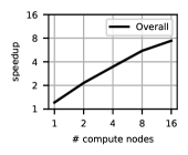
(a) Parallel speedup of epoch-based MPI algorithm over state-of-the-art shared-memory algorithm.

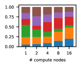
(b) Breakdown of running time. From bottom to top: diameter (blue), calibration (orange), epoch transition (green), non-blocking ibarrier (red), blocking MPI reduction (violet), check of stopping condition (brown).

Figure 2: Parallel scalability on real-world graphs

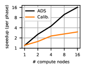
(a) Parallel speedup of epoch-based MPI algorithm over state-of-the-art shared-memory algorithm in adaptive sampling and calibration phases.

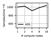
(b) Parallel scalability of epoch-based MPI algorithm in terms of samples per time and compute node.

Figure 3: Performance characteristics on real-world-graphs

In a first experiment, we evaluate the performance of our epoch-based MPI parallelization for betweenness approximation on the real-world instances of Table V-A. In absence of prior MPI-parallel approximation algorithms for betweenness, we compare our MPI-parallel code with the state-of-the-art shared-memory algorithm from Ref. [24]. Figure 1(a) depicts the speedup over this competitor. Our MPI parallelization achives an almost linear speedup for $P\leq 8$. For higher numbers of compute nodes, the sequential part of the computation takes a non-negligible fraction of the running time. This can be seen from Figure 1(b), which breaks down the fraction of time spent in different phases of the algorithm: indeed, the sequential diameter computation and sequential parts of the calibration phase become more signifiant for $P\geq 8$ (blue + orange bars). Note that the epoch transition and non-blocking barrier (green + red bars) are overlapped communication and computation, while the aggregation (violet bar) is the only non-overlapped communication done by the algorithm.

In Figure 2(a), we present the speedup during the adaptive sampling and calibration phases individually. Indeed, if we only consider the adaptive sampling phase, the algorithm scales well to all 16 compute nodes. While the sampling part of the calibration phase is pleasingly parrallel, for higher numbers of compute nodes, the sequential computations required for calibration dominate the running time of the calibration phase. Figure 2(b) analyzes the behavior during the adaptive sampling phase in more detail. This figure demonstrates that the sampling performance scales linearly during the adaptive sampling phase, regardless of the number of compute nodes. This is made possible by the fact that almost all communcation is overlapped by sampling.

TABLE II: Per-instance statistics on 16 compute nodes, including number of epochs (Ep.), samples taken by the algorithm before termination, seconds spent in non-blocking ibarrier (B), total communication volume in MiB per epoch (Com.), seconds spent in adaptive sampling (Time).

Finally, in Table V-B, we report per-instance statistics of the algorithm when all 16 compute nodes are used. The road networks require the highest amount of samples but the lowest amount communication per epoch (due to their small size). The algorithm consequently iterates through many epochs to solve the instance. The largest instances (in particular friendster and dimacs10-uk-2007-05) are solved within only two epochs since the samples collected during the first global barrier and aggregation are enough for KADABRA to terminate. Again, overlapping the communication and computation indeed allows the algorithm to be efficient even for large communication volumes per epoch.

V-C Scalability w. r. t. Graph Size

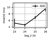
(a) R-MAT graphs

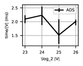
(b) Random hyperbolic graphs

Figure 4: Adaptive sampling time in relation to graph size on synthetic graphs

In the next experiment, we evaluate the epoch-based MPI algorithm’s ability to scale with the graph size. This experiment is performed on synthetic R-MAT and random hyperbolic graphs. We vary the number of vertices between $2^{23}$ and $2^{26}$ (resulting in between $250$ million and $2$ billion edges). Figure 4 reports the results in terms of time required for the adaptive sampling phase in relation to the graph size. On R-MAT graphs, the algorithm’s running time grows slightly superlinearly: the largest graphs require $1.85\times$ more time per vertex than the smaller graphs. On hyperbolic graphs, the performance is mostly unaffected by the graph size, so that we conclude that the algorithm scales linearly with the size of these graphs.

VI Conclusions

In this paper, we presented the first MPI-based parallelization of the state-of-the-art betweenness approximation algorithm KADABRA. Our parallelization is based on the epoch-based framework and non-blocking MPI collectives. Both techniques allow us to efficiently overlap communication and computation, which is the key challenge for parallelizing adaptive sampling algorithms. As a result, our algorithm is the first to allow the approximation of betweenness on complex networks with multiple billions of edges in less than ten minutes at an accuracy of $\epsilon=0.001$.

In future work, we would like to apply our method to other adaptive sampling algorithms. As mentioned before, we expect the necessary changes to be small.

References

- [1] Amir Abboud, Fabrizio Grandoni, and Virginia Vassilevska Williams. Subcubic equivalences between graph centrality problems, APSP and diameter. In SODA, pages 1681–1697. SIAM, 2015.
- [2] Ziyad AlGhamdi, Fuad Jamour, Spiros Skiadopoulos, and Panos Kalnis. A benchmark for betweenness centrality approximation algorithms on large graphs. In Proceedings of the 29th International Conference on Scientific and Statistical Database Management, SSDBM ’17, pages 6:1–6:12, New York, NY, USA, 2017. ACM.
- [3] David A Bader, Shiva Kintali, Kamesh Madduri, and Milena Mihail. Approximating betweenness centrality. In International Workshop on Algorithms and Models for the Web-Graph, pages 124–137. Springer, 2007.
- [4] David A. Bader, Henning Meyerhenke, Peter Sanders, and Dorothea Wagner, editors. Graph Partitioning and Graph Clustering, 10th DIMACS Implementation Challenge Workshop, Georgia Institute of Technology, Atlanta, GA, USA, February 13-14, 2012. Proceedings, volume 588 of Contemporary Mathematics. American Mathematical Society, 2013.
- [5] Massimo Bernaschi, Giancarlo Carbone, and Flavio Vella. Scalable betweenness centrality on multi-gpu systems. In Proceedings of the ACM International Conference on Computing Frontiers, CF ’16, pages 29–36, New York, NY, USA, 2016. ACM.
- [6] Michele Borassi, Pierluigi Crescenzi, Michel Habib, Walter A. Kosters, Andrea Marino, and Frank W. Takes. Fast diameter and radius bfs-based computation in (weakly connected) real-world graphs: With an application to the six degrees of separation games. Theor. Comput. Sci., 586:59–80, 2015.
- [7] Michele Borassi and Emanuele Natale. KADABRA is an adaptive algorithm for betweenness via random approximation. In ESA, volume 57 of LIPIcs, pages 20:1–20:18. Schloss Dagstuhl - Leibniz-Zentrum fuer Informatik, 2016.
- [8] Ulrik Brandes. A faster algorithm for betweenness centrality. The Journal of Mathematical Sociology, 25(2):163–177, 2001.
- [9] Ulrik Brandes and Christian Pich. Centrality estimation in large networks. International Journal of Bifurcation and Chaos, 17(07):2303–2318, 2007.
- [10] Camil Demetrescu, Andrew V. Goldberg, and David S. Johnson, editors. The Shortest Path Problem, Proceedings of a DIMACS Workshop, Piscataway, New Jersey, USA, November 13-14, 2006, volume 74 of DIMACS Series in Discrete Mathematics and Theoretical Computer Science. DIMACS/AMS, 2009.
- [11] Robert Geisberger, Peter Sanders, and Dominik Schultes. Better approximation of betweenness centrality. In Proceedings of the Meeting on Algorithm Engineering & Expermiments, pages 90–100. Society for Industrial and Applied Mathematics, 2008.
- [12] Loc Hoang, Matteo Pontecorvi, Roshan Dathathri, Gurbinder Gill, Bozhi You, Keshav Pingali, and Vijaya Ramachandran. A round-efficient distributed betweenness centrality algorithm. In PPoPP, pages 272–286, 2019.
- [13] Jérôme Kunegis. KONECT: the koblenz network collection. In WWW (Companion Volume), pages 1343–1350. International World Wide Web Conferences Steering Committee / ACM, 2013.
- [14] Jure Leskovec and Rok Sosic. SNAP: A general-purpose network analysis and graph-mining library. ACM TIST, 8(1):1:1–1:20, 2016.
- [15] Kamesh Madduri, David Ediger, Karl Jiang, David A. Bader, and Daniel G. Chavarría-Miranda. A faster parallel algorithm and efficient multithreaded implementations for evaluating betweenness centrality on massive datasets. In 23rd IEEE International Symposium on Parallel and Distributed Processing, IPDPS 2009, Rome, Italy, May 23-29, 2009, pages 1–8. IEEE, 2009.
- [16] John Matta, Gunes Ercal, and Koushik Sinha. Comparing the speed and accuracy of approaches to betweenness centrality approximation. Computational Social Networks, 6(1):2, Feb 2019.
- [17] Adam McLaughlin and David A. Bader. Accelerating gpu betweenness centrality. Commun. ACM, 61(8):85–92, July 2018.
- [18] Matteo Riondato and Evgenios M Kornaropoulos. Fast approximation of betweenness centrality through sampling. Data Mining and Knowledge Discovery, 30(2):438–475, 2016.
- [19] Matteo Riondato and Eli Upfal. Abra: Approximating betweenness centrality in static and dynamic graphs with rademacher averages. ACM Transactions on Knowledge Discovery from Data (TKDD), 12(5):61, 2018.
- [20] Ahmet Erdem Sariyüce, Kamer Kaya, Erik Saule, and Ümit V. Çatalyürek. Graph manipulations for fast centrality computation. TKDD, 11(3):26:1–26:25, 2017.
- [21] Ahmet Erdem Sariyüce, Kamer Kaya, Erik Saule, and Ümit V. Çatalyürek. Betweenness centrality on gpus and heterogeneous architectures. In Proceedings of the 6th Workshop on General Purpose Processor Using Graphics Processing Units, GPGPU-6, pages 76–85, New York, NY, USA, 2013. ACM.
- [22] Edgar Solomonik, Maciej Besta, Flavio Vella, and Torsten Hoefler. Scaling betweenness centrality using communication-efficient sparse matrix multiplication. In Proceedings of the International Conference for High Performance Computing, Networking, Storage and Analysis, SC ’17, pages 47:1–47:14, New York, NY, USA, 2017. ACM.
- [23] Christian L. Staudt, Aleksejs Sazonovs, and Henning Meyerhenke. Networkit: A tool suite for large-scale complex network analysis. Network Science, 4(4):508–530, 2016.
- [24] Alexander van der Grinten, Eugenio Angriman, and Henning Meyerhenke. Parallel adaptive sampling with almost no synchronization. In Euro-Par, volume 11725 of Lecture Notes in Computer Science, pages 434–447. Springer, 2019.