Level crossings and new exact solutions of the two-photon Rabi model

Abstract

An infinite family of exact solutions of the two-photon Rabi model was found by investigating the differential algebraic properties of the Hamiltonian. This family corresponds to energy level crossings not covered by the Juddian class, which is given by elemetary functions. In contrast, the new states are expressible in terms of parabolic cylinder or Bessel functions. We discuss three approaches for discovering this hidden structure: factorization of differential equations, Kimura transformation, and a doubly-infinite, transcendental basis of the Bargmann space.

I Formulation of the problem

Emary and Bishop were the first to describe exact solutions of the two-photon Rabi model Emary:02:: . They related them to crossings of energy levels with different parities of corresponding eigenfunctions. These exact solutions are expresible in terms of elementary functions are called the Juddian solutions. Moreover, Emary and Bishop noticed that their result describes only a part of the level-crossings which are clearly visible in a numerically obtained spectrum, and conjectured that the remaining level-crossings also correspond to exact solutions. This conjecture can be reformulated as the problem of full description of degenerate states in the 2-photon Rabi model. Our aim is to give a complete solution of this problem and to show that Emary and Bishop’s conjecture is true. We give explicit analytic formulae for eigenfunctions corresponding to level crossings which were conjectured by Emary and Bishop. More importantly, we show that they are of different nature and analytical properties that those found in Emary:02:: . The proposed method is general, it can be applied to arbitrary systems for which the Schödringer equation has order greater than two.

The two photon Rabi model is given by the following Hamiltonian

$$H=\omega a^{{\dagger}}a+\frac{\omega_{0}}{2}\sigma_{z}+2g\left[(a^{{\dagger}})^{2}+(a)^{2}\right]\sigma_{x}.$$ (1)

It is also known as the two-photon Jaynes-Cummings model investigated initially in Gerry:88:: , and with a view to population inversion in Penna:16:: . This is a phenomenological model of the two-photon interaction. Its RWA version was introduced in Sukumar:81:: . The reader can find a nice discussion and justification of the derivation in Emary:01:: .

For very recent studies of the two-photon Rabi model we refer the reader to JPA16 ; JPA17 , where a detailed references for this subject can be found.

In further consideration it is convenient to apply a unitary transformation $\widetilde{H}=U^{\dagger}HU$ with $U=(\sigma_{x}+\sigma_{z})/\sqrt{2}$. It gives

$$\begin{split}\widetilde{H}&=\omega a^{{\dagger}}a+\frac{\omega_{0}}{2}\sigma_{x}+2g\left[(a^{{\dagger}})^{2}+a^{2}\right]\sigma_{z}\\ &=2g\left\{2xa^{{\dagger}}a+\mu\sigma_{x}+\left[(a^{{\dagger}})^{2}+a^{2}\right]\sigma_{z}\right\},\end{split}$$ (2)

where we set $\omega=4xg$, and $\omega_{0}=4\mu g$. The rescaled Hamiltonian in matrix form reads

$$K :=\frac{1}{2g}\widetilde{H}=2xa^{{\dagger}}a+\mu\sigma_{x}+\left[(a^{{\dagger}})^{2}+a^{2}\right]\sigma_{z}$$ (3)

$$=\begin{bmatrix}2xa^{{\dagger}}a+\left[(a^{{\dagger}})^{2}+a^{2}\right]&\mu\\ \mu&2xa^{{\dagger}}a-\left[(a^{{\dagger}})^{2}+a^{2}\right]\end{bmatrix}.$$

We next employ the Bargmann representation, in which the state is a two-component spinor: $\psi\in\mathcal{H}^{2}$, where $\mathcal{H}$ is the Hilbert space which is a proper $\mathbb{C}$-linear subspace of entire functions $\mathscr{O}(\mathbb{C})$ of the complex variable $z\in\mathbb{C}$, with the scalar product

$$\langle f,g\rangle=\dfrac{1}{\pi}\int_{\mathbb{C}}\overline{f(z)}g(z)e^{-|z|^{2}}\mathrm{d}(\Re(z))\mathrm{d}(\Im(z)).$$ (4)

The operators $a^{{\dagger}}$ and $a$ become $z$ and $\partial_{z}$, respectively, so the stationary Schrödinger equation $K\psi=E\psi$, has the form of the following system of differential equations

$$\psi_{1}^{\prime\prime}(z)+2xz\psi_{1}^{\prime}(z)+(z^{2}-E)\psi_{1}(z)+\mu\psi_{2}(z) =0,$$ (5)

$$\psi_{2}^{\prime\prime}(z)-2xz\psi_{2}^{\prime}(z)+(z^{2}+E)\psi_{2}(z)-\mu\psi_{1}(z) =0.$$

In some calculations it is more convenient not to take the above system, but rather the corresponding fourth-order equation, obtained by elimination of $\psi_{2}$,

$$\varphi^{(\text{iv})}+((2-4x^{2})z^{2}+4x)\varphi^{\prime\prime}+4z(1+Ex-x^{2})\varphi^{\prime}+(2-E^{2}+\mu^{2}-4xz^{2}+z^{4})\varphi=0,$$ (6)

where we denote $\varphi(z)=\psi_{1}(z)$; written as $L_{2p}(\varphi)=0$, the equation defines the differential operator $L_{2p}$. As we showed in Maciejewski:17:: , the natural parameters of the problem are $\kappa$ and $\chi$ which are defined by relations

$$x=\frac{1}{2}\left(\frac{1}{\kappa}+\kappa\right)\qquad E=2\left(\frac{1}{\kappa}-\kappa\right)(\chi-1)-\kappa,$$ (7)

and $\chi$ is the spectral parameter. Here we assume that $\kappa\in(0,1)$ and $E>-1$. These restriction of parameters implies that $\chi\geq 1$. For justification of this parametrisation see our article Maciejewski:17:: .

For any fixed values of the parameters equation (6) has four linearly independent solution $\varphi_{i}(z)$, $i=1,\ldots,4$ which are entire functions. They are uniquely determined by four linearly independent initial conditions $(\varphi_{i}(z_{0}),\varphi_{i}^{\prime}(z_{0}),\varphi_{i}^{\prime\prime}(z_{0}),\varphi_{i}^{\prime\prime\prime}(z_{0}))$, $i=1,\ldots,4$, given for an arbitrary $z_{0}\in\mathbb{C}$. The fundamental problem is to decide if at least one of these solutions has a finite norm, i.e., whether a fixed value of $E$ (or $\chi)$ is the eigenvalue for which one or more solutions of (6) are eigenstates. Thus, potentially, the degeneracy of a given eigenvalue can be four. However, this bound cannot be achieved, and we claim that the degeneracy of eigenvalues is not higher than two.

To show this, let us recall that if an entire function belongs to Bargmann’s Hilbert space, then it has a proper growth order as $\lvert z\rvert\rightarrow\infty$. This growth is characterized by two numbers $(\rho,\sigma)$, the order $\rho$ and the type $\sigma$. Roughly speaking, $f(z)$ has order $\rho$ and type $\sigma$ if $\lvert f(z)\rvert$ behaves as $\exp\left(\sigma\lvert z\rvert^{\rho}\right)$ for large $\lvert z\rvert$, see Vourdas:06:: . It can be shown that if $f(z)$ has a finite norm then $\rho\leq 2$ and $\sigma\leq 1/2$.

Equation (6) has an irregular singular point at infinity. Formal solutions $\widehat{\varphi}(z)$ near this point give us information about the asymptotics of all solutions for large $\lvert z\rvert$. The basis $\widehat{\varphi}_{i}(z)$ with $i=1,\ldots,4$ of formal solutions of equation (6) is the following:

$$\begin{split}\widehat{\varphi}_{1}(z)=z^{-1/2}\exp\left[\frac{\kappa}{2}z^{2}\right]\left(1+\mathscr{O}(z^{-2})\right),&\quad\widehat{\varphi}_{2}(z)=z^{-3/2}\exp\left[-\frac{\kappa}{2}z^{2}\right]\left(1+\mathscr{O}(z^{-2})\right),\\ \widehat{\varphi}_{3}(z)=z^{-9/2}\exp\left[\frac{1}{2\kappa}z^{2}\right]\left(1+\mathscr{O}(z^{-2})\right),&\quad\widehat{\varphi}_{4}(z)=z^{-5/2}\exp\left[-\frac{1}{2\kappa}z^{2}\right]\left(1+\mathscr{O}(z^{-2})\right).\end{split}$$ (8)

The above expansions are asymptotic to true solutions $\varphi_{i}(z)$ only in a narrow enough sector of the complex plane. From their form it follows that all solutions of equation (6) have order $\rho=2$. However, a changing of the sector permutes these asymptotic expansions and this is the effect of the Stokes phenomenon, see Wasow . This is why generic solutions have the maximal type which in our case is $1/2\kappa>1/2$. The above shows that there are at most two linearly independent solutions of type $\sigma=\kappa/2<1/2$. For if there existed a solution independent of $\hat{\varphi}_{1}$ and $\hat{\varphi}_{2}$, but with the type different from $\hat{\varphi}_{3}$ and $\hat{\varphi}_{4}$, the basis would have 5 elements, by the correspondence between formal and global bases Wasow . Thus, we arrive at

Observation 1

The degeneracy in the two-photon Rabi model is at most two.

In any case, the condition that a solution of equation (6) is an eigenvector puts restrictions on the Stokes matrices which are highly transcendental objects.

The two photon Rabi model described by Hamiltonian (3) has a $\mathbb{Z}_{4}$ symmetry. The Hamiltonian $K$ commutes with the operator $\tau$ defined as

$$\tau\psi(z)=\sigma_{x}\psi(\mathrm{i}z),\qquad\psi=(\psi_{1},\psi_{2})^{T},\quad\sigma_{x}=\begin{bmatrix}0&1\\ 1&0\end{bmatrix}$$ (9)

The associated symmetry group is $\mathbb{Z}_{4}$ isomorphic to $\{1,\tau,\tau^{2},\tau^{3}\}$.

The basis of the solutions space of (6) has four elements, and they can be numbered according to their $\mathbb{Z}_{4}$ parity. For a solution with parity $s$ one has $\tau\psi(z)=s\psi$, so

$$\begin{split}\psi_{1}(\mathrm{i}z)&=s\psi_{2}(z),\\ \psi_{2}(\mathrm{i}z)&=s\psi_{1}(z),\end{split}$$ (10)

where $s\in\{+1,-1,\mathrm{i},-\mathrm{i}\}$. Because $\tau^{2}\psi(z)=\psi(-z)$, the distinction between even and odd solutions represents the $\mathbb{Z}_{2}$ subgroup of the symmetry and can be used to simplify the calculation.

We can distinguish four linearly independent solutions of system (6): $\psi^{(s)}=(\psi_{1}^{(s)},\psi_{2}^{(s)})$ with $s\in\{+1,-1,\mathrm{i},-\mathrm{i}\}$ just specifying initial conditions $(\psi^{(s)}(0),{\psi^{(s)}}^{\prime}(0))$. A simple reasoning shows that if $s\in\{-1,+1\}$ then $\psi^{(s)}(0)=(1,s)$ and ${\psi^{(s)}}^{\prime}(0)=(0,0)$. In this case $\psi^{(s)}(z)=\psi^{(s)}(-z)$. If $s\in\{\mathrm{i},-\mathrm{i}\}$, then $\psi^{(s)}(0)=(0,0)$ and ${\psi^{(s)}}^{\prime}(0)=(1,-\mathrm{i}s)$; in this case $\psi^{(s)}(z)=-\psi^{(s)}(-z)$. Clearly, these four initial conditions are linearly independent. Each solution $\psi(z)$ of system (6) is a linear combination

$$\psi(z)=c_{-1}\psi^{(-1)}(z)+c_{+1}\psi^{(+1)}(z)+c_{-\mathrm{i}}\psi^{(-\mathrm{i})}(z)+c_{+\mathrm{i}}\psi^{(+\mathrm{i})}(z).$$ (11)

In other words, for a specific energy $E$, once the parity $s$ is fixed, so are the initial conditions at $z=0$, and the state is uniquely determined up to a multiplicative constant.

The spectrum of the two-photon Rabi model is shown in Figure 1. The color of a curve marks the parity of the corresponding eigenfunction: green, blue, red and orange for $+1$, $-1$, $+\mathrm{i}$ and $-\mathrm{i}$, respectively. The Judd states correspond to crossings at levels $\chi=n/2$, with integer $n>1$. They occur only as intersections of two curves with parities $(+1,-1)$ or $(+\mathrm{i},-\mathrm{i})$. The intersections marked with circles correspond to new states discussed in this papers. For them there are four admissibly parities of intersecting curves $(\pm 1,\pm\mathrm{i})$. Values of $\chi$ for these crossings are $\chi=(2\ell+3)/4$ for integer $\ell\geq 1$. This fact is not trivial as the curves are know only numerically. In fact, at first we determined these values of $\chi$ investing continued fractions of successive numerical approximations. Later we show how these distinguished values of $\chi$ naturally appear in our approach.

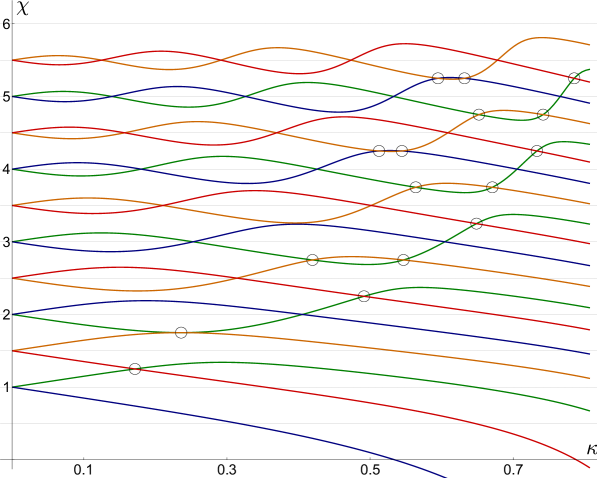
Figure 1: Spectrum of the two-photon Rabi model for $\mu=3$, parities: blue: $-1$, green: $+1$, red: $-\text{i}$, orange: $+\text{i}$. Circles indicate the new states; the remaining crossings are Juddian.

In the next section we describe the main idea of our approach to the problem. The eigenvectors corresponding to special points of the spectrum are distinguished by their analytical form: for Judd states they are given by elementary function while for the remaining ones – by higher transcendental functions (Bessel, or parabolic cylinder). The reason why this simplification occurs is connected to an algebraic property of the differential operator defined by the stationary Schrödinger equation. Physical manifestation of this property is the degeneracy of the spectrum, and the main result can be summarized as follows:

Observation 2

Degeneracy in the two-photon Rabi model occurs when $\chi=m/4$, with $m\in\mathbb{Z}_{+}$, and the Schroedinger equation is factorizable. Juddian solutions appear for even $m$, and in this case the equation has a 1st order factor; for odd $m=2\ell+3$, $\ell\in\mathbb{Z}_{+}$, the minimal factor is of 2nd order, and for each $\ell$ the degenerate eigenstates are given by classical transcendental functions by formula (38); the appropriate algebraic conditions on $\kappa$ and $\mu$ is given by the determinant of equations (42).

II Factorization

II.1 First approach

The exact solutions of the two-photon Rabi model found by Emary and Bishop  Emary:02:: correspond to $\chi=n/2$ , where $n$ is an integer, and are directly related to the Judd solutions of the standard Rabi model Emary:02:: in two ways. First, the solutions are exponential

$$\psi_{1}(z)=\mathrm{e}^{az^{2}}P(z),$$ (12)

where $P(z)$ is a polynomial, and $2a\in\{\pm\kappa,\pm\kappa^{-1}\}$. Second, they come about by degeneracy of energy levels with different parities. More precisely, the eigenspace of a Judd state is two dimensional and all eigenvectors $\psi(z)=(\psi_{1}(z),\psi_{2}(z))$ from this space are either even, when it appears as a level crossing of states with $\mathbb{Z}_{4}$ parities $+1$ and $-1$, or they are odd – for level crossing of states with parities , $+\mathrm{i}$ and $-\mathrm{i}$.

Moreover, from the mathematical point of view, what happens is that the differential equation (6) is reducible, i.e., the corresponding differential operator $L_{\mathrm{2p}}$ can be factorized

$$L_{\mathrm{2p}}=L_{3}L_{1}.$$ (13)

where $L_{1}$ is a first order differential operator. It seems that this fact was never mentioned in the literature in this context.

Knowing the above we asked if it is possible that the operator $L_{\mathrm{2p}}$ has a right factor of second order, and if so – what is the physical meaning of this kind of factorization?

Let us notice that if $L_{\mathrm{2p}}$ admits the factorization

$$L_{\mathrm{2p}}=\widetilde{L}_{2}L_{2},$$ (14)

then a solution of equation $L_{2}(y)=0$ is also a solution equation (6). Thus, the question is if there exist energies for which states are solutions of second order differential equations. We take the factor to be minimal, for if $L_{2}=\tilde{L}_{1}L_{1}$, we would be back in the previous case. In the mathematical literature functions which are solutions of a second order linear differential equations are called Eulerian, see Singer85 .

The problem of factorization of differential operator is a classical subject. A short exposition can be found in Bronstein:94:: . Using the algorithm and facts from this reference it can be shown that:

1. if the differential operator $L_{\mathrm{2p}}$ has a right second-order factor $L_{2}$, then

   $$\chi=\frac{2\ell+3}{4},\qquad\ell\in\mathbb{Z};$$ (15)

2. the remaining parameters satisfy the algebraic condition $P_{\ell}(\mu,\kappa)P_{\ell}(-\mu,\kappa)=0$. where $P_{\ell}(x,y)\in\mathbb{Z}[x,y]$ is a polynomial with integer coefficients;

3. for $\ell>0$ all solutions of the right factor $L_{2}(\psi_{1})=0$ have a finite Bargmann norm; for $\ell\leq 0$ these solutions are not normalizable;

For $\ell=1$, i.e., for $\chi=5/4$, the right factor $L_{2}$ of $L_{\mathrm{2p}}$ is given by

$$L_{2}=\partial_{z}^{2}+\kappa(2-\kappa z^{2}),$$ (16)

The algebraic restriction for the other parameters is given by the polynomial $P_{1}(\mu,\kappa)=(2\mu\kappa+\kappa^{2}+1)$. It is important to remark here that an arbitrary solution $V(z)$ of the equation $L_{2}(V)=0$ has finite norm. In fact, the equation

$$L_{2}(V)=V^{\prime\prime}(z)+\kappa(2-\kappa z^{2})V(z)=0$$ (17)

has only one irregular singular point at infinity so all its solutions are entire functions. Moreover, the basis of formal solutions near infinity is

$$\widehat{V}_{1}(z)=z^{1/2}\mathrm{e}^{-\frac{\kappa}{2}z^{2}}\left(1+O(z^{-2})\right),\quad\widehat{V}_{2}(z)=z^{-3/2}\mathrm{e}^{\frac{\kappa}{2}z^{2}}\left(1+O(z^{-2})\right),\quad$$ (18)

An entire function $V(z)$ with these asymptotics has order $2$ and type $\kappa/2$. As $\kappa\in(0,1)$, the Bargmann norm of $V(z)$ is finite. Two linearly independent solution of (17) are

$$V_{1}(z)=D_{1/2}(\sqrt{2\kappa}z),\qquad V_{2}(z)=D_{1/2}(-\sqrt{2\kappa}z)$$ (19)

where $D_{n}(z)$ denotes the parabolic cylinder function in Whittaker’s convention, see (Whittaker and Watson, 1935, §16.5); for a compilation of definitions, conventions and properties see DLMF . These two functions form a basis of the eigenspace for $\chi=5/4$, i.e.,

$$\psi_{1}(z)=c_{1}D_{1/2}(\sqrt{2\kappa}z)+c_{2}D_{1/2}(-\sqrt{2\kappa}z)$$

where $c_{1}$ and $c_{2}$ are arbitrary constants.

For $\ell=2$ the right factor of $L_{2\mathrm{p}}$ is

$$L_{2}=\partial_{z}^{2}+b_{1}(z)\partial_{z}+b_{0},$$ (20)

where

$$b_{1}(z)=-\frac{2(1+\kappa^{2})z}{(1+\kappa^{2})z^{2}-2\kappa}$$ (21)

$$b_{0}(z)=2\kappa-\kappa^{2}z^{2}+\frac{9-2(11+2\mu^{2})\kappa^{2}+\kappa^{4}}{4(1-\kappa^{2})\left[(1+\kappa^{2})z^{2}-2\kappa\right]}.$$ (22)

The algebraic restrictions are given by the polynomial

$$P_{2}(\mu,\kappa)=3(1+\kappa^{2})^{2}-8\mu\kappa(1-\kappa^{2})+4\mu^{2}\kappa^{2}.$$ (23)

Let us notice that now the differential equation $L_{2}(V)=0$ has regular singularities at points

$$z_{\pm}=\pm\sqrt{\frac{2\kappa}{1+\kappa^{2}}}.$$ (24)

The differences of exponents at these points are both equal 2 but nevertheless all its solutions are entire. The algebraic condition $P_{2}(\mu,\kappa)P_{2}(-\mu,\kappa)=0$ guarantees a that $L_{2}$ is the right factor of $L_{2\mathrm{p}}$, and this in turn implies the logarithmic therms are not present in the solutions of $L_{2}(V)=0$. Quite amazingly, the basis of formal solution of $L_{2}(V)=0$ near infinity is the same as for the respective equation for $\ell=1$, that is it has the form (18). We postpone giving explicit solutions until the next two section, where different values of $\ell$ can be treated together.

Taking $\ell>2$ we obtain the right factor $L_{2}$ which is of the form (20) with rational $b_{1}(z)$ and $b_{0}(z)$. However, the number of regular singularities is $2(\ell-1)$, and the expressions obtained for the coefficients are quite complicated. For the regular singularities the differences of exponents are integers. However, the condition $P_{\ell}(\mu,\kappa)P_{\ell}(-\mu,\kappa)=0$ guarantees that all these singularity are apparent, see Barkatou:15:: . Thus, one would like to remove them by transforming the factor equation $L_{2}(V)=0$ into a second order equation without singular points in the finite part of the complex plane. This question reformulated in more general settings is not new. From the relevant theory Barkatou:15:: it follows that the answer to this question is generally negative, and known methods are not directly applicable for our problem. This is why we decided to modify our approach.

II.2 Second approach

Equation (6) has a second order factor if its solution space has a two dimensional subspace spanned by a basis of solutions of second order equation. The real problem is the dependence on parameters. We know that necessary condition for the factorization is $\ell\in\mathbb{Z}$. Let $\mathscr{W}_{\ell}$ denote the above mentioned subspace of solutions for $\ell>0$. Our crucial observation is that for each $\ell\in\mathbb{Z}$ if $V(z)\in\mathscr{W}_{\ell}$, then

$$V(z)=A_{\ell}(z)d(z)+B_{\ell}(z)d^{\prime}(z),$$ (25)

where $A_{\ell}(z)$, $B_{\ell}(z)$ are polynomials, and $d(z)$ is an arbitrary solution of the following differential equation

$$d^{\prime\prime}(z)+\kappa(2-\kappa z^{2})d(z)=0.$$ (26)

This kind of transformation often appears in the problem of removing apparent singularities, as introduced by Kimura in application to the hypergeometric equation Kimura:70:: .

Here it is important to underline that

1. $d(z)$ does not depend on $\ell$;

2. an arbitrary solution $d(z)$ of (26) has finite Bargmann norm (see below), so all elements of $\mathscr{W}_{\ell}$ have finite Bargmann norm;

3. the function $V(z)$ given by (25) is a solution of  (6) if and only if the condition $P_{\ell}(\mu,\kappa)P_{\ell}(-\mu,\kappa)=0$ is satisfied;

4. the polynomial $A_{\ell}(z)$ has degree $(\ell-1)$ and $A_{\ell}(-z)=(-1)^{\ell+1}A_{\ell}(z)$;

5. the polynomial $B_{\ell}(z)$ has degree $(\ell-2)$, $B_{2}(z)=0$ and $B_{\ell}(-z)=(-1)^{\ell}B_{\ell}(z)$.

Crucially, from the practical point of view, it is enough to assume that $\psi_{1}(z)=A(z)d(z)+B(z)d^{\prime}(z)$, where $A(z)$ and $B(z)$ are polynomials, is a solution of (6), and we can derive all the conclusions given above.

In the preceding section, the factors $L_{2}$ depended on $\ell$. Here, there is just the equation for $d(z)$ and all solutions will involve only two transcendental functions, i.e., the two independent solutions of (26). Recall that the classical Judd states are given by polynomials and exponentials – the latter being a solution of a first order differential equation, this means the solutions are Liouvillian. Here, by contrast, in addition to polynomials we have solutions of a second-order equation, that is to say: Eulerian functions. In this case they are the modified Bessel functions of the first kind, for we have

$$d^{(\pm)}(z)=z^{\frac{3}{2}}I_{\pm\frac{1}{4}}\left(\frac{\kappa}{2}z^{2}\right)-z^{\frac{3}{2}}I_{\mp\frac{3}{4}}\left(\frac{\kappa}{2}z^{2}\right).$$ (27)

The algebraic singularity is apparent, since the equation only admits entire solutions – the above can be analytically continued over the whole complex plane. The above form of solution appears naturally when the Laplace transformation is used for finding form (25). The basis $d^{\pm}(z)$ has prescribed symmetry as the notation suggests. Namely, equation (26) coincides with (17) and one can check that

$$d^{\pm}(z)=c_{\pm}\left[D_{1/2}(\sqrt{2\kappa}z)\pm D_{1/2}(-\sqrt{2\kappa}z)\right]$$ (28)

where $c_{\pm}$ are non-zero constants. In connection with the results of Dolya Dolya , one more representation of the general solution of (26) would be through the confluent hypergeometric function:

$$d(z)=c_{1}\text{e}^{-\frac{\kappa}{2}z^{2}}{}_{1}F_{1}\left(-\tfrac{1}{4},\tfrac{1}{2},\kappa z^{2}\right)+c_{2}z\text{e}^{-\frac{\kappa}{2}z^{2}}{}_{1}F_{1}\left(\tfrac{1}{4},\tfrac{3}{2},\kappa z^{2}\right).$$ (29)

For $\ell=1$ the solution becomes just

$$\psi_{1}=d(z).$$ (30)

For $\ell=2$ we have

$$\psi_{1}=\kappa\left(7-\kappa^{4}+\kappa^{2}(6+4\mu^{2})\right)zd(z)+\left(7\kappa^{4}+\kappa^{2}(6+4\mu^{2})-1\right)d^{\prime}(z).$$ (31)

For $\ell=3$ we have

$$\psi_{1}= \left(z^{2}+\tfrac{519\kappa^{8}-12(159+2\mu^{2})\kappa^{6}-2(1155+8\mu^{2}(31+\mu^{2}))\kappa^{4}+4(27+10\mu^{2})\kappa^{2}-9}{256\kappa(1-\kappa^{4})(1-\kappa^{2})^{2}}\right)d(z)+$$ (32)

$$\tfrac{\kappa^{2}(62+4\mu^{2})-1-\kappa^{4})}{16\kappa(1-\kappa^{2})^{2}}zd^{\prime}(z).$$

We deduced representation (25) partly in the process of removing apparent singularities with Kimura’s method, and partly by inspecting several examples. Clearly, it needs further mathematical investigation, which we attempt below.

II.3 Third approach

The third and final picture of the new solutions is a simplification of the previous representation, which uses one special function $d(z)$ and polynomial coefficients. Instead of finding coefficients of polynomials, as solutions of a differential equation, one might wish to construct a new basis in the Hilbert space, such that the solutions are simply finite linear combinations, rendering the problem equivalent to solving a linear system. To this end we introduce a new independent variable $\zeta=\sqrt{2\kappa}z$, and consider (26) generalized thus

$$\mathscr{D}_{n}^{\prime\prime}(\zeta)+\left(n+1-\tfrac{1}{4}\zeta^{2}\right)\mathscr{D}_{n}(\zeta)=0.$$ (33)

The previously used function corresponds to $n=0$ so that $d(z)=\mathscr{D}_{0}(\sqrt{2\kappa}z)$, and it is clear that $\mathscr{D}_{n}$ are entire functions for all $n$. The two independent solutions can be taken as $\mathscr{D}^{(\pm)}_{n}(\zeta):=D_{n+\frac{1}{2}}(\zeta)\pm D_{n+\frac{1}{2}}(-\zeta)$, where $D_{n}$ are the aforementioned parabolic cylindrical functions. In addition to the differential equation, the new functions satisfy the relations

$$\tfrac{1}{2}\zeta\mathscr{D}_{n}-\mathscr{D}_{n}^{\prime}=\mathscr{D}_{n+1},\quad\text{and}\quad\tfrac{1}{2}\zeta\mathscr{D}_{n}+\mathscr{D}_{n}^{\prime}=(n+\tfrac{1}{2})\mathscr{D}_{n-1},$$ (34)

so it makes sense to introduce the raising and lowering operators

$$\left.\begin{aligned} b^{{\dagger}}&:=\tfrac{1}{2}\zeta-\partial_{\zeta}\\ b&:=\tfrac{1}{2}\zeta+\partial_{\zeta}\end{aligned}\,\right\}\quad\Longrightarrow\quad\left\{\begin{aligned} b^{{\dagger}}\mathscr{D}_{n}&=\mathscr{D}_{n+1}\\ b\mathscr{D}_{n}&=\left(n+\tfrac{1}{2}\right)\mathscr{D}_{n-1}\end{aligned}\right.,$$ (35)

which obey $[b,b^{{\dagger}}]=1$. We use the conventional notation, but note that they are not Hermitian conjugates in the Bargmann product. What is more, unlike in the standard case, $\mathscr{D}_{0}$ is not annihilated by $b$, so we have a doubly infinite series, i.e., $n\in\mathbb{Z}$.

The triple $b^{{\dagger}}b$, $b^{2}$ and ${b^{{\dagger}}}^{2}$ satisfy the commutation relations of the $\mathfrak{su}(1,1)$ algebra

$$\left[b^{{\dagger}}b+\tfrac{1}{2},{b^{{\dagger}}}^{2}\right]=2{b^{{\dagger}}}^{2},\quad\left[b^{{\dagger}}b+\tfrac{1}{2},b^{2}\right]=-2b^{2},\quad\left[b^{2},{b^{{\dagger}}}^{2}\right]=4\left(b^{{\dagger}}b+\tfrac{1}{2}\right).$$ (36)

However, we cannot immediately choose one of the irreducible representations because here $b^{{\dagger}}$ does not denote the Hermitian conjugate of $b$. A further Lie algebraic analysis will be given in a separate publication, Here, we follow the direct path, which is simple enough in this case.

The Schrödinger equation (5) can now be written as

$$N\psi_{1}+\frac{1+\kappa^{2}}{1-\kappa^{2}}b^{2}\psi_{1}+(2-2\chi)\psi_{1}+\frac{\mu\kappa}{1-\kappa^{2}}\psi_{2} =0,$$ (37)

$$N\psi_{2}+\frac{1+\kappa^{2}}{1-\kappa^{2}}{b^{{\dagger}}}^{2}\psi_{2}-(1-2\chi)\psi_{2}-\frac{\mu\kappa}{1-\kappa^{2}}\psi_{1} =0,$$

where $N:=b^{{\dagger}}b$ so that $N\mathscr{D}_{n}=\left(n+\frac{1}{2}\right)\mathscr{D}_{n}$. As can be seen, all the involved operators, when applied to $\mathscr{D}_{n}$, shift the index by 0 or 2. We can thus look for solutions of the form

$$\psi_{1}=\sum_{j=0}^{l_{3}}a_{j}\mathscr{D}_{l_{1}+2j},\quad\psi_{2}=\sum_{j=0}^{l_{4}}c_{j}\mathscr{D}_{l_{2}+2j},$$ (38)

i.e., finite expansions in terms of entire functions like in (25), except this time the coefficients are constant, and there is more than one function $d(z)$.

The new parameters can be limited, by inspecting the terms with the lowest indices: in the first component of (37), $b^{2}\psi_{1}$ must cancel with $\psi_{2}$; in the second, ${b^{{\dagger}}}^{2}\psi_{2}$ must cancel with $\psi_{1}$. The two conditions are $l_{1}-2=l_{2}$, and $l_{2}+2l_{4}+2=l_{1}+2l_{3}$, or simply: $l_{4}=l_{3}$ and $l_{2}=l_{1}-2$. It then follows that the highest terms in the first equation come from $N\psi_{1}+(2-2\chi)\psi_{1}$, and the lowest in the second from $N\psi_{2}-(1-2\chi)\psi_{2}$, their cancellation requires that

$$\chi=\frac{3+2l_{3}}{4},\quad\text{and}\quad l_{1}=-1-l_{3}.$$ (39)

By (15), we recognize that $l_{3}=\ell$, so $\chi$ fully specifies the index ranges.

We are now ready to turn the Schrödinger equation into a homogeneous linear systems of equations for $a_{j}$ and $c_{j}$, with a tridiagonal structure. Indeed, the first equation in (37) is easily solved for $\psi_{2}$, and direct substitution changes the second one into $\mathscr{L}\psi_{1}=0$, where the operator $\mathscr{L}(N,b^{2},{b^{{\dagger}}}^{2})$ acts on $\mathscr{D}_{n}$ simply as $\mathscr{L}\mathscr{D}_{n}=\beta_{n}\mathscr{D}_{n}+\alpha_{n}\mathscr{D}_{n+2}+\gamma_{n}\mathscr{D}_{n-2}$ where

$$\alpha_{n} =(1-\kappa^{4})(5+2n-4\chi),$$ (40)

$$\beta_{n} =(1+\kappa^{4})(4n^{2}-1)+2(1-\kappa^{2})^{2}(2n-1-2\chi(2\chi-3))+2\kappa^{2}\mu^{2},$$

$$\gamma_{n} =(1-\kappa^{4})(n^{2}-\tfrac{1}{4})(4\chi+2n-5).$$

With the substitution (38), the remaining equation becomes $\mathscr{L}\sum a_{n}\mathscr{D}_{l_{1}+2n}=0$, or, by independence of $\mathscr{D}_{n}$, a set of recurrence relations

$$\alpha_{l_{1}+2n-2}a_{n-1}+\beta_{l_{1}+2n}a_{n}+\gamma_{l_{1}+2n+2}a_{n+1}=0,\qquad n=0,\ldots,\ell;$$ (41)

the equivalent system reads

$$\begin{bmatrix}\beta_{-\ell-1}&\gamma_{-\ell+1}&&&&\\ \alpha_{-\ell-1}&\beta_{-\ell+1}&\gamma_{-\ell+3}&&\scalebox{1.5}{0}&\\ &\alpha_{-\ell+1}&\ddots&\ddots&&\\ &&\ddots&\ddots&\gamma_{\ell-3}&\\ &\scalebox{1.5}{0}&&\alpha_{\ell-5}&\beta_{\ell-3}&\gamma_{\ell-1}\\ &&&&\alpha_{\ell-3}&\beta_{\ell-1}\end{bmatrix}\begin{bmatrix}a_{0}\\ a_{1}\\ a_{2}\\ \vdots\\ a_{\ell-1}\\ a_{\ell}\end{bmatrix}=0,$$ (42)

which is of finite size $\ell+1$ by assumption. For a non-zero solution, the main determinant must vanish – it turns out to be exactly the algebraic condition $P_{\ell}(\mu,\kappa)P_{\ell}(-\mu,\kappa)=0$. Since $\mathscr{D}_{n}$ could be any of the basis solutions, we have obtained solutions for both parities: as $\tau^{2}\psi(z)=\psi(-z)=s^{2}\psi(z)$, the parity of $\mathscr{D}^{(+)}$ is in $\{1,-1\}$, while that of $\mathscr{D}^{(-)}$ belongs to $\{\mathrm{i},-\mathrm{i}\}$. We thus have “cross” degeneracy. To determine $s$ specifically one can use the connection formula

$$\mathscr{D}_{n}(\mathrm{i}\zeta)=\frac{\mathrm{i}\,\Gamma\!\left(n+\tfrac{3}{2}\right)}{\sqrt{2\pi}}\left[\mathrm{i}^{n-\frac{1}{2}}\mathscr{D}_{-n-2}(-\zeta)-\mathrm{i}^{\frac{1}{2}-n}\mathscr{D}_{-n-2}(\zeta)\right],$$ (43)

and check the quantity $\psi_{1}(\text{i}z)/\psi_{2}(z)$. Another option is to check the expansion of $\psi$ around zero, once the coefficients of (38) have been solved for, and compare with those in Section I.

The full solutions for $\chi=\frac{5}{4}$ are

$$\psi_{1}=\mathscr{D}_{0},\quad\psi_{2}=\frac{1+\kappa^{2}}{\mu\kappa}\mathscr{D}_{-2},$$ (44)

where $\mathscr{D}$ of the same parity should be taken in both components.

Likewise, solutions for $\chi=\frac{7}{4}$ read

$$\psi_{1} =\frac{8\kappa^{2}(1-\kappa^{2})\mu^{2}}{(1+\kappa^{2})(3+3\kappa^{4}+\kappa^{2}(6+4\mu^{2}))}\mathscr{D}_{-1}+\mathscr{D}_{1},$$ (45)

$$\psi_{2} =\frac{6\kappa(\kappa^{2}-1)\mu}{3+3\kappa^{4}+\kappa^{2}(6+4\mu^{2})}\mathscr{D}_{-3}+\frac{\kappa\mu}{1+\kappa^{2}}\mathscr{D}_{-1}.$$

Getting back to the previous representation is also straightforward, due to the recurrence relation

$$\zeta\mathscr{D}_{n}=\left(n+\tfrac{1}{2}\right)\mathscr{D}_{n-1}+\mathscr{D}_{n+1},$$ (46)

which allows us to reduce all $\mathscr{D}_{n}$ to a combination of $\mathscr{D}_{0}$ and $\mathscr{D}_{1}$. This comes at the price of generating polynomials of $\zeta$ as coefficients. $\mathscr{D}_{1}$ can then be changed to $\mathscr{D}_{0}^{\prime}$ using (35), and we are back to the $V=Ad+Bd^{\prime}$ form.

By extension, the recurrence relations allow us to manipulate the Bessel functions of (27), and the solutions can be expressed as a sum of $I_{\nu}$ of quarter order $\nu\in\frac{1}{4}+\mathbb{Z}$. This is another reason for adoption of $\chi$ as a natural parameter – quarters correspond to the newly found states, while half integer values (for which the Bessel function reduce to exponentials) correspond to those of Emary and Bishop. The relation of Juddian states to elementary Bessel functions was also the basis of Reik’s approach Reik .

III Symmetry and degeneracy

As we already mentioned, the Hamiltonian $K$ of the two-photon Rabi model commutes with the symmetry operator $\tau$ defined by (9). Thus, if $H\psi=E\psi$, then $H\tau(\psi)=E\tau(\psi)$. Hence

• if $\psi$ is an eigenstate for given energy than also $\tau(\psi)$, $\tau^{2}(\psi)$, $\tau^{3}(\psi)$, are eigenstate for this energy.

• if $\mathscr{W}_{E}$ is eigenspace corresponding to energy $E$ then it is spanned by eigenvectors of $\tau$

In particular, if energy $E$ is not degenerate, then necessarily $\tau(\psi)=s\psi$ with $s\in\{+1,-1,\mathrm{i},-\mathrm{i}\}$. In other words, non-degenerate eigenstates have specified parity with respect to $\mathbb{Z}_{4}$ symmetry.

If energy $E$ is degenerate, then we know that $\mathscr{W}_{E}$ has dimension two, so it is spanned by two eigenstates $\psi_{(r)}$ and $\psi_{(s)}$ with $r,s\in\{+1,-1,\mathrm{i},-\mathrm{i}\}$, $r\neq s$, which satisfy $\tau(\psi_{(r)})=r\psi_{(r)}$, $\tau(\psi_{(s)})=s\psi_{(s)}$. There are four unordered pairs $(r,s)$ of parities $(1,-1)$, $(1,\mathrm{i})$, $(1,-\mathrm{i})$, and $(\mathrm{i},-\mathrm{i})$.

The Judd type states found by Emary and Bishop correspond to pairs $(r,s)=(1,-1)$ and $(\mathrm{i},-\mathrm{i})$. In the first case $\mathscr{W}_{E}$ is spanned by states which are even functions, while in the second case $\mathscr{W}_{E}$ is spanned by odd states. Thus the Judd type states of Emary and Bishop have fixed $\mathbb{Z}_{2}$ parities corresponding to $\tau^{2}$.

IV Conclusions and remarks

In this article we investigated degenerate states of the two-photon Rabi model. One part of the collection of such states, called the Judd type states, was discovered by Emary and Bishop in Emary:02:: . The spinors are given by simple elementary functions. We observe that this fact is a consequence of factorisation of the stationary Schrödinger equation, which, in Bargmann’s representation, has the form of a fourth order differential equations. The existence of the other part of the degenerate spectrum was a conjecture Emary:02:: . We proved this conjecture, and found the analytical form of the eigenstates and energies.

Our main idea was that degenerate eigenstates have simpler analytical form than those nondegenerate, because they are the solutions of a differential equation of order lower than the order of the Schrödinger equation. We determined the asymptotics of the solutions, and showed that the degeneracy can at most be two-fold. The resulting two-dimensional eigenspaces are spanned by states with two different $\mathbb{Z}_{4}$ parities.

The existence of such a lower-order equation in those subspaces means that the Schrödinger equation considered as a differential operator has a right factor. We showed that the remaining part of the degenerate spectrum corresponds to the case when this factor has order two, so the eigenstates are given explicitly by solutions of second order differential equations and higher transcendental functions (equivalently by parabolic cylinder, Bessel or confluent hypergeometric).

The factorisation method for differential operators is well known in the context of quantum mechanics, see eg. book Dong:07:: . However, standard techniques consist of factorisation of the Hamiltonian – here, in contrast, we factorised the operator corresponding to the whole Schrödinger equation.

In the article Dolya , partially overlapping with our analysis, Dolya investigated quasiexact solvability of the two-photon Rabi system, and obtained similar expressions for eigenstates given by confluent hypergeometric functions, however this result was discarded in Yao:13:: .

References

- (1) Barkatou, Moulay A. and Maddah, Suzy S., Removing Apparent Singularities of Systems of Linear Differential Equations with Rational Function Coefficients, ISSAC 2015 - International Symposium on Symbolic and Algebraic Computation, Proceedings of the 2015 ACM on International Symposium on Symbolic and Algebraic Computation, 2015, pp. 53-60.
- (2) M. Bronstein, An improved algorithm for factoring linear ordinary differential operators. In Proceedings of the international symposium on Symbolic and algebraic computation (ISSAC ’94). ACM, New York, NY, USA, 1994, pp. 336-340.
- (3) Dong, S.-H., Factorization Method in Quantum Mechanics. Springer Science & Business Media, 2007
- (4) C. Gerry, Two-photon Jaynes-Cummings model interacting with the squeezed vacuum, Phys. Rev. A 37, 2683 (1988)
- (5) C. Emary, PhD Thesis, Manchester, 2001.
- (6) Emary, C. and Bishop, R. F. (2002). Exact isolated solutions for the two-photon Rabi Hamiltonian. Journal of Physics A: Mathematical and General, 35(39), 8231–8241.
- (7) Penna, V. and Raffa, F.A., 2016. Off-resonance regimes in nonlinear quantum Rabi models. Physical Review A, 93(4), p.043814.
- (8) Maciejewski, A. J., and Stachowiak, T. (2017). A novel approach to the spectral problem in the two photon Rabi model Journal of Physics A: Mathematical and Theoretical, 2017, 50, 244003
- (9) A. Vourdas, Analytic representations in quantum mechanics, J. Phys. A, Math. Gen. 39 (2006) R65.
- (10) Liwei Duan, You-Fei Xie, Daniel Braak and Qing-Hu Chen (2016). Two-photon Rabi model: analytic solutions and spectral collapse, J. Phys. A, Math. Theor. 49 (46), p. 464002.
- (11) Zhiguo Lü, Chunjian Zhao and Hang Zheng, (2017).Quantum dynamics of two-photon quantum Rabi model, J. Phys. A, Math. (2017). Theor. 50 (7), p. 074002.
- (12) Singer, Michael F. ”Solving Homogeneous Linear Differential Equations in Terms of Second Order Linear Differential Equations.” American Journal of Mathematics 107, no. 3 (1985): 663-96.
- (13) C. Emary, R. F. Bishop, Bogoliubov transformations and exact isolated solutions for simple nonadiabatic Hamiltonians, J. Math. Phys. 43 (2002) 3916–3926.
- (14) T. Kimura, On Fuchsian Differential Equations Reducible to Hypergeometric Equations by Linear Transformations, Funkcialaj Ekvacioj, 13, 213–232 (1970)
- (15) S. N. Dolya, Quadratic Lie algebras and quasiexact solvability of the two-photon Rabi Hamiltonian, Journal of Mathematical Physics, 50, 033512 (2009).
- (16) H. .G. Reik, L. A. A. Ribeiro and M. Blunck, A new derivation of Judds isolated exact solutions for and Jahn-Teller systems, Solid State Communications, 38, 6, 503–505 (1981).
- (17) C.V. Sukumar and B. Buck, Multi-phonon generalisation of the Jaynes-Cummings model, Physics Letters A, 83 (5), 1981, 211 – 213
- (18) W. Wasow, Asymptotic expansions for ordinary differential equations. Dover Publications, New York, 1987.
- Whittaker and Watson (1935) E. T. Whittaker and G. N. Watson. A Course of Modern Analysis. Cambridge University Press, London, 1935.
- (20) Digital Library of Mathematical Functions, https://dlmf.nist.gov/12.2 (Parabolic Cylinder Functions).
- (21) Yao-Zhong Zhang, On the solvability of the quantum Rabi model and its 2-photon and two-mode generalizations, Journal of Mathematical Physics 54(10), 2013.