Spatiotemporal Tile-based Attention-guided LSTMs for Traffic Video Prediction

Abstract

This extended abstract describes our solution for the Traffic4Cast Challenge 2019. The key problem we addressed is to properly model both low-level (pixel based) and high-level spatial information while still preserve the temporal relations among the frames. Our approach is inspired by the recent adoption of convolutional features into a recurrent neural networks such as LSTM to jointly capture the spatio-temporal dependency. While this approach has been proven to surpass the traditional stacked CNNs (using 2D or 3D kernels) in action recognition, we observe suboptimal performance in traffic prediction setting. Therefore, we apply a number of adaptations in the frame encoder-decoder layers and in sampling procedure to better capture the high-resolution trajectories, and to increase the training efficiency.

1 Introduction

Data-driven traffic forecasting have received recently wide attentiveness in AI research due to the rise of large-scale traffic (GPS and its derived forms) data and its essential role in connected mobility services and application (Shin and Yoon (2019); Yao et al. (2019); Fang et al. (2019)). The main challenge in this line of work is generally how to leverage the complex spatial dependencies and temporal dynamics. In high-resolution traffic data, spatial dependency exhibits higher order of non-stationarity within local areas. Furthemore, when analysing large-scale traffic maps (e.g., aggregated at district or city level), it is often needed to model trajectories over longer sequence of frames (in hours’ or days’ time). The fundamental task for traffic-based prediction in this regard can be defined as how to effectively learn good spatiotemporal representations of sequence of frames.

There are two schools of thought in understanding and predicting future traffic data. The first one models the time-series structure of traffic data, for instance using autoregressive methods (Zheng and Ni (2013); Deng et al. (2016); Tong et al. (2017)). The second one stems wide-perspective images from e.g. heatmap data and model the convolutional structures along the time dimension (Shin and Yoon (2019); Yao et al. (2019); Fang et al. (2019)). In general video prediction / classification, there is a new trend of integrating convolutional networks and recurrent networks such as LSTM into order to capture the cross-frame motion and collectively learn representation over time and space (Tran et al. (2015); Xingjian et al. (2015)). However, they use the same kernel (2D or 3D) to collapse an entire input data into the feature maps, which also implies the stationary of local appearances across spatiotemporal dimension. Although the local motion and appearances can be learnt at different speeds using the local gates and attention mechanism (Wang et al. (2019a); Zhang et al. (2018)), when applying these methods to traffic heatmap, we observe that technically the weights are still shared in all geographic areas, making the collapsed feature maps unaware of different traffic characteristics in different (space-wise) areas.

Our approach is inspired by the gated LSTM models (Wang et al. (2019b)), in which the spatiotemporal non-stationarity in different local areas are modelled by another inner recurrent networks. Furthermore, we introduced two adapations to better accommodate the characteristics of a large-scale traffic map data. Firstly, we add a cross-frame global additive attention layer to better focus onto the base map (we observe that most of the map details have been visited over the previous hour in our dataset, thus making the average model become a very competent solution in this challenge. Thus a global temporal attention would help the model convene the pixel intensity through learnable weight distributions over cross-frame hidden states). Secondly, the input data are resampled based on tiles, and in each mini batch, sub-frames of the same tile are fed into the LSTM, thus the model learn better the spatiotemporal features of different areas, and is forced not to attend to the global base map too early in each time step. As a side effect, a tiling-based training is also more efficient, since gradient descents converge faster when looking for motion in a less complex and bounded geographic area.

2 Methodology

Our end-to-end video prediction model consists of spatial-temporal LSTMs for the encoder and decoder components. The architecture is depicted in Figure 1.

2.1 Spatial-temporal LSTMs

The vanilla LSTM unit at each time step $t$ is a collection of vectors in $\mathbf{R}^{d}$: an input gate $i_{t}$, a forget gate $f_{t}$, an output gate $o_{t}$, a memory cell $c_{t}$ and a hidden state $h_{t}$. The entries of the gating vectors $i_{t}$, $f_{t}$ and $o_{t}$ are in $[0,1]$. We refer to d as the memory dimension of the LSTM. The LSTM transition equations for forget gate $f_{t}$ and memory cell $c_{t}$ are the following:

$$\scriptsize u_{t}=tanh\big{(}\mathbf{W}^{(u)}x_{t}+\mathit{U}^{(u)}h_{t-1}+b_{(u)}\big{)}$$

$$i_{t}=\sigma\big{(}\mathbf{W}^{(i)}x_{t}+\mathit{U}^{(i)}h_{t-1}+b_{(i)}\big{)}$$

$$f_{t}=\sigma\big{(}\mathbf{W}^{(f)}x_{t}+\mathit{U}^{(f)}h_{t-1}+b_{(f)}\big{)}$$

$$c_{t}=i_{t}\odot u_{t}+f_{t}\odot c_{t-1}$$

where $x_{t}$ is the input at the current time step, $\sigma$ denotes the logistic sigmoid function and $\odot$ denotes the element-wise multiplication. To allow the preservation of spatial information, Conv-LSTM (Xingjian et al. (2015)) replaces the matrix- vector multiplication with 2D convolution operator. To further model the spatial non-stationarity (of which we refer to the statistical relationship between variables, where the coefficients vary over the space) in the data, we adopt the idea from (Wang et al. (2019b)) to oust the single forget gate $f_{t}$ with a sequence of memory transitions that capture the differential features. The first memory transition take the difference $\text{diff}_{t}^{l}$ between two consecutive hidden representations $[h_{t-1}^{l-1},h_{t}^{l-1}]$, with $l$ denotes a layer, as input to capture the non-stationary variations. The second type of memory transition models the high-level stationarity, thus combine the $\text{diff}_{t}^{l}$ with the temporal memory cell $c_{t-1}^{l}$. The gating transitions in the two memory modules (we call them the cascaded-memory) are notionally defined as follows.

$$\scriptsize u_{t}=tanh\big{(}\mathbf{W}^{(u)}\ast(h_{t}^{l-1}-h_{t-1}^{l-1})+\mathit{U}^{(u)}N_{t-1}^{l}+b_{(u)}\big{)}$$

$$i_{t}=\sigma\big{(}\mathbf{W}^{(i)}\ast(h_{t}^{l-1}-h_{t-1}^{l-1})+\mathit{U}^{(i)}N_{t-1}^{l}+b_{(i)}\big{)}$$

$$f_{t}=\sigma\big{(}\mathbf{W}^{(f)}\ast(h_{t}^{l-1}-h_{t-1}^{l-1})+\mathit{U}^{(f)}N_{t-1}+b_{(f)}\big{)}$$

$$N_{t}^{l}=f_{t}\odot N_{t-1}^{l}+i_{t}\odot u_{t};\text{diff}_{t}^{l}=o_{t}tanh(N_{t}^{l}),$$

$$\scriptsize u_{t}=tanh\big{(}\mathbf{W}^{(u)}\ast\text{diff}_{t}^{l}+\mathit{U}^{(u)}C_{t-1}^{l}+b_{(u)}\big{)}$$

$$i_{t}=\sigma\big{(}\mathbf{W}^{(i)}\ast\text{diff}_{t}^{l}+\mathit{U}^{(i)}C_{t-1}^{l}+b_{(i)}\big{)}$$

$$f_{t}=\sigma\big{(}\mathbf{W}^{(f)}\ast\text{diff}_{t}^{l}+\mathit{U}^{(f)}C_{t-1}+b_{(f)}\big{)}$$

$$S_{t}^{l}=f_{t}\odot S_{t-1}^{l}+i_{t}\odot u_{t},$$

where $N_{t}^{l}$ and $S_{t}^{l}$ are the transited memory cells for non-stationary and high-level stationary modules respectively, $\ast$ defines the 2D convolution operator.

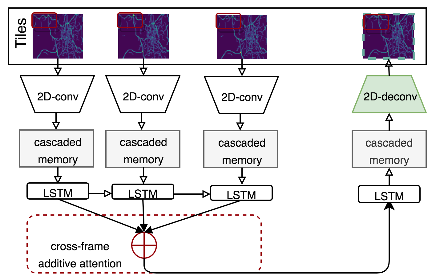
Figure 1: Encoder-decoder architecture

2.2 Tiled-based sampling and cross-frame attention

To deal with the high-resolution nature of the traffic frames, a common efficient approach is to split the frames into tiles, especially when the underlying map/ graph topology has grid-based sub-graph representations. Also, it is known from related work on taxi demand and traffic prediction, that simply applying CNN over the entire city as a sole image may not achieve the best performance (Yao et al. (2019)).

Also, motivated by mini-batch SGD in graph-based approaches (Chiang et al. (2019)), where each update is only based on a fixed-sized mini-batch gradient, it can reduce the memory requirement and conduct many updates per epoch, leading to a faster convergence.

Thus, our intuition for the attention layer is the weight distribution cross-frame is dependent on different tiles. For each tile $\mathcal{T}_{ij}$, the global context vector of the encoder is $\sum_{t}\alpha_{t}h_{t}$, where $\alpha_{t}$ is the normalized weight of a frame at time step $t$ (of the encoder), derived from the softmax of the alignment scores. Precisely, the score function is calculated as:

$$\text{(}score)(h_{t},d^{h}_{\bar{t}})=v_{\alpha}^{T}\text{tanh}(\mathbf{W}_{\alpha}[h_{t};d^{h}_{\bar{t}}])$$ (1)

where $v_{\alpha}$ and $\mathbf{W}_{\alpha}$ are learned weight matrices, $d^{h}_{\bar{t}}$ is the target state of the decoder, $h_{t}$ are the hidden states of the encoder. With this design, for a particular tile in a frame, there is a corresponding global attention map. Specifically, the representation of a tile can be freely learned from different temporal contexts.

3 Experiment

Datasets. The high-resolution traffic map videos for the challenge were derived from positions reported by a large fleet of probe vehicles over 12 months, and are based on over 100 billion probe points. Each video frame summarizes GPS trajectories (of 3 channels, encode speed, volume, and direction of traffic) mapped to spatio-temporal cells, sampled every 5 minutes and of size $495\times 436$. For the evaluation, we need to predict the next 3 frames over 5 predicting points over 72 days over 3 cities.

Implementation Details. We use 2D-conv LSTM as our base layer, and the number of memory-cascade layers are in the range of $[2,3,4]$, the number of hidden units in range of $[16,32,64]$. We split the frames into 48 tiles of size $62\times 73$, thus the logical batch-size is 48. All experiments are conducted over Nvidia Tesla v100 16/32GB gpus. We use the adjusted teacher forcing procedure for training. The code is open-sourced at: https://github.com/tumeteor/neurips2019challenge.

Results. We consider several baselines for the evaluation. As it also reflects in the leaderboard, the average model is a very strong competitor for this task. We report the results of our adjusted decay-based average, together with video prediction baselines (Tran et al. (2015); Wang et al. (2019b)). Our model trained with no tile-based sampling achieves quite good results, but it required the Tesla V with 32GB VRAM and took much longer time for convergence. The details are demonstrated in Table 3. We also witnessed that the tiling procedure does not perform well for all cities, in particular, the performance decreases slightly for the city of Istanbul. It is expected as for fixed-size tiling in images (as contrary to graph-based tiling) we might loose the local neighborhood information to a certain extent. A smoothing method is being looked into for future work.

Model	pixel-wise MSE
seq2seq	0.03211
3D-CNN (Tran et al. (2015))	0.01553
decay average	0.01014
cascaded memory (Wang et al. (2019b))	0.00977
ours-no-tiling	0.00957
ours	0.00952

4 Conclusion

We have presented an end-to-end recurrent neural network for spatiotemporal predictive learning for traffic video prediction. Our model achieves good performance and outperforms state-of-the-art models for video prediction on real-world high-resolution traffic datasets of three different cities.

Acknowledgments

We would like to thank Tuan Tran, Bosch CC for his valuable feedback, Peter Popov and Johannes Scheibe for their constant supports.

Appendix A Empirical implications

We illustrate the predictions from our model and the decay average in Figure 2. The visualizations show that the base map is encoded pretty well in our predictions (and the average), but the image does not look so realistic (compared to the last frames). We use the pix-2-pix L2 loss solely during training, but combining it with a GAN loss with adversarial training can probably be helpful in this case.

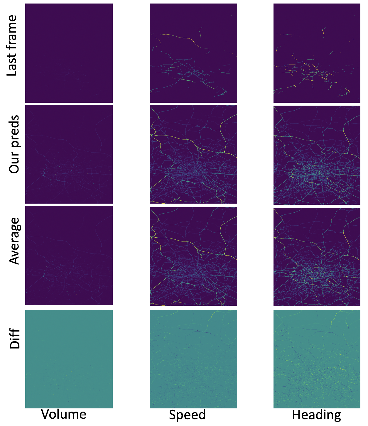
Figure 2: Prediction examples for every channel. Diff denotes the difference between ours and the 12 frames average.

References

- Chiang et al. [2019] W.-L. Chiang, X. Liu, S. Si, Y. Li, S. Bengio, and C.-J. Hsieh. Cluster-gcn: An efficient algorithm for training deep and large graph convolutional networks. arXiv preprint arXiv:1905.07953, 2019.
- Deng et al. [2016] D. Deng, C. Shahabi, U. Demiryurek, L. Zhu, R. Yu, and Y. Liu. Latent space model for road networks to predict time-varying traffic. In Proceedings of the 22nd ACM SIGKDD International Conference on Knowledge Discovery and Data Mining, pages 1525–1534. ACM, 2016.
- Fang et al. [2019] S. Fang, Q. Zhang, G. Meng, S. Xiang, and C. Pan. Gstnet: Global spatial-temporal network for traffic flow prediction. In Proceedings of the Twenty-Eighth International Joint Conference on Artificial Intelligence, IJCAI 2019, Macao, China, August 10-16, 2019, pages 2286–2293, 2019.
- Shin and Yoon [2019] Y. Y. Shin and Y. Yoon. Incorporating dynamicity of transportation network with multi-weight traffic graph convolution for traffic forecasting. arXiv preprint arXiv:1909.07105, 2019.
- Tong et al. [2017] Y. Tong, Y. Chen, Z. Zhou, L. Chen, J. Wang, Q. Yang, J. Ye, and W. Lv. The simpler the better: a unified approach to predicting original taxi demands based on large-scale online platforms. In Proceedings of the 23rd ACM SIGKDD international conference on knowledge discovery and data mining, pages 1653–1662. ACM, 2017.
- Tran et al. [2015] D. Tran, L. Bourdev, R. Fergus, L. Torresani, and M. Paluri. Learning spatiotemporal features with 3d convolutional networks. In Proceedings of the IEEE international conference on computer vision, pages 4489–4497, 2015.
- Wang et al. [2019a] Y. Wang, L. Jiang, M.-h. Yang, J. Li, M. Long, and F.-F. Li. Eidetic 3d lstm: A model for video prediction and beyond. 2019a.
- Wang et al. [2019b] Y. Wang, J. Zhang, H. Zhu, M. Long, J. Wang, and P. S. Yu. Memory in memory: A predictive neural network for learning higher-order non-stationarity from spatiotemporal dynamics. In IEEE Conference on Computer Vision and Pattern Recognition, CVPR2019, Long Beach, CA, USA, June 16-20, 2019, pages 9154–9162, 2019b.
- Xingjian et al. [2015] S. Xingjian, Z. Chen, H. Wang, D.-Y. Yeung, W.-K. Wong, and W.-c. Woo. Convolutional lstm network: A machine learning approach for precipitation nowcasting. In Advances in neural information processing systems, pages 802–810, 2015.
- Yao et al. [2019] H. Yao, X. Tang, H. Wei, G. Zheng, and Z. Li. Revisiting spatial-temporal similarity: A deep learning framework for traffic prediction. 2019.
- Zhang et al. [2018] L. Zhang, G. Zhu, L. Mei, P. Shen, S. A. A. Shah, and M. Bennamoun. Attention in convolutional lstm for gesture recognition. In Advances in Neural Information Processing Systems, pages 1953–1962, 2018.
- Zheng and Ni [2013] J. Zheng and L. M. Ni. Time-dependent trajectory regression on road networks via multi-task learning. In Twenty-Seventh AAAI Conference on Artificial Intelligence, 2013.