Pulse and continuously driven many-body quantum dynamics of
bosonic impurities in a Bose-Einstein condensate

Abstract

We unravel the periodically driven dynamics of two repulsively interacting bosonic impurities within a bosonic bath upon considering either the impact of a finite pulse or a continuous shaking of the impurities harmonic trap. Following a pulse driving of initially miscible components we reveal a variety of dynamical response regimes depending on the driving frequency. At resonant drivings the impurities decouple from their host while if exposed to a high frequency driving they remain trapped in the bosonic gas. For continuous shaking we showcase that in the resonantly driven regime the impurities oscillate back and forth within and outside the bosonic medium. In all cases, the bosonic bath is perturbed performing a collective dipole motion. Referring to an immiscible initial state we unveil that for moderate driving frequencies the impurities feature a dispersive behavior whilst for a high frequency driving they oscillate around the edges of the Thomas-Fermi background. Energy transfer processes from the impurities to their environment are encountered, especially for large driving frequencies. Additionally, coherence losses develop in the course of the evolution with the impurities predominantly moving as a pair.

I Introduction

Ultracold atoms constitute a unique testbed for monitoring the nonequilibrium quantum dynamics of strongly particle imbalanced multicomponent systems Will et al. (2011); Massignan et al. (2014); Palzer et al. (2009); Modugno et al. (2002); Burchianti et al. (2018). Recently, considerable attention has been devoted to the study of impurities in a many-body environment. The impurities are then dressed thereby forming quasiparticles Landau (1933); Fröhlich (1954) such as polarons Schmidt et al. (2018); Massignan et al. (2014). Consequently, this dressing mechanism affects fundamental properties of the impurities e.g. their effective mass Khandekar et al. (1988), mobility Feynman et al. (1962); Kadanoff (1963), induced interactions Massignan et al. (2014) and even allows them to form bound states known as bipolarons Casteels et al. (2013); Camacho-Guardian et al. (2018); Schmidt et al. (2018). The exquisite tunability of the ultracold environment, e.g. the manipulation of the interaction between the impurities and their host using Feshbach resonances Chin et al. (2010); Köhler et al. (2006), enabled the experimental realization of both Bose Jørgensen et al. (2016); Hu et al. (2016); Catani et al. (2009); Fukuhara et al. (2013) and Fermi polarons Scazza et al. (2017); Koschorreck et al. (2012); Kohstall et al. (2012) and the consecutive probing of their characteristics. These include, for instance, the quasiparticle excitation spectrum via radiofrequency spectroscopy Koschorreck et al. (2012); Kohstall et al. (2012); Cetina et al. (2015, 2016), the impurities trajectory employing in-situ imaging Catani et al. (2009); Fukuhara et al. (2013) and the crucial involvement of higher-order correlations Koepsell et al. (2019) for the adequate description of the polaronic states. Simultaneously, a vast amount of theoretical efforts have been mainly devoted to unravel the stationary properties of polaronic states Grusdt and Demler (2015) which range from the the Fröhlich model Bruderer et al. (2007); Casteels et al. (2012); Kain and Ling (2016); Casteels et al. (2013) to advanced beyond mean-field frameworks Volosniev and Hammer (2017); Dehkharghani et al. (2018); Mistakidis et al. (2019a); Jørgensen et al. (2016); Ardila and Pohl (2018); Ardila and Giorgini (2015); Ardila et al. (2019); Grusdt et al. (2018, 2017a); Grusdt and Demler (2015); Tempere et al. (2009); Panochko and Pastukhov (2019) that include interparticle correlations.

Having established an adequate understanding of the stationary properties of polarons, a natural next step which has been very recently put forward is to investigate their nonequilibrium dynamics Mistakidis et al. (2019b, c) revealing peculiar correlation effects Volosniev et al. (2015); Mistakidis et al. (2019c, d, b); Grusdt et al. (2018); Shchadilova et al. (2016); Kamar et al. (2019); Boyanovsky et al. (2019). Indeed, the crucial involvement of interparticle correlations can lead to non-linear structure formation Grusdt et al. (2017b); Mistakidis et al. (2019d), alterations of the breathing frequency Guebli and Boudjemâa (2019), the manifestation of orthogonality catastrophe phenomena Mistakidis et al. (2019c); Knap et al. (2012); Anderson (1967), dissipative motion of impurities in the many-body medium Mistakidis et al. (2019e) and also their relaxation dynamics Boyanovsky et al. (2019); Lausch et al. (2018). Other applications address impurity transport in optical lattices Cai et al. (2010); Johnson et al. (2011); Siegl et al. (2018); Theel et al. (2019), their collisional dynamics when penetrating with a finite velocity a gas of Tonks-Girardeau bosons Burovski et al. (2014); Lychkovskiy et al. (2018); Meinert et al. (2017); Knap et al. (2014); Gamayun et al. (2018), the effective control of quantum coherence Li and Kuang (2019) and investigations of three-body Effimov physics Yoshida et al. (2018); Blume (2019). However despite the above-mentioned first investigations, the impurities dynamics is still largely unexplored, especially in the case of more than a single impurity, while its further theoretical understanding is highly desirable and of growing interest with the aim to exploit this knowledge in the future for specific physical applications.

A promising driving protocol to study the emergent nonequilibrium dynamics of impurities corresponds to a periodic driving Goldman and Dalibard (2014); Goldman et al. (2015); Morsch and Oberthaler (2006) of their external potential. Here, the dependence of the impurities dynamical response on the driving frequency is of immediate interest in order to realize in which regimes Mistakidis et al. (2015); Mistakidis and Schmelcher (2017); Goldman and Dalibard (2014); Goldman et al. (2015) the impurities are dynamically trapped in their host or they can escape. Moreover the initial state of the system characterized as miscible when the impurities and the bath are spatially overlapping or immiscible in the opposite case is expected to crucially affect the dynamics. Another interesting prospect is to reveal induced impurity-impurity interactions Dehkharghani et al. (2018); Mistakidis et al. (2019f) mediated by the environment despite the existence of direct $\displaystyle s$-wave impurity-impurity repulsions. Furthermore, dynamical phase separation Mistakidis et al. (2018a); Erdmann et al. (2019); Ao and Chui (1998) and associated energy exchange Nielsen et al. (2019); Lampo et al. (2017) processes are worth studying. To track the driven nonequilibrium dynamics of the impurities capturing all relevant interparticle correlations we utilize the Multi-Layer Multi-Configuration Time-Dependent Hatree Method for atomic mixtures (ML-MCTDHX) Cao et al. (2017, 2013); Krönke et al. (2013). The latter is a non-perturbative variational approach especially designed to treat the correlated quantum dynamics of atomic mixtures exposed to time-dependent modulations. In particular, we consider two repulsively interacting bosonic impurities embedded in a Bose-Einstein condensate (BEC) and both being trapped in an external one-dimensional harmonic oscillator. To trigger the dynamics we apply a shaking of the harmonic potential of the impurities. This shaking is either performed for two driving periods and subsequently the system is left to evolve freely (pulse) or it is maintained throughout the evolution (continuous driving). The BEC is not impacted by the external driving. We focus on the case where the impurities and the bosonic gas are initially spatially overlapping (miscible components) while the case of an initially immiscible state is discussed briefly.

Focusing on the case of a pulse and initially miscible components we unveil a variety of dynamical response regimes of the impurities depending on the driving frequency. At small driving frequencies the impurities closely follow the motion of their trap Goldman and Dalibard (2014); Goldman et al. (2015) and after the pulse they remain trapped while oscillating inside the bosonic bath. Exposed to a resonant pulse Goldman and Dalibard (2014); Mistakidis et al. (2015); Mistakidis and Schmelcher (2017), namely the frequency of the finite pulse is similar to the one of the harmonic trap, the impurities perform a complex motion escaping and re-entering into their host and finally decoupling from the latter. Entering the strongly driven regime, the impurities remain trapped in the bosonic gas and show a dispersive behavior for long evolution times. Considering an immiscible initial state we observe that for moderate driving frequencies the impurities feature a dispersive behavior within the bosonic gas and when subjected to a highly intense driving they oscillate around the edges of the Thomas-Fermi background and the intercomponent spatial separation remains intact.

For a continuous shaking of the impurities trap and miscible components we showcase that an overall similar phenomenology to the non-continuously driven case occurs for very low and high driving frequencies. Interestingly, we observe that in the resonantly driven regime the impurities exhibit an irregular oscillatory motion, moving within and escaping from the BEC background, while featuring collisions with the latter. As a result of the impurities motion the bosonic gas is perturbed performing a collective dipole motion independently of the driving frequency and the protocol, a behavior that becomes more pronounced for high frequency drivings where the impurities predominantly reside within the bath.

Moreover, we reveal that when the impurities reside within the bosonic gas they dissipate energy into the latter Mistakidis et al. (2019a, e); Nielsen et al. (2019); Lampo et al. (2017), a process which is more prominent for large driving frequencies where the degree of inter- and intraspecies correlations Mistakidis et al. (2019d, e) is found to be enhanced. The development of coherence losses is unveiled by monitoring the time-evolution of the one-body coherence function Li and Kuang (2019), while the impurities two-body reduced density matrix shows that they travel predominantly as a pair Theel et al. (2019); Mistakidis et al. (2019d); Dehkharghani et al. (2018); Mistakidis et al. (2019g, f).

This work is structured as follows. Section II presents our setup and driving protocol as well as the many-body wavefunction ansatz and the observables which are utilized for the characterization of the periodically driven dynamics. In Section III we discuss the emergent periodically driven dynamics of miscible components induced by a pulse acting on the harmonic oscillator potential of the impurities. The driven dynamics of initially immiscible components is showcased in Sec. IV. Section V presents the periodically driven time-evolution of two miscible components corresponding to a continuous shaking. We summarize our results and provide an outlook in Section VI. In Appendix A we show that the dynamical response of the mixture is not significantly affected when considering two heavy impurities. Appendix B elaborates on the ingredients of the numerical simulations and delineates their convergence. Finally, Appendix C showcases the dynamics of two bosons in a shaken harmonic trap.

II Theoretical Framework

II.1 Hamiltonian and driving protocol

We consider a highly particle imbalanced bosonic mixture consisting of $\displaystyle N_{I}=2$ and $\displaystyle N_{B}=100$ atoms such that $\displaystyle N_{B}>>N_{I}$. Both species possess the same mass, i.e. $\displaystyle M_{I}=M_{B}=M$, and are confined in an one dimensional harmonic oscillator potential of frequency $\displaystyle\omega_{I}=\omega_{B}\equiv\omega=0.3$. Such a mass balanced mixture can be experimentally realized e.g. by a binary BEC of ⁸⁷Rb atoms prepared in the hyperfine states $\displaystyle\Ket{F=1,m_{F}=-1}$ and $\displaystyle\Ket{F=2,m_{F}=1}$ Egorov et al. (2013). The mixture is initialized in its ground state configuration (see also below) and in order to trigger the out-of-equilibrium dynamics the harmonic oscillator potential of the impurities is periodically shaken while the potential of the bosonic gas remains unperturbed. The corresponding many-body Hamiltonian reads

$$\begin{split}&H=\sum_{\sigma=B,I}\sum_{i=1}^{N_{\sigma}}-\frac{\hbar^{2}}{2M}\bigg{(}\frac{\partial}{\partial x_{i}^{\sigma}}\bigg{)}^{2}+\sum_{i=1}^{N_{B}}\frac{1}{2}M\omega(x_{i}^{B})^{2}\\ &+\sum_{i=1}^{N_{I}}V_{sh}^{I}(x^{I}_{i},t)+g_{BB}\sum_{i\geq j}\delta(x^{B}_{i}-x^{B}_{j})\\ &+g_{II}\sum_{i\geq j}\delta(x^{I}_{i}-x^{I}_{j})+g_{BI}\sum_{i=1}^{N_{B}}\sum_{j=1}^{N_{I}}\delta(x^{B}_{i}-x^{I}_{j}).\end{split}$$ (1)

Here, the periodically driven harmonic oscillator potential of the impurities takes the form

$$V_{sh}^{I}(x^{I},t)=\frac{1}{2}M\omega^{2}\big{(}x^{I}-\mathcal{A}\sin(\omega_{D}t)\big{)}^{2},$$ (2)

with $\displaystyle\mathcal{A}$ and $\displaystyle\omega_{D}$ being the amplitude and the frequency of the driving respectively. Experimentally, this periodically driven scheme can be accomplished e.g. via acousto-optical modulators Parker et al. (2013). Moreover we operate in the ultracold regime and hence $\displaystyle s$-wave scattering constitutes the dominant interaction process. Consequently, both the intra- and the interspecies interactions are modeled by a contact potential with effective coupling constants $\displaystyle g_{BB}$, $\displaystyle g_{II}$ and $\displaystyle g_{BI}$. The effective one-dimensional coupling strength Olshanii (1998) acquires the form $\displaystyle{g_{\sigma\sigma^{\prime}}}=\frac{{2{\hbar^{2}}{a^{s}_{\sigma\sigma^{\prime}}}}}{{\mu a_{\bot}^{2}}}{\left({1-{\left|{\zeta(1/2)}\right|{a^{s}_{\sigma\sigma^{\prime}}}}/{{\sqrt{2}{a_{\bot}}}}}\right)^{-1}}$, with $\displaystyle\sigma,\sigma^{\prime}=B,I$, $\displaystyle\mu=\frac{M}{2}$ being the reduced mass and $\displaystyle\zeta$ is the Riemann zeta function. The transverse length scale is set by $\displaystyle a_{\perp}=\sqrt{\hbar/M\omega_{\perp}}$, where $\displaystyle\omega_{\perp}$ is the frequency of the transverse confinement. Additionally, $\displaystyle{a^{s}_{\sigma\sigma^{\prime}}}$ is the three-dimensional $\displaystyle s$-wave intra ($\displaystyle\sigma=\sigma^{\prime}$) or interspecies ($\displaystyle\sigma\neq\sigma^{\prime}$) scattering length. As a result $\displaystyle g_{\sigma\sigma^{\prime}}$ can be tuned experimentally via $\displaystyle{a^{s}_{\sigma\sigma^{\prime}}}$ through Feshbach resonances Köhler et al. (2006); Chin et al. (2010) or by manipulating $\displaystyle{{\omega_{\bot}}}$ with the aid of confinement-induced resonances Olshanii (1998).

For convenience, below, the many-body Hamiltonian of Eq. (1) is casted in units of $\displaystyle\hbar\omega_{\perp}$. Consequently, the length, time and the interaction strength are rescaled in units of $\displaystyle\sqrt{\hbar/M\omega_{\perp}}$, $\displaystyle\omega^{-1}_{\perp}$, and $\displaystyle\sqrt{\hbar^{3}\omega_{\perp}/M}$, respectively. Also, the frequency $\displaystyle\omega$ of the harmonic oscillator and the driving frequency $\displaystyle\omega_{D}$ are expressed in terms of $\displaystyle\omega_{\perp}$. To restrict the spatial extent of the system we employ hard-wall boundary conditions at $\displaystyle x_{\pm}=\pm 50$ which do not affect the dynamics since there is not any appreciable density population beyond $\displaystyle x_{\pm}=\pm 25$.

Our system consisting of $\displaystyle N_{I}=2$ impurities and $\displaystyle N_{B}=100$ atoms in the bosonic bath is initially prepared in its many-body ground state described by the Hamiltonian of Eq. (1) with $\displaystyle\omega=0.3$, $\displaystyle\omega_{D}=0$ and $\displaystyle\mathcal{A}=0$. Throughout this work, the intraspecies interaction strengths are kept fixed to the values $\displaystyle g_{II}=0.4$ and $\displaystyle g_{BB}=0.5$, unless it is stated otherwise. Having obtained the many-body ground state of the system with the above-mentioned parameters, we induce its nonequilibrium dynamics by considering a periodic driving of the impurities harmonic oscillator potential [Eq. (2)] while the bosonic bath remains undriven. In particular, we employ two different driving protocols. Namely in the first one, which we shall term below the pulse driving, the potential of the impurities is periodically driven for only two driving periods, i.e. until $\displaystyle t_{f}=4\pi/\omega_{D}$, and afterwards the system is let to evolve freely. However, in the second scenario the impurities are continuously driven throughout the dynamics.

II.2 Many-body wavefunction ansatz

To unravel the periodically driven dynamics of the binary bosonic mixture we employ the variational ML-MCTDHX Cao et al. (2017, 2013); Krönke et al. (2013) method. It is based on expanding the total many-body wavefunction of the system with respect to a time-dependent and variationally optimized basis set. This allows us to take into account both the intra- and the interspecies correlations of the binary system using a numerically feasible size of the basis set. The total many-body wavefunction can be expressed in the form of a truncated Schmidt decomposition Horodecki et al. (2009) of rank $\displaystyle D$ as follows

$$\Psi_{MB}(\vec{x}^{B},\vec{x}^{I};t)=\sum_{k=1}^{D}\sqrt{\lambda_{k}(t)}\Psi^{B}_{k}(\vec{x}^{B};t)\Psi^{I}_{k}(\vec{x}^{I};t).$$ (3)

The time-dependent basis states $\displaystyle\Psi^{\sigma}_{k}(\vec{x}^{\sigma};t)$ form an orthonormal $\displaystyle N_{\sigma}$-body wavefunction set in a subspace of the $\displaystyle\sigma$-species Hilbert space $\displaystyle\mathcal{H}^{\sigma}$ and are known as the species functions of the $\displaystyle\sigma$-species. Moreover, the Schmidt coefficients $\displaystyle\lambda_{k}(t)$ in decreasing order are referred to as the natural species populations of the $\displaystyle k$-th species function. These coefficients signify the presence of entanglement of the system. In particular, if there is only one non-vanishing Schmidt coefficient, then the total many-body state of Eq. (3) is a direct product of the two species states and the system is non-entangled. In contrast, when at least two $\displaystyle\lambda_{k}(t)$ possess a non-zero value, the system is termed entangled or interspecies correlated Roncaglia et al. (2014).

Next in order to incorporate intraspecies correlations into our many-body ansatz we expand each of the species functions $\displaystyle\Psi^{\sigma}_{k}(\vec{x}^{\sigma};t)$ with respect to permanents of $\displaystyle d_{\sigma}$ distinct time-dependent single-particle functions (SPFs) $\displaystyle\varphi_{1}^{\sigma},\dots,\varphi_{d_{\sigma}}^{\sigma}$. Then, $\displaystyle\Psi^{\sigma}_{k}(\vec{x}^{\sigma};t)$ reads

$$\begin{split}&\Psi_{k}^{\sigma}(\vec{x}^{\sigma};t)=\sum_{\begin{subarray}{c}l_{1},\dots,l_{d_{\sigma}}\\ \sum l_{i}=N\end{subarray}}C_{k,(l_{1},\dots,l_{d_{\sigma}})}(t)\\ &\times\sum_{i=1}^{N_{\sigma}!}\mathcal{P}_{i}\left[\prod_{j=1}^{l_{1}}\varphi_{1}^{\sigma}(x_{j};t)\cdots\prod_{j=1}^{l_{d_{\sigma}}}\varphi_{d_{\sigma}}^{\sigma}(x_{K(d_{\sigma})+j};t)\right].\end{split}$$ (4)

Here, $\displaystyle\mathcal{P}$ is the permutation operator which exchanges the particle positions $\displaystyle x_{\nu}^{\sigma}$, $\displaystyle\nu=1,\dots,N_{\sigma}$ within the SPFs. Also, $\displaystyle K(r)\equiv\sum_{\nu=1}^{r-1}l_{\nu}$, with $\displaystyle l_{\nu}$ being the occupation of the $\displaystyle\nu$th SPF and $\displaystyle r\in\{1,2,\dots,d_{\sigma}\}$ and $\displaystyle C_{k,(l_{1},\dots,l_{d_{\sigma}})}(t)$ are the time-dependent expansion coefficients. The eigenfunctions of the $\displaystyle\sigma$-species one-body reduced density matrix $\displaystyle\rho_{\sigma}^{(1)}(x,x^{\prime};t)=\langle\Psi_{MB}(t)|\hat{\Psi}^{\sigma\dagger}(x)\hat{\Psi}^{\sigma}(x^{\prime})|\Psi_{MB}(t)\rangle$ are termed natural orbitals $\displaystyle\phi^{\sigma}_{i}(x;t)$. Note that $\displaystyle\hat{\Psi}^{\sigma}(x)$ is the $\displaystyle\sigma$-species bosonic field operator. The natural orbitals are related with the SPFs by employing a unitary transformation that diagonalizes $\displaystyle\rho_{\sigma}^{(1)}(x,x^{\prime};t)$ when it is expressed in the basis of SPFs, see also Cao et al. (2017, 2013); Krönke et al. (2013) for details. The eigenvalues of $\displaystyle\rho_{\sigma}^{(1)}(x,x^{\prime};t)$ are the so-called natural populations $\displaystyle n^{\sigma}_{i}(t)$ and provide a measure for the occurrence of the $\displaystyle\sigma$-species intraspecies correlations. Indeed, the $\displaystyle\sigma$-species subsystem is intraspecies correlated if more than one eigenvalue is macroscopically occupied, otherwise it is termed fully coherent.

Having specified the many-body wavefunction ansatz introduced in Eqs. (3) and (4) one determines the corresponding ML-MCTDHX equations of motion Cao et al. (2017); Köhler et al. (2019) of the constituents $\displaystyle\lambda_{k}(t)$, $\displaystyle C_{k,(l_{1},\dots,l_{d_{\sigma}})}(t)$ and $\displaystyle\phi^{\sigma}_{j}(x^{\sigma};t)$. Indeed, by utilizing e.g. the Dirac-Frenkel variational principle Frenkel (1934); Dirac (1930) one arrives at a set of $\displaystyle D^{2}$ linear differential equations for the coefficients $\displaystyle\lambda_{k}(t)$, which are coupled to $\displaystyle D\big{[}(N_{B}+d_{B}-1)!/N_{B}!(d_{B}-1)!+(N_{I}+d_{I}-1)!/N_{I}!(d_{I}-1)!\big{]}$ non-linear integrodifferential equations for $\displaystyle C_{k,(l_{1},\dots,l_{d_{\sigma}})}(t)$ and $\displaystyle d_{I}+d_{B}$ nonlinear integrodifferential equations for the SPFs. Note that for all many-body simulations, to be presented below, we use $\displaystyle D=10$ species functions and $\displaystyle d_{B}=3$, $\displaystyle d_{I}=6$ single-particle functions. In this way, numerical convergence is achieved, see Appendix B for a more elaborated discussion. For explicit derivations and further details we refer the reader to Refs. Cao et al. (2017, 2013); Krönke et al. (2013).

II.3 Observables of interest

We next introduce the main observables which will be employed for the interpretation of the periodically driven dynamics of the bosonic mixture. To estimate the degree of spatial one-body coherence in the course of the evolution, we invoke the normalized spatial first order correlation function Mistakidis et al. (2018a); Naraschewski and Glauber (1999); Sakmann et al. (2008)

$$\displaystyle g^{(1)}_{\sigma}(x,x^{\prime};t)=\frac{\rho_{\sigma}^{(1)}(x,x^{\prime};t)}{\sqrt{\rho_{\sigma}^{(1)}(x;t)\rho_{\sigma}^{(1)}(x^{\prime};t)}}.$$ (5)

Here, the $\displaystyle\sigma$-species one-body reduced density matrix is defined as $\displaystyle\rho_{\sigma}^{(1)}(x,x^{\prime};t)=\langle\Psi_{MB}(t)|\hat{\Psi}^{\sigma\dagger}(x)\hat{\Psi}^{\sigma}(x^{\prime})|\Psi_{MB}(t)\rangle$ whose diagonal corresponds to the one-body density $\displaystyle\rho_{\sigma}^{(1)}(x;t)\equiv\rho_{\sigma}^{(1)}(x,x^{\prime}=x;t)$ which is accessible in cold-atom experiments via in-situ imaging Catani et al. (2009); Fukuhara et al. (2013). Also, $\displaystyle\hat{\Psi}^{\sigma\dagger}(x)$ [$\displaystyle\hat{\Psi}^{\sigma}(x)$] is the bosonic field operator that creates [annihilates] a $\displaystyle\sigma$-species boson at position $\displaystyle x$. $\displaystyle|g^{(1)}_{\sigma}(x,x^{\prime};t)|$ takes values in the interval $\displaystyle[0,1]$ and indicates the proximity of the many-body state to a mean-field product state for a specific set of spatial coordinates $\displaystyle x$, $\displaystyle x^{\prime}$. Moreover, two distinct spatial regions $\displaystyle\mathcal{D}$, $\displaystyle\mathcal{D^{\prime}}$, i.e. $\displaystyle\mathcal{D}\cap\mathcal{D^{\prime}}=\varnothing$, are termed perfectly incoherent or fully coherent if $\displaystyle|g^{(1)}_{\sigma}(x,x^{\prime};t)|=0$ and $\displaystyle|g^{(1)}_{\sigma}(x,x^{\prime};t)|=1$ respectively with $\displaystyle x\in\mathcal{D}$ and $\displaystyle x^{\prime}\in\mathcal{D^{\prime}}$. Additionally in the case of partial incoherence, namely $\displaystyle 0<|g^{(1)}_{\sigma}(x,x^{\prime};t)|<1$, we can infer the development of one-body intraspecies correlations while full coherence $\displaystyle|g^{(1)}_{\sigma}(x,x^{\prime};t)|=1$ for every $\displaystyle x$, $\displaystyle x^{\prime}$ designates their absence.

To quantify the degree of impurity-BEC interspecies correlations or entanglement during the time-evolution we exploit the so-called von-Neumann entropy Horodecki et al. (2009); Erdmann et al. (2019); Catani et al. (2009)

$$\displaystyle S_{VN}(t)=-\sum\limits_{k=1}^{D}\lambda_{k}(t)\ln[\lambda_{k}(t)].$$ (6)

where $\displaystyle\lambda_{k}(t)$ denote the Schmidt coefficients [Eq. (3)]. The latter are the eigenvalues of the species reduced density matrix e.g. $\displaystyle\rho^{(N_{B})}(\vec{x}^{B},\vec{x}^{\prime B};t)=\int dx^{I}\Psi^{*}_{MB}(\vec{x}^{B},x^{I};t)\Psi_{MB}(\vec{x}^{\prime B},x^{I};t)$ where $\displaystyle\vec{x}^{B}=(x^{B}_{1},\cdots,x^{B}_{N_{B-1}})$. The binary system is species entangled or interspecies correlated if more than a single eigenvalue of $\displaystyle\rho^{N_{B}}$ possess a non-zero value, otherwise it is non-entangled [see also Eq. 3)]. For instance, within the mean-field approximation $\displaystyle\lambda_{1}(t)=1$ and $\displaystyle\lambda_{k}(t)=0$, $\displaystyle k=2,3,\dots,D$ and therefore $\displaystyle S_{VN}(t)=0$, while for a many-body state where $\displaystyle\lambda_{k>1}\neq 0$ it holds that $\displaystyle S_{VN}(t)\neq 0$.

The eigenfunctions of the $\displaystyle\sigma$-species one-body reduced density matrix $\displaystyle\rho^{(1)}_{\sigma}(x,x^{\prime};t)$ are the so-called $\displaystyle\sigma$-species natural orbitals, $\displaystyle\phi^{\sigma}_{i}(x;t)$, and natural populations $\displaystyle\eta^{\sigma}_{i}(t)\in[0,1]$ respectively. Each bosonic subsystem is said to be fragmented or intraspecies correlated if more than one natural population possesses a macroscopic occupation, otherwise the corresponding subsystem is fully coherent. Indeed, if the natural populations obey $\displaystyle\eta^{\sigma}_{1}(t)=1$, $\displaystyle\eta^{\sigma}_{i\neq 0}(t)=0$ [see also Eq. (3) and Eq. (4)] then the first natural orbital $\displaystyle\phi^{\sigma}_{1}$ becomes the Gross-Pitaevskii wavefunction $\displaystyle\phi^{\sigma}(x^{\sigma};t)$ Kevrekidis et al. (2007). Accordingly, we invoke as a measure of the $\displaystyle\sigma$-species intraspecies correlations the deviation

$$\mathcal{F}_{\sigma}(t)=1-\eta^{\sigma}_{1}(t).$$ (7)

It provides a theoretical tool for the identification of the occupation of the $\displaystyle d_{\sigma}>1$ least occupied bosonic natural orbitals, and therefore of the deviation of the many-body from a product state when $\displaystyle\mathcal{F}_{\sigma}(t)>0$ Katsimiga et al. (2017a, 2018, b).

To monitor the position of the center-of-mass of the $\displaystyle\sigma$-species during the nonequilibrium dynamics we resort to its spatially averaged mean position

$$\braket{X_{\sigma}(t)}=\braket{\Psi_{MB}(t)}{\hat{x}^{\sigma}}{\Psi_{MB}(t)},$$ (8)

In this expression, $\displaystyle\hat{x}^{\sigma}=\int_{\mathcal{R}}dxx^{\sigma}\hat{\Psi}^{\sigma\dagger}(x)\hat{\Psi}^{\sigma}(x)$ represents a one-body operator and $\displaystyle\mathcal{R}$ is the spatial extension of the $\displaystyle\sigma$-species one-body density. This quantity, $\displaystyle\braket{X_{\sigma}(t)}$, can be assessed experimentally by relying on spin-resolved single-shot absorption images Catani et al. (2009); Fukuhara et al. (2013). More precisely, each individual image gives an estimate of the $\displaystyle\sigma$-species position while $\displaystyle\braket{X_{\sigma}(t)}$ can be retrieved by averaging over several such images Katsimiga et al. (2017b); Mistakidis et al. (2019e, 2018b).

III Driving with a two period pulse

In this section we discuss the nonequilibrium dynamics of the bosonic mixture induced by a two period pulse driving of the harmonic oscillator of the impurity atoms. The system consisting of $\displaystyle N_{B}=100$ bosons and $\displaystyle N_{I}=2$ impurities, both being confined in the same harmonic potential of frequency $\displaystyle\omega=0.3$, is initially prepared in its many-body ground state with $\displaystyle g_{BB}=0.5$, $\displaystyle g_{II}=0.4$ and $\displaystyle g_{BI}=0.2$. Note that this choice of the interaction parameters ensures that the system initially ($\displaystyle t=0$) resides within the miscible phase since $\displaystyle g_{BI}<\sqrt{g_{BB}g_{II}}$ Ao and Chui (1998); Timmermans (1998). To trigger the dynamics the harmonic oscillator potential of the impurities is periodically shaken according to Eq. (2) for two driving periods i.e. up to a finite time $\displaystyle t_{f}=4\pi/\omega_{D}$ where $\displaystyle\omega_{D}$ is the driving frequency. Also here we consider an oscillation amplitude $\displaystyle\mathcal{A}=20\gg R_{TF}$ with $\displaystyle R_{TF}\approx 8.3$ denoting the Thomas-Fermi radius of the bosonic gas. Then for $\displaystyle t>t_{f}$ the system is left to evolve freely, namely without any external driving, while keeping fixed all other parameters for a specific $\displaystyle\omega_{D}$.

Moreover, we cover a wide range of driving frequencies lying in the interval $\displaystyle\omega_{D}\in[0.025,2]$. Let us note in passing that the overall phenomenology, to be presented below, does not significantly depend on the value of the driving amplitude $\displaystyle\mathcal{A}$. We have verified this by inspecting the dynamics also for $\displaystyle\mathcal{A}=10$ and $\displaystyle\mathcal{A}=5$ (not shown for brevity).

III.1 Single-particle density evolution

In order to inspect the periodically driven dynamics, we first invoke the time-evolution of the $\displaystyle\sigma$-species single-particle density, $\displaystyle\rho^{(1)}_{\sigma}(x;t)$ shown in Fig. 1 for specific driving frequencies covering the low to high frequency regimes. For low frequencies such as $\displaystyle\omega_{D}=0.075$, the impurities which are initially located at the trap center follow the motion of their external trapping potential moving towards the left edge of the bosonic gas [Fig. 1 ($\displaystyle b_{1}$)]. In this time interval $\displaystyle\rho^{(1)}_{I}(x;t)$ becomes more squeezed than $\displaystyle\rho^{(1)}_{I}(x;t=0)$ [compare the width of $\displaystyle\rho^{(1)}_{I}(x;t=5)$ and $\displaystyle\rho^{(1)}_{I}(x;t=0)$ in Fig. 1 ($\displaystyle b_{1}$)] due to the interaction of the finite velocity impurities with the BEC background. Then, at $\displaystyle t=9.2$ the impurities escape from their host reaching the position $\displaystyle x=27$ at $\displaystyle t=16$ [Fig. 1 ($\displaystyle b_{1}$)] which lies beyond the driving amplitude ($\displaystyle\mathcal{A}=20$) and consequently they are reflected back due to the presence of the trap. During this latter motion they scatter back for a short time interval when approaching the bosonic gas [see the white dashed rectangle in Fig. 1 ($\displaystyle b_{1}$)] and then reverse again their direction traveling towards the BEC which they penetrate at $\displaystyle t=40$. Note here that this weak amplitude back-scattering event is mainly caused by the driving of the harmonic trap. In particular, it stems from the difference between the instantaneous velocity of the impurities and the external driving at specific spatial regions. Moreover, this event is only slightly enhanced by the presence of the repulsive $\displaystyle g_{BI}$, see also Appendix C.

Afterwards, the impurities dive into the bosonic bath, they reach its right edge and subsequently escape performing a similar to the above-described back and forth motion caused by the driven harmonic oscillator until they are again injected into the bosonic medium [Fig. 1 ($\displaystyle b_{1}$)]. In this way the first oscillation of the external driving potential is completed. During the second oscillation period the same overall phenomenology described above occurs until $\displaystyle t_{f}=166.07$ where the driving is terminated, see the dashed vertical line in Fig. 1 ($\displaystyle b_{1}$). Subsequently, the impurities remain confined within the BEC exhibiting an oscillatory motion characterized by an amplitude of the order of the Thomas-Fermi radius of the bosonic gas and do not escape from the latter (see also the discussion in Sec. III.2). As a consequence of the impurities motion and their interaction with the BEC background $\displaystyle\rho^{(1)}_{B}(x;t)$ exhibits weak distortions from its original Thomas-Fermi profile Mistakidis et al. (2019e) manifested by a small amplitude collective dipole mode [Fig. 1 ($\displaystyle a_{1}$)] in the course of time.

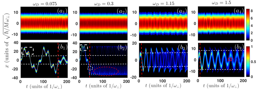
Figure 1: Time-evolution of the $\displaystyle\sigma$-species single-particle density $\displaystyle\rho^{(1)}_{\sigma}(x;t)$ of ($\displaystyle a_{1}$)-($\displaystyle a_{4}$) the bosonic bath ($\displaystyle\sigma=B$) and ($\displaystyle b_{1}$)-($\displaystyle b_{4}$) the two impurities ($\displaystyle\sigma=I$) for specific driving frequencies $\displaystyle\omega_{D}$ (see legends). The shaking of the external potential of the impurities is maintained up to $\displaystyle t_{f}=4\pi/\omega_{D}$ (see the dashed vertical line) and then the system is left to evolve. The bosonic mixture consists of $\displaystyle N_{B}=100$ atoms with $\displaystyle g_{BB}=0.5$ and $\displaystyle N_{I}=2$ interacting $\displaystyle g_{II}=0.4$ impurities and it is trapped in a harmonic oscillator of frequency $\displaystyle\omega=0.3$. The interspecies repulsion is $\displaystyle g_{BI}=0.2$ and the system is prepared in its ground state. The dashed horizontal and vertical lines in ($\displaystyle b_{1}$)-($\displaystyle b_{4}$) indicate the location of the Thomas-Fermi radius of the bosonic gas and the time-instant ($\displaystyle t=t_{f}$) of the termination of the shaking. The white dashed rectangles in ($\displaystyle b_{1}$), ($\displaystyle b_{2}$) mark the back-scattering events of the impurities. The dashed circle and ellipse in ($\displaystyle b_{2}$) mark the splitting of $\displaystyle\rho^{(1)}_{I}(x;t)$ and the portion of the impurities deposited at $\displaystyle x<0$ respectively for $\displaystyle t>t_{f}$, while the rectangle in ($\displaystyle b_{4}$) indicates the density notch of $\displaystyle\rho^{(1)}_{I}(x;t)$.

Increasing the driving frequency to $\displaystyle\omega_{D}=\omega=0.3$ (resonant driving) the impurities show a much more complex dynamical response [Fig. 1 ($\displaystyle b_{2}$)]. More precisely, at the initial stages of the dynamics they travel in the direction of the driving towards the left edge of the BEC and escape from the latter at $\displaystyle t=6$. Consequently they move until reaching $\displaystyle x=33.28$ where they are reflected back due to the driven harmonic trap and exhibit a back and forth motion experiencing two back-scattering events when approaching the boundary of the bosonic bath, see the white dashed rectangle in Fig. 1 ($\displaystyle b_{2}$). As time evolves the impurities are again injected into the bath at $\displaystyle t=24.8$ and interact with the latter.

Later on, they reach the right edge of the BEC at $\displaystyle t=38.1$ and escape moving outwards until they arrive at the position $\displaystyle x=33.3$ where they feel the external oscillator and are reflected backwards. During this backward motion the external driving stops at $\displaystyle t=41.87$ [dashed vertical line in Fig. 1 ($\displaystyle b_{2}$)] and when the impurities approach the right edge of the bosonic gas they interact with the latter and split into two fragments [see the dashed circle in Fig. 1 ($\displaystyle b_{2}$)] from which one transmits through the BEC ($\displaystyle x>-R_{TF}$) and the other one is reflected back ($\displaystyle x<R_{TF}$). The reflected part [see the dashed ellipse in Fig. 1 ($\displaystyle b_{2}$)] possesses the major population and it remains in the right region outside of the bath throughout the evolution showing a dispersive behavior. On the other hand the transmitted portion of $\displaystyle\rho^{(1)}_{I}(x,t)$ performs a large amplitude oscillatory motion penetrating and escaping $\displaystyle\rho^{(1)}_{B}(x,t)$ during the time-evolution. Therefore after the driving the major portion of the impurities is deposited outside the right edge of the bath and as a consequence the symmetry of the population of the impurities with respect to the trap center is broken for $\displaystyle\omega_{D}=\omega$. The bosonic bath remains essentially unperturbed during the dynamics since the impurities are most of the time out of their host, see Fig. 1 ($\displaystyle a_{2}$).

Next, we turn our attention to relatively fast drivings such that $\displaystyle\omega_{D}\gg\omega$ [Figs. 1 ($\displaystyle b_{3}$), ($\displaystyle b_{4}$)] where the time scale of the shaking $\displaystyle 1/\omega_{D}$ is much shorter than all the other relevant time scales of the system. Note that in this case it is exceedingly difficult for the impurities to adjust their motion to the external periodic variation of the position of the trap minimum and therefore the spatial extension of $\displaystyle\rho^{(1)}_{I}(x,t)$ is limited to a much smaller spatial region than the driving amplitude $\displaystyle\mathcal{A}$ Goldman and Dalibard (2014); Goldman et al. (2015); Mistakidis et al. (2015). To support our arguments we present exemplarily the time-evolution of $\displaystyle\rho^{(1)}_{I}(x,t)$ corresponding to frequencies $\displaystyle\omega_{D}=1.15$ [Fig. 1 ($\displaystyle b_{3}$)] and $\displaystyle\omega_{D}=1.5$ [Fig. 1 ($\displaystyle b_{4}$)]. Evidently, the oscillation amplitude of $\displaystyle\rho^{(1)}_{I}(x;t)$ in both cases is smaller than $\displaystyle\mathcal{A}$. For instance when $\displaystyle\omega_{D}=1.15$, $\displaystyle\rho^{(1)}_{I}(x;t)$ remains inside the bath within the time period of the shaking ($\displaystyle t<t_{f}=10.92$) while for $\displaystyle t>t_{f}$ it exhibits a periodic oscillation with an amplitude that exceeds the Thomas-Fermi radius of the BEC. Moreover, $\displaystyle\rho^{(1)}_{I}(x;t)$ has a localized shape for $\displaystyle t<44$ and later on it is gradually smeared out showing a relatively delocalized behavior for the time-intervals that the impurities lie within the bosonic gas, see Fig. 1 ($\displaystyle b_{3}$). This delocalized behavior $\displaystyle\rho^{(1)}_{I}(x;t)$ is caused by the interaction of the impurities with the atoms of the bath. However, when the impurities reside outside the edges of the BEC $\displaystyle\rho^{(1)}_{I}(x;t)$ forms localized spikes [Fig. 1 $\displaystyle(b_{3}$)]. The above-described dynamical response of the impurities, occurring for fast drivings, becomes more pronounced for even larger driving frequencies e.g. $\displaystyle\omega_{D}=1.5$ shown in Fig. 1 ($\displaystyle b_{4}$). Indeed, $\displaystyle\rho^{(1)}_{I}(x;t)$ remains localized while oscillating mostly within the bosonic cloud throughout the dynamics and a decay of its oscillation amplitude occurs as time evolves. Additionally, as a consequence of the impurity-BEC interaction a density notch builds upon $\displaystyle\rho^{(1)}_{I}(x;t)$ for $\displaystyle t>105$ [see the red square box in Fig. 1 $\displaystyle(b_{4})$] which essentially indicates the involvement of excited states in the dynamics of the impurities. For these fast drivings the impurities motion leave its traces on the bosonic bath manifested by the stripe patterns observed in $\displaystyle\rho^{(1)}_{B}(x;t)$, see Figs. 1 ($\displaystyle a_{3}$), ($\displaystyle a_{4}$). These stripe patterns reveal that the bosonic gas becomes excited due to its interaction with the impurities Mistakidis et al. (2019e, d) and are visualized as weak distortions from its original Thomas-Fermi profile. Most importantly, we can deduce that the excitations of the bosonic medium are much more prominent for fast driving frequencies compared to weak ones since in the former case the impurities mostly reside within the majority species cloud in the course of the evolution [Figs. 1 ($\displaystyle a_{3}$), ($\displaystyle a_{4}$)] while in the latter case they escape from the BEC background [Figs. 1 ($\displaystyle a_{1}$), ($\displaystyle a_{2}$)].

A remark regarding the dynamical dressing of the impurities from the excitations of the BEC background is appropriate at this point. Indeed, the above-described response of the impurities to their external driving suggests that their dynamical dressing and therefore the probability to form a quasiparticle, here the Bose polaron, is enhanced for high driving frequencies where they mainly reside within the bosonic bath. However, for resonant drivings ($\displaystyle\omega_{D}=\omega$) the impurities after the termination of the driving lie outside the BEC background [Fig. 1 ($\displaystyle b_{2}$)] and as a result we can ensure that no quasiparticle is formed Schmidt et al. (2018); Massignan et al. (2014); Cetina et al. (2016); Mistakidis et al. (2019b).

III.2 Time-evolution of the center-of-mass

To gain a better understanding of the dynamical response of each species due to the periodic driving of the impurities external potential, we subsequently inspect the position of the $\displaystyle\sigma$-species center-of-mass motion captured via $\displaystyle\langle X_{\sigma}(t)\rangle$ [Eq. (8)] for different $\displaystyle\omega_{D}$ [Figs. 2 ($\displaystyle a_{1}$)-($\displaystyle a_{4})$ and ($\displaystyle b_{1}$)-($\displaystyle b_{4}$)]. Below, we first analyze $\displaystyle\langle X_{I}(t)\rangle$ since the impurities undergo a much more involved dynamics than the bosonic gas as argued previously. Recall that the impurities are directly exposed to the external driving protocol whilst the bath is only indirectly affected by their motion.

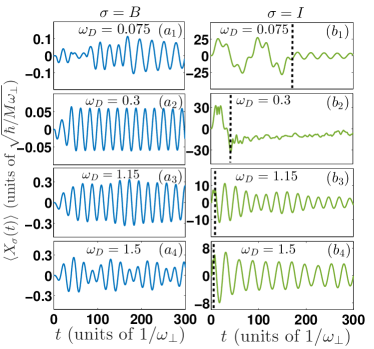
Figure 2: Temporal-evolution of the center-of-mass $\displaystyle\langle X_{\sigma}(t)\rangle$ of the impurities ($\displaystyle\sigma=I$) and the bath ($\displaystyle\sigma=B$) at selective driving frequencies ($\displaystyle a_{1}$), ($\displaystyle b_{1}$) $\displaystyle\omega_{D}=0.075$, ($\displaystyle a_{2}$), ($\displaystyle b_{2}$) $\displaystyle\omega_{D}=0.3$, ($\displaystyle a_{3}$), ($\displaystyle b_{3}$) $\displaystyle\omega_{D}=1.15$ and ($\displaystyle a_{4}$), ($\displaystyle b_{4}$) $\displaystyle\omega_{D}=1.5$. The dynamics is triggered by shaking the harmonic oscillator of the impurities for $\displaystyle t_{f}=4\pi/\omega_{D}$ (see the dashed vertical lines) and then the system is left to evolve unperturbed. Recall that the Thomas-Fermi radius of the bosonic gas is $\displaystyle R_{TF}\approx 8.3$. All other system parameters are the same as in Fig. 1.

Focusing on low driving frequencies i.e. $\displaystyle\omega_{D}=0.075\ll\omega$ we observe that the dynamics of $\displaystyle\langle X_{I}(t)\rangle$ closely resembles the evolution of $\displaystyle\rho^{(1)}_{I}(x;t)$, compare Figs. 1 ($\displaystyle b_{1}$) and Fig. 2 ($\displaystyle b_{1}$). This is a consequence of the mere fact that for such low driving frequencies the impurities can adequately adapt to the externally driven trapping potential and therefore $\displaystyle\rho^{(1)}_{I}(x,t)$ remains well localized at the instantaneous trap minimum. In particular, for $\displaystyle t<t_{f}$, $\displaystyle\langle X_{I}(t)\rangle$ shows an “irregular” oscillatory behavior with an amplitude larger than the actual driving amplitude $\displaystyle\mathcal{A}=20$ [Fig. 2 ($\displaystyle b_{1}$)]. However, when the driving is terminated at $\displaystyle t_{f}=166.47$ the oscillation amplitude of $\displaystyle\langle X_{I}(t)\rangle$ decreases drastically being much smaller than the Thomas-Fermi radius indicating that the impurities remain inside the BEC. Note also that in this latter time-interval the oscillation of $\displaystyle\langle X_{I}(t)\rangle$ possesses predominantly a single frequency. A similar “irregular” oscillatory pattern of $\displaystyle\langle X_{I}(t)\rangle$ takes place also for resonant drivings $\displaystyle\omega_{D}=0.3$ when $\displaystyle t<t_{f}=41.87$ but with a comparatively larger oscillation amplitude than $\displaystyle\omega_{D}=0.075$, see Fig. 2 ($\displaystyle b_{2}$). Subsequently for $\displaystyle t>t_{f}$ the center-of-mass oscillation amplitude of the impurities is greatly suppressed and in particular $\displaystyle\langle X_{I}(t)\rangle$ is restricted within the $\displaystyle x<-R_{TF}\approx-8.3$ region, e.g. $\displaystyle\langle X_{I}(t=195)\rangle\approx-11$ in Fig. 2 ($\displaystyle b_{2}$), i.e. outside the right edge of the majority species cloud. Note that at $\displaystyle\omega_{D}=\omega$ and $\displaystyle t>t_{f}$ the impurities are distributed asymmetrically with respect to the bath and the major portion of their single-particle density is located at $\displaystyle x<-R_{TF}$ [Fig. 1 ($\displaystyle b_{2}$)].

In contrast to the $\displaystyle\omega_{D}=\omega$ case for fast driving frequencies e.g. $\displaystyle\omega_{D}=1.15$ [Fig. 2 ($\displaystyle b_{3}$)] and $\displaystyle\omega_{D}=1.5$ [Fig. 2 ($\displaystyle b_{4}$)] the post-shaking ($\displaystyle t>t_{f}$) time-evolution of $\displaystyle\langle X_{I}(t)\rangle$ shows a symmetric with respect to $\displaystyle x=0$ oscillatory pattern. More precisely, in both cases, the oscillation amplitude of $\displaystyle\langle X_{I}(t)\rangle$ slightly increases shortly after the termination of the shaking, e.g. $\displaystyle 0<t<30$ in Fig. 2 ($\displaystyle b_{3}$), and then exhibits a decaying behavior in the course of time. Interestingly, a close comparison of $\displaystyle\langle X_{I}(t)\rangle$ between $\displaystyle\omega_{D}=1.15$ and $\displaystyle\omega_{D}=1.5$ reveals that the decay of its amplitude is slower in the latter case since for $\displaystyle\omega_{D}=1.15$ the impurities become more delocalized within the majority species in the long time dynamics.

Subsequently, we examine the dynamics of the center-of-mass of the BEC background, $\displaystyle\langle X_{B}(t)\rangle$, for a varying driving frequency illustrated in Figs. 2 ($\displaystyle a_{1}$)-($\displaystyle a_{4}$). Note that despite the fact that no external dynamical perturbation is directly applied to the majority species, the motion of the impurities is imprinted in the BEC as a dipole mode due to the existence of finite interspecies interactions. Indeed, $\displaystyle\langle X_{B}(t)\rangle$ exhibits a multifrequency oscillatory behavior independently of $\displaystyle\omega_{D}$ being characterized by a much smaller amplitude than $\displaystyle\langle X_{I}(t)\rangle$. The oscillation amplitude of $\displaystyle\langle X_{B}(t)\rangle$ acquires its smallest value for $\displaystyle\omega_{D}=\omega=0.3$ [Fig. 2 ($\displaystyle a_{2}$)], which is attributed to the fact that for $\displaystyle\omega_{D}=0.3$ the impurities mainly reside outside the bosonic gas when the shaking is terminated, see also Fig. 1 ($\displaystyle b_{2}$).

III.3 Interspecies energy transfer

To unveil possible energy exchange processes between the impurities and the BEC background during the periodically driven dynamics below we analyze the behavior of the individual intra- and interspecies energy contributions Nielsen et al. (2019); Lampo et al. (2017); Mistakidis et al. (2019d). The latter include the normalized or excess energy of the bath $\displaystyle E_{B}(t)=\bra{\Psi_{MB}(t)}\hat{T}_{B}+\hat{V}_{B}(x)+\hat{H}_{BB}\ket{\Psi_{MB}(t)}-\bra{\Psi_{MB}(0)}\hat{T}_{B}+\hat{V}_{B}(x)+\hat{H}_{BB}\ket{\Psi_{MB}(0)}$, the energy of the impurities $\displaystyle E_{I}(t)=\bra{\Psi_{MB}(t)}\hat{T}_{I}+\hat{V}_{I}(x)+\hat{H}_{II}\ket{\Psi_{MB}(t)}$ and the interspecies interaction energy $\displaystyle E_{BI}(t)=\bra{\Psi_{MB}(t)}\hat{H}_{BI}\ket{\Psi_{MB}(t)}$. In these expressions the kinetic and potential energy operators are $\displaystyle\hat{T}_{\sigma}=-\int dx\hat{\Psi}^{\sigma\dagger}(x)\frac{\hbar^{2}}{2m}(\frac{d}{dx^{\sigma}})^{2}\hat{\Psi}^{\sigma}(x)$ and $\displaystyle\hat{V}_{\sigma}=-\int dx\hat{\Psi}^{\sigma\dagger}(x)V^{\sigma}(x^{\sigma},t)\hat{\Psi}^{\sigma}(x)$ respectively. Also, the operators of the intra- and interspecies interactions correspond to $\displaystyle\hat{H}_{\sigma\sigma}=g_{\sigma\sigma}\int dx\hat{\Psi}^{\sigma\dagger}(x)\hat{\Psi}^{\sigma\dagger}(x)\hat{\Psi}^{\sigma}(x)\hat{\Psi}^{\sigma}(x)$ and $\displaystyle\hat{H}_{BI}=g_{BI}\int dx\hat{\Psi}^{B\dagger}(x)\hat{\Psi}^{I\dagger}(x)\hat{\Psi}^{B}(x)\hat{\Psi}^{I}(x)$.

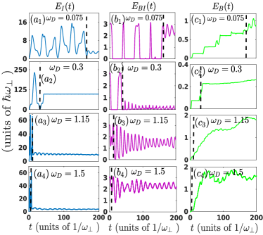
Figure 3: Time-evolution of the individual energy contributions of ($\displaystyle a_{1}$)-($\displaystyle a_{4}$) the impurities $\displaystyle E_{I}(t)$, ($\displaystyle b_{1}$)-($\displaystyle b_{4}$) the interspecies interaction energy $\displaystyle E_{BI}(t)$ and ($\displaystyle c_{1}$)-($\displaystyle c_{2}$) the bosonic bath $\displaystyle E_{B}(t)$ at different driving frequencies $\displaystyle\omega_{D}$ (see legends). The dashed vertical lines mark the time-instant, $\displaystyle t=t_{f}$, of the termination of the shaking. The remaining system parameters are the same as Fig. 1.

The temporal evolution of the above described energy terms is illustrated in Fig. 3 for distinct driving frequencies $\displaystyle\omega_{D}$. As it can be seen, in the course of the shaking i.e. $\displaystyle t<t_{f}$ the energy of the impurities $\displaystyle E_{I}(t)$ overall increases for every $\displaystyle\omega_{D}$ [Figs. 3 ($\displaystyle a_{1}$)-($\displaystyle a_{4}$)] since they are externally driven and therefore their kinetic energy becomes larger. Simultaneously the energy of the bosonic bath $\displaystyle E_{B}(t)$ exhibits an increasing tendency [Figs. 3 ($\displaystyle c_{1}$)-($\displaystyle c_{4}$)] while the impurity-BEC interaction energy $\displaystyle E_{BI}(t)$ decreases [Figs. 3 ($\displaystyle b_{1}$)-($\displaystyle b_{4}$)]. Notice that for low driving frequencies, namely $\displaystyle\omega_{D}=0.075$ and $\displaystyle\omega_{D}=0.3$, when $\displaystyle E_{BI}(t)$ tends to zero signifies that the impurities escape from the bosonic bath [e.g. see Fig. 1 ($\displaystyle b_{1}$) and Fig. 3 ($\displaystyle b_{1}$)] while the subsequent abrupt increase of $\displaystyle E_{BI}(t)$ from zero to a finite value is caused by the re-entering of the impurities into the bath. For instance at $\displaystyle\omega_{D}=0.3$ the impurities remain within the bath in the time-intervals $\displaystyle 0\leq t\leq 6$ and $\displaystyle 24.8\leq t\leq 38.1$ [Fig. 1 ($\displaystyle b_{2}$)], exchanging a small amount of energy with the bath [Fig. 3 ($\displaystyle b_{2}$)], resulting in the negligible increase of the $\displaystyle E_{B}(t)$ [Fig. 3($\displaystyle c_{2}$)]. This behavior of the individual energy contributions suggests an energy transfer process Mistakidis et al. (2019d, a); Lampo et al. (2017); Nielsen et al. (2019) from the impurities to the bosonic gas e.g. imprinted in the density of the latter as a center-of-mass dipole mode. Moreover, after the application of the driving i.e. for $\displaystyle t>t_{f}$, $\displaystyle E_{I}$ is augmented as depicted in Figs. 3 ($\displaystyle a_{1}$)-($\displaystyle a_{4}$) while $\displaystyle E_{B}(t)$ acquires larger values since for $\displaystyle t>t_{f}$ the impurities reside within the BEC and thus convey energy to the latter. In the same time-interval the corresponding interspecies interaction energy $\displaystyle E_{BI}(t)$ shows an oscillatory behavior. In particular, when the impurities travel towards the edge of the bath [see also Fig. 1 ($\displaystyle b_{2}$)] they acquire more kinetic energy, and thus $\displaystyle E_{I}(t)$ increases, and transfer energy to the BEC resulting in an increase of $\displaystyle E_{B}(t)$ while $\displaystyle E_{BI}(t)$ decreases and vice versa. Note also that the impurities possess a maximum energy value in the case of resonant driving $\displaystyle\omega_{D}=\omega$ and as a consequence they are able to move far away from the Thomas-Fermi radius of the BEC [Fig. 1 ($\displaystyle b_{2}$)].

Additionally, at large driving frequencies such as $\displaystyle\omega_{D}=1.15$ and $\displaystyle\omega_{D}=1.5$, the energy gain of the bath is maximum since the impurities remain mostly within the BEC and continuously transfer energy to the latter [see Figs. 3 ($\displaystyle c_{3}$) and ($\displaystyle c_{4}$)]. For this reason also the excitations of the bath are enhanced for such large driving frequencies and its center-of-mass oscillations possess their largest amplitude [Figs. 2 ($\displaystyle a_{3}$) and ($\displaystyle a_{4}$)].

III.4 Development of intra and interspecies correlations

To estimate the degree of intra- and interspecies (entanglement) correlations in the course of the nonequilibrium dynamics of the bosonic mixture we resort to the deviation from unity of the first natural population $\displaystyle\mathcal{F}_{\sigma}(t)$ [Eq. (7)] and the von-Neumann entropy $\displaystyle S_{VN}(t)$ [Eq. (6)] respectively. It is worth mentioning that $\displaystyle\mathcal{F}_{\sigma}(t)>0$ signifies the emergence of $\displaystyle\sigma$-species intraspecies correlations (see also Sec. II.3), while $\displaystyle S_{VN}(t)\neq 0$ indicates the appearance of interspecies entanglement into the system Mistakidis et al. (2018a); Erdmann et al. (2019).

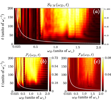
Figure 4: Dynamics of (a) the von-Neumann entropy $\displaystyle S_{VN}(t)$ and the deviation from unity of the first natural population of (b) the impurities $\displaystyle\mathcal{F}_{I}(t)$ and (c) the bosonic gas $\displaystyle\mathcal{F}_{B}(t)$ for varying driving frequency $\displaystyle\omega_{D}$. The white curves indicate the duration $\displaystyle t=t_{f}=4\pi/\omega_{D}$ of the periodic shaking of the potential of the impurities for different driving frequencies $\displaystyle\omega_{D}$.

Figure 4 depicts the dynamics of the von-Neumann entropy $\displaystyle S_{VN}(t)$ and the degree of $\displaystyle\sigma$-species intraspecies correlations $\displaystyle\mathcal{F}_{\sigma}(t)$ for a relevant interval of the driving frequency $\displaystyle\omega_{D}$. For weak and intermediate driving frequencies, i.e. $\displaystyle 0<\omega_{D}<0.7$, and referring to the time-interval of the shaking (see the dashed white line in Fig. 4) the entanglement between the species [Fig. 4 ($\displaystyle a$)] and the impurity-impurity correlations [Fig. 4 ($\displaystyle b$)] are small since $\displaystyle\max[S_{VN}(t<t_{f})]<0.1$ and $\displaystyle\max[\mathcal{F}_{I}(t<t_{f})]<0.12$. However, for later times we observe the build up of finite entanglement at particular values of $\displaystyle\omega_{D}$ and strong impurity-impurity correlations almost for every $\displaystyle 0<\omega_{D}<0.7$. For instance, at $\displaystyle\omega_{D}=0.1$, $\displaystyle S_{VN}(t=10)\approx 0.03$ while $\displaystyle S_{VN}(t=60)\approx 0.24$ and $\displaystyle S_{VN}(t=180)\approx 1.15$ [Fig.4 ($\displaystyle a$)] indicating the growth of entanglement via $\displaystyle S_{VN}(t)$ as time evolves. Similarly, at $\displaystyle\omega_{D}=0.1$, $\displaystyle\mathcal{F}_{I}(t=10)\approx 0.01$ and $\displaystyle\mathcal{F}_{I}(t=60)\approx 0.07$, $\displaystyle\mathcal{F}_{I}(t=180)\approx 0.27$ [Fig.4 ($\displaystyle b$)] designating the development of impurity-impurity correlations during the evolution. Recall that in the resonantly driven region i.e. $\displaystyle 0.2<\omega_{D}<0.45$ the impurities are expelled outside the bosonic bath leading to weak interspecies correlations. Entering the high frequency driving regime, and in particular $\displaystyle 0.75<\omega_{D}<1.7$, both $\displaystyle S_{VN}(t)$ and $\displaystyle\mathcal{F}_{I}(t)$ acquire larger values especially for $\displaystyle t>t_{f}$ indicating the existence of non-negligible interspecies entanglement and impurity intraspecies correlations. Note here that again in the course of the shaking, i.e. $\displaystyle t<t_{f}$, $\displaystyle\max[S_{VN}(t<t_{f})]<0.1$ and $\displaystyle\max[\mathcal{F}_{I}(t<t_{f})]<0.05$ implying that impurity-BEC and impurity-impurity correlations are mainly suppressed. We remark that the interspecies entanglement is maximized in the driving regime $\displaystyle 0.75<\omega_{D}<1.7$ [Fig. 4($\displaystyle a$)] since for such driving frequencies the impurities mostly reside within the bath, see e.g. Figs. 1 ($\displaystyle a_{3}$), ($\displaystyle b_{3}$), and therefore the impurity-BEC overlap is larger as compared to a smaller $\displaystyle\omega_{D}$. Turning to the driving regime $\displaystyle\omega_{D}>1.8$ we can deduce that the degree of the above-mentioned correlations almost vanishes since $\displaystyle\max[S_{VN}(t)]<0.1$ as well as $\displaystyle\max[\mathcal{F}_{I}(t)]<0.05$ during the entire evolution. This can be attributed to the fact that for such a high frequency driving the impurities cannot adapt their motion to the external driving thus remaining to a large extent unperturbed Mistakidis et al. (2015); Mistakidis and Schmelcher (2017); Goldman et al. (2015).

Interestingly, by inspecting $\displaystyle\mathcal{F}_{B}(t)$ [Fig. 4 ($\displaystyle c$)] we can deduce that the intraspecies correlations of the bosonic gas are generally suppressed independently of the driving frequency. Indeed, only in the driving region $\displaystyle 0.75<\omega_{D}<1.7$ we observe a small amount of intraspecies correlations of the bath where $\displaystyle\max[\mathcal{F}_{B}(t)]=0.07$ which occurs around $\displaystyle\omega_{D}=1.475$. Otherwise it mostly holds that $\displaystyle\mathcal{F}_{B}(t)<0.02$ throughout the evolution. This behavior essentially indicates that the first natural population of the bath $\displaystyle\eta^{B}_{1}(t)$ remains close to unity during the time-evolution which can be partly attributed to the considered large number of $\displaystyle N_{B}=100$ particles.

Summarizing, we deduce that for driving frequencies lying in the interval $\displaystyle 0.75<\omega_{D}<1.7$ the dynamics is characterized by a significant amount of both intra- and interspecies correlations [Fig. 4]. As a consequence, a many-body treatment is essential for the adequate description of the dynamics. However, for $\displaystyle 0<\omega_{D}<0.7$ the degree of intraspecies BEC and impurity-BEC correlations is in general supressed while impurity-impurity correlations are finite for $\displaystyle t>t_{f}$ [Fig. 4]. In this sense, the total many-body wavefunction and the wavefunction of the BEC can be well approximated by a mean-field product ansatz, i.e. $\displaystyle\lambda_{1}(t)=1$ in Eq. (3) and $\displaystyle n_{1}^{B}(t)=1$ in Eq. (4). However, the wavefunction of the impurities can not be written as a product state since $\displaystyle n_{i>1}^{I}(t)>0$. Finally, when $\displaystyle\omega_{D}>1.8$ all correlations are mainly vanishing and therefore the driven dynamics of the system can be adequately captured within a corresponding mean-field treatment.

III.5 Spatial coherence

To elucidate further the underlying intraspecies correlation properties of the driven bosonic mixture we investigate the $\displaystyle\sigma$-species one-body coherence function $\displaystyle g_{\sigma}^{(1)}(x,x^{\prime};t)$ Katsimiga et al. (2017b); Mistakidis et al. (2018a); Naraschewski and Glauber (1999) introduced in Eq. (5). Recall that the situation with $\displaystyle g_{\sigma}^{(1)}(x,x^{\prime};t)=1$ signifies that the $\displaystyle\sigma$-species many-body state is identical to a mean-field product ansatz. Therefore, if $\displaystyle g_{\sigma}^{(1)}(x,x^{\prime};t)<1$ indicates the necessity of a beyond mean-field treatment of the dynamics. Figure 5 ($\displaystyle a_{1}$)-($\displaystyle a_{4}$) and ($\displaystyle b_{1}$)-($\displaystyle b_{4}$) present $\displaystyle g^{(1)}_{B}(x,x^{{}^{\prime}},t)$ and $\displaystyle g^{(1)}_{I}(x,x^{{}^{\prime}};t)$ respectively for selected time-instants of the pulse driven dynamics with $\displaystyle\omega_{D}=1.15$. Note here that we focus on large driving frequencies since the degree of correlations is enhanced in this region as we have identified in the previous section III.4, see also Fig. 4.

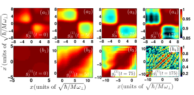
Figure 5: Snapshots of the one-body coherence function $\displaystyle g^{(1)}_{\sigma}(x,x^{\prime};t)$ of ($\displaystyle a_{1}$)-($\displaystyle a_{4}$) the bosonic bath ($\displaystyle\sigma=B$) and $\displaystyle(b_{1})$-$\displaystyle(b_{4})$ the impurities ($\displaystyle\sigma=I$). The dynamics is induced by shaking the harmonic oscillator potential of the impurities at frequency $\displaystyle\omega_{D}=1.15$ until $\displaystyle t=t_{f}=4\pi/\omega_{D}$ i.e. for two periods. All other system parameters are the same as in Fig. 1.

Regarding the bosonic gas, we observe that partial (i.e. very limited) losses of coherence occur between its right ($\displaystyle x>0$) and left ($\displaystyle x>0$) spatial regions since the off-diagonal elements of the coherence function take values smaller than unity, i.e. $\displaystyle g^{(1)}_{B}(x,x^{\prime}\neq x;t)<1$ throughout the evolution, see Figs. 5 ($\displaystyle a_{1}$)-($\displaystyle a_{4}$). Even the initial state of the bath is not perfectly coherent see e.g. $\displaystyle g^{(1)}_{B}(x=4,x^{\prime}=-4;t=0)\approx 0.96$ in Fig. 5 ($\displaystyle a_{1}$). Moreover as time evolves the aforementioned losses of coherence become more prominent, for instance $\displaystyle g^{(1)}_{B}(x=4.0,x^{\prime}=-2.5;t=50)\approx 0.91$ [Fig. 5 ($\displaystyle a_{2}$)] and $\displaystyle g^{(1)}_{B}(x=4.0,x^{\prime}=-2.5;t=175)\approx 0.88$ [Fig. 5 ($\displaystyle a_{4}$)] but remain very limited. It is also worth mentioning that the development of coherence losses in the bath during the dynamics is caused in part by the motion and interaction of the impurities within the BEC since the latter is not directly affected by the driving. Turning to the impurities we can deduce that initially small coherence losses are present between the edges of their cloud, see e.g. $\displaystyle g^{(1)}_{I}(x=4,x^{\prime}=-4;t=0)\approx 0.95$ in Fig. 5 ($\displaystyle b_{1}$). In the course of the time-evolution the shaking introduces a large amount of coherence losses Li and Kuang (2019), e.g. $\displaystyle g^{(1)}_{I}(x=2.8,x^{\prime}=-4.5;t=50)\approx 0.80$ in Fig. 5 ($\displaystyle b_{2}$), which become substantial deeper in the evolution. The latter can be directly inferred from the vanishing tendency of the off-diagonal elements of the one-body coherence function. Indeed, $\displaystyle g^{(1)}_{I}(x=2.8,x^{\prime}=-4.5;t=75)\approx 0.57$ [Fig. 5 ($\displaystyle b_{3}$)] and $\displaystyle g^{(1)}_{I}(x=2.8,x^{\prime}=-4.5;t=175)\approx 0.39$ [Fig. 5 ($\displaystyle b_{4}$)]. We remark that the spatial fluctuations of $\displaystyle g^{(1)}_{I}(x,x^{\prime}\neq x;t)$ at long evolution times [e.g. at $\displaystyle t=175$ in Fig. 5 ($\displaystyle b_{4}$)] are pronounced due to the delocalized shape of the corresponding $\displaystyle\rho^{(1)}_{I}(x;t)$, see Fig. 1 ($\displaystyle b_{3}$). Note also that the amount of coherence losses of the impurities is significantly larger than the corresponding ones occurring for the bosonic gas.

III.6 Effect of the intraspecies interaction of the BEC on the dynamics

To infer whether the intraspecies interaction of the bosonic bath can alter the above-described pulse driven dynamics we next investigate the dynamical response of the system for a specific $\displaystyle\omega_{D}$ and different values of $\displaystyle g_{BB}$. For simplicity, we focus on large driving frequencies e.g. $\displaystyle\omega_{D}=1.5$ where the impurity dynamics shows a more regular behavior [Fig. 1 ($\displaystyle b_{4}$)] compared to a smaller $\displaystyle\omega_{D}$, see for instance Fig. 1 ($\displaystyle b_{2}$), and also the degree of correlations is enhanced [Fig. 4]. Figure 6 presents the resulting time-evolution of the impurities single-particle density $\displaystyle\rho^{(1)}_{I}(x;t)$ for $\displaystyle g_{BB}=0.2$ [Fig. 6 ($\displaystyle a$)] and $\displaystyle g_{BB}=0.8$ [Fig. 6 ($\displaystyle b$)] for $\displaystyle\omega_{D}=1.5$. As it can be seen, for a weakly interacting BEC background the impurities show a relatively dispersive behavior identified by the highly delocalized shape of $\displaystyle\rho^{(1)}_{I}(x;t)$ which becomes very prominent deep in the evolution, see Fig. 6 ($\displaystyle a$). However upon increasing the intraspecies interaction of the bath, $\displaystyle\rho^{(1)}_{I}(x;t)$ undergoes a decaying amplitude oscillatory motion within $\displaystyle\rho^{(1)}_{B}(x;t)$ while possessing a localized shape throughout the evolution as illustrated in Fig. 6 ($\displaystyle b$). Recall that this latter behavior of the impurities for $\displaystyle g_{BB}=0.8$ persists also when $\displaystyle g_{BB}=0.5$ [Fig. 1 ($\displaystyle b_{4}$)]. For weak repulsive interactions such as $\displaystyle g_{BB}=0.2$ and of course the same $\displaystyle N_{B}$ the bosonic bath is more dense and its Thomas-Fermi radius is smaller than for a stronger $\displaystyle g_{BB}$. Accordingly the interatomic distance for a weak $\displaystyle g_{BB}$ is smaller compared to the case of a strong $\displaystyle g_{BB}$ and therefore the impurities experience more scattering events with the atoms of the bath, resulting in the observed dispersive behavior of $\displaystyle\rho^{(1)}_{I}(x;t)$.

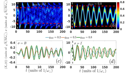
Figure 6: Single-particle density evolution of the two periodically driven impurities with $\displaystyle\omega_{D}=1.5$ for ($\displaystyle a$) $\displaystyle g_{BB}=0.2$ and ($\displaystyle b$) $\displaystyle g_{BB}=0.8$. Dynamics of ($\displaystyle c$) $\displaystyle\langle X_{B}(t)\rangle$ and ($\displaystyle d$) $\displaystyle\langle X_{I}(t)\rangle$ for different intraspecies interaction strengths $\displaystyle g_{BB}$ of the bath (see legend) when $\displaystyle\omega_{D}=1.5$. The external driving of the harmonic oscillator of the impurities is performed up to $\displaystyle t_{f}=4\pi/\omega_{D}$ i.e. for two periods (see the dashed vertical line). The mixture consists of $\displaystyle N_{B}=100$ bosons with $\displaystyle g_{BB}=0.5$ and $\displaystyle N_{I}=2$ interacting $\displaystyle g_{II}=0.4$ impurities being trapped in a harmonic oscillator of frequency $\displaystyle\omega=0.3$. The interspecies repulsion is $\displaystyle g_{BI}=0.2$ and the system is initialized in its ground state. The dashed horizontal lines in ($\displaystyle a$)-($\displaystyle b$) mark the location of the Thomas-Fermi radius of the bosonic gas.

In order to further elucidate the dynamical response of the binary system for distinct values of $\displaystyle g_{BB}$ we also inspect the underlying center-of-mass motion of both the bosonic bath $\displaystyle\langle X_{B}(t)\rangle$ [Fig. 6 ($\displaystyle c$)] and the impurities $\displaystyle\langle X_{I}(t)\rangle$ [Fig. 6 ($\displaystyle d$)]. Regarding the impurities we observe that $\displaystyle\langle X_{I}(t)\rangle$ performs a decaying amplitude single-frequency oscillatory motion independently of $\displaystyle g_{BB}$. Additionally, the oscillation amplitude of $\displaystyle\langle X_{I}(t)\rangle$ is smaller and its decay is more dramatic for a decreasing $\displaystyle g_{BB}$, see Fig. 6 ($\displaystyle d$). Indeed, the Thomas-Fermi radius of the BEC reduces for a smaller $\displaystyle g_{BB}$, e.g. $\displaystyle R_{TF}\approx 6.5$ for $\displaystyle g_{BB}=0.2$ and $\displaystyle R_{TF}\approx 9.5$ when $\displaystyle g_{BB}=0.8$. As a consequence the oscillation amplitude of $\displaystyle\langle X_{I}(t)\rangle$ is smaller for a decreasing $\displaystyle g_{BB}$ since for such high frequency drivings the impurities oscillate within the bosonic bath whose size becomes smaller. On the other hand, the center-of-mass of the bosonic bath as already explained in Secs. III.1 and III.2 undergoes an irregular oscillatory behavior due to the collective dipole mode caused by the motion of the impurities inside the bath. Here we can infer that the oscillation amplitude of $\displaystyle\langle X_{B}(t)\rangle$ is mainly increased for a stronger $\displaystyle g_{BB}$ as in the case of $\displaystyle\langle X_{I}(t)\rangle$, see Fig. 6 ($\displaystyle d$). However this behavior is not valid in general and notable exceptions occur during the evolution.

IV Pulse driven dynamics of immiscible components

Having analyzed in detail the driven dynamics of two miscible species whose interactions satisfy the condition $\displaystyle g^{2}_{BI}\leq g_{II}g_{BB}$ Ao and Chui (1998); Timmermans (1998) we then discuss the corresponding nonequilibrium dynamics initializing the binary system in an immiscible state. As in Sec. III, the highly imbalanced mixture comprises of $\displaystyle N_{B}=100$ bosons and $\displaystyle N_{I}=2$ impurities and both species are trapped in the same harmonic potential with $\displaystyle\omega=0.3$. In order to realize an immiscible initial configuration we consider the same intraspecies interactions as before, namely $\displaystyle g_{BB}=0.5$ and $\displaystyle g_{II}=0.4$, but a stronger interspecies repulsion $\displaystyle g_{BI}=1.0$ such that the immiscibility condition $\displaystyle g^{2}_{BI}\geq g_{II}g_{BB}$ is satisfied. The system is initially prepared into its many-body ground state where the single-particle densities of the individual species are spatially phase separated as shown in Fig. 7 (a). In particular, $\displaystyle\rho^{(1)}_{B}(x)$ resides around the trap center while $\displaystyle\rho^{(1)}_{I}(x)$ forms a two density hump structure with each hump located at an edge of the Thomas-Fermi radius, $\displaystyle R_{TF}\approx 8.3$, of the bosonic gas.

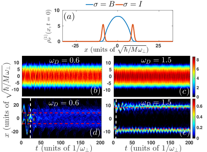
Figure 7: (a) Ground state single-particle density profiles $\displaystyle\rho^{(1)}_{\sigma}(x)$ of the bosonic gas ($\displaystyle\sigma=B$) and the impurities ($\displaystyle\sigma=I$). Evolution of (b), (c) $\displaystyle\rho^{(1)}_{B}(x;t)$ and (d), (e) $\displaystyle\rho^{(1)}_{I}(x;t)$ for different driving frequencies (see legends). The periodic driving of the impurities harmonic oscillator is maintained up to $\displaystyle t_{f}=4\pi/\omega_{D}$ (see the dashed vertical lines) and then the system evolves freely. The harmonically trapped ($\displaystyle\omega=0.3$) bosonic mixture comprises of $\displaystyle N_{B}=100$ atoms and $\displaystyle N_{I}=2$ impurities with intra- and interspecies repulsions $\displaystyle g_{BB}=0.5$, $\displaystyle g_{II}=0.4$ and $\displaystyle g_{BI}=1.0$ respectively and it is prepared in its ground state. The dashed horizontal lines in ($\displaystyle d$), ($\displaystyle e$) indicate the location of the Thomas-Fermi radius of the bosonic gas while the grey dashed rectangle in ($\displaystyle d$) marks the bunching of the impurities around $\displaystyle x=0$.

The nonequilibrium dynamics is induced by considering a pulse shaking of the impurities harmonic oscillator described by Eq. (2) where the system is periodically driven for two driving periods, $\displaystyle t_{f}=4\pi/\omega_{D}$, and then is left to evolve without any external perturbation. The driving amplitude is $\displaystyle\mathcal{A}=20\gg R_{TF}$. For simplicity we study below the cases of large driving frequencies namely $\displaystyle\omega_{D}=0.6$ and $\displaystyle\omega_{D}=1.5$ since for weak $\displaystyle\omega_{D}<0.5$ the resulting dynamics of the impurities is found to be highly dispersive i.e. $\displaystyle\rho^{(1)}_{I}(x;t)$ exhibits a strongly delocalized behavior within and outside the BEC background (results not shown here for brevity). Note also that the driving frequencies $\displaystyle\omega_{D}=0.6$ and $\displaystyle\omega_{D}=1.5$ are representative of the so-called intermediate and high frequency driving regimes respectively.

Figures 7 (b), (d) and (c), (e) depict the time-evolution of the $\displaystyle\sigma$-species single-particle density following a periodic driving with $\displaystyle\omega_{D}=0.6$ and $\displaystyle\omega_{D}=1.5$ respectively. For $\displaystyle\omega_{D}=0.6$ and referring to $\displaystyle t<t_{f}=20.9$ (see the dashed line in Fig. 7 (d)) we observe that both density humps of $\displaystyle\rho^{(1)}_{I}(x;t)$ ensue their external trap until it reaches for the first time its maximum displacement $\displaystyle\mathcal{A}$. Then as the harmonic oscillator turns towards $\displaystyle x=0$ the density humps collide while emitting small amplitude density fragments due to their interaction with the atoms of the bath and at $\displaystyle t=t_{f}$ $\displaystyle\rho^{(1)}_{I}(x;t)$ is predominantly concentrated at the origin $\displaystyle x=0$, see the grey dashed rectangle in Fig. 7 ($\displaystyle d$). Subsequently, for $\displaystyle t>t_{f}$, the impurities are predominantly trapped into $\displaystyle\rho^{(1)}_{B}(x;t)$ throughout the dynamics and therefore the species are completely mixed. In particular, $\displaystyle\rho^{(1)}_{I}(x;t)$ shortly after $\displaystyle t_{f}$ exhibits a delocalized behavior [Fig. 7 (d)] inside $\displaystyle\rho^{(1)}_{B}(x;t)$ while for $\displaystyle t>120$ it shows a tendency to segregate into two fragments symmetrically placed around $\displaystyle x=0$ and being located around the edges of the BEC background [Fig. 7 ($\displaystyle b$)]. Moreover the motion of the impurities within $\displaystyle\rho^{(1)}_{B}(x;t)$ perturb the bath which in turn performs a collective dipole motion [Fig. 7 (b)]. It is worth noticing here that besides the inherent tendency of the two species to remain spatially separated due to the strong $\displaystyle g_{BI}$, the driving enforces the impurities to infuse into the BEC in the course of dynamics [Fig. 7 ($\displaystyle d$)].

In contrast to the above-described mixing dynamics, a sufficiently high frequency driving e.g. $\displaystyle\omega_{D}=1.5$ [see Figs. 7 ($\displaystyle c$), ($\displaystyle e$)] preserves the phase separation in the course of the evolution even after $\displaystyle t=t_{f}=8.37$. Indeed, the initial density humps of $\displaystyle\rho^{(1)}_{I}(x;t)$ remain while oscillating at the edges of the bosonic gas throughout the dynamics. Interestingly, the structures building upon each density hump of $\displaystyle\rho^{(1)}_{I}(x;t)$ are not identical, for instance $\displaystyle\rho^{(1)}_{I}(x)$ is fragmented in the upper ($\displaystyle x>0$) hump within $\displaystyle 22<t<45$ but not in the lower ($\displaystyle x<0$) one [Fig. 7 ($\displaystyle e$)]. This difference is caused by the location of each density hump at $\displaystyle t=t_{f}$. Indeed the upper hump at $\displaystyle t=t_{f}$ resides within the bath and therefore it interacts with the latter while the lower hump lies at the edge of the BEC thus hardly interacting with it. On the other hand, the bosonic gas due to its collisions with $\displaystyle\rho^{(1)}_{I}(x;t)$ at the edges of $\displaystyle\rho^{(1)}_{B}(x;t)$ undergoes a dipole motion [Fig. 7 (c)].

We also remark here that an energy transfer process from the impurities to the bosonic bath occurs in both driving scenarios (results not shown here for brevity). Here, the energy gain of the bath is significantly enhanced for $\displaystyle\omega_{D}=0.6$ where the components are miscible during the evolution while for $\displaystyle\omega_{D}=1.5$ $\displaystyle E_{B}(t)$ mainly increases for $\displaystyle t<t_{f}$ since the components overlap and remains almost constant for $\displaystyle t>t_{f}$ where the immiscibility is preserved. Additionally, let us note in passing that a similar overall phenomenology regarding the dynamical response of both the bosonic bath and the impurities takes place for a continuous shaking of the impurities harmonic oscillator (results not shown for brevity).

V Continuous shaking of the trap potential

Next, we unravel the emergent nonequilibrium dynamics of the binary bosonic system when considering that the periodic driving of the harmonic trap of the impurities is maintained throughout the evolution and not for just two periods of the pulse driving as in Sec. III. The system parameters are the same as in the previous Sec. III, namely the bath comprises of $\displaystyle N_{B}=100$ bosons with $\displaystyle g_{BB}=0.5$ and $\displaystyle N_{I}=2$ impurities where $\displaystyle g_{II}=0.4$. The impurity-BEC interaction is $\displaystyle g_{BI}=0.2$ and thus the species are initially ($\displaystyle t=0$) miscible. Both species are trapped in a harmonic oscillator of frequency $\displaystyle\omega=0.3$ and the system is initialized in its many-body ground state. Subsequently, from $\displaystyle t=0$ on, the harmonic oscillator of the impurities is periodically driven [see Eq. (2)] for the entire time-evolution. The oscillation amplitude is assumed to be $\displaystyle\mathcal{A}=20\gg R_{TF}\approx 8.3$.

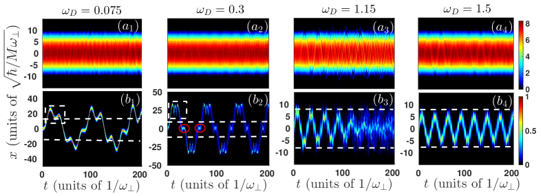
Figure 8: Dynamics of the $\displaystyle\sigma$-species single-particle density $\displaystyle\rho^{(1)}_{\sigma}(x;t)$ of ($\displaystyle a_{1}$)-($\displaystyle a_{4}$) the bosonic bath ($\displaystyle\sigma=B$) and ($\displaystyle b_{1}$)-($\displaystyle b_{4}$) the two impurities ($\displaystyle\sigma=I$) for selected shaking frequencies $\displaystyle\omega_{D}$ (see legends). The shaking of the harmonic oscillator potential of the impurities is maintained throughout the evolution. The system contains $\displaystyle N_{B}=100$ bosons and $\displaystyle N_{I}=2$ impurities with intra- and interspecies interactions $\displaystyle g_{BB}=0.5$, $\displaystyle g_{II}=0.4$ and $\displaystyle g_{BI}=0.2$ respectively. It is confined in a harmonic trap of frequency $\displaystyle\omega=0.3$ and it is initialized into its ground state. The dashed horizontal lines in ($\displaystyle b_{1}$)-($\displaystyle b_{4}$) indicate the location of the Thomas-Fermi radius of the bosonic bath. The white dashed rectangles in ($\displaystyle b_{1}$), ($\displaystyle b_{2}$) and the red circles in ($\displaystyle b_{2}$) mark specific back-scattering events of the impurities during the driving.

V.1 Dynamics of the single-particle density and the center-of-mass

To visualize the nonequilibrium dynamics of the system subjected to a continuous shaking we resort to the time-evolution of the single-particle density and the position of the center-of-mass of the $\displaystyle\sigma$-species presented in Fig. 8 and Fig. 9 respectively for selective driving frequencies as in Sec. III. Focusing on low driving frequencies e.g. $\displaystyle\omega_{D}=0.075$ the impurities perform an “irregular” oscillatory motion overall following their driven potential [Fig. 8 ($\displaystyle b_{1}$)]. Note that the observed dynamical response of the impurities is reminiscent of the corresponding response of the case of pulse driving for $\displaystyle t<t_{f}$ (i.e. before its termination) discussed in Sec. III, see also Fig. 1 ($\displaystyle b_{1}$). Importantly, here, the motion taking place during the first oscillation period of the external potential is periodically repeated within each driving cycle [Figs. 8 ($\displaystyle b_{1}$)]. This behavior of the impurities is also imprinted in their trajectory presented in Fig. 9 ($\displaystyle b_{1}$). We remark that this time periodic behavior of $\displaystyle\rho^{(1)}_{I}(x;t)$ is caused by the continuous driving and it is in contrast to the pulse driven case where after the termination of the driving the impurities oscillate well inside the bosonic medium, see also Fig. 1 ($\displaystyle b_{1}$). Also note here that due to the continuous driving the oscillation amplitude of $\displaystyle\rho^{(1)}_{I}(x;t)$ is slightly increased every driving period, e.g. $\displaystyle\rho^{(1)}_{I}(x,t=99)$ reaches $\displaystyle x=29.5$ while it is located at $\displaystyle x=33.4$ when $\displaystyle t=182.5$ [Fig. 8 ($\displaystyle b_{1}$)]. Moreover, the BEC background $\displaystyle\rho^{(1)}_{B}(x;t)$ shows weak distortions from its initial Thomas-Fermi profile being imprinted as a small amplitude collective dipole motion [Fig. 8 ($\displaystyle a_{1}$)] during the dynamics. This latter motion is directly captured by the time-evolution of the center-of-mass which exhibits multifrequency oscillations as shown in Fig. 9 ($\displaystyle a_{1}$).

For resonant driving frequencies, i.e. $\displaystyle\omega_{D}=\omega=0.3$, the impurities exhibit an oscillatory behavior moving inside and outside the bosonic bath [Fig. 8 ($\displaystyle b_{2}$)] during the dynamics. Initially they move towards the left edge of the BEC, escaping from the latter at $\displaystyle t\approx 20.2$, and reach $\displaystyle x\approx 33.6$ where they experience during their motion two back-scattering events due to the external driving [see the white dashed rectangle in Fig. 8 ($\displaystyle b_{2}$)]. Later on they penetrate the BEC background interacting with its atoms and featuring a dramatic back-scattering event at $\displaystyle x\approx 0$ manifested by the prominent density hump of $\displaystyle\rho^{(1)}_{I}(x;t)$ [see the red circle in Fig. 8 ($\displaystyle b_{2}$)]. This behavior suggests that the impurities slow down at this location and bunch momentarily before moving to the opposite edge of the bath. Afterwards the impurities undergo a similar to the above-described dynamical behavior, i.e. moving outside the right edge of the BEC and being reflected backwards, until the first driving period is completed. As time evolves the impurities repeat the same pattern within every driving period, see Fig. 8 ($\displaystyle b_{2}$). Indeed, inspecting the trajectory of the impurities shown in Fig. 9 ($\displaystyle b_{2}$) we can directly infer their oscillatory behavior characterized by a slightly decaying amplitude. The latter signals the dissipation of energy into the bosonic bath as we shall argue in the following section. We remark that compared to the pulse driving case the dynamical response of the impurities remains the same for $\displaystyle t<t_{f}$ but it is significantly altered for $\displaystyle t>t_{f}$ where the driving is terminated and the impurities are mainly deposited outside the edge of the bath throughout the evolution [Figs. 1 ($\displaystyle b_{1}$)]. On the other hand the shape of the bosonic single-particle density is to a large extent unperturbed, see Fig. 8 ($\displaystyle a_{2}$), because the impurities reside majorly outside of $\displaystyle\rho^{(1)}_{I}(x;t)$. However, the disturbances caused by the motion of the impurities within the bosonic bath are imprinted into the latter as a collective dipole mode identified by the oscillatory behavior of $\displaystyle\langle X_{B}(t)\rangle$ depicted in Fig. 9 ($\displaystyle a_{2}$). Interestingly the oscillation amplitude of $\displaystyle\langle X_{B}(t)\rangle$ is amplified over time, a behavior that stems from the continuous nature of the driving Mistakidis et al. (2015); Mistakidis and Schmelcher (2017); Goldman et al. (2015).

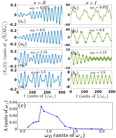
Figure 9: Evolution of the center-of-mass of ($\displaystyle a_{1}$)-($\displaystyle a_{4}$) the bath $\displaystyle\langle X_{B}(t)\rangle$ and ($\displaystyle b_{1}$)-($\displaystyle b_{4}$) the impurities $\displaystyle\langle X_{I}(t)\rangle$ at distinct driving frequencies $\displaystyle\omega_{D}$ (see legends). ($\displaystyle c$) Damping rate, $\displaystyle\lambda$, of $\displaystyle\langle X_{I}(t)\rangle$ with varying driving frequency for $\displaystyle\omega_{D}>0.6$. The shaking of the impurities is maintained for the entire evolution. The Thomas-Fermi radius of the bosonic gas is $\displaystyle R_{TF}\approx 8.3$. Other system parameters are the same as in Fig. 8.

Consequently we inspect the impurities dynamics for large driving frequencies, namely $\displaystyle\omega_{D}\gg\omega$. Here due to the fast shaking of the harmonic oscillator it is very difficult for the impurities to instantaneously follow their external potential and as a result their motion is restricted to a spatial region which is smaller than the actual driving amplitude $\displaystyle\mathcal{A}$. The resulting time-evolution of $\displaystyle\rho^{(1)}_{I}(x,t)$ is presented in Figs. 8 ($\displaystyle b_{3}$) and ($\displaystyle b_{4}$) for driving frequencies $\displaystyle\omega_{D}=1.15$ and $\displaystyle\omega_{D}=1.5$ respectively. As it can be seen, $\displaystyle\rho^{(1)}_{I}(x;t)$ performs in both cases a decaying amplitude oscillatory motion within the bosonic bath throughout the dynamics. This dynamical response of the impurities is also evident in the time-evolution of their trajectory shown in Figs. 9 ($\displaystyle b_{3}$), ($\displaystyle b_{4}$). Additionally we can deduce that the decay of the oscillation amplitude of the impurities is more pronounced for $\displaystyle\omega_{D}=1.15$ than $\displaystyle\omega_{D}=1.5$, a behavior that is clearly captured in both the dynamics of $\displaystyle\rho^{(1)}_{I}(x;t)$ [Figs. 8 ($\displaystyle b_{3}$), ($\displaystyle b_{4}$)] and the impurities trajectory [Figs. 9 ($\displaystyle b_{3}$), ($\displaystyle b_{4}$)]. We remark that the larger decay amplitude e.g. of $\displaystyle\braket{X_{I}(t)}$ for $\displaystyle\omega_{D}=1.15$ compared to $\displaystyle\omega_{D}=1.5$ is caused by the enhanced degree of interspecies correlations in the former case leading to a faster dephasing of the underlying many-body state, see also Fig. 11 ($\displaystyle a$) and the discussion below. It is also worth mentioning that for $\displaystyle\omega_{D}=1.15$ and referring to the initial stages of the dynamics $\displaystyle\rho^{(1)}_{I}(x;t)$ possesses a localized distribution. However deeper in the evolution, $\displaystyle t>100$ in Fig. 8 ($\displaystyle b_{3}$), where the impurities feature multiple collisions with the atoms of the bosonic gas, $\displaystyle\rho^{(1)}_{I}(x;t)$ exhibits a rather delocalized shape. Interestingly for even larger driving frequencies, e.g. $\displaystyle\omega_{D}=1.5$, $\displaystyle\rho^{(1)}_{I}(x;t)$ exhibits a relatively localized configuration. We remark that compared to the pulse driving scenario [Figs. 1 ($\displaystyle b_{3}$), ($\displaystyle b_{4}$)] the impurities exposed to a continuous shaking remain to a larger extent trapped inside their host during the evolution and the decay of their oscillation amplitude is more pronounced, see e.g. Fig. 2 ($\displaystyle b_{3}$) and Fig. 9 ($\displaystyle b_{3}$). Moreover as a result of the motion of the impurities within the bosonic gas density dips build upon $\displaystyle\rho^{(1)}_{B}(x;t)$ [Figs. 8 ($\displaystyle a_{3}$), ($\displaystyle a_{4}$)] at the instantaneous location of the density humps of $\displaystyle\rho^{(1)}_{I}(x;t)$. Notice that these density dips of $\displaystyle\rho^{(1)}_{B}(x;t)$ become very shallow for $\displaystyle\omega_{D}=1.5$. Overall, the bosonic medium undergoes a multifrequency dipole motion which is captured by its center-of-mass motion presented in Figs. 9 ($\displaystyle a_{3}$), ($\displaystyle a_{4}$). Also, here the amplitude of this dipole motion seems quite insensitive to the driving frequency, compare Figs. 9 ($\displaystyle a_{3}$) and ($\displaystyle a_{4}$).

We have identified that the impurities subjected to a continuous shaking of their harmonic trap remain completely trapped in their host only for large driving frequencies, and in particular for $\displaystyle\omega_{D}>0.6$. As a result, we are able to model the decaying motion of the impurities inside the bosonic medium according to the well-known effective damped equation of motion

$$\ddot{x}+\lambda\dot{x}+\omega^{2}_{\rm eff}x=F_{0}\sin(\omega_{D}t).$$ (9)

In this expression, $\displaystyle\lambda$ is the damping parameter of the impurities, $\displaystyle\omega_{eff}$ denotes the effective trapping due to the presence of the bath and the external harmonic confinement. $\displaystyle F_{0}=\mathcal{A}\omega_{eff}^{2}$ is the amplitude of the external driving force. Moreover, by solving Eq. 9 it can be easily shown that the mean position of the impurities reads

$$\begin{split}\braket{X_{I}(t)}&=e^{-\frac{\lambda}{2}t}\bigg{[}x_{0}\cos(\omega_{0}t)+\frac{u_{0}+\frac{\lambda}{2}x_{0}}{\omega_{0}}\\ &\times\sin(\omega_{0}t)\bigg{]}+\frac{F_{0}\sin(\omega_{D}t+\delta)}{(\omega^{2}_{\rm eff}-\omega^{2}_{D})^{2}+\omega_{D}^{2}\lambda^{2}},\end{split}$$ (10)

where $\displaystyle\omega_{0}=\sqrt{(\omega_{\rm eff})^{2}-\big{(}\frac{\lambda}{2}\big{)}^{2}}$, $\displaystyle x_{0}\equiv\braket{\Psi(0)}{\hat{x}}{\Psi(0)}$, $\displaystyle u_{0}=\mathcal{A}\omega_{D}$ and $\displaystyle\delta$ is a phase factor. Evidently, in this equation the unknown parameters are $\displaystyle\lambda$, $\displaystyle\omega_{\rm eff}$ and $\displaystyle\delta$. In order to determine these parameters we perform a fitting of the analytical form of $\displaystyle\braket{X_{I}(t)}$ provided by Eq. 10 with the numerically obtained result of $\displaystyle\braket{X_{I}(t)}$. Figure 9 ($\displaystyle c$) shows the value of the damping term $\displaystyle\lambda$ obtained through the above-described fitting procedure with respect to the driving frequency. We observe that $\displaystyle\lambda$ increases within the interval $\displaystyle\omega_{D}\in\{0.6,0.85\}$ and subsequently shows an overall decreasing tedency. This behavior of $\displaystyle\lambda$ is also in line with the growth of the average degree of interspecies correlations captured by $\displaystyle\bar{S}_{VN}\equiv(1/T)\int_{0}^{T}dtS_{VN}(t)$. The latter increases for $\displaystyle\omega_{D}\in\{0.6,0.85\}$ and afterwards decreases, see also Fig. 11 ($\displaystyle a$). Accordingly, for $\displaystyle\omega_{D}>1.5$ where $\displaystyle\bar{S}_{VN}\to 0$ also $\displaystyle\lambda\to 0$.

V.2 Energy exchange processes

In order to infer whether impurity-BEC energy transfer mechanisms Lampo et al. (2017); Mistakidis et al. (2019e, c) occur in the course of the continuously driven dynamics we inspect the underlying intra- and interspecies energy terms, namely the energy of the bath $\displaystyle E_{B}(t)$ and the impurities $\displaystyle E_{I}(t)$ as well as the interspecies interaction energy $\displaystyle E_{BI}(t)$ introduced in Sec. III.3. Figure 10 illustrates the dynamics of the above-mentioned energy contributions for different driving frequencies. We can deduce that independently of $\displaystyle\omega_{D}$ the energy of the impurities $\displaystyle E_{I}(t)$ shows an oscillatory behavior [Figs. 10 ($\displaystyle a_{1}$)-($\displaystyle a_{4}$)] whilst the energy of the bosonic bath $\displaystyle E_{B}(t)$ overall increases [Figs. 10 ($\displaystyle c_{1}$)-($\displaystyle c_{4}$)]. More precisely, for a larger $\displaystyle\omega_{D}$ the oscillatory pattern of $\displaystyle E_{I}(t)$ involves a larger number of frequencies [see Fig. 10 ($\displaystyle a_{1}$) and Fig. 10 ($\displaystyle a_{4}$)] and the increase of $\displaystyle E_{B}(t)$ becomes more enhanced, e.g. compare Fig. 10 ($\displaystyle c_{1}$) with Fig. 10 ($\displaystyle c_{4}$). We remark that the oscillations of $\displaystyle E_{I}(t)$ essentially reflect the impurities motion and in particular when they move to the edge of the BEC they possess a larger kinetic energy than if they are close to the trap center, resulting in an increasing tendency of $\displaystyle E_{I}(t)$. Notice also that $\displaystyle E_{I}(t)$ maximizes for $\displaystyle\omega_{D}=\omega$ Goldman and Dalibard (2014); Goldman et al. (2015); Mistakidis et al. (2015) which explains the fact that the impurities exhibit the larger oscillation amplitude [Fig. 9 ($\displaystyle b_{2}$)].

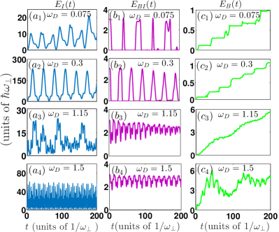
Figure 10: Time-evolution of ($\displaystyle a_{1}$)-($\displaystyle a_{4}$) the energy of the impurities $\displaystyle E_{I}(t)$, ($\displaystyle b_{1}$)-($\displaystyle b_{4}$) the interspecies interaction energy $\displaystyle E_{BI}(t)$ and $\displaystyle(c_{1})$-($\displaystyle c_{2}$) the energy of the bath $\displaystyle E_{B}(t)$ at distinct driving frequencies $\displaystyle\omega_{D}$ (see legends). The shaking of the harmonic oscillator of the impurities is maintained throughout the dynamics. The remaining system parameters are the same as in Fig. 8.

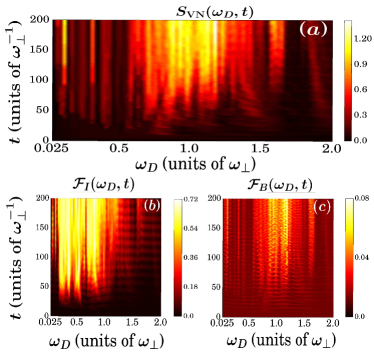
Figure 11: Temporal-evolution of (a) the von-Neumann entropy $\displaystyle S_{VN}(t)$ and the deviation from unity of the first natural population of (b) the impurities $\displaystyle\mathcal{F}_{I}(t)$ and (c) the bosonic gas $\displaystyle\mathcal{F}_{B}(t)$ as a function of the driving frequency $\displaystyle\omega_{D}$. The harmonic oscillator of the two impurities is subjected to a continuous shaking. The remaining system parameters are the same as in Fig. 8.

Most importantly, the simultaneous enhancement of $\displaystyle E_{B}(t)$ accompanied by a reduction of $\displaystyle E_{BI}(t)$ [Figs. 10 ($\displaystyle b_{1}$)-($\displaystyle b_{4}$)] indicates the dissipation of energy from the impurity to its BEC background Mistakidis et al. (2019d, e); Nielsen et al. (2019) manifested in the density of the latter as a collective dipole motion. Additionally it is worth commenting that $\displaystyle E_{BI}(t)$ shows a significantly distinct behavior for low and high driving frequencies. For instance, in the former case $\displaystyle E_{BI}(t)$ becomes zero at specific time-intervals [Fig. 10 ($\displaystyle b_{2}$)] where the impurities escape from the bosonic gas [Fig. 8 ($\displaystyle b_{2}$)] and as a consequence $\displaystyle E_{B}(t)$ shows a constant plateau in the same time frame [Figs. 10 ($\displaystyle c_{1}$), ($\displaystyle c_{2}$)]. However for fast drivings $\displaystyle E_{BI}(t)$ performs irregular oscillations while remaining finite throughout the evolution [Fig. 10 ($\displaystyle b_{4}$)] since the impurities reside well inside the BEC background [Fig. 8 ($\displaystyle b_{4}$)].

V.3 Intra and interspecies correlations

To testify the importance of beyond mean-field intra- and interspecies correlations during the evolution of the system we next employ $\displaystyle\mathcal{F}_{\sigma}(t)$ [Eq. (7)] and $\displaystyle S_{VN}(t)$ [Eq. (6)] respectively. Recall that $\displaystyle\mathcal{F}_{\sigma}(t)>0$ indicates the existence of $\displaystyle\sigma$-species intraspecies correlations and $\displaystyle S_{VN}(t)\neq 0$ designates the occurrence of interspecies ones Mistakidis et al. (2018a, 2019d). Figure 11 showcases both $\displaystyle S_{VN}(t)$ and $\displaystyle\mathcal{F}_{\sigma}(t)$ for a wide range of $\displaystyle\omega_{D}$. Evidently, for short evolution times $\displaystyle t<40$ both intra- and interspecies correlations of the system are suppressed since $\displaystyle\mathcal{F}_{\sigma}(t)$ and $\displaystyle S_{VN}(t)$ deviate only slightly from zero, e.g. $\displaystyle\mathcal{F}_{B}(t=20)\approx 0.015$, $\displaystyle\mathcal{F}_{I}(t=20)\approx 0.02$ and $\displaystyle S_{VN}(t=20)\approx 0.04$ at $\displaystyle\omega_{D}=0.1$. However for $\displaystyle t>40$ we observe a significant development of impurity-BEC [Fig. 11 ($\displaystyle a$)] and impurity-impurity [Fig. 11 ($\displaystyle b$)] correlations while the intraspecies correlations of the bosonic gas remain adequately small for every $\displaystyle\omega_{D}$ [Fig. 11 ($\displaystyle c$)]. Indeed, the largest value of $\displaystyle\mathcal{F}_{B}(t)$ occurs around $\displaystyle\omega_{D}=1.25$ where $\displaystyle\mathcal{F}_{B}(t=180)\approx 0.07$. In particular the impurity-BEC and impurity-impurity correlations, as captured via $\displaystyle S_{VN}(t)$ and $\displaystyle\mathcal{F}_{I}(t)$, are maximized in the range $\displaystyle 0.6<\omega_{D}<1.7$ and $\displaystyle 0.1<\omega_{D}<1.5$ respectively. The predominantly negligible entanglement for $\displaystyle\omega_{D}<0.3$ can be attributed to the fact that the impurities majorly lie outside of the BEC background in the course of the evolution. Note also here that despite the weak entanglement the impurities appear to be strongly correlated for these driving frequencies. Furthermore, for $\displaystyle 0.6<\omega_{D}<1.7$ [Fig. 11($\displaystyle a$)] the impurities are trapped within the bath throughout the evolution [Fig. 8 ($\displaystyle b_{4}$)], testifying the increasing tendency of $\displaystyle S_{VN}(t)$ compared to other values of $\displaystyle\omega_{D}$. At $\displaystyle\omega_{D}>1.7$ both $\displaystyle S_{VN}(t)$ and $\displaystyle\mathcal{F}_{I}(t)$ acquire very small values, a behavior that is attributed to the high frequency driving where the impurities motion cannot be synchronized with the external driving.

Figure 12: One-body coherence function $\displaystyle g^{(1)}_{\sigma}(x,x^{\prime};t)$ of ($\displaystyle a_{1}$)-($\displaystyle a_{4}$) the bosonic bath and ($\displaystyle b_{1}$)-($\displaystyle b_{4}$) the impurities at specific time-instants of the evolution (see legends). The dynamics is induced by a continuous shaking of the harmonic oscillator potential of the impurities at a driving frequency $\displaystyle\omega_{D}=1.15$. The remaining system parameters are the same as in Fig. 8.

In view of the above, for $\displaystyle 0.6<\omega_{D}<1.7$ intra- and interspecies correlations are finite testifying the necessity of a beyond mean-field treatment of the dynamics. For $\displaystyle\omega_{D}<0.7$ since $\displaystyle S_{VN}(t)$ and $\displaystyle\mathcal{F}_{B}(t)$ are suppressed a corresponding product state on the species and the BEC level constitutes an adequate approximation. However, the impurities wavefunction is a superposition of the different single-particle states due to $\displaystyle\mathcal{F}_{I}(t)>0$. Finally, for $\displaystyle\omega_{D}>1.7$ all interparticle correlations almost vanish and therefore the dynamics of the mixture can be modeled to a good approximation within a corresponding mean-field treatment, i.e. $\displaystyle\lambda_{1}(t)=1$ in Eq. (3) and $\displaystyle n_{1}^{B}(t)=n_{1}^{I}=1$ in Eq. (4).

V.4 Coherence losses

Subsequently, we unravel losses of the $\displaystyle\sigma$-species spatial coherence Naraschewski and Glauber (1999); Mistakidis et al. (2018a, 2019d); Katsimiga et al. (2017b) by invoking the corresponding one-body coherence function $\displaystyle g_{\sigma}^{(1)}(x,x^{\prime};t)$ [Eq. (5)]. As in Sec. III.5 we showcase the case of a large driving frequency, $\displaystyle\omega_{D}=1.15$, due to the significant role of correlations in this driving regime compared to the others, see also Fig. 11. Snapshots of $\displaystyle g^{(1)}_{B}(x,x^{\prime},t)$ and $\displaystyle g^{(1)}_{I}(x,x^{\prime};t)$ are shown in Figs. 12 ($\displaystyle a_{1}$)-($\displaystyle a_{4}$) and ($\displaystyle b_{1}$)-($\displaystyle b_{4}$) respectively. Closely inspecting $\displaystyle g^{(1)}_{B}(x,x^{{}^{\prime}},t)$ we can infer that only very small coherence losses take place between the spatial regions $\displaystyle 0<x<6$ and $\displaystyle-6<x^{\prime}<0$. These losses of coherence are almost negligible for $\displaystyle t<50$, e.g. $\displaystyle g^{(1)}_{B}(x=5,x^{\prime}=-1,t=50)\approx 0.97$ in Fig. 12 ($\displaystyle a_{2}$), and later on become relatively pronounced, see e.g. $\displaystyle g^{(1)}_{B}(x=5,x^{\prime}=-6,t=175)\approx 0.82$ in Fig. 12 ($\displaystyle a_{4}$). Note that this behavior of $\displaystyle g^{(1)}_{B}(x,x^{\prime},t)$ is in line with the suppressed degree of intraspecies correlations of the bath presented in Fig. 11 ($\displaystyle c$). Also, the amount of coherence losses is slightly increased when compared to the pulse driving scenario [Figs. 5 ($\displaystyle a_{1}$)-($\displaystyle a_{4}$)]. Regarding the impurities we observe that at $\displaystyle t=0$ they are almost perfectly coherent since $\displaystyle g^{(1)}_{I}(x,x^{\prime};t=0)>0.98$ for every $\displaystyle x$, $\displaystyle x^{\prime}$. However as time evolves a systematic build up of coherence losses Li and Kuang (2019) for $\displaystyle x\neq x^{\prime}$ occurs, e.g. $\displaystyle g^{(1)}_{I}(x=2,x^{\prime}=3;t=50)\approx 0.95$ in Fig. 12 ($\displaystyle b_{2}$), which becomes enhanced for longer times, e.g. $\displaystyle g^{(1)}_{I}(x=2;x^{\prime}=-2;t=150)\approx 0.18$ [Fig. 12 ($\displaystyle b_{3}$)] and $\displaystyle g^{(1)}_{I}(x=2.5,x^{\prime}=-2.5;t=175)\approx 0.3$ [Fig. 12 ($\displaystyle b_{4}$)]. As previously, the emergent coherence losses are visualized in $\displaystyle g^{(1)}_{I}(x;x^{\prime};t)$ via the suppression of its off-diagonal elements.

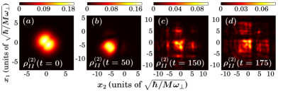
Figure 13: Instantaneous two-body reduced density matrix of the impurities at different time-instants of the evolution (see legends) following a continuous shaking of the harmonic oscillator at frequency $\displaystyle\omega_{D}=1.15$. The remaining system parameters are the same as in Fig. 8.

V.5 Two-body dynamics of the impurities

Next, we monitor the spatially resolved dynamics of the two impurities with respect to one another by resorting to the diagonal of the two-body bosonic reduced density matrix

$$\begin{split}\rho^{(2)}_{II}(x_{1},x_{2};t)=\bra{\Psi_{MB}(t)}\hat{\Psi}^{I\dagger}(x_{1})\hat{\Psi}^{I\dagger}(x_{2})\\ \times\hat{\Psi}^{I}(x_{1})\hat{\Psi}^{I}(x_{2})\ket{\Psi_{MB}(t)}.\end{split}$$ (11)

In this expression, $\displaystyle\hat{\Psi}^{I}(x_{1})$ is the corresponding bosonic field operator that annihilates a boson at position $\displaystyle x_{1}$. Recall that $\displaystyle\rho^{(2)}_{II}(x_{1},x_{2};t)$ provides the probability of measuring simultaneously one boson to be located at $\displaystyle x_{1}$ and the other one at $\displaystyle x_{2}$ Mistakidis et al. (2018a, 2019d); Naraschewski and Glauber (1999). For our investigation we focus on large driving frequencies where the impurities reside within the bosonic gas throughout the evolution [see also Figs. 8 ($\displaystyle b_{3}$), ($\displaystyle b_{4}$)] and also the interparticle correlations of the system are enhanced [Fig. 11]. Moreover since the impurities are trapped within the bosonic gas they are dressed by its excitations forming quasiparticles. Consequently, these quasiparticles can either move independently or interact thereby forming a pair Theel et al. (2019); Dehkharghani et al. (2018); Mistakidis et al. (2019g, f).

Figure 16 depicts $\displaystyle\rho^{(2)}_{II}(x_{1},x_{2};t)$ at certain time-instants of the evolution upon considering a continuous shaking of the impurities harmonic oscillator at $\displaystyle\omega_{D}=1.15$. Initially $\displaystyle t=0$ [Fig. 16 (a)] the two bosons reside together at the trap center as $\displaystyle\rho^{(2)}_{II}(-2<x_{1}<2,-2<x_{2}<2;t=0)$ exhibits a high two-body probability peak in the domain $\displaystyle-2<x_{1},x_{2}<2$. As time evolves the impurities oscillate within the bosonic bath [see also Fig. 8 ($\displaystyle b_{3}$)] as a pair since $\displaystyle\rho^{(2)}_{II}(-8<x_{1}<-2,-8<x_{2}<-2;t=50)$ is predominantly populated [Fig. 16 ($\displaystyle b$)]. Simultaneously signatures of a delocalized behavior are observed due to the small values of the off-diagonal elements of $\displaystyle\rho^{(2)}_{II}(x_{1},x_{2};t=50)$. Entering deeper in the evolution the aforementioned delocalization of the impurities becomes more prominent since $\displaystyle\rho^{(2)}_{II}(x_{1},x_{2};t)$ disperses as shown in Figs. 16 ($\displaystyle c$), ($\displaystyle d$). This dispersive behavior of $\displaystyle\rho^{(2)}_{II}(x_{1},x_{2};t)$ is inherently related to the one exhibited by $\displaystyle\rho^{(1)}_{I}(x,t)$ in Fig. 8 ($\displaystyle c$) suggesting from a two-body perspective the involvement of excited states in the impurity dynamics. Most importantly, the diagonal of $\displaystyle\rho^{(2)}_{II}(x_{1},x_{2};t)$ is predominantly populated [Figs. 16 ($\displaystyle c$), ($\displaystyle d$)] which is suggestive of the presence of attractive induced impurity-impurity interactions Theel et al. (2019); Mistakidis et al. (2019d); Dehkharghani et al. (2018); Mistakidis et al. (2019g, f). Similar pairing mechanisms of bosonic impurities mainly concentrating on the stationary properties of bosonic mixtures have been discussed in Refs. Dehkharghani et al. (2018); Camacho-Guardian et al. (2018); Klein and Fleischhauer (2005).

VI Conclusions

We have investigated the driven dynamics of two repulsively interacting impurities immersed in a bosonic bath following two different shaking protocols of the harmonic trap of the impurities. Namely, the shaking is either performed via a pulse consisting of two driving periods and then the system is left to evolve unperturbed or it is maintained throughout the evolution corresponding to a continuous driving. A particular focus has been placed on setups where the impurities and the bath are initially spatially overlapping (miscible components) while the case of initially immiscible components has also been briefly discussed. Moreover the dynamical response of the impurities has been carefully explored for a wide range of driving frequencies ranging from low to high frequency driving and has been characterized by utilizing several diagnostics including one- and two-body observables as well as the individual energy contributions of the species.

Regarding the pulse driving scenario and for initially miscible (overlapping) components we have identified different dynamical response regimes of the impurities depending on the driving frequency as compared to the frequency of the harmonic trap. For low driving frequencies, in the course of the shaking the impurities oscillate in space within and outside their host closely following the motion of their trap. However after the termination of the pulse their oscillation amplitude decays and they are trapped in the bosonic gas. Entering the resonant driving regime, i.e. for a driving frequency close to the harmonic oscillator one, the impurities undergo a more complex dynamics. Namely in the duration of the shaking they perform large amplitude irregular oscillations escaping and re-entering into the bosonic gas while afterwards they essentially decouple from the bath. For large driving frequencies, much larger than the external trap frequency, it is shown that the impurities remain predominantly trapped within the bosonic gas especially after the pulse has terminated and exhibit a dispersive behavior for long evolution times. Turning to initially immiscible components we have shown that despite the intricate tendency for zero spatial overlap, the impurities subjected to moderate drivings feature a dispersive behavior within the bosonic gas after the pulse is terminated. However a vigorous shaking renders the impurities to oscillate around the edges of the Thomas-Fermi background of the bosonic bath, thus preserving their spatial separation with the bath almost intact.

Considering a continuous shaking of the trap of the impurities for miscible components we observed that a similar overall phenomenology as for the pulse driven case takes place especially for very low and high driving frequencies. However, the dynamical response of the impurities here is periodically repeated in time due to the driving protocol and regarding the high frequency driving the impurities are found to be better trapped into their host compared to the pulse driving. Most importantly, it is showcased that in the resonantly driven regime the impurities perform a periodic oscillatory motion, moving within and escaping from the BEC background, while featuring multiple collision events with the latter. Furthermore independently of the driving frequency and the protocol the motion of the impurities perturbs the bosonic bath which is subsequently excited performing a collective dipole motion. Also these excitations are more prominent for high frequency drivings where the impurities mostly reside within their host.

Examining the individual energy contributions of each species we reveal that when the impurities are trapped into the bosonic bath they transfer energy to the latter, a behavior that is more pronounced for large driving frequencies. We expose the participation of inter- and intraspecies correlations during the dynamics and show that their degree is enhanced for high driving frequencies. The development of coherence losses both in the bosonic gas and the impurities is unveiled and most importantly it is found that the impurities predominantly move as a pair and not individually.

There are several promising research directions, based on the present work, to be considered in future endeavors. A straightforward one is to employ two fermionic impurities immersed either in a bosonic or a fermionic environment and investigate the emergent periodically driven dynamics induced by the protocol used herein. Another interesting perspective is to construct in the continuous low frequency driving case an effective model according to which the impurities are dressed by the excitations of the BEC when they lie inside the latter but they are undressed during the time-intervals that they reside outside their host. Within such a model it might be possible to identify the corresponding polaronic properties of the impurities such as their effective mass and induced interactions Mistakidis et al. (2019f, b). Moreover, the driven dynamics of impurities trapped in an optical lattice Keiler and Schmelcher (2018) instead of a harmonic trap in order to control their transport properties is an interesting perspective. Finally, in the framework of the present work, the simulation of the corresponding contrast by considering spinor impurities in order to identify possibly emerging polaronic states Mistakidis et al. (2019a) is definitely worth pursuing.

Appendix A Periodically driven dynamics of a mass-imbalanced mixture

In the main text, all of the presented results have been focusing on mass balanced mixtures. Another interesting scenario is to consider a mass-imbalanced system and in particular the case of heavy impurities immersed in the bosonic bath in order to inspect whether the mass-imbalance can potentially alter the nonequilibrium dynamics discussed in Sec. V. Such a typical mass-imbalance bosonic mixture corresponds to a ⁸⁷Rb bath and two ¹³³Cs impurities prepared at the hyperfine states $\displaystyle\Ket{F=1,m_{F}=0}$ and $\displaystyle\Ket{F=3,m_{F}=2}$ respectively and trapped in the same harmonic oscillator Hohmann et al. (2015).

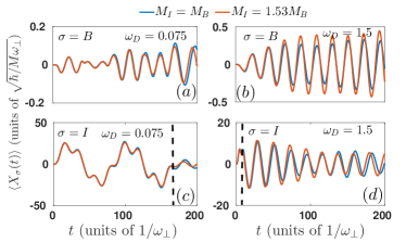
Figure 14: Comparison of the temporal-evolution of the center-of-mass of the bosonic bath $\displaystyle\langle X_{B}(t)\rangle$ (upper panels) and the impurities $\displaystyle\langle X_{I}(t)\rangle$ (lower panels) between a mass-balanced and a mass-imbalanced mixture (see legend) at different driving frequencies $\displaystyle\omega_{D}$ (see legend). The pulse shaking of the harmonic trap of the impurities is performed for two driving periods until $\displaystyle t=t_{f}=4\pi/\omega_{D}$ (see the vertical lines) and afterwards the system is left to evolve unperturbed. The remaining system parameters are the same as in Fig. 1.

The time-evolution of the center-of-mass oscillation of the impurities $\displaystyle\langle X_{I}(t)\rangle$ and the bosonic gas $\displaystyle\langle X_{B}(t)\rangle$, following a pulse shaking of the harmonic trap of the impurities, is shown in Fig. 14 for selective driving frequencies and for both a mass-balanced and a mass-imbalanced mixture. Overall, we observe that the dynamical response of both the bosonic gas and the impurities is not significantly affected by the mass-imbalance. More specifically, for low driving frequencies $\displaystyle\omega_{D}=0.075$ both $\displaystyle\langle X_{B}(t)\rangle$ [Fig. 14 (a)] and $\displaystyle\langle X_{I}(t)\rangle$ [Fig. 14 (c)] are seen to be essentially insensitive to the considered mass ratio. A similar behavior is encountered for high driving frequencies e.g. $\displaystyle\omega_{D}=1.5$ but here the oscillation amplitude of $\displaystyle\langle X_{B}(t)\rangle$ is slightly larger in the mass-imbalanced case [Fig. 14 (b)]. This is an expected behavior because the heavy impurities can perturb their host to a larger extent compared to the lighter ones due to $\displaystyle m_{Cs}>m_{Rb}$. Moreover, tiny deviations occur also in the oscillation amplitude of $\displaystyle\langle X_{I}(t)\rangle$ [Fig. 14 (d)] between the mass balanced and imbalanced cases but with no major tendency.

Appendix B Remarks on the many-body computational methodology

As we discussed in Sec. II.2, in order to study the periodically driven nonequilibrium dynamics of the bosonic mixture, we rely on the multi-layer multi-configurational time-dependent Hartree method for atomic mixtures (ML-MCTDHX) Cao et al. (2017, 2013); Krönke et al. (2013). It is an ab-initio approach for solving the time-dependent Schrödinger equation of multicomponent systems with bosonic Mistakidis et al. (2018a); Katsimiga et al. (2017a, b, 2018) or fermionic  Koutentakis et al. (2019); Siegl et al. (2018) constituents including also spin degrees of freedom Mistakidis et al. (2019c); Koutentakis et al. (2019). The main facet of this numerical approach is that the many-body wavefunction is expanded with respect to a time-dependent and variationally optimized basis. The latter enables us to span the relevant subspace of the Hilbert space at each time-instant of the dynamics in a more efficient manner when compared to methods employing a time-independent basis. Furthermore, its multi-layer ansatz for the total wavefunction is tailored to capture both the intra- and interspecies correlations emerging during the nonequilibrium dynamics of a multicomponent system.

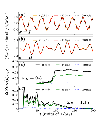
Figure 15: Time-evolution of the center-of-mass of ($\displaystyle a$) the two interacting impurities $\displaystyle\langle X_{I}(t)\rangle$ and ($\displaystyle b$) the bosonic gas $\displaystyle\langle X_{B}(t)\rangle$ for different orbital configurations ($\displaystyle D;d_{B};d_{I}$) (see legend) at a high driving frequency $\displaystyle\omega_{D}=1.5$. Dynamics of the deviation of the von-Neumann entropy between the $\displaystyle C=(10;3;6)$ and other orbital combinations ($\displaystyle D;d_{B};d_{I}$) (see legend) for driving frequency ($\displaystyle c$) $\displaystyle\omega_{D}=0.3$ and ($\displaystyle d$) $\displaystyle\omega_{D}=1.15$. The shaking of the harmonic oscillator of the impurities is performed throughout the evolution. The mixture consists of $\displaystyle N_{B}=100$ bosons with $\displaystyle g_{BB}=0.5$ and $\displaystyle N_{I}=2$ interacting $\displaystyle g_{II}=0.4$ impurities in a harmonic trap of frequency $\displaystyle\omega=0.3$. The interspecies repulsion is $\displaystyle g_{BI}=0.2$ and the mixture is prepared in its ground state.

Within this methodology, the underlying Hilbert space truncation is designated by the used orbital configuration space $\displaystyle C=(D;d_{B};d_{I})$. In this notation, $\displaystyle D$ and $\displaystyle d_{B}$, $\displaystyle d_{I}$ refer to the number of species functions [Eq. (3)] and single-particle functions [Eq. (4)] of each species. For our numerical simulations, a primitive basis corresponding to a sine discrete variable representation involving 500 grid points is employed. Note also that this sine discrete variable representation intrinsically introduces hard-wall boundary conditions which are imposed herein at $\displaystyle x_{\pm}=\pm 50$. Their location do not affect the presented results since there are no appreciable densities beyond $\displaystyle x_{\pm}=\pm 25$. To infer the convergence of the many-body simulations we systematically vary the numerical configuration space $\displaystyle C=(D;d_{B};d_{I})$ and ensure that all observables of interest become up to a certain level of accuracy insensitive. We remark that all many-body simulations discussed in the main text have been performed using $\displaystyle C=(10;3;6)$.

To showcase the numerical convergence we exemplarily demonstrate the behavior of the center-of-mass motion of the impurities $\displaystyle\langle X_{I}(t)\rangle$ and of the bosonic bath $\displaystyle\langle X_{B}(t)\rangle$ following a continuous periodic driving at $\displaystyle\omega_{D}=1.5$ for distinct orbital configurations $\displaystyle C^{\prime}=(D^{\prime};d^{\prime}_{B};d^{\prime}_{I})$ in Fig. 15. Recall that at such high driving frequencies the degree of correlations inherent in the system is maximized [Fig. 11]. Inspecting Fig. 15, it can readily seen that both $\displaystyle\langle X_{I}(t)\rangle$ [Fig. 15 ($\displaystyle a$)] and $\displaystyle\langle X_{B}(t)\rangle$ [Fig. 15 ($\displaystyle b$)] are adequately converged since they are insensitive to the variation of the orbital configuration space $\displaystyle C=(D;d_{B};d_{I})$. For instance, the maximum deviation of $\displaystyle\langle X_{I}(t)\rangle$ [$\displaystyle\langle X_{B}(t)\rangle$] between the $\displaystyle C=(10;3;6)$ and $\displaystyle C^{\prime}=(10;3;4)$ in the course of the time-evolution is at most $\displaystyle 0.2\%$ [$\displaystyle 0.1\%$].

Moreover, we present the numerical convergence of the von-Neumann entropy during the dynamics for a continuous driving characterized by $\displaystyle\omega_{D}=0.3$ (resonant driving) and $\displaystyle\omega_{D}=1.15$ (fast driving). Note here that for $\displaystyle\omega_{D}=1.15$ the von-Neumann entropy becomes maximal, see also Fig. 11 (a). To this end, we illustrate the relative difference of $\displaystyle S_{VN}(t)$ calculated within the $\displaystyle C=(10;3;6)$ and different orbital configurations $\displaystyle C^{\prime}=(D^{\prime};d_{B}^{\prime};d_{I}^{\prime})$ i.e.

$$\Delta S_{VN}(t)_{C,C^{\prime}}=\frac{\left|S_{VN}(t)_{C}-S_{VN}(t)_{C^{\prime}}\right|}{S_{VN}(t)_{C}}.$$ (12)

The time-evolution of $\displaystyle\Delta S_{VN}(t)_{C,C^{\prime}}$ is shown in Fig. 15 at resonant driving frequencies $\displaystyle\omega_{D}=0.3$ [Fig. 15 (c)] and fast drivings with $\displaystyle\omega_{D}=1.15$ [Fig. 15 (d)] for a variety of orbital configurations $\displaystyle C^{\prime}$ and fixed $\displaystyle C=(10;3;6)$. Inspecting $\displaystyle\Delta S_{VN}(t)_{C,C^{\prime}}$ we deduce that $\displaystyle S_{VN}(t)$ is converged at both $\displaystyle\omega_{D}=0.3$ and $\displaystyle\omega_{D}=1.15$. For instance at $\displaystyle\omega_{D}=0.3$ the deviation of $\displaystyle\Delta S_{VN}(t)_{C,C^{\prime}}$ with $\displaystyle C=(10;3;6)$ and $\displaystyle C^{\prime}=(10;2;6)$ [$\displaystyle C=(8;2;6)$] is smaller than $\displaystyle 1\%$ [$\displaystyle 4\%$] throughout the evolution [Fig. 15 (c)]. Turning to $\displaystyle\omega_{D}=1.15$ [Fig. 7 (d)], we observe that $\displaystyle\Delta S_{VN}(t)_{C,C^{\prime}}$ between the orbital configurations $\displaystyle C=(10;3;6)$ and $\displaystyle C^{\prime}=(10;2;6)$ [$\displaystyle C^{\prime}=(8;2;6)$] acquires a maximum value of the order of $\displaystyle 1\%$ [$\displaystyle 5\%$] in the course of the time-evolution. Additionally, let us comment that the same analysis has been done for all other observables and driving frequencies discussed in the main text and found to be sufficiently converged as well (results not shown here for brevity).

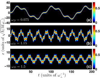
Figure 16: Time-evolution of the single-particle density of two bosons trapped in a continuously shaken harmonic oscillator potential for specific driving frequencies $\displaystyle\omega_{D}$ (see legends). The system consists of $\displaystyle N=2$ repulsively interacting bosons with $\displaystyle g=0.4$. It is trapped in a harmonic oscillator with frequency $\displaystyle\omega=0.3$ and it is initialized into its ground state.

Appendix C Shaking dynamics of two-bosons

To expose the effects caused by the presence of the bosonic bath on the dynamical response of the impurities described in the main text, we briefly discuss the dynamics of two bosons trapped in a continuously shaken harmonic trap. In particular, we consider two ($\displaystyle N=2$) repulsively interacting bosons in a harmonic trap of frequency $\displaystyle\omega=0.3$. The system is initialized into its ground state with interparticle interaction strength $\displaystyle g=0.4$. To induce the dynamics the harmonic trap is periodically shaken throughout the time-evolution and the system obeys the following Hamiltonian

$$\begin{split}&H=\sum_{i=1}^{N}-\frac{\hbar^{2}}{2M}\bigg{(}\frac{\partial}{\partial x_{i}}\bigg{)}^{2}+\sum_{i=1}^{N}\frac{1}{2}M\omega^{2}x_{i}^{2}\\ &+\frac{1}{2}M\omega^{2}\sum_{i=1}^{N}\big{(}x_{i}-\mathcal{A}\sin(\omega_{D}t)\big{)}^{2}+g\sum_{i\geq j}\delta(x_{i}-x_{j}).\end{split}$$ (13)

In this expression, $\displaystyle\mathcal{A}$ and $\displaystyle\omega_{D}$ refer to the amplitude and the frequency of the driving respectively. To perform a direct comparison with the observations made in Section V we use $\displaystyle\mathcal{A}=20$ and study the dynamics for different driving frequencies $\displaystyle\omega_{D}$ while keeping fixed all other parameters of the system.

The resulting time-evolution of the two boson single-particle density, $\displaystyle\rho^{(1)}(x;t)$ is illustrated in Fig. 16 for different driving frequencies. As it can be seen in Fig. 16 (a), for small driving frequencies such as $\displaystyle\omega_{D}=0.075$ the two bosons follow their driven potential and undergo an overall oscillatory motion. At the initial evolution times $\displaystyle\rho^{(1)}(x;t)$ moves to the $\displaystyle x>0$ direction reaching $\displaystyle(x\approx 27)\gg(\mathcal{A}=20)$ at $\displaystyle t\approx 16$ and then turns towards $\displaystyle x<0$ due to the presence of the trap while featuring a backward motion around $\displaystyle t\approx 27$. Subsequently $\displaystyle\rho^{(1)}(x;t)$ moves to the $\displaystyle x<0$ direction performing a similar to the above-mentioned backward and forward motion until it arrives at $\displaystyle x\approx-27$ where it again turns its motion to the trap center. In this way, the first oscillation period of the driving is completed and afterwards a similar to the above-described motion occurs within each driving cycle [Figs. 16 (a)]. Note that for these weak driving frequencies the two-boson dynamical response is similar to the one of the two impurities immersed in a BEC background, compare Fig. 8 ($\displaystyle b_{1}$) and Fig. 16 (a). A notable difference occurring in the response of the aforementioned setups is that the shape of the single-particle density of the two impurities changes in the course of the time-evolution due to their collisions with the BEC medium, see e.g. Fig. 8 ($\displaystyle b_{1}$) at $\displaystyle t\approx 34$, an event that is absent in the dynamics of the two bosons. We remark that a similar overall phenomenology regarding the shaken dynamics of two impurities inside a BEC and the two bosons takes place also for driving frequencies $\displaystyle\omega_{D}<0.6$.

However, entering the driving regime with $\displaystyle\omega_{D}>0.5$ significant alterations between the responses of these setups occur. To exemplify these differences we showcase $\displaystyle\rho^{(1)}(x;t)$ of two bosons for $\displaystyle\omega_{D}=1.15$ and $\displaystyle\omega_{D}=1.5$ in Figs. 16 (b) and (c) respectively. Indeed, in both cases $\displaystyle\rho^{(1)}(x;t)$ performs a multifrequency oscillatory behavior of constant amplitude. This is in sharp contrast to the time-evolution of two impurities shown in Figs. 8 ($\displaystyle b_{3}$), ($\displaystyle b_{4}$) where $\displaystyle\rho^{(1)}_{I}(x;t)$ exhibits a decaying amplitude oscillatory motion within the bosonic bath throughout the dynamics. Also, $\displaystyle\rho^{(1)}_{I}(x;t)$ due to impurity-BEC interactions shows a spatially delocalized behavior for $\displaystyle t>100$ [Fig. 8 ($\displaystyle b_{3}$), ($\displaystyle b_{4}$)] whilst $\displaystyle\rho^{(1)}(x;t)$ exhibits a localized shape throughout the evolution [Fig. 16 ($\displaystyle b$), ($\displaystyle d$)]. Summarizing, we deduce that for $\displaystyle\omega_{D}>0.6$ the dynamical response of two shaken bosonic impurities is very different from the one of two bosons. This behavior can be explained by the fact that for a fast shaking ($\displaystyle\omega_{D}>0.6$) of the harmonic trap the impurities motion is mainly restricted within their host and therefore impurity-BEC interaction effects dominate the dynamics.

References

- Will et al. (2011) S. Will, T. Best, S. Braun, U. Schneider, and I. Bloch, Phys. Rev. Lett. 106, 115305 (2011).
- Massignan et al. (2014) P. Massignan, M. Zaccanti, and G. M. Bruun, Rep. Progr. Phys. 77, 034401 (2014).
- Palzer et al. (2009) S. Palzer, C. Zipkes, C. Sias, and M. Köhl, Phys. Rev. Lett. 103, 150601 (2009).
- Modugno et al. (2002) G. Modugno, M. Modugno, F. Riboli, G. Roati, and M. Inguscio, Phys. Rev. Lett. 89, 190404 (2002).
- Burchianti et al. (2018) A. Burchianti, C. D’Errico, S. Rosi, A. Simoni, M. Modugno, C. Fort, and F. Minardi, Phys. Rev. A 98, 063616 (2018).
- Landau (1933) L. D. Landau, Phys. Z. Sowjetunion 3, 644 (1933).
- Fröhlich (1954) H. Fröhlich, Advances in Physics 3, 325 (1954).
- Schmidt et al. (2018) R. Schmidt, M. Knap, D. A. Ivanov, J.-S. You, M. Cetina, and E. Demler, Rep. Progr. Phys. 81, 024401 (2018).
- Khandekar et al. (1988) D. C. Khandekar, K. V. Bhagwat, and S. V. Lawande, Phys. Rev. B 37, 3085 (1988).
- Feynman et al. (1962) R. P. Feynman, R. W. Hellwarth, C. K. Iddings, and P. M. Platzman, Phys. Rev. 127, 1004 (1962).
- Kadanoff (1963) L. P. Kadanoff, Phys. Rev. 130, 1364 (1963).
- Casteels et al. (2013) W. Casteels, J. Tempere, and J. T. Devreese, Phys. Rev. A 88, 013613 (2013).
- Camacho-Guardian et al. (2018) A. Camacho-Guardian, L. A. Peña Ardila, T. Pohl, and G. M. Bruun, Phys. Rev. Lett. 121, 013401 (2018).
- Chin et al. (2010) C. Chin, R. Grimm, P. Julienne, and E. Tiesinga, Rev. Mod. Phys. 82, 1225 (2010).
- Köhler et al. (2006) T. Köhler, K. Góral, and P. S. Julienne, Rev. Mod. Phys. 78, 1311 (2006).
- Jørgensen et al. (2016) N. B. Jørgensen, L. Wacker, K. T. Skalmstang, M. M. Parish, J. Levinsen, R. S. Christensen, G. M. Bruun, and J. J. Arlt, Phys. Rev. Lett. 117, 055302 (2016).
- Hu et al. (2016) M.-G. Hu, M. J. Van de Graaff, D. Kedar, J. P. Corson, E. A. Cornell, and D. S. Jin, Phys. Rev. Lett. 117, 055301 (2016).
- Catani et al. (2009) J. Catani, G. Barontini, G. Lamporesi, F. Rabatti, G. Thalhammer, F. Minardi, S. Stringari, and M. Inguscio, Phys. Rev. Lett. 103, 140401 (2009).
- Fukuhara et al. (2013) T. Fukuhara, A. Kantian, M. Endres, M. Cheneau, P. Schauß, S. Hild, D. Bellem, U. Schollwöck, T. Giamarchi, C. Gross, I. Bloch, and S. Kuhr, Nat. Phys. 9, 235 (2013).
- Scazza et al. (2017) F. Scazza, G. Valtolina, P. Massignan, A. Recati, A. Amico, A. Burchianti, C. Fort, M. Inguscio, M. Zaccanti, and G. Roati, Phys. Rev. Lett. 118, 083602 (2017).
- Koschorreck et al. (2012) M. Koschorreck, D. Pertot, E. Vogt, B. Fröhlich, M. Feld, and M. Köhl, Nature 485, 615 (2012).
- Kohstall et al. (2012) C. Kohstall, M. Zaccanti, M. Jag, A. Trenkwalder, P. Massignan, G. M. Bruun, F. Schreck, and R. Grimm, Nature 485, 615 (2012).
- Cetina et al. (2015) M. Cetina, M. Jag, R. S. Lous, J. T. Walraven, R. Grimm, R. S. Christensen, and G. M. Bruun, Phys. Rev. Lett. 115, 135302 (2015).
- Cetina et al. (2016) M. Cetina, M. Jag, R. S. Lous, I. Fritsche, J. T. Walraven, R. Grimm, J. Levinsen, M. M. Parish, R. Schmidt, M. Knap, and E. Demler, Science 354, 96 (2016).
- Koepsell et al. (2019) J. Koepsell, J. Vijayan, P. Sompet, F. Grusdt, T. A. Hilker, E. Demler, G. Salomon, I. Bloch, and C. Gross, Nature , 1 (2019).
- Grusdt and Demler (2015) F. Grusdt and E. Demler, Quantum Matter at Ultralow Temperatures 191, 325 (2015).
- Bruderer et al. (2007) M. Bruderer, A. Klein, S. R. Clark, and D. Jaksch, Phys. Rev. A 76, 011605 (2007).
- Casteels et al. (2012) W. Casteels, J. Tempere, and J. T. Devreese, Phys. Rev. A 86, 043614 (2012).
- Kain and Ling (2016) B. Kain and H. Y. Ling, Phys. Rev. A 94, 013621 (2016).
- Volosniev and Hammer (2017) A. G. Volosniev and H.-W. Hammer, Phys. Rev. A 96, 031601 (2017).
- Dehkharghani et al. (2018) A. S. Dehkharghani, A. G. Volosniev, and N. T. Zinner, Phys. Rev. Lett. 121, 080405 (2018).
- Mistakidis et al. (2019a) S. I. Mistakidis, G. C. Katsimiga, G. M. Koutentakis, and P. Schmelcher, New J. Phys. 21, 043032 (2019a).
- Ardila and Pohl (2018) L. A. P. Ardila and T. Pohl, J. Phys. B: At. Mol. and Opt. Phys. 52, 015004 (2018).
- Ardila and Giorgini (2015) L. A. P. Ardila and S. Giorgini, Phys. Rev. A 92, 033612 (2015).
- Ardila et al. (2019) L. A. P. Ardila, N. B. Jørgensen, T. Pohl, S. Giorgini, G. Bruun, and J. Arlt, Phys. Rev. A 99, 063607 (2019).
- Grusdt et al. (2018) F. Grusdt, K. Seetharam, Y. Shchadilova, and E. Demler, Phys. Rev. A 97, 033612 (2018).
- Grusdt et al. (2017a) F. Grusdt, R. Schmidt, Y. E. Shchadilova, and E. Demler, Phys. Rev. A 96, 013607 (2017a).
- Tempere et al. (2009) J. Tempere, W. Casteels, M. K. Oberthaler, S. Knoop, E. Timmermans, and J. T. Devreese, Phys. Rev. B 80, 184504 (2009).
- Panochko and Pastukhov (2019) G. Panochko and V. Pastukhov, arXiv:1909.01256 (2019).
- Mistakidis et al. (2019b) S. I. Mistakidis, A. G. Volosniev, N. T. Zinner, and P. Schmelcher, Phys. Rev. A 100, 013619 (2019b).
- Mistakidis et al. (2019c) S. I. Mistakidis, G. C. Katsimiga, G. M. Koutentakis, T. Busch, and P. Schmelcher, Phys. Rev. Lett. 122, 183001 (2019c).
- Volosniev et al. (2015) A. G. Volosniev, H.-W. Hammer, and N. T. Zinner, Phys. Rev. A 92, 023623 (2015).
- Mistakidis et al. (2019d) S. I. Mistakidis, L. Hilbig, and P. Schmelcher, Phys. Rev. A 100, 023620 (2019d).
- Shchadilova et al. (2016) Y. E. Shchadilova, R. Schmidt, F. Grusdt, and E. Demler, Phys. Rev. Lett. 117, 113002 (2016).
- Kamar et al. (2019) N. A. Kamar, A. Kantian, and T. Giamarchi, Phys. Rev. A 100, 023614 (2019).
- Boyanovsky et al. (2019) D. Boyanovsky, D. Jasnow, X.-L. Wu, and R. C. Coalson, Phys. Rev. A 100, 043617 (2019).
- Grusdt et al. (2017b) F. Grusdt, G. E. Astrakharchik, and E. Demler, New J. Phys. 19, 103035 (2017b).
- Guebli and Boudjemâa (2019) N. Guebli and A. Boudjemâa, J. Phys. B: At. Mol. and Opt. Phys. 52, 185303 (2019).
- Knap et al. (2012) M. Knap, A. Shashi, Y. Nishida, A. Imambekov, D. A. Abanin, and E. Demler, Phys. Rev. X 2, 041020 (2012).
- Anderson (1967) P. W. Anderson, Phys. Rev. Lett. 18, 1049 (1967).
- Mistakidis et al. (2019e) S. I. Mistakidis, F. Grusdt, G. M. Koutentakis, and P. Schmelcher, New J. Phys. 21, 103026 (2019e).
- Lausch et al. (2018) T. Lausch, A. Widera, and M. Fleischhauer, Phys. Rev. A 97, 023621 (2018).
- Cai et al. (2010) Z. Cai, L. Wang, X. Xie, and Y. Wang, Phys. Rev. A 81, 043602 (2010).
- Johnson et al. (2011) T. H. Johnson, S. R. Clark, M. Bruderer, and D. Jaksch, Phys. Rev. A 84, 023617 (2011).
- Siegl et al. (2018) P. Siegl, S. I. Mistakidis, and P. Schmelcher, Phys. Rev. A 97, 053626 (2018).
- Theel et al. (2019) F. Theel, K. Keiler, S. I. Mistakidis, and P. Schmelcher, arXiv:1909.00998 (2019).
- Burovski et al. (2014) E. Burovski, V. Cheianov, O. Gamayun, and O. Lychkovskiy, Phys. Rev. A 89, 041601 (2014).
- Lychkovskiy et al. (2018) O. Lychkovskiy, O. Gamayun, and V. Cheianov, Phys. Rev. B 98, 024307 (2018).
- Meinert et al. (2017) F. Meinert, M. Knap, E. Kirilov, K. Jag-Lauber, M. B. Zvonarev, E. Demler, and H.-C. Nägerl, Science 356, 945 (2017).
- Knap et al. (2014) M. Knap, C. J. Mathy, M. Ganahl, M. B. Zvonarev, and E. Demler, Phys. Rev. Lett. 112, 015302 (2014).
- Gamayun et al. (2018) O. Gamayun, O. Lychkovskiy, E. Burovski, M. Malcomson, V. V. Cheianov, and M. B. Zvonarev, Phys. Rev. Lett. 120, 220605 (2018).
- Li and Kuang (2019) Z. Li and L.-M. Kuang, arXiv:1909.03374 (2019).
- Yoshida et al. (2018) S. M. Yoshida, S. Endo, J. Levinsen, and M. M. Parish, Phys. Rev. X 8, 011024 (2018).
- Blume (2019) D. Blume, Phys. Rev. A 99, 013613 (2019).
- Goldman and Dalibard (2014) N. Goldman and J. Dalibard, Phys. Rev. X 4, 031027 (2014).
- Goldman et al. (2015) N. Goldman, J. Dalibard, M. Aidelsburger, and N. R. Cooper, Phys. Rev. A 91, 033632 (2015).
- Morsch and Oberthaler (2006) O. Morsch and M. Oberthaler, Rev. Mod. Phys. 78, 179 (2006).
- Mistakidis et al. (2015) S. I. Mistakidis, T. Wulf, A. Negretti, and P. Schmelcher, J. Phys. B: At. Mol. and Opt. Phys. 48, 244004 (2015).
- Mistakidis and Schmelcher (2017) S. I. Mistakidis and P. Schmelcher, Phys. Rev. A 95, 013625 (2017).
- Mistakidis et al. (2019f) S. I. Mistakidis, A. G. Volosniev, and P. Schmelcher, arXiv:1911.05353 (2019f).
- Mistakidis et al. (2018a) S. I. Mistakidis, G. C. Katsimiga, P. G. Kevrekidis, and P. Schmelcher, New J. Phys. 20, 043052 (2018a).
- Erdmann et al. (2019) J. Erdmann, S. I. Mistakidis, and P. Schmelcher, Phys. Rev. A 99, 013605 (2019).
- Ao and Chui (1998) P. Ao and S. T. Chui, Phys. Rev. A 58, 4836 (1998).
- Nielsen et al. (2019) K. K. Nielsen, L. A. P. Ardila, G. M. Bruun, and T. Pohl, New J. Phys. 21, 043014 (2019).
- Lampo et al. (2017) A. Lampo, S. H. Lim, M. Á. García-March, and M. Lewenstein, Quantum 1, 30 (2017).
- Cao et al. (2017) L. Cao, V. Bolsinger, S. I. Mistakidis, G. M. Koutentakis, S. Krönke, J. Schurer, and P. Schmelcher, J. Chem. Phys. 147, 044106 (2017).
- Cao et al. (2013) L. Cao, S. Krönke, O. Vendrell, and P. Schmelcher, J. Chem. Phys. 139, 134103 (2013).
- Krönke et al. (2013) S. Krönke, L. Cao, O. Vendrell, and P. Schmelcher, New J. Phys. 15, 063018 (2013).
- Mistakidis et al. (2019g) S. I. Mistakidis, G. M. Koutentakis, G. C. Katsimiga, T. Busch, and P. Schmelcher, arXiv:1911.02011 (2019g).
- Egorov et al. (2013) M. Egorov, B. Opanchuk, P. Drummond, B. Hall, P. Hannaford, and A. I. Sidorov, Phys. Rev. A 87, 053614 (2013).
- Parker et al. (2013) C. V. Parker, L.-C. Ha, and C. Chin, Nature Physics 9, 769 (2013).
- Olshanii (1998) M. Olshanii, Phys. Rev. Lett. 81, 938 (1998).
- Horodecki et al. (2009) R. Horodecki, P. Horodecki, M. Horodecki, and K. Horodecki, Rev. Mod. Phys. 81, 865 (2009).
- Roncaglia et al. (2014) M. Roncaglia, A. Montorsi, and M. Genovese, Phys. Rev. A 90, 062303 (2014).
- Köhler et al. (2019) F. Köhler, K. Keiler, S. I. Mistakidis, H.-D. Meyer, and P. Schmelcher, J. Chem. Phys. 151, 054108 (2019).
- Frenkel (1934) J. Frenkel, Claredon Press, Oxford, 1934 , 423 (1934).
- Dirac (1930) P. A. Dirac, Proc. Camb. Phil. Soc. 26, 376 (1930).
- Naraschewski and Glauber (1999) M. Naraschewski and R. J. Glauber, Phys. Rev. A 59, 4595 (1999).
- Sakmann et al. (2008) K. Sakmann, A. I. Streltsov, O. E. Alon, and L. S. Cederbaum, Phys. Rev. A 78, 023615 (2008).
- Kevrekidis et al. (2007) P. G. Kevrekidis, D. J. Frantzeskakis, and R. Carretero-González, Emergent nonlinear phenomena in Bose-Einstein condensates: theory and experiment, Vol. 45 (Springer Science & Business Media, 2007).
- Katsimiga et al. (2017a) G. C. Katsimiga, S. I. Mistakidis, G. M. Koutentakis, P. G. Kevrekidis, and P. Schmelcher, New J. Phys. 19, 123012 (2017a).
- Katsimiga et al. (2018) G. C. Katsimiga, S. I. Mistakidis, G. M. Koutentakis, P. G. Kevrekidis, and P. Schmelcher, Phys. Rev. A 98, 013632 (2018).
- Katsimiga et al. (2017b) G. C. Katsimiga, S. I. Mistakidis, G. M. Koutentakis, P. G. Kevrekidis, and P. Schmelcher, New J. Phys. 19, 123012 (2017b).
- Mistakidis et al. (2018b) S. I. Mistakidis, G. C. Katsimiga, P. G. Kevrekidis, and P. Schmelcher, New J. Phys. 20, 043052 (2018b).
- Timmermans (1998) E. Timmermans, Phys. Rev. Lett. 81, 5718 (1998).
- Klein and Fleischhauer (2005) A. Klein and M. Fleischhauer, Phys. Rev. A 71, 033605 (2005).
- Keiler and Schmelcher (2018) K. Keiler and P. Schmelcher, New J. Phys. 20, 103042 (2018).
- Hohmann et al. (2015) M. Hohmann, F. Kindermann, B. Gänger, T. Lausch, D. Mayer, F. Schmidt, and A. Widera, EPJ Quantum Technology 2, 23 (2015).
- Koutentakis et al. (2019) G. M. Koutentakis, S. I. Mistakidis, and P. Schmelcher, New J. Phys. 21, 053005 (2019).