Abstract
The increasing interest in the phenomenology of the Standard Model Effective Field Theory (SMEFT), has led to the development of a wide spectrum of public codes which implement automatically different aspects of the SMEFT for phenomenological applications. In order to discuss the present and future of such efforts, the “SMEFT-Tools 2019” Workshop was held at the IPPP Durham on the 12th-14th June 2019. Here we collect and summarize the contents of this workshop.

1 Introduction

Testing the Standard Model (SM) and searching for New Physics (NP) are among the main priorities in High-Energy Physics. Whether or not new particles are directly produced at the LHC, indirect searches will remain crucially important to test the SM and to characterize possible NP patterns. Indirect searches, defined as searches for far-off-shell effects from new degrees of freedom, are best framed in the context of Effective Field Theories (EFTs). Constraints from direct searches indicate that these new degrees of freedom, if present, appear at scales much above the Electroweak (EW) scale. Therefore, the relevant EFT for the study of beyond-the-SM (BSM) physics at the EW scale is the Standard Model Effective Field Theory (SMEFT) [1, 2]. For observables at lower energies, such as hadron and lepton decays, other EFTs must be constructed where particles with weak-scale masses have been integrated out [3, 4, 5]. The EFT below the EW scale has been called the Weak Effective Theory (WET) or the Low Energy EFT (LEFT).

Thus, the bulk of any phenomenological analysis of heavy BSM physics at low energies involves a series of steps of matching and renormalization-group evolution, followed by the calculation of low-energy observables. Since such a procedure is tedious in practice, considerable effort is being devoted to developing public software designed to perform these tasks in an automatic and generic manner. Some of the available codes are:

• Construction of EFT Bases: DEFT [6], BasisGen [7], abc-eft [8] .

• Feynman Rules for the SMEFT: SmeftFR [9].

• Matching calculators: MatchingTools [10], Matchmaker [11], CoDEx [12]

• Generic Matching+Running codes: DsixTools [13], wilson [14].

• Fitters: SMEFiT [15], smelli [16].

• Observables and Montecarlo enablers: EOS [17], flavio [18], SMEFTsim [19].

In this context, the 1st Workshop on Tools for Low-Energy SMEFT Phenomenology, SMEFT-Tools 2019:

https://indico.cern.ch/event/787665/

was held at IPPP Durham from 12-14th June 2019 with the purpose of discussing the status and future prospects of computing tools designed for phenomenological analyses of the SMEFT and the WET/LEFT. This report summarizes the contents of the workshop, complementing the slides available on the web. We believe that collecting brief descriptions of most of the currently available tools in this single document is going to be useful for the community.

2 BasisGen: counting EFT operators

Speaker: Juan Carlos Criado
University of Granada

BasisGen is a Python package that generates bases of operators for EFTs. An EFT is specified by giving its symmetries and field content. The package takes this information and produces a list of all possible forms for the invariant operators in the theory, together with the number independent operators of each form. It uses well-known methods in representation theory [20], based on roots and weights, which allow for general and fast calculations. To deal with integration by parts redundancy, an adaptation of the method in ref. [24] is used.

BasisGen works with any internal symmetry group of the form $G\times U(1)^{N}$, where $G$ is a semisimple Lie group. For simplicity, it assumes 4-dimensional Lorentz invariance. The fields can be in any irreducible representation of both the internal symmetry group and the Lorentz group. BasisGen generates complete sets of independent operators, taking into account group-theory identities and integration by parts. Optionally, redundancies arising from field redefinitions [25, 26, 27] can be eliminated. For the purpose of generating a basis, this is the same as using the equations of motion to remove operators [28, 29, 30].

A module containing the definition of the SMEFT is included in the package. It can be used to obtain bases of this theory with operators of arbitrary maximum dimension, but also as a starting point for defining new theories with extra fields or symmetries. Generating a dimension-6 basis takes only a few seconds in a modern laptop.

Other features of BasisGen include:

• An interface to its representation-theory functionalities, allowing the user to obtain the weight system of any irreducible representation, compute tensor products, and decompose reducible representations.

• The possibility of generating all (not necessarily invariant) operators, decomposing their representations into irreducible ones. This gives all the possible representations of new fields that couple linearly to the fields in the EFT. Such new fields are often the most relevant for phenomenology [31].

A description of the implementation and interface of BasisGen can be found in ref. [7]. Its code can be downloaded from the GitHub repository https://github.com/jccriado/basisgen. It requires Python version 3.5 or higher. It can be installed using pip by running:

⬇

> pip install basisgen

As an example of use, we consider here an EFT with symmetry group $SU(2)\times U(1)$, whose field content consists of a complex scalar doublet $\phi$ with hypercharge $1/2$. To import the necessary parts of the package, once it is installed, one can do

⬇

from basisgen import Field, EFT, scalar, irrep, algebra

The EFT is defined by

⬇

phi = Field(

name=’phi’,

lorentz_irrep=scalar,

internal_irrep=irrep(’SU2’, ’1’),

charges=[1/2]

)

my_eft = EFT(algebra(’SU2’), [phi, phi.conjugate])

Now, the following code can be used to compute a basis of operators with maximum dimension 8:

⬇

invariants = my_eft.invariants(max_dimension=8)

print(invariants)

print(”Total:”, invariants.count())

The output is:

⬇

phi phi*: 1

(phi)^2 (phi*)^2: 1

(phi)^2 (phi*)^2 D^2: 2

(phi)^2 (phi*)^2 D^4: 3

(phi)^3 (phi*)^3: 1

(phi)^3 (phi*)^3 D^2: 2

(phi)^4 (phi*)^4: 1

Total: 11

At the beginning of each line, a possible field content for an operator is given. This is the number of derivatives and fields of each type that the operator may contain. The positive integer after the colon is the number of independent invariant operators that can be constructed out of the corresponding field content.

3 Automatic Basis Change for Effective Field Theories

Speaker: Peter Stangl
LAPTh Annecy

When working with an effective field theory (EFT), it is advisable to use a complete operator basis. Field redefinitions and field relations like equations of motion (EOM) or Fierz identities relate different operators to each other and thus can be used to change the basis. This is e.g. necessary if a matching or loop computation yields operators that are not contained in the desired basis. Also combining results from analyses performed in different bases or employing renormalization group equations that have only been determined in one specific basis might require a basis change. While the translation of a small set of operators to a specific basis can be carried out by hand, a full basis change in an EFT that contains hundreds or thousands of operators certainly calls for some automation. Several codes have been developed to address this problem [33, 14, 6]. However, none of the currently available codes is able to perform basis changes of arbitrary bases with the full fermion flavour structure. To close this gap, the new code abc_eft (Automatic Basis Change for Effective Field Theories) is currently in development.

The strategy used in abc_eft to perform automatic basis changes in a given EFT is as follows:

• A redundant set of $n_{j}$ possible operators $O_{j}$ is generated.

• Various linear transformations (Fierz identities, EOMs, integration by part identities, etc.) are applied to each operator. All these transformations constitute a matrix $M_{ij}$ of linear dependencies,

  $$M_{ij}\,O_{j}=0.$$ (1)

• To improve the efficiency of applying numerical matrix algorithms, one can make use of the fact that not all operators are related to each other and therefore $M$ can be turned into a block-diagonal matrix $\widetilde{M}=M\,P^{T}$. $P$ is a permutation matrix that permutes the operators in the vector $O$ in such a way that operators related to each other are grouped together, forming the vector $\widetilde{O}=P\,O$. Due to the block-diagonality of $\widetilde{M}$, the linear dependencies can be decomposed as

  $$M^{(k)}_{lm}\,O^{(k)}_{m}=0,\quad\quad k\in[1,n_{k}],$$ (2)

  where $M^{(k)}$ are the $n_{k}$ blocks in $\widetilde{M}$ and each $O^{(k)}$ contains only operators related to each other. Applying numerical algorithms to the matrices $M^{(k)}$ is much more efficient than applying them to the commonly very large matrix $M$.

• Each of the independent relations in $M^{(k)}$ can be used to eliminate one of the $n_{m}^{(k)}$ operators $O^{(k)}_{m}$ such that the number $n_{b}^{(k)}$ of basis operators and the number $n_{\bar{b}}^{(k)}$ of non-basis operators among the $O^{(k)}_{m}$ are given by

  $$n_{b}^{(k)}=n_{m}^{(k)}-n_{\bar{b}}^{(k)},\quad\quad n_{\bar{b}}^{(k)}=\text{rank}\left(M^{(k)}\right).$$ (3)

  After choosing $n_{b}^{(k)}$ basis operators, the operators $O^{(k)}_{m}$ can be permuted such that Eq. (2) can be written as

  $$\begin{pmatrix}M_{lb}^{(k)}&M_{l\bar{b}}^{(k)}\end{pmatrix}\begin{pmatrix}O^{(k)}_{b}\\ O^{(k)}_{\bar{b}}\\ \end{pmatrix}=0,\quad\quad b\in[1,n_{b}^{(k)}],\quad\bar{b}\in[n_{b}^{(k)}+1,n_{m}^{(k)}],$$ (4)

  where $O^{(k)}_{b}$ and $O^{(k)}_{\bar{b}}$ contain only basis operators and non-basis operators, respectively.

• The matrices $M_{lb}^{(k)}$ and $M_{l\bar{b}}^{(k)}$ are generally rank deficient. A numerical QR decomposition with column pivoting can be used to obtain a permutation matrix $P_{lr}$ that is constructed in such a way that the matrix

  $$\hat{M}^{(k)}_{r\bar{b}}=P^{T}_{rl}\,M^{(k)}_{l\bar{b}},\quad\quad r\in\left[1,n_{\bar{b}}^{(k)}\right]$$ (5)

  is a square matrix with full rank (see e.g. [34]). Multiplying Eq. (4) from the left by $P^{T}_{rl}$ yields

  $$\begin{pmatrix}\hat{M}_{rb}^{(k)}&\hat{M}_{r\bar{b}}^{(k)}\end{pmatrix}\begin{pmatrix}O^{(k)}_{b}\\ O^{(k)}_{\bar{b}}\\ \end{pmatrix}=0,\quad\quad r\in\left[1,n_{\bar{b}}^{(k)}\right],$$ (6)

  which contains only independent relations.

• Multiplying Eq. (6) from the left by $\big{(}\hat{M}^{(k)}\big{)}^{\!-1}_{\bar{b}r}$ results in

  $$\begin{pmatrix}-T_{\bar{b}b}^{(k)}&\mathbbm{1}\end{pmatrix}\begin{pmatrix}O^{(k)}_{b}\\ O^{(k)}_{\bar{b}}\\ \end{pmatrix}=0,\quad\quad T_{\bar{b}b}^{(k)}=-\big{(}\hat{M}^{(k)}\big{)}^{\!-1}_{\bar{b}r}\,\hat{M}_{rb}^{(k)},$$ (7)

  where the minus sign in the definition of $T_{\bar{b}b}^{(k)}$ is introduced for convenience. The matrix $T_{\bar{b}b}^{(k)}$ can be used to perform the basis change by expressing any non-basis operator in terms of basis operators,

  $$O^{(k)}_{\bar{b}}=T_{\bar{b}b}^{(k)}\,O^{(k)}_{b}.$$ (8)

An early version of abc_eft was originally developed for transforming four-fermion operators and was used in the numerical analysis of [35]. It is capable of

• Generating four-fermion operators for an EFT with

  • an arbitrary symmetry group,

  • an arbitrary fermion content in (anti)fundamental and singlet representations of the gauge group factors,

  • the full flavour structure for an arbitrary number of generations.

• Relating operators to each other by

  • Fierz identities (including Schouten identities for spinors and identities involving $\sigma_{\mu\nu}\otimes\sigma^{\mu\nu}$),

  • completeness relations of group generators (e.g. the so-called “colour Fierz”) and Schouten identities for SU(2).

• Selecting a basis by general requirements, e.g.

  • group index contraction inside bilinears (which can be used e.g. to exclude quark-lepton bilinears),

  • as few tensor operators as possible,

  • as few operators containing group generators as possible.

The current development aims at generalizing the early version of the code by adding support for operators involving gauge bosons as well as scalars in (anti)fundamental and singlet representations of the gauge group factors. In the course of this generalization, also many new relations between operators like EOMs and integration by parts identities will be added. Furthermore, interfaces to other codes are envisaged, e.g. a generator of WCxf [36] basis files and the possibility to export basis translators to wilson [14].

The source code of abc_eft will be provided in a public repository at https://github.com/abc-eft/abc_eft.

4 Basis construction and translation with DEFT

Speaker: Dave Sutherland
UC Santa Barbara

DEFT takes as input a set of fields and their irreps under a set of $SU(N)$-like symmetries. In principle, it can output: a list of all possible operators, to a given order; a list of the redundancies between them; an arbitrary operator basis, and a matrix to convert into and between arbitrary operator bases.

4.1 Representation of symmetries

In DEFT, the transformation of a given field under an $SU(N)$ symmetry is encoded in terms of (anti-)symmetric and traceless combinations of upper and lower fundamental indices. Denoting such indices by latin letters $a,b,\ldots=1,\ldots,N$, the defining $N$ irrep is written as a single upper index $\phi^{a}$, the $\bar{N}$ as a single lower index $\phi_{a}$, the adjoint $N^{2}-1$ as an upper and lower index in a traceless comination $\phi^{a}_{b},\phi^{a}_{b}\delta^{b}_{a}=0$, and so forth. Conjugation either raises or lowers each index, e.g.,

$$\phi^{a}\overset{\text{h.c.}}{\leftrightarrow}\phi^{\dagger}_{a}\,.$$ (9)

There are only three invariant tensors comprising upper and lower fundamental indices: the Kronecker delta, and the upper and lower $N$-index Levi-Civita epsilon tensors

$$\delta^{a}_{b};\quad\epsilon_{ab\ldots z};\quad\epsilon^{ab\ldots z}.$$ (10)

$U(1)$ symmetries are encoded by a charge assigned to each field. Both $SU(N)$ and $U(1)$ symmetries can be gauged, meaning that covariant derivatives of the field are understood to contain the corresponding vector potential.

The irreps of the Lorentz group are treated as the irreps of two $SU(2)$ groups (i.e. the canonical dotted and undotted Greek indices), with the understanding that, under conjugation, indices are either dotted or undotted:

$$\psi_{\alpha}\overset{\text{h.c.}}{\leftrightarrow}\psi^{\dagger}_{\dot{\alpha}}\,.$$ (11)

4.2 Generation of operators and redundancies between them

In DEFT’s internal machinery, all operators are expressed as linear combinations of ‘monomial operators’. A monomial operator is a product of fields and covariant derivatives acting thereon, with zero total $U(1)$ charges, and all $SU(N)$ indices of the fields and derivatives contracted into some product of the invariant tensors (10). A list of all monomial operators is generated combinatorially subject to some criterion (e.g. that the operators have mass dimension $\leq~{}d$). An example monomial operator from the one-generation Standard Model (effective field theory) is the dipole operator

$$\delta^{\dot{\alpha}}_{\dot{\gamma}}\delta^{\dot{\beta}}_{\dot{\delta}}\epsilon_{ab}\epsilon^{de}\delta^{A}_{B}\,{H}^{b}{\bar{Q_{L}}}^{\dot{\gamma}}_{eA}{d_{R}}^{\dot{\delta}B}{\bar{W}}^{a}_{\dot{\alpha}\dot{\beta}d}.$$ (12)

Having so generated a list of monomial operators, the program enumerates all linear combinations of them that do not contribute to S-matrix elements. They fall into four categories; we illustrate each with an example for the one generation Standard Model:

• Fierz relations of the form $\epsilon^{\ldots}\epsilon_{\ldots}=\sum\delta^{\cdot}_{\cdot}\delta^{\cdot}_{\cdot}\ldots\delta^{\cdot}_{\cdot}$, as well as its ‘raised’ and ‘lowered’ $SU(2)$ versions (the Schouten identities)

  $$\epsilon^{\dot{\alpha}\dot{\beta}}{\bar{H}}_{a}{\bar{e_{R}}}^{\alpha}D_{\alpha\dot{\beta}}D_{\beta\dot{\alpha}}{L_{L}}^{\beta a}-\epsilon^{\dot{\alpha}\dot{\beta}}{\bar{H}}_{a}{\bar{e_{R}}}^{\alpha}D_{\beta\dot{\beta}}D_{\alpha\dot{\alpha}}{L_{L}}^{\beta a}$$

  $$+\epsilon_{\alpha\beta}\epsilon^{\gamma\delta}\epsilon^{\dot{\alpha}\dot{\beta}}{\bar{H}}_{a}{\bar{e_{R}}}^{\beta}D_{\delta\dot{\beta}}D_{\gamma\dot{\alpha}}{L_{L}}^{\alpha a}=0;$$ (13)

• Integration by parts identities

  $$-\epsilon^{\dot{\alpha}\dot{\beta}}D_{\alpha\dot{\beta}}{\bar{L_{L}}}^{\dot{\gamma}}_{b}{L_{L}}^{\alpha a}{\bar{W}}^{b}_{\dot{\alpha}\dot{\gamma}a}-\epsilon^{\dot{\alpha}\dot{\beta}}{\bar{L_{L}}}^{\dot{\gamma}}_{b}D_{\alpha\dot{\beta}}{L_{L}}^{\alpha a}{\bar{W}}^{b}_{\dot{\alpha}\dot{\gamma}a}$$

  $$+\epsilon^{\dot{\alpha}\dot{\beta}}{\bar{L_{L}}}^{\dot{\gamma}}_{b}{L_{L}}^{\alpha a}D_{\alpha\dot{\alpha}}{\bar{W}}^{b}_{\dot{\beta}\dot{\gamma}a}=0;$$ (14)

• A commutator of covariant derivatives can be replaced by field strengths

  $$-\frac{1}{2}ig^{\prime}\epsilon^{\alpha\beta}{B}_{\beta\gamma}D_{\alpha\dot{\alpha}}{\bar{e_{R}}}^{\gamma}{e_{R}}^{\dot{\alpha}}+\frac{1}{2}ig^{\prime}\epsilon^{\dot{\alpha}\dot{\beta}}{\bar{B}}_{\dot{\beta}\dot{\gamma}}D_{\alpha\dot{\alpha}}{\bar{e_{R}}}^{\alpha}{e_{R}}^{\dot{\gamma}}$$

  $$-\epsilon^{\alpha\beta}\epsilon^{\dot{\alpha}\dot{\beta}}D_{\gamma\dot{\beta}}D_{\beta\dot{\gamma}}D_{\alpha\dot{\alpha}}{\bar{e_{R}}}^{\gamma}{e_{R}}^{\dot{\gamma}}+\epsilon^{\alpha\beta}\epsilon^{\dot{\alpha}\dot{\beta}}D_{\beta\dot{\gamma}}D_{\gamma\dot{\beta}}D_{\alpha\dot{\alpha}}{\bar{e_{R}}}^{\gamma}{e_{R}}^{\dot{\gamma}}=0;$$ (15)

• Equation of motion relations (as well as Bianchi identities)

  $$-\frac{1}{2}\epsilon_{\alpha\beta}\epsilon^{\gamma\delta}\epsilon^{\dot{\alpha}\dot{\beta}}\epsilon_{ab}D_{\delta\dot{\beta}}D_{\gamma\dot{\alpha}}{H}^{b}{Q_{L}}^{\beta aA}{\bar{u_{R}}}^{\alpha}_{A}$$

  $$+y_{e}^{\dagger}\epsilon_{\alpha\beta}\epsilon_{\gamma\delta}\epsilon_{ab}{\bar{e_{R}}}^{\delta}{L_{L}}^{\gamma b}{Q_{L}}^{\beta aA}{\bar{u_{R}}}^{\alpha}_{A}+y_{u}\epsilon_{\alpha\beta}\epsilon_{\dot{\alpha}\dot{\beta}}{\bar{Q_{L}}}^{\dot{\beta}}_{aB}{Q_{L}}^{\beta aA}{\bar{u_{R}}}^{\alpha}_{A}{u_{R}}^{\dot{\alpha}B}$$

  $$+y_{d}^{\dagger}\epsilon_{\alpha\beta}\epsilon_{\gamma\delta}\epsilon_{ab}{Q_{L}}^{\delta bA}{Q_{L}}^{\beta aB}{\bar{u_{R}}}^{\alpha}_{B}{\bar{d_{R}}}^{\gamma}_{A}-2\lambda\epsilon_{\alpha\beta}\epsilon_{ab}{\bar{H}}_{d}{H}^{b}{H}^{d}{Q_{L}}^{\beta aA}{\bar{u_{R}}}^{\alpha}_{A}$$

  $$=\text{operators of different dimension, which we ignore}\,.$$ (16)

4.3 Reducing to and converting between non-redundant bases

Each relation is a vector of Wilson coefficients $\sum_{i}c_{i}\mathcal{O}_{i}=0$, where $i$ indexes the monomial operators $\mathcal{O}_{i}$. Collect these $c_{i}$ as the rows of a matrix, which is then put in reduced row echelon form (RREF). This immediately yields a non-redundant basis $\mathcal{B}_{j}$ comprising the monomial operators that correspond to columns of the RREF matrix without a leading entry in any row. The non-trivial components of the RREF matrix can be used to express all monomial operators in terms of those that form the basis:

$$\mathcal{O}_{i}=R_{ij}\mathcal{B}_{j}.$$ (17)

If the user can input another basis $\mathcal{B}^{\prime}_{i}$ in terms of the monomial operators $\mathcal{O}_{i}$,

$$\mathcal{B}^{\prime}_{i}=S_{ij}\mathcal{O}_{j}\,,$$ (18)

then the program can convert between the two non-redundant bases (and transitively between any two bases expressed in terms of monomial operators)

$$\mathcal{B}^{\prime}_{i}=S_{ij}R_{jk}\mathcal{B}_{k}\,.$$ (19)

4.4 Status and future development

The program correctly reproduces the number of operators in the one-generation Standard Model, as well as theories containing subsets of the Standard Model fields, up to and including dimension 8 (although on a laptop it will take about a day to generate a basis at dimension 8). It contains expressions for one-generation dimension 6 Warsaw and SILH bases in terms of monomial operators, and converts correctly between them.

In the future, it may be useful to:

• add flavour indices;

• add expressions convert invariants, such as gamma and Gellmann matrices, into epsilons and deltas and vice versa;

• add interfaces, such as to FeynRules;

• generate the EOM relations to higher orders, which are necessary for phenomenology beyond dimension 6 in the SMEFT;

• tabulate higher irreps of $SU(N)$ — currently DEFT has the rules for (anti)-fundamental, adjoint and all-symmetric tensors hard coded in;

• refactor the code, particularly with an eye to speeding it up and increasing user friendliness.

5 $R_{\xi}$ gauges in the SMEFT

Speaker: Mikołaj Misiak
University of Warsaw

Practical calculations within the SMEFT require introducing convenient gauge-fixing terms. Effects of dimension-six operators in the $R_{\xi}$ gauges have been studied in Refs. [37, 38]. Here, following Ref. [39], such an analysis is extended to a wide class of EFTs with operators of arbitrary dimension. We consider a generic local EFT arising after decoupling of heavy particles whose masses are of the order of some scale $\Lambda$, assuming linearly realized gauge symmetry. The Lagrangian reads

$$\mathcal{L}~{}=~{}\mathcal{L}^{(4)}~{}+~{}\sum_{k=1}^{\infty}\frac{1}{\Lambda^{k}}\sum_{i}C_{i}^{(k+4)}Q_{i}^{(k+4)}\;,$$ (20)

where $\mathcal{L}^{(4)}$ is the dimension-four part of $\mathcal{L}$, while $Q_{i}^{(k+4)}$ stand for higher-dimension operators. We are interested in situations when the scalar fields (treated as real and denoted collectively by $\Phi$) acquire a non-vanishing VEV $\langle\Phi\rangle=v$ such that $\left|v\right|\ll\Lambda$. If $v$ is not a gauge singlet, some of the gauge fields $A_{\mu}^{a}$ become massive via the Higgs mechanism.

In the context of $R_{\xi}$ gauge fixing, one should consider all the operators that contain bilinear terms in $\varphi=\Phi-v$ and in the gauge fields $A^{a}_{\mu}$. It can be shown (see Ref. [39] for details) that equations of motion allow to bring $\mathcal{L}$ (20) into such a form that all such bilinear terms are either in the scalar potential or in

$$\mathcal{L}_{J,K}=-\frac{1}{4}F^{a}_{\mu\nu}\,J^{ab}[\Phi]\,F^{b\,\mu\nu}~{}+~{}\frac{1}{2}(D_{\mu}\Phi)_{i}\,K_{ij}[\Phi]\,(D^{\mu}\Phi)_{j}\;.$$ (21)

The symmetric matrices $J$ and $K$ form a series in $1/\Lambda$ with the leading ($1/\Lambda^{0}$) contributions coming from $\mathcal{L}^{(4)}$. To study the bosonic kinetic terms, we set $J$ and $K$ to their expectation values, i.e. $J^{ab}[\Phi]\to J^{ab}[v]\equiv J^{ab}$ and $K_{ij}[\Phi]\to K_{ij}[v]\equiv K_{ij}$. Now $\mathcal{L}_{J,K}$ can be written as

$$\mathcal{L}_{J,K}=-\frac{1}{4}A_{\mu\nu}^{T}\,J\,A^{\mu\nu}~{}+~{}\frac{1}{2}(D_{\mu}\Phi)^{T}\,K\,(D^{\mu}\Phi)+\ldots\;,$$ (22)

where $A_{\mu\nu}^{a}\equiv\partial_{\mu}A^{a}_{\nu}-\partial_{\nu}A^{a}_{\mu}$, while ellipses stand for interactions of three or more fields.

We introduce the $R_{\xi}$ gauge fixing term as follows:

$$\mathcal{L}_{GF}=-\frac{1}{2\xi}\,{\mathcal{G}}^{a}J^{ab}{\mathcal{G}}^{b}\hskip 28.45274pt\mbox{with}\hskip 28.45274pt{\mathcal{G}}^{a}=\partial^{\mu}A_{\mu}^{a}-i\xi(J^{-1})^{ac}\left[\varphi^{T}KT^{c}v\right]\;.$$ (23)

The bilinear terms in the sum $\mathcal{L}_{J,K}+\mathcal{L}_{GF}$ read

$$\mathcal{L}_{\rm kin,mass} = -\frac{1}{4}A^{T}_{\mu\nu}JA^{\mu\nu}+\frac{1}{2}A_{\mu}^{a}\left[v^{T}T^{a}KT^{b}v\right]A^{b\,\mu}+\frac{1}{2}(\partial_{\mu}\varphi)^{T}K(\partial^{\mu}\varphi)$$ (24)

$$-\frac{1}{2\xi}(\partial^{\mu}A_{\mu})^{T}J(\partial^{\nu}A_{\nu})-\frac{\xi}{2}\left[\varphi^{T}KT^{a}v\right](J^{-1})^{ab}\left[v^{T}T^{b}K\varphi\right].\;\;$$

The last term is the would-be Goldstone boson mass matrix that comes solely from $\mathcal{L}_{GF}$. The physical scalar mass terms (coming from the scalar potential) are not included in the above equation.

To render the kinetic terms canonical, we redefine the fields as $\tilde{\varphi}_{i}=(K^{\frac{1}{2}})_{ij}\varphi_{j}$ and $\tilde{A}^{a}_{\mu}=(J^{\frac{1}{2}})^{ab}A^{b}_{\mu}$, which leads to

$$\mathcal{L}_{\rm kin,mass} = -\frac{1}{4}\tilde{A}^{T}_{\mu\nu}\tilde{A}^{\mu\nu}+\frac{1}{2}\tilde{A}_{\mu}^{T}(M^{T}M)\tilde{A}^{\mu}+\frac{1}{2}(\partial_{\mu}\tilde{\varphi})^{T}(\partial^{\mu}\tilde{\varphi})$$ (25)

$$-\frac{1}{2\xi}(\partial^{\mu}\tilde{A}_{\mu})^{T}(\partial^{\nu}\tilde{A}_{\nu})-\frac{\xi}{2}\tilde{\varphi}^{T}(MM^{T})\tilde{\varphi}\;,$$

where $M_{j}^{~{}b}\equiv[K^{\frac{1}{2}}(iT^{a})v]_{j}\,(J^{-\frac{1}{2}})^{ab}$. If the number of real scalar fields equals $m$, and the number of gauge bosons equals $n$, then $M$ is a real $m\times n$ matrix. Its Singular Value Decomposition (SVD) reads $M=U^{T}\Sigma V$, with certain orthogonal matrices $U_{m\times m}$ and $V_{n\times n}$, as well as a diagonal one $\Sigma_{m\times n}$. Consequently, $MM^{T}=U^{T}(\Sigma\Sigma^{T})U$ and $M^{T}M=V^{T}(\Sigma^{T}\Sigma)V$. Therefore, another redefinition of the fields, namely $\phi_{i}=U_{ij}\tilde{\varphi}_{j}$ and $W^{a}_{\mu}=V^{ab}\tilde{A}^{b}_{\mu}$, gives the diagonal mass matrices $m_{\phi}^{2}=\Sigma\Sigma^{T}$ and $m_{W}^{2}=\Sigma^{T}\Sigma$. The Lagrangian including the gauge fixing term has now the desired form in the mass-eigenstate basis:

$$\mathcal{L}_{\rm kin,mass} = -\frac{1}{4}W^{T}_{\mu\nu}W^{\mu\nu}+\frac{1}{2}W_{\mu}^{T}m_{W}^{2}W^{\mu}+\frac{1}{2}(\partial_{\mu}\phi)^{T}(\partial^{\mu}\phi)$$ (26)

$$-\frac{1}{2\xi}(\partial^{\mu}W_{\mu})^{T}(\partial^{\nu}W_{\nu})-\frac{\xi}{2}\phi^{T}m_{\phi}^{2}\phi\;.$$

Since our gauge-fixing functionals ${\mathcal{G}}^{a}$ in Eq. (23) are linear in the fields, the ghost Lagrangian $\mathcal{L}_{FP}$ can be derived from the Fadeev-Popov determinant. The kinetic terms and interactions for ghosts $N^{a}$ and antighosts $\bar{N}^{a}$ are then obtained from the variation of ${\mathcal{G}}^{a}$ under infinitesimal gauge transformations $\delta\varphi=-i\alpha^{a}T^{a}\left(\varphi+v\right)$  and  $\delta A_{\mu}^{a}=\partial_{\mu}\alpha^{a}-f^{abc}A_{\mu}^{b}\alpha^{c}$. Taking $\alpha^{a}(x)=\epsilon N^{a}(x)$ with an infinitesimal anticommuting constant $\epsilon$, one gets the BRST variations $\delta_{\scriptscriptstyle\rm BRST}\varphi=-i\epsilon N^{a}T^{a}\left(\varphi+v\right)$ and $\delta_{\scriptscriptstyle\rm BRST}A_{\mu}^{a}=\epsilon\left(\partial_{\mu}N^{a}-f^{abc}A_{\mu}^{b}N^{c}\right)$, which determines $M_{F}^{ab}$  in  $\delta_{\scriptscriptstyle\rm BRST}{\mathcal{G}}^{a}=\epsilon M_{F}^{ab}N^{b}$. The ghost Lagrangian reads

$$\mathcal{L}_{FP}~{}=~{}\bar{N}^{a}J^{ab}M_{F}^{bc}\,N^{d} = J^{ab}\bar{N}^{a}\raisebox{-1.42262pt}{$\Box$}N^{b}+\xi\bar{N}^{a}[v^{T}T^{a}KT^{b}v]N^{b}$$ (27)

$$+\bar{N}^{a}\,\mbox{${\raisebox{3.41432pt}{\boldmath${}^{\leftarrow}$}\partial}$}{}^{\,\mu}J^{ab}f^{bcd}A_{\mu}^{c}N^{d}+\xi\bar{N}^{a}[v^{T}T^{a}KT^{b}\varphi]N^{b}\;.$$

The BRST variations of ghosts take the standard form $\delta_{\scriptscriptstyle\rm BRST}N^{a}=\frac{\epsilon}{2}f^{abc}N^{b}N^{c}$ and $\delta_{\scriptscriptstyle\rm BRST}\bar{N}^{a}=\frac{\epsilon}{\xi}{\mathcal{G}}^{a}$. Expressing $\mathcal{L}_{FP}$ in terms of ghost mass eigenstates $\eta=VJ^{\frac{1}{2}}N$ and $\bar{\eta}=VJ^{\frac{1}{2}}\bar{N}$, one finds $\mathcal{L}_{FP}~{}=~{}\bar{\eta}^{T}\raisebox{-1.42262pt}{$\Box$}\eta~{}+~{}\xi\,\bar{\eta}^{T}m_{W}^{2}\eta~{}+~{}\mbox{(interactions)}$.

Let us now consider the electroweak sector of SMEFT. When the Higgs doublet is written in terms of four real fields $\Phi=(\phi_{1},\phi_{2},\phi_{3},\phi_{4})$, the generators $T^{a}$ in its covariant derivative $D_{\mu}\Phi=\left(\partial_{\mu}+iT^{a}V^{a}_{\mu}\right)\Phi$ can be chosen as

$$T^{1}=\frac{ig}{2}S\left(\begin{array}[]{cc}\mbox{\bf 0}_{\scriptscriptstyle 2\times 2}&\sigma^{1}\\ -\sigma^{1}&\mbox{\bf 0}_{\scriptscriptstyle 2\times 2}\end{array}\right)S^{T}\;, T^{2}=\frac{g}{2}S\left(\begin{array}[]{cc}\sigma^{2}&\mbox{\bf 0}_{\scriptscriptstyle 2\times 2}\\ \mbox{\bf 0}_{\scriptscriptstyle 2\times 2}&\sigma^{2}\end{array}\right)S^{T}\;,$$ (32)

$$T^{3}=\frac{ig}{2}S\left(\begin{array}[]{cc}\mbox{\bf 0}_{\scriptscriptstyle 2\times 2}&\sigma^{3}\\ -\sigma^{3}&\mbox{\bf 0}_{\scriptscriptstyle 2\times 2}\end{array}\right)S^{T}\;, T^{4}=\frac{ig^{\prime}}{2}S\left(\begin{array}[]{rrr}\mbox{\bf 0}_{\scriptscriptstyle 2\times 2}&&\mbox{\bf 1}_{\scriptscriptstyle 2\times 2}\\ -\mbox{\bf 1}_{\scriptscriptstyle 2\times 2}&&\mbox{\bf 0}_{\scriptscriptstyle 2\times 2}\end{array}\right)S^{T}\;,$$ (37)

where $V_{\mu}^{a}=(W_{\mu}^{1},W_{\mu}^{2},W_{\mu}^{3},B_{\mu})$ and

$$S=\left(\begin{array}[]{rrrrrrr}0&&0&&1&&0\\ 1&&0&&0&&0\\ 0&&0&&0&&-1\\ 0&&1&&0&&0\end{array}\right).$$ (38)

The matrices $T^{a}$ are proportional to those in Eq. (9) of Ref. [38]. After the Higgs field takes its VEV $\langle\Phi\rangle=(0,0,0,v)$, the surviving $U(1)_{\rm em}$ constrains the gauge boson kinetic matrix $J$ to the block-diagonal form

$$J=\left(\begin{array}[]{cc}J_{C}&\mbox{\bf 0}_{\scriptscriptstyle 2\times 2}\\ \mbox{\bf 0}_{\scriptscriptstyle 2\times 2}&J_{N}\\ \end{array}\right),\hskip 28.45274pt\mbox{with}\hskip 28.45274ptJ_{N}=\left(\begin{array}[]{cc}1+J_{1}&J_{3}\\ J_{3}&1+J_{2}\\ \end{array}\right)\;,$$ (39)

and $J_{C}=(1+J_{+})\mbox{\bf 1}_{\scriptscriptstyle 2\times 2}$. The same argument ensures identical block-diagonal structure of the scalar kinetic matrix $K$ and, in consequence, of the matrices $M$, $U$, $V$ and $\Sigma$. In the charged sector, one finds $\Sigma_{C}=M_{W}\,\mbox{\bf 1}_{\scriptscriptstyle 2\times 2}$ and $U_{C}=V_{C}=\mbox{\bf 1}_{\scriptscriptstyle 2\times 2}$, with the charged $W$-boson mass squared equal to $M_{W}^{2}=\frac{1}{4}g^{2}v^{2}(1+K_{+})/(1+J_{+})$. In the neutral sector, let us denote $J^{\prime}_{i}=1+J_{i}+\sqrt{{\rm det}J_{N}}$, for $i=1,2$. Then the matrices appearing in the SVD for the neutral sector are $\Sigma_{N}={\rm diag}(M_{Z},0)$,

$$U_{N}=\left(\begin{array}[]{rrr}\cos\omega&&\sin\omega\\ -\sin\omega&&\cos\omega\\ \end{array}\right)\hskip 28.45274pt\mbox{and}\hskip 28.45274ptV_{N}=\left(\begin{array}[]{rrr}\cos\theta&&-\sin\theta\\ \sin\theta&&\cos\theta\end{array}\right)\;,$$ (40)

where  $\omega=\arctan(K_{3}/K^{\prime}_{1})$  and  $\theta=\arctan[(g^{\prime}J^{\prime}_{1}+gJ_{3})/(gJ^{\prime}_{2}+g^{\prime}J_{3})]$. The $Z$ boson mass squared equals to

$$M_{Z}^{2}=\frac{v^{2}}{4}\left(g^{2}+g^{\prime}{}^{2}+g^{\prime}{}^{2}J_{1}+2gg^{\prime}J_{3}+g^{2}J_{2}\right)\frac{1+K_{1}}{{\rm det}\,J_{N}}\;.$$ (41)

The above expressions hold to all orders in $v/\Lambda$. The leading effects beyond $\mathcal{L}^{(4)}$ arise at ${\mathcal{O}}(v^{2}/\Lambda^{2})$, in which case one finds

$$J_{+}=J_{1}=-\frac{2v^{2}}{\Lambda^{2}}C^{\varphi W}\;,\qquad J_{2}=-\frac{2v^{2}}{\Lambda^{2}}C^{\varphi B}\;,\qquad J_{3}=\frac{v^{2}}{\Lambda^{2}}C^{\varphi WB}\;,$$ (42)

$$K_{+}=K_{3}=0\;,\qquad K_{1}=\frac{v^{2}}{2\Lambda^{2}}C^{\varphi D}\;,\qquad K_{2}=\frac{v^{2}}{2\Lambda^{2}}(C^{\varphi D}-4C^{\varphi\Box})\;,$$ (43)

where $C^{\varphi W}$, …, $C^{\varphi\Box}$ denote the Wilson coefficients in the Warsaw basis [2]. The results of Ref. [37] can be recovered after introducing the effective gauge couplings $\bar{g}=g/\sqrt{1+J_{1}}$, $\bar{g}^{\prime}=g^{\prime}/\sqrt{1+J_{2}}$, and then expanding in $v/\Lambda$ up to ${\mathcal{O}}(v^{2}/\Lambda^{2})$.

6 The SmeftFR code

Speaker: Athanasios Dedes
University of Ioannina

The SmeftFR code generates the full set of Feynman Rules (FRs) in linear $R_{\xi}$-gauges for the SMEFT in Warsaw basis. SmeftFR is written in Mathematica language and uses facilities from the FeynRules program. This contribution outlines the main features of the code and is solely based on Refs. [37, 9] and references therein.

Effective Field Theories (EFTs) are (mostly) useful when certain terms are forbidden in a Lagrangian. As an example, the only known problem in the Standard Model (SM) of electroweak interactions, that despite observation it predicts massless neutrinos, can easily be addressed by the $d=5$ Weinberg’s operator leading to Majorana neutrino masses after Electroweak Symmetry Breaking (EWSB)

$$\frac{C^{\nu\nu}}{\Lambda}\>(\tilde{\varphi}^{\dagger}\ell_{L})^{T}\>\mathbb{C}\>(\tilde{\varphi}^{\dagger}\ell_{L})\>.$$ (44)

From then on, one can easily construct a renormalizable model by completing the SM portals with heavy fields that upon decoupling at scale $\Lambda$ result in operator (44).

For whatever other reason, e.g. dark matter, $(g-2)_{\mu}$-anomaly, etc., it could be there is New Physics (NP) that is related to the SM. EFT is then useful to parametrize our ignorance for the size of these effects. The parametrization, however, is basis dependent. Moreover, SM is very well measured in gauge sector O(1/200), less in the quark and lepton sectors O(1%) and far less in the Higgs sector O(15%). Experimental bounds on the relevant Wilson coefficients associated with the new operators have inevitably turned most of these coefficients into their perturbative regime so that we can perform higher order corrections as normal. SmeftFR code creates all primitive vertices associated with Wilson coefficients in Warsaw basis while propagators for physical and unphysical fields remain exactly in the same form as in the Standard Model.

Warsaw basis is written in terms of fields in gauge basis. Following Ref. [37], SmeftFR performs field rotations and redefinitions to create Feynman Rules in mass basis according to the following steps:

1. We perform a suitable rescaling of gauge fields and gauge couplings

   $$\mathcal{L}(W_{\mu\nu}^{I},W_{\mu}^{I},...;g,g^{\prime},...)\rightarrow\mathcal{L}(\bar{W}_{\mu\nu}^{I},\bar{W}_{\mu}^{I},...;\bar{g},\bar{g}^{\prime},...)\ ,$$

   such that gauge kinetic terms become canonical after EWSB. In the end Feynman rules are written in terms of the “barred” parameters and fields.

2. Introduce gauge fixing terms such that after EWSB we obtain the familiar SM form with gauge fixing parameters $\xi_{A},\xi_{Z},\xi_{W},\xi_{G}$.

3. Add Faddeev-Popov terms to compensate and restore generalized (BRST) gauge invariance.

4. Diagonalize mass terms to obtain fields and parameters in mass basis.

In SMEFT with all $d\leq 6$ operators and no expansion in flavour indices, there are about 120 vertices in unitary gauge and 380 vertices in $R_{\xi}$-gauges. The structure and the deliverables of SmeftFR code are synopsized below:

1. The SM Lagrangian plus extra operators in Warsaw basis are encoded using FeynRules syntax. More specifically:

   • FeynRules “model files” generated dynamically for user-chosen subset of operators

   • general flavor structure of all Wilson coefficients is assumed

   • numerical values of Wilson coefficients (including flavor- and CP-violating ones) are imported from standard files in WCxf (“Wilson coefficient exchange format”) – could be interfaced to other SMEFT public packages such as Flavio, FlavorKit, Spheno, DSixTools, wilson, FormFlavor, SMEFTSim, …

   • gauge choice user-defined option (Unitary or $R_{\xi}$-gauges)

   • neutrino masses are incorporated in mass basis

2. Derivation of the SMEFT Lagrangian in mass-eigenstate basis, expanded consistently up-to-order $1/\Lambda^{2}$

1. Evaluation of FRs in mass basis, available in several formats useful for further consideration:

   • Mathematica/FeynRules

   • Latex/Axodraw – SmeftFR here uses a dedicated generator

   • UFO format – it can be imported by “event generators”

   • FeynArts – it can be imported by “symbolic calculators”

2. Various options available, such as

   • neutrino fields treated as massless Weyl or massive Majorana (in the presence of $d=5$ Weinberg operator) spinors

   • correction of FeynRules 4-fermion sign issues

   • corrected B-, L- violating 4-fermion vertices and 4-$\nu$ vertex

Here is an example after running SmeftFR (to see how please consult [9])

To the left SmeftFR draws a (spectacular!) six leg “4-$W$-fusion” vertex into two photons. To the right SmeftFR calculates the vertex Feynman rule. $C^{W}$ is the Wilson coefficient associated with the three $W$-field strength operator in Warsaw basis, $\bar{g},\bar{g}^{\prime}$ are the “barred” gauge couplings (the perturbative couplings used in SMEFT as we pointed above), and $\eta^{\mu\nu}$ is the Minkowski metric.

We have performed many checks of the generated FRs by SmeftFR . For instance, we have checked $\xi$-independence in many tree level amplitudes including full flavour structure and lepton number non-conservation, as well as at loop level for $\xi$-independence and Ward Identities in processes like $h\to\gamma\gamma$ and $h\to Z\gamma$. We have also made various checks in WCxf input and output, cross section limits in UFO/Madgraph5_aMC@NLO (with only one known problem in $C^{\ell equ(3)}$ that could be fixed in the UFO file), and FeynArts/FeynCalc amplitudes for vector boson scattering. The output is obtained for massless Weyl neutrinos due to problems of FeynRules and interfaces with fermion number violating, higher dimensional operators (i.e., problems related to charge conjugated fields and ambiguous fermion flow).

The proliferation of primitive vertices in SMEFT demands computer assistance. SmeftFR is a code for generating Feynman Rules in SMEFT in Warsaw basis. It is so far limited to $d\leq 6$ operators. SmeftFR calculates the FRs in Unitary or in linear $R_{\xi}$-gauges. Its output is provided in Latex, UFO and FeynArts formats. For a detailed documentation of SmeftFR the reader is referred to Ref. [9] and for even more technical details and guidelines to the website:

http://www.fuw.edu.pl/smeft

The maintainer of the code is Janusz Rosiek.

7 EFT below the electroweak scale

Speaker: Peter Stoffer
Physics Department, UC San Diego

The absence of signals of physics beyond the Standard Model (SM) in direct LHC searches suggests that new particles are either very weakly coupled or much heavier than the electroweak scale. In the second scenario, their effects at energies below the scale of new physics can be described by an effective field theory (EFT). Depending on the assumption on the nature of the Higgs particle, this is either the SMEFT [1, 2] or HEFT [40, 41]. For processes below the electroweak scale, another EFT should be used, wherein the heavy SM particles, i.e. the top quark, the Higgs scalar, and the heavy gauge bosons, are integrated out. This low-energy effective field theory (LEFT) is a gauge theory invariant only under the unbroken SM groups $SU(3)_{c}\otimes U(1)_{\mathrm{em}}$, i.e. QCD and QED augmented by a complete set of effective operators. It corresponds to the Fermi theory of weak interaction [42], but by including all operators invariant under the unbroken gauge groups, not only the effects of the SM weak interaction but also of arbitrary heavy physics beyond the SM can be described. This theory has been extensively studied in the context of $B$ physics. The operator basis relevant for $B$-meson decay and mixing has been constructed in [4]. The complete LEFT operator basis up to dimension six in the power counting has been derived in [5], where also the tree-level matching to the SMEFT above the weak scale was provided. Note that the LEFT is the correct low-energy theory even if the EFT at the high scale is given by HEFT.

The LEFT is defined by

$$\mathcal{L}_{\mathrm{LEFT}}=\mathcal{L}_{\mathrm{QCD+QED}}+\mathcal{L}^{(3)}_{\not{L}}+\sum_{d\geq 5}\sum_{i}L_{i}^{(d)}\mathcal{O}_{i}^{(d)}\,,$$ (45)

where the QCD and QED Lagrangian is given by

$$\mathcal{L}_{\rm QCD+QED} =-\frac{1}{4}G_{\mu\nu}^{A}G^{A\mu\nu}-\frac{1}{4}F_{\mu\nu}F^{\mu\nu}$$

$$\quad+\theta_{\rm QCD}\frac{g^{2}}{32\pi^{2}}G_{\mu\nu}^{A}\widetilde{G}^{A\mu\nu}+\theta_{\rm QED}\frac{e^{2}}{32\pi^{2}}F_{\mu\nu}\widetilde{F}^{\mu\nu}$$

$$\quad+\sum_{\psi=u,d,e,\nu_{L}}\overline{\psi}i\not{D}\psi-\left[\sum_{\psi=u,d,e}\overline{\psi}_{Rr}[M_{\psi}]_{rs}\psi_{Ls}+\text{h.c.}\right]\,.$$ (46)

The additional operators are the Majorana-neutrino mass terms $\mathcal{L}_{\not{L}}^{(3)}$ at dimension three, as well as operators at dimension five and above. At dimension five, there are photonic dipole operators for all the fermions (including a lepton-number-violating neutrino dipole operator) as well as gluonic dipole operators for the up- and down-type quarks. At dimension six, there are the $CP$-even and $CP$-odd three-gluon operators and a large number of four-fermion operators. The entire list of operators up to dimension six can be found in [5], including operators that violate baryon and lepton number.

The complete one-loop running and mixing within the LEFT was derived in [43]. Within the SMEFT/LEFT framework, the one-loop renormalization-group equations (RGEs) at the high scale [44, 45, 46], the tree-level matching [5], and the RGEs below the weak scale [43] allow one to consistently take into account all leading-logarithm effects and to describe the effects of heavy physics beyond the SM within one unified framework. The RGEs and matching equations have been implemented in several software tools, many of which were presented at this workshop. Consistent EFT analyses at leading-log accuracy that combine constraints from experiments at very different energy scales can be expected to become standard in the near future.

For certain high-precision observables at low energies it is desirable to extend the analysis beyond leading logarithms, e.g. in the context of lepton-flavor-violating processes or $CP$-violating dipole moments. Steps in this direction have been done e.g. in [47, 48, 49]. Partial results for the matching at the weak scale at one loop were derived in the context of $B$ physics in [50, 51]. The complete one-loop matching between the SMEFT and the LEFT has recently been derived [52]. It can be used for fixed-order calculations at one-loop accuracy in cases where the logs are not large, and it presents a first step towards a next-to-leading-log analysis within a resummed framework, which, however, will also require the two-loop anomalous dimensions.

At energies as low as the hadronic scale, additional complications appear due to the non-perturbative nature of QCD. In these low-energy processes, one should not work with perturbative quark and gluon degrees of freedom but rather perform either direct non-perturbative calculations of hadronic matrix elements of effective operators or switch to another effective theory in terms of hadronic degrees of freedom, i.e. chiral perturbation theory ($\chi$PT) [53, 54, 55]. In [56], the matching of semileptonic LEFT operators to $\chi$PT has been discussed, which can be obtained within standard $\chi$PT augmented by tensor sources [57]. Interestingly, through the non-perturbative matching semileptonic tensor operators can contribute to a purely leptonic process like $\mu\to e\gamma$. Constraints on this lepton-flavor-violating process were then used to derive the best bounds on some semileptonic tensor operators.

8 DsixTools

Speaker: Avelino Vicente
Instituto de Física Corpuscular (CSIC-Universitat de València)

DsixTools [13, 58] is a Mathematica package for the matching and renormalization group evolution from the new physics scale to the scale of low energy observables. DsixTools contains numerical and analytical routines for the handling of Effective Field Theories. Among other features, DsixTools allows the user to perform the full 1-loop Renormalization Group Evolution of the Wilson coefficients (WCs) of two EFTs, valid at energies above or below the electroweak scale. In addition, DsixTools also includes routines devoted to the matching to low-energy effective operators of relevance for phenomenological studies. It can import and export JSON and YAML files in the WCxf exchange format [36], making it easy to link DsixTools to other related tools.

DsixTools 2.0 [59] is a new version of DsixTools that incorporates new features and updates. Among many improvements, one can clearly identify four major novelties:

• SMEFT-LEFT full integration

DsixTools 2.0 fully integrates two effective field theories: the Standard Model Effective Field Theory (SMEFT) and the Low-energy Effective Field Theory (LEFT). While DsixTools 1.0 placed a special focus on the SMEFT, DsixTools 2.0 treats SMEFT and LEFT on an equal footing, including all operators of both EFTs up to dimension six, their complete 1-loop Renormalization Group Equations (RGEs) and the tree-level matching between them. This way, the user can now easily perform a complete calculation that starts at the high-energy scale $\Lambda_{\rm UV}$, runs with the SMEFT RGEs down to the electroweak scale, where the SMEFT is matched onto the LEFT, and then runs with the LEFT RGEs down to a low-energy scale $\Lambda_{\rm IR}$. This is schematically shown in Fig. 1.

DsixTools implements the SMEFT in the Warsaw basis [2]. The complete 1-loop RGEs for the dimension-six operators in this basis have been computed in [44, 45, 46, 60], whereas the 1-loop RGEs for the dimension-five operators were given in [61]. For the LEFT, DsixTools uses the San Diego basis introduced in [5]. The complete 1-loop RGEs for the operators up to dimension six were recently computed in [43]. Finally, the tree-level matching between these two operator bases was given in [5], a result that has been independently derived and confirmed as part of the development of DsixTools 2.0.

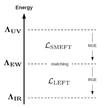
Figure 1: DsixTools 2.0 allows for a complete EFT computation between the high-energy scale $\Lambda_{\rm UV}$ and the low-energy scale $\Lambda_{\rm IR}$.

• User-friendly input handling

Even after fixing the operator basis for each EFT (Warsaw & San Diego), the user must choose a set of operators and make sure that the input values lead to a consistent Lagrangian. There are two types of inconsistencies:

1. Hermiticity: The Hermiticity of the Lagrangian imposes certain conditions on some WCs, and these must be respected by the input provided by the user. For instance, an input with $\left(C_{\ell q}^{(1)}\right)_{2223}\neq\left(C_{\ell q}^{(1)}\right)_{2232}^{\ast}$ would be inconsistent.

2. Antisimmetry: Some LEFT operators are antisymmetric under the exchange of two flavor indices and this implies that some WCs must be vanish. For instance, an input with $\left(L_{\nu\gamma}\right)_{11}\neq 0$ would be inconsistent.

In order to avoid potential issues associated to inconsistent inputs, DsixTools 2.0 includes user-friendly input routines that simplify the user’s task. The new version of DsixTools accepts input values for the WCs of any set of operators (belonging to the Warsaw or San Diego bases) and then checks for possible consistency problems. In the event of an inconsistency, DsixTools applies a change in the input to fix it and displays a warning message to inform the user. Furthermore, DsixTools transforms all Wilson coefficients to the symmetric basis, defined as the basis in which the WCs follow the same symmetry conditions as the associated operators. For instance, in this basis $\left(C_{\ell\ell}\right)_{1122}=\left(C_{\ell\ell}\right)_{2211}$ since $\left(Q_{\ell\ell}\right)_{1122}=\left(Q_{\ell\ell}\right)_{2211}$. This is the basis used internally by DsixTools. Nevertheless, the user needs not to worry about this, since the input/output is always unambiguous.

• More visual and easy to use

DsixTools 2.0 aims at a simpler and more visual experience. Many changes and simplifications of the package have been applied in order to guarantee this. In this new version, the user will be able to obtain the same results with much shorter programs than before. For instance, a complete program with a full EFT computation between the high-energy scale $\Lambda_{\rm UV}$ and the low-energy scale $\Lambda_{\rm IR}$ can now be written with only 6 lines of code. This is possible thanks to new routines that include automatic multi-step calculations. Moreover, a new Dictionary routine is available. This routine displays a large amount of useful information on any WC or operator of the SMEFT or the LEFT specified by the user. Along the same lines, a more intuitive naming for the SMEFT WCs is used in DsixTools 2.0 and more informative error messages are displayed. Finally, DsixTools 2.0 also contains an improved documentation. In addition to a printable manual, a comprehensive documentation system, fully integrated in Mathematica, is also available for the user right after installing the package.

• Evolution matrix formalism

Last but not least, DsixTools 2.0 implements a new and much faster method to solve the SMEFT and LEFT RGEs. This new approach is based on an evolution matrix formalism.

In order to understand the new method one can consider the case of the SMEFT, the application to the LEFT being analogous. The SMEFT RGEs can be generically written as (with $t\equiv\ln\mu$)

$$\frac{d\hat{C}_{i}(t)}{dt} =\frac{1}{16\pi^{2}}\,\hat{\gamma}_{ij}(\hat{C}_{k},C_{k})\,\hat{C}_{j}(t)\,,$$ (47)

$$\frac{dC_{i}(t)}{dt} =\frac{1}{16\pi^{2}}\,\gamma_{ij}(\hat{C}_{k})\,C_{j}(t)\,,$$ (48)

where $\gamma$ is the anomalous dimensions matrix (ADM). Quantities associated to dimension-four ($d=4$) objects are denoted with a hat, while the non-hatted quantities correspond to the dimension-five and -six ($d>4$) ones. These form a system of coupled differential equations. However, one must note that, at first order in the EFT expansion, the ADM for the $d>4$ operators only depend on $\hat{C}_{k}$. Therefore, since $C_{k}\sim 1/\Lambda_{\rm UV}^{2}$, the first equation above can be written as

$$\frac{d\hat{C}_{i}(t)}{dt}=\frac{1}{16\pi^{2}}\,\hat{\gamma}_{ij}(\hat{C}_{k})\,\hat{C}_{j}(t)+\mathcal{O}(1/\Lambda_{\rm UV}^{2})\,,$$ (49)

which corresponds to the Standard Model RGE evolution. These equations are known up to 3-loops and can be solved numerically relatively fast, since they only involve the $d=4$ sub-block, leading to

$$\hat{C}_{k}(t)=C_{k}^{\rm SM}(t)+\mathcal{O}(1/\Lambda_{\rm UV}^{2})\,,$$ (50)

where $C_{k}^{\rm SM}(t)$ are interpolating functions obtained by the numerical RGE solution. One can now plug this into Eq. (48) to write

$$\frac{dC_{i}(t)}{dt}=\frac{1}{16\pi^{2}}\,\gamma_{ij}(C_{k}^{\rm SM})\,C_{j}(t)+\mathcal{O}(1/\Lambda_{\rm UV}^{2})\equiv\bar{\gamma}_{ij}(t)\,C_{j}(t)+\mathcal{O}(1/\Lambda_{\rm UV}^{2})\,,$$ (51)

so that the ADM is now a function of $t$ only. Therefore, the resulting equation can be solved in terms of an evolution matrix $U\sim\exp\left(\bar{\gamma}\right)$, such that

$$C_{i}(t)=U_{ij}(t,t_{0})\,C_{j}(t_{0})\,.$$ (52)

Finally, once the $C_{i}(t)$ solutions have been found, they can be plugged into the equations for the $d=4$ parameters. Given the small number of $d=4$ operators, these can be solved numerically quite fast, obtaining in this way a full $\mathcal{O}(1/\Lambda_{\rm UV}^{2})$ solution of the system.

9 Wilson/WCxf

Speaker: Speaker Jacky Kumar
University of Montreal

To study the low energy phenomenology in a model using SMEFT, the first step is to match the model at the high scale $\Lambda$ to the effective operators $\mathcal{O}_{i}$ of SMEFT, then to run down the SMEFT operators to the electroweak scale, match them onto the WET operators $O_{i}$ and then further run them down to the mass of the bottom quark or some other low scale depending on the process that we are interested in. Once we have the Wilson coefficients at a given scale the next step is to calculate the observables of interest in terms of these Wilson coefficients. These steps are visualized in Fig.2.

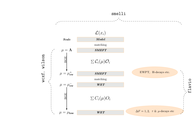
Figure 2: The standard steps involved in a phenomenological analysis using SMEFT and packages to perform these steps.

The aim of the python program wilson[14] is to automate the running, matching and translating the bases of Wilson coefficients in SMEFT and WET. The wilson package is built upon the Wilson coefficient exchange format(wcxf)[36]. It can be used together with packages like flavio[18] for predictions of observables, smelli[16] for global fits to carryout a complete phenomenological analysis using SMEFT, or for clustering analyses using the Python package ClusterKinG [62].

wcxf is a data exchange format for the numerical values of Wilson coefficients which helps interfacing different packages used in particle physics. For example model-specific Wilson coefficient calculators, renormalization group (RG) runners, and observable calculators etc.

The important features of wcxf are:

• Unambiguous: it uses a non-redundant set of operators and a fixed normalization for each basis.

• Extensible: it allows the addition of new EFTs and bases by the user.

• Robust: it is based on yaml and JSON files.

The format is defined in terms of three kinds of files:

• The EFT file, which is immutable, fixing the theory such as SMEFT or WET.

• The basis file, which is also immutable, defining the basis by listing all non-vanishing operators. Examples include the Warsaw or flavio basis.

• The Wilson coefficient file, which contains the actual data i.e the numerical values of Wilson coefficients at a given scale for an EFT in some basis.

In the current version of the program, the SMEFT and WET, WET-4, WET-3, WET-2 are implemented. Here the various WETs differ in the number of quark and lepton flavours. Furthermore, for the SMEFT the Warsaw [2], Warsaw up and Warsaw mass[50] bases and for WET the JMS, Bern, flavio, formflavor, FlavorKit and EOS bases are predefined.

The wilson package uses the Wilson coefficient exchange format. Given the numerical values of the Wilson coefficients at a given scale it can perform:

• Running of the complete set of dimension six SMEFT operators
  (based on DsixTools [13]).

• Matching (tree level) of SMEFT onto WET for all operators.

• Running of the complete set of dimension six WET operators.

• Translation of bases in SMEFT and WET.

The implementation of wilson based on the following work:

• The 1-loop SMEFT RGEs are based on anomalous dimension calculations of Refs[46, 44, 45].

• The tree level SMEFT onto WET matching is based on the calculations performed in Refs[50, 5].

• The 1-loop (QCD, QED) WET running is based on Refs[4, 43].

To install wilson and wcxf, one has to execute the following commands in the terminal:

python3 -m pip install wilson --user

python3 -m pip install wcxf --user

For further information and updates about wilson and wcxf we refer to the project websites https://wilson-eft.github.io/ and https://wcxf.github.io/ respectively.

10 The SMEFTsim package

Speaker: Ilaria Brivio
Institut für Theoretische Physik, Universität Heidelberg

10.1 Motivation and scope

The SMEFTsim package [19] is mainly designed for enabling global SMEFT analyses at the LHC. It is available at feynrules.irmp.ucl.ac.be/wiki/SMEFT. The users are encouraged to check periodically this repository for updates.

SMEFTsim is a FeynRules and UFO implementation of the full set of dimension-6, baryon number conserving operators of the Warsaw basis [2]. It allows the parton-level Monte Carlo simulation of arbitrary processes in the presence of SMEFT operators.

Its main scope is the estimation of leading SMEFT corrections to SM observables: it is not equipped for NLO evaluations and the effective Lagrangian is truncated at order $\Lambda^{-2}$, corresponding to a numerical accuracy of a few % for $C_{i}\sim 1$ and $\Lambda\gtrsim 1$ TeV. Note that, for this reason, complete and fully consistent results are only ensured for $\mathcal{O}(\Lambda^{-2})$ contributions.

10.2 Implementation

The SMEFTsim package contains the FeynRules input files and a set of pre-exported UFO models. The latter have been optimized for MadGraph5_aMC@NLO but are compatible with most Monte Carlo generators.

The SMEFT Lagrangian is implemented in the fermion basis where the $d$ quark masses are diagonal. The gauge fields are rescaled to bring their kinetic terms to canonical form and the SM parameters are automatically redefined to account for SMEFT corrections to the input measurements.The Lagrangian and analytic Feynman rules can be accessed with the Mathematica notebook supplied. The model is not equipped for NLO simulations and gauge choices other than the unitary gauge are not fully supported.

In order to reproduce all the main Higgs production and decay channels in the SM, the loop-induced Higgs couplings ($hGG,\,h\gamma\gamma,\,hZ\gamma$) are implemented as effective vertices with couplings given by the SM $t$- and $W$-loops evaluated for on-shell external bosons.

Interaction orders are defined in order to control the interactions to be included in the Monte Carlo generation. In addition to the customary QCD and QED orders, all SMEFT vertices have an interaction order NP=1, and the SM loop-induced Higgs couplings have order SMHLOOP=1. In MadGraph5_aMC@NLO one can evaluate e.g. the pure SM-SMEFT interference terms with the syntax NP^2 == 1.

SMEFTsim supports the WCxf exchange format [36] via a python script that converts a WCxf input file into a param_card for the UFO models.

Implemented frameworks

SMEFTsim comes in 6 different implementations, that differ in flavor assumptions (3 options) and input parameter scheme (2 options).

The flavor assumptions currently available are the following:

• the most general structure, where all flavor indices are free. This setup contains 2499 SMEFT parameters.

• a $U(3)$ symmetry is assumed for each of the 5 fermion fields of the SM ($q,l,u,d,e$), resulting in a $U(3)^{5}$-symmetric Lagrangian. Yukawa couplings are taken to be spurions of this symmetry, and only terms with up to 1 Yukawa insertion are retained. This scenario is the most restrictive and contains 81 SMEFT parameters.

• a linear Minimal Flavor Violation ansatz: the CP and $U(3)^{5}$ symmetries of the Lagrangian are assumed to be violated only due the breaking sources of the SM, i.e. the CKM complex phase and the Yukawa couplings. CP violation in purely bosonic operators are suppressed proportional to the Jarlskog invariant $J\sim 3\cdot 10^{-5}$ and are therefore neglected. Flavor symmetric spurion insertions up to $\mathcal{O}(y_{b}^{2},y_{t}^{2})$ are retained, in contrast with the U35 setup where only the leading, Yukawa-indepedent terms are included. This models contains 129 independent parameters.

The input parameters sets implemented are $\{\alpha_{em},m_{Z},G_{F}\}$ (which is labeled alphaScheme) and $\{m_{W},m_{Z},G_{F}\}$ (labeled MwScheme), where $m_{W,Z}$ are the masses of the electroweak bosons, $G_{F}$ is the Fermi constant and $\alpha_{em}$ the fine structure constant. These two sets provide alternative choices for fixing the numerical values of the 3 free parameters of the electroweak gauge sector of the SM (that can be chosen to be e.g. $\{g,g^{\prime},v\}$). In addition to these, the Higgs mass is used to fix the remaining free parameter in the scalar potential and the fermions’ masses to fix the Yukawa couplings (an input scheme for the CKM matrix can also be defined [63], although this is not currently implemented in SMEFTsim). As the input measurements are generically affected by dimension 6 operators, the SM parameters inferred from them are correspondingly shifted, so that a net discrepancy between an input and a predicted measurement is formally moved to the latter (see e.g. Refs. [64, 19] for further details). Such parameter shifts are automatically included in the SMEFTsim Lagrangian.

Restriction cards are provided within each UFO model, that can be used e.g. to set to zero light fermion masses or to recover the SM limit. Further ad hoc restrictions can be easily added by the user.

10.3 Validation

SMEFTsim has been validated in several ways. Most notably:

• with an internal validation. Two independent complete versions (set A and set B) were created, whose output was compared for a large number of processes. Both sets are available online for cross-checks.

• against dim6top for the subset of operators containing a top quark. All the tables in Ref. [65] were derived independently with the two UFO models.

• against both dim6top and SMEFT@NLO  using the validation tools and procedure recommended by the LHC Top and Electroweak Working Groups and by the LHC Higgs Cross Section Working Group [66].

• against a number of expressions derived with independent analytic calculations, in particular for EW and Higgs observables at LEP and at the LHC (e.g. those in [67, 68]).

11 The SMEFiT fitting code

Speaker: Emma Slade
Rudolf Peierls Centre for Theoretical Physics, University of Oxford

The effects of dimension-6 operators in the SMEFT can be written as:

$$\sigma=\sigma_{\rm SM}+\sum_{i}^{N_{d6}}\kappa_{i}\frac{c_{i}}{\Lambda^{2}}+\sum_{i,j}^{N_{d6}}\widetilde{\kappa}_{ij}\frac{c_{i}c_{j}}{\Lambda^{4}}\,,$$ (53)

where $\sigma_{\rm SM}$ indicates the SM prediction and $c_{i}$ are the Wilson coefficients we wish to constrain. In this work we develop a novel strategy for global SMEFT analyses [15], which we denote by SMEFiT. As a proof of concept of the SMEFiT methodology, we apply it here to the study of top quark production at the LHC in the SMEFT framework at dimension-6. We adopt the Minimal Flavour Violation (MFV) hypothesis [69] in the quark sector as the baseline scenario, impose a $U(2)_{q}\times U(2)_{u}\times U(2)_{d}$ flavour symmetry in the first two generations and consider CP-even operators, ending up with 34 degrees of freedom.

We adopt the Monte Carlo (MC) replica method as it does not make any assumption about the probability distribution of the coefficients, and is not limited to Gaussian distributions. Given an experimental measurement of a cross-section, denoted by $\mathcal{O}_{i}^{\rm(exp)}$, with total uncorrelated uncertainty $\sigma_{i}^{\rm(stat)}$, $N_{\rm sys}$ correlated systematic uncertainties $\sigma^{\rm(sys)}_{i,\alpha}$, and $N_{\rm norm}$ normalisation uncertainties $\sigma^{\rm(norm)}_{i,n}$, the artificial replicas are generated as

$$\mathcal{O}_{i}^{(\mathrm{art})(k)}=S_{i,N}^{(k)}\mathcal{O}_{i}^{\mathrm{(}\mathrm{exp})}\bigg{(}1+r_{i}^{(k)}\sigma_{i}^{\rm(stat)}+\sum_{\alpha=1}^{N_{\rm sys}}r_{i,\alpha}^{(k)}\sigma^{\rm(sys)}_{i,\alpha}\bigg{)}\ ,\quad k=1,\ldots,N_{\mathrm{rep}}\ ,$$ (54)

where the index $i$ runs from 1 to $N_{\rm dat}$ and where $S_{i,N}^{(k)}$ is a normalisation term. In order to ensure that no residual MC fluctuations remain, we will use $N_{\rm rep}=1000$ as our baseline. For each MC replica, the corresponding best-fit values are determined from the minimisation of a figure of merit

$$E(\{c_{l}^{(k)}\})\equiv\frac{1}{N_{\rm dat}}\sum_{i,j=1}^{N_{\rm dat}}\left(\mathcal{O}^{(\rm th)}_{i}\left(\{c_{l}^{(k)}\}\right)-\mathcal{O}^{{(\rm art)}(k)}_{i}\right)({\rm cov}^{-1})_{ij}\left(\mathcal{O}^{(\rm th)}_{j}\left(\{c_{l}^{(k)}\}\right)-\mathcal{O}^{{(\rm art)}(k)}_{j}\right)\;,$$ (55)

where $\mathcal{O}^{(\rm th)}_{i}$ is the theoretical prediction for the $i-$th cross-section evaluated using the $\{c_{l}^{(k)}\}$ values for the Wilson coefficients. The final fit quality can be quantified with the $\chi^{2}$

$$\chi^{2}\equiv\frac{1}{N_{\rm dat}}\sum_{i,j=1}^{N_{\rm dat}}\left(\mathcal{O}^{(\rm th)}_{i}\left(\{\langle c_{l}\rangle\}\right)-\mathcal{O}^{(\rm exp)}_{i}\right)({\rm cov}^{-1})_{ij}\left(\mathcal{O}^{(\rm th)}_{j}\left(\{\langle c_{l}\rangle\}\right)-\mathcal{O}^{(\rm exp)}_{j}\right)\;,$$ (56)

where now the theoretical predictions, computed using the expectation value for the degree of freedom $c_{l}$, are compared to the central experimental data. This is evaluated as the average over the resulting MC best-fit sample $\{c_{l}^{(k)}\}$.

We use as input to all our theory calculations the NNPDF3.1 NNLO no-top PDF set [70], to prevent us double-counting the data both in the PDFs and the SMEFT fits. To account for the removal of the data in the PDF fit, we include PDF uncertainties in the covariance matrix. We use NNLO QCD predictions for all available SM processes, and NLO otherwise. We also use MC cross-validation to prevent over-fitting the coefficients, and implement closure tests to ensure a rigourous test of the SMEFiT methodology.

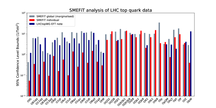
Figure 3: The 95% CL bounds on the 34 degrees of freedom included in SMEFiT, both in the marginalised and in the individual fit cases, with the bounds reported in the LHC Top WG EFT note [65]. The definitions of the degrees of freedom is given in Ref. [15].

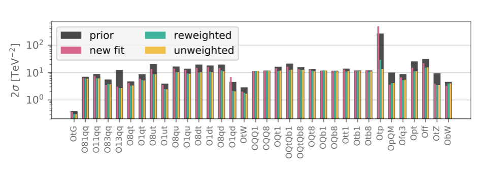
Figure 4: The 95% CL bounds for the $N_{\rm op}=34$ Wilson coefficients considered in the SMEFiT reweighting analysis of the top quark sector.

In Fig. 3 we show the 95% CL bounds on the 34 degrees of freedom considered in [15] both at the marginalised and individual-fit level. Within finite-size uncertainties, we find, as expected, the individual bounds to be tighter than the global bounds, as correlations between degrees of freedom are ignored in the former. Some of us have reported [71] on the applicability of the Bayesian reweighting technique developed for fitting Parton Distribution Functions [72, 73]. This method has two advantages in comparison to a fit to new data: it is essentially instantaneous, and it can be carried out without access to the SMEFT fitting code. We show in Fig. 4 the prior results without any single-top data included with those after $t$-channel measurements have been added either by reweighting or by performing a new fit. We find that, under well-defined conditions, the results obtained with reweighting all the single-top $t$-channel data are equivalent to those obtained with a new fit to the extended set of data.

12 Flavour Physics with EOS

Speaker: Danny van Dyk
Technische Universität München

Within the Standard Model (SM) of particle physics, changes of flavour quantum numbers follow stringent rules. Tree-level processes can change flavour only in charged-current processes, while neutral-current processes emerge first at the one-loop level and are thus suppressed. The coupling strengths of both types of processes are governed exclusively by the Yukawa couplings. Measurements of flavour-changing processes therefore provide means to determine most of the Standard Model (SM) parameters, but also place stringent constraints on possible effects beyond the Standard Model (SM) of particle physics [74]. While commonly used to bound the model parameters of UV-complete theories that could replace the SM, constraints from flavour observables can also be used to distinguish between different models for the origin of flavour, and between different dynamics behind electroweak symmetry breaking [75]. With the absence of any direct hints of effects Beyond the SM (BSM), indirect flavour constraints have stirred increasing interest amongst model builders. It is therefore important to the flavour physics community to provide convenient and easy bridges toward using our results to the any and all interested parties. EOS is meant to be such a bridge.

The EOS software has been authored with three use cases in mind:

1. To produce accurate and precise theory predictions and uncertainty estimates of flavour observables and related theoretical quantities. EOS aspires to facilitate the production of these predictions and estimates with publication quality.

2. To infer a variety of parameters from experimental measurements and from theoretical constraints. For this task, EOS defaults to using a Bayesian statistical framework. For the convenience of the user, EOS ships with a database of measurements and further constraints that can be used immediately.

3. To produce pseudo events that are useful to carry out sensitivity studies for phenomenological and experimental analyses. EOS aspired to produce such pseudo events for direct use in experimental analyses.

To achieve the outcomes of these use cases as effectively as possible, EOS has been written as a C++14 software with Python3 bindings. It includes sophisticated Monte Carlo tools based on Markov chains and importance sampling [76] to tackle statistical analyses with $\mathcal{O}(100)$ parameters. Binary packages of EOS are available for a variety of Linux distributions, and EOS can be quickly installed on MacOS via the Homebrew package manager [77].

The Python3 interface is recommended to all novice users, and example notebooks using the Jupyter software [78] are available [79]. These examples showcase how to use EOS to carry out typical tasks to work on any of the use cases listed above. The examples use semileptonic decays of the type $\bar{B}\to D\ell\bar{\nu}$ to illustrate how to predict integrated and differential kinematical distributions, infer the SM parameter $|V_{cb}|$ and hadronic parameters, and generate pseudo events within the SM and for BSM benchmark points. A detailed write-up with additional explanations can be viewed on the EOS webpage page [80]. In figure 5, two example plots are presented that illustrate the capabilities of EOS with the Python3 interface.

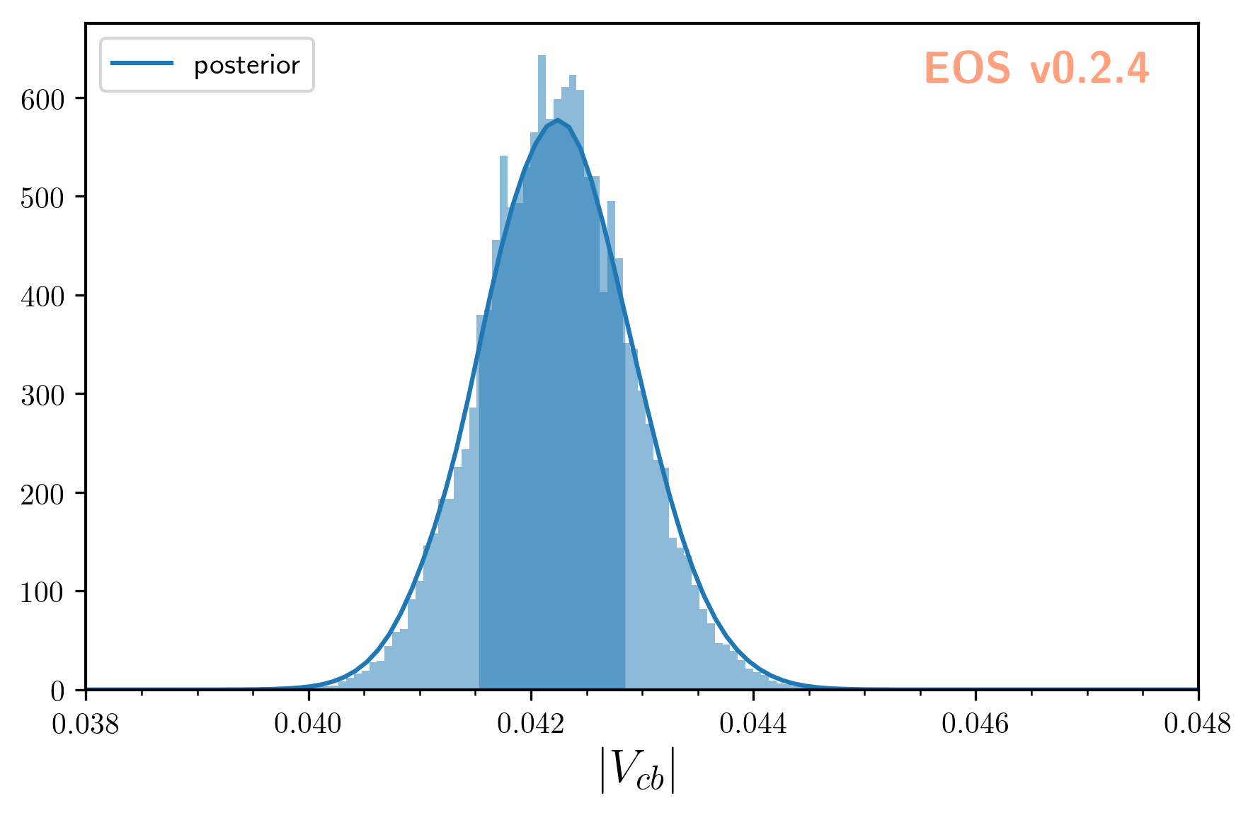
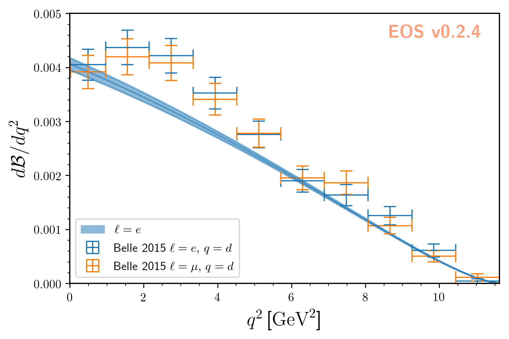
Figure 5: Two of the plots created by the example notebooks. Left: Histogram of random variates for $|V_{cb}|$ obtained and plotted with the EOS Python interface, overlaid with a kernel density estimate of the posterior probability density. Right: Uncertainty envelope at $68\%$ credibility of the posterior-prediction for the $\bar{B}\to De^{-}\bar{\nu}$ differential branching fraction as a function of $q^{2}$, the $e^{-}\bar{\nu}$ mass squared. The curves and bands are overlaid with data points by the Belle collaboration from measurements of the $\bar{B}\to De^{-}\bar{\nu}$ and $\bar{B}\to D\mu^{-}\bar{\nu}$ branching fraction in $q^{2}$ bins.

The EOS developers invest effort on providing precise and accurate predictions of flavour observables in and beyond the SM. Flavour observables are implemented independent of any concrete BSM model by using process-specific Weak Effective Theories (WETs). In this approach, a variety of hadronic matrix of local WET operator elements are needed. EOS allows to switch between different approaches for the evaluation of these hadronic matrix elements at run time. To connect low-energy flavour observables within their various WETs to one common high-energy BSM scenario within the Standard Model Effective Field Theory (SMEFT), matching and running between both theories is needed. To this end, EOS interfaces with the Wilson Python package [14] via the Wilson Coefficients exchange format [36].

13 flavio and smelli

Speaker: David M. Straub
Excellence Cluster Universe/TUM

flavio [18, 81] and smelli [16, 82] are two closely related open source Python packages.

flavio has the following main features:

• It is a general observable calculator (with uncertainties) in terms of WET or SMEFT Wilson coefficients,

• it contains a database of experimental meausurements,

• it allows the automated construction of likelihoods.

In addition, it contains convenient plotting routines, interfaces to fitters (MCMC), and a frequentist likelihood profiler.

smelli, the SMEFT Likelihood package, is built on top of flavio and provides a global likelihood in the space of SMEFT Wilson coefficients. The main motivation for smelli is:

• providing a consistent set of observables included in the likelihood,

• correct treatment of SM parameters in the presence of $D=6$ effects,

• construction of a nuisance-free likelihood,

• more informative presentation of results (table of observables with pulls etc.).

While flavio aims to be easy to modify and very flexible, the focus in smelli is on the ease of use and consistency rather than generality.

Thanks to the wilson package (Section 9), flavio, which originally started as a pure flavour physics package, now also supports electroweak precision tests and will soon add Higgs physics. In principle, every observable where new physics enters via Wilson coefficients of local operators can be added. The long term goal is to include all processes sensitive to dimension-6 SMEFT operators. Correspondingly, the long-term goal for smelli is to become truly global in constraining as many directions in SMEFT Wilson coefficient space as at all possible.

As of version 1.5, flavio includes the following classes of observables:

• $B$ physics: $B\to(V,P,X)\ell\ell$, $B\to\ell\ell$, $B\to(V,X)\gamma$, $\Lambda_{b}\to\Lambda\ell\ell$, $B\to(V,P,X)\ell\nu$, $B\to\ell\nu$, mixing

• $K$ physics: $K\to\pi\nu\nu$, $K\to\ell\ell$, $K\to\ell\nu$, $K\to\pi\ell\nu$, $\epsilon_{K}$, $\epsilon^{\prime}/\epsilon$

• $D$ physics: $D\to\ell\nu$, CPV in mixing

• $\mu$ physics: $\mu\to e\gamma$, $\mu\to 3e$, $\mu$-$e$ conversion, $\nu$ trident

• $\tau$ physics: $\tau\to 3\ell$, $\tau\to\ell\gamma$, $\tau\to(P,V)\ell$, $\tau\to V\nu$, $\tau\to\ell\nu\nu$

• EWPT: All LEP-1 $Z$ and $W$ pole observables

• Dipole moments: $(g-2)_{e,\mu,\tau}$, $d_{n}$

Near-future versions will add nuclear and neutron $\beta$ decays as well as Higgs production and decay.

Figure 6: Sketch of observables currently included in smelli’s global SMEFT likelihood.

smelli, as of version 1.3, includes every observable in flavio that fulfills two criteria: it has been measured and it is relevant for constraining SMEFT Wilson coefficients. The classes of observables are visualized in the sketch in figure 6. There are only two limitations at present. One is that semi-leptonic charged-current meson decays are not included yet, as the effect of new physics on CKM element extractions is not treated consistently yet. However, a solution similar to [63] has been implement in smelli and will be public soon. The second limitation is that the statistical approach used to be able to provide a nuisance-free likelihood (for details see [16]) does not allow to include observables where theory uncertainties are strongly dependent on new physics, as is the case e.g. for the neutron EDM or CP violation in $B\to DK$ decays. Ideas to solve this second limitation are being explored.

A brief interactive tutorial demonstrating the usage and main features of flavio and smelli can be found at the following URL:

https://github.com/DavidMStraub/flavio-smelli-mini-tutorials

An example of a possible application of the two codes is given by the well-known plot in figure 7, showing the interplay of charged- and neutral-current $B$ decays on semi-leptonic SMEFT Wilson coefficients, very relevant for the present $B$ “anomalies” [83].

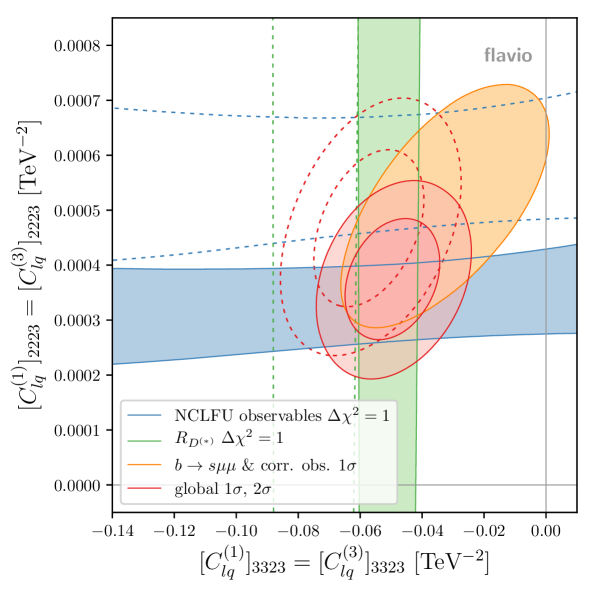
Figure 7: smelli global likelihood (and sub-likelihoods) in the plane of two SMEFT Wilson coefficients at the scale 2 TeV, plotted with flavio.plots. Taken from [83].

14 Matching the flavour symmetric SMEFT to flavour observables

Speaker: Sophie Renner
SISSA International School for Advanced Studies

This talk was based on Ref. [51].

14.1 Introduction

The success of the CKM picture of quark flavour mixing points towards there being no large sources of flavour breaking beyond the Standard Model (SM). If TeV-scale new physics exists, models with a flavour symmetry are therefore highly motivated. In the following I describe calculations of some of the most important flavour effects generated by flavour symmetric operators within the Standard Model Effective Field Theory (SMEFT).

14.2 Matching the $U(3)^{5}$ invariant SMEFT to WET coefficients up to one-loop

We select operators in the Warsaw Basis [2] of dimension 6 operators by starting from a $U(3)^{5}$ flavour symmetry defined as

$$U(3)_{q}\times U(3)_{u}\times U(3)_{d}\times U(3)_{l}\times U(3)_{e},$$ (57)

which is the largest global symmetry of the gauge sector of the SM Lagrangian, and under which the SM fermion fields transform in the fundamental of their corresponding $U(3)$, and as singlets under the others. We consider only the effects of operators which are overall singlets under this $U(3)^{5}$ symmetry, an assumption which essentially eliminates tree level flavour changing neutral currents (FCNCs). The motivations for this are as follows

• Will allow incorporation of flavour data into global SMEFT fits, which often use the same flavour assumption

• Approximates a “worst-case scenario” for the effects of TeV-scale new physics in flavour measurements, and thus represents an estimate of the irreducible flavour effects that might be expected

• Provides a starting point from which to explore other motivated flavour symmetries (e.g. less restrictive MFV scenarios, $U(2)^{5}$ in the first two generations, etc)

We match onto operators in the Weak Effective theory (WET) which generate some of the most sensitive flavour observables to new physics: semileptonic down-type FCNC decays (e.g. $B\to K^{(*)}l^{+}l^{-}$) and down-type meson mixing (e.g $B_{s}$-$\bar{B}_{s}$, $K^{0}$-$\bar{K}$). The flavour symmetry assumption ensures that there are no tree-level FCNCs induced by the SMEFT operators we consider, so matching at one-loop is necessary, with the flavour change arising from SM loops involving $W^{\pm}$ bosons. Examples of the diagrams involved are shown in Figure 8.

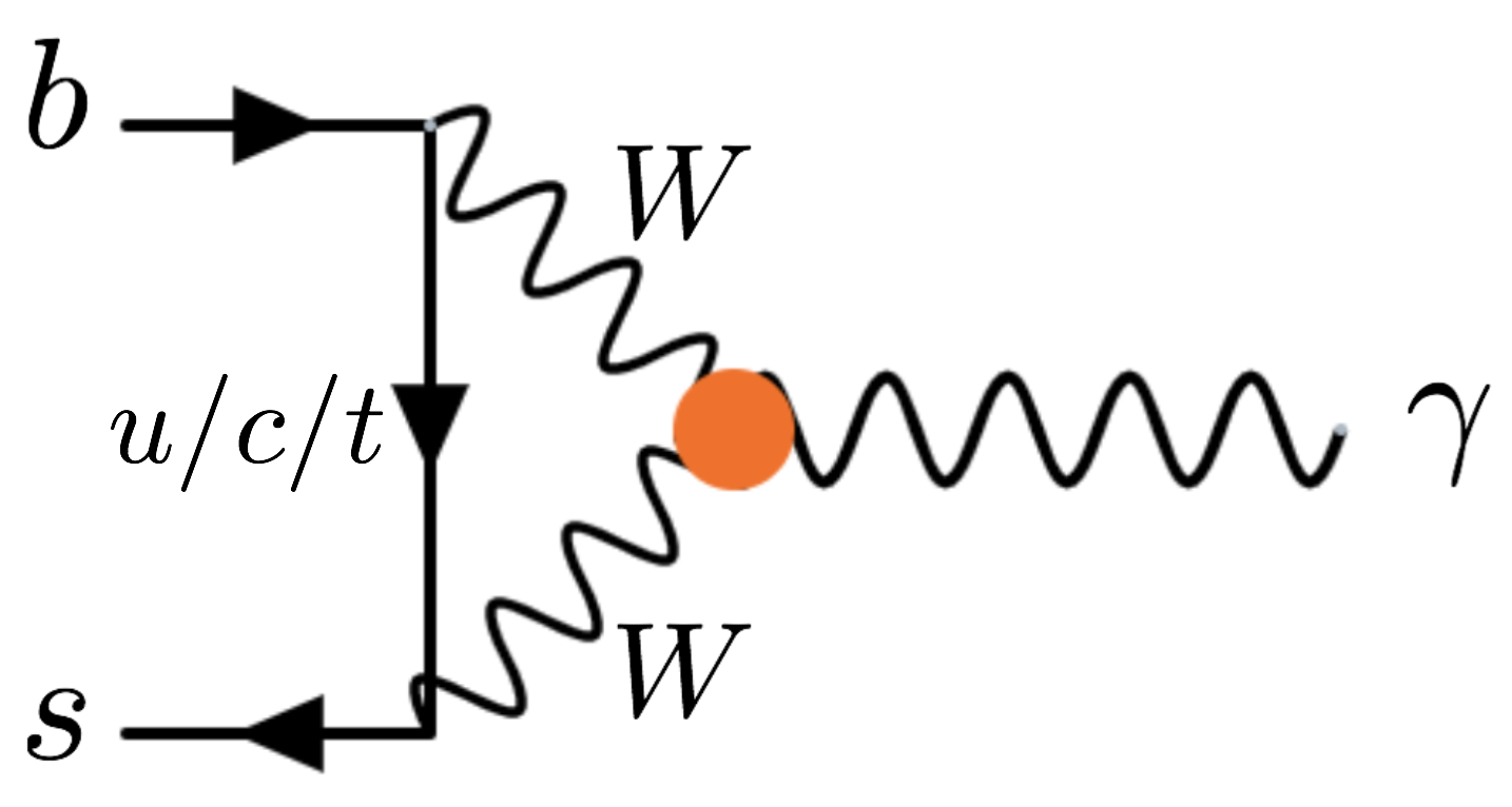
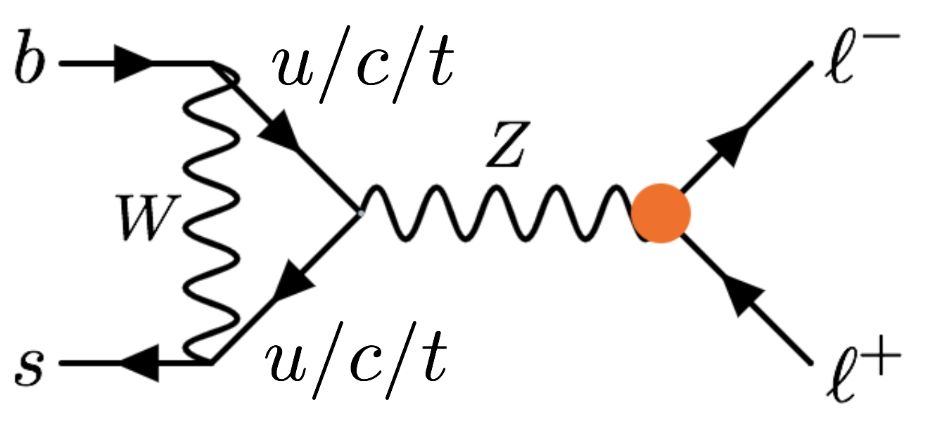
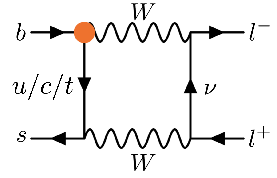
Figure 8: Examples of diagrams for one-loop matching, where the orange blobs represent insertions of SMEFT operators

14.3 Results and discussion

For results we refer to [51]. Here we point out a few general properties of the calculations. The $U(3)^{5}$ flavour symmetry we assume ensures that the results of the matching calculations share many properties with the SM, in particular:

• GIM mechanism: all results depend on $m_{t}$

• No right-handed currents: the matching only affects the coefficients of WET operators containing left-handed light quarks

• Same CKM factors: the matching produces effects with the same CKM suppressions as in the SM

Some of the operators we consider also enter into observables that are measured to fix the input parameters of the theory (see e.g. [84, 85, 67, 64]). We take these effects into account such that the results are written in terms of measured parameters, and present our results in two common schemes for the inputs fixing the electroweak sector of the theory: $\{m_{W},m_{Z},G_{F}\}$ and $\{\alpha,m_{Z},G_{F}\}$. Where possible, we compared results to those obtained previously in the literature [50, 86, 87, 88, 89, 90]. These calculations open up new possibilities for constraining the coefficients of SMEFT operators with flavour data.

15 MatchMaker

Speaker: José Santiago
CAFPE and University of Granada

15.1 Introduction

One of the (many) advantages of effective field theories (EFT) is that the comparison between experimental data and their implication in new physics models can be split in two independent steps. The bottom-up approach allows to parametrize in a maximally agnostic way the experimental data in terms of the Wilson coefficients of the corresponding EFT, without any relation to specific new physics models. The result is a global likelihood that can be computed thanks to the tools described elsewhere in this document. The top-down approach on the other hand introduces the necessary model discrimination by computing the Wilson coefficients in terms of the parameters of the new physics model.

The beauty of EFT is that it provides a power counting rationale to organize the model dependence inherent to the top-down approach, as the number of classes of models that contribute at a certain order in the perturbative expansion (loops and operator dimension) is finite. In this spirit, the complete classification of arbitrary extensions of the Standard Model (SM) that include new particles of spin smaller than 3/2 and contribute at tree level at the SM effective field theory (SMEFT) of dimension 6 has been recently achieved [31], building on previous partial efforts [91, 92, 93, 94]. Furthermore, technology allows us to automate this top-down approach , a necessary ingredient if we want to extend this complete classification beyond the tree-level approximation. This motivated us to develop MatchMaker, an automated tool to perform tree-level and one loop matching of arbitrary new physics models to the SMEFT.

15.2 MatchMaker: general philosophy

New physics models can be matched to an EFT either via functional methods, literally integrating out the heavy degrees of freedom directly in the path integral (see [95, 96, 97, 98, 99, 100, 101] for recent progress in this direction) or via a diagrammatic approach. This latter approach, in which off-shell 1-light-particle-irreducible (1lPI) Green functions are compared in the full model and the EFT, is the one used in MatchMaker.

MatchMaker relies on well established methods and tools for the process of tree-level and one-loop matching. It consists of a Python engine, which ensures that it is cross-platform, easy to install and flexible, and the following standard tools for the different steps of the calculation:

• FeynRules [102] is used to define the new physics model and to automatically compute the corresponding Feynman rules. Flavor indices are implicit dummy variables all through the calculation and therefore the number of generations is arbitrary with no computation penalty.

• QGRAF [103] is used to generate all the relevant amplitudes in the full and effective theories. These amplitudes are automatically dressed by MatchMaker with the Feynman rules computed in the previous step.

• The actual calculation of the corresponding amplitudes is performed with FORM [104]. This includes external momentum expansion, tensor reduction, partial fractioning, Dirac algebra and integration by part identities. All the calculations are done in dimensional regularization following the $\overline{\mbox{MS}}$ renormalization scheme.

• Finally, the comparison of the amplitudes in the full and effective theories is performed using Mathematica and the final form of the Wilson coefficients is stored in a file.

A few comments regarding the procedure described above are in order. As we have mentioned, we perform an off-shell matching in which the external particles are not required to be on-shell (only full momentum conservation is imposed). The rationale behind this choice is that we can restrict the calculation to 1lPI Green functions, as opposed to full S-matrix elements, and that the full off-shell kinematic structure provides a highly non-trivial kinematic redundancy that we use to cross-check the results obtained by MatchMaker. The down-side of this choice is that redundant operators, those that can be eliminated by field redefinitions and do not contribute to physical observables, have to be included in the process of matching. In order to keep the number of operators to consider under control we use the background field version of the ’t Hooft-Feynman gauge [105] so that only gauge invariant operators have to be considered. Following our philosophy of maximum flexibility we have not fixed a particular basis of evanescent operators, leaving the user to choose such a basis. The results of the matching are given first in the full off-shell Green basis, including all the relevant redundant and evanescent operators. This also includes the matching effects on the effective operators of dimension smaller than 6 (including the operators in the SM Lagrangian). On top of this completely general result for the tree-level and one-loop matching, MatchMaker also provides the result of the matching in the Warsaw basis [2], assuming 4-dimensional properties for the gamma matrices to reduce the evanescent operators. The elimination of the redundant operators to the Warsaw basis is performed by means of the equations of motion of the dimension-4 Lagrangian, after canonical normalization of the fields and the inclusion of the corrections to this Lagrangian from the matching process.

MatchMaker uses the following tests to check the correctness of the produced results:

• Full off-shell kinematic and gauge dependence. Off-shell kinematics provides a powerful and highly non-trivial test of the matching. Similarly, all components in gauge space are independently checked.

• Ward identities. We carefully compare amplitudes with different number of external legs, in which a momentum is replaced with the corresponding gauge bosons, to check all the relevant Ward identities.

• Symmetry and hermiticity properties of the Wilson coefficients. Some Wilson coefficients have symmetry properties under the exchange of flavor indices, including in cases complex conjugation. These properties are systematically checked in the result of the matching.

15.3 Status and future prospects

At the time of this writing MatchMaker is not yet publicly available. We are finalizing the last checks of the program and we expect to make it public in the near future. The current version produces in an automated way the tree-level and one-loop matching of an arbitrary new physics model (with the only restriction that it has to be implementable in FeynRules) into the SMEFT, provided no fermion-number violating couplings are introduced in the model. We expect the latter to be handled in future versions of the program. The grand goal is to extend this tool to arbitrary effective Lagrangians.

16 Lepton dipole moments at two loops in the SMEFT

Speaker: Giovanni Marco Pruna
INFN, Sezione di Roma Tre

In the last decade, the absence of signals for physics beyond the Standard Model (BSM) at collider experiments, together with the increasing precision of both high- and low-energy experiments, corroborated the idea that there can be a considerable scale separation between the SM and New Physics, thus creating strong grounds for deeper studies of the Standard Model Effective Field Theory (SMEFT).

In fact, even though the SMEFT was introduced several decades ago [1], a systematic treatment of such theory above and below the electroweak symmetry-breaking (EWSB) scale was completed only a few years ago [2, 106, 5].

A similar fate occurred to the study of quantum fluctuations in SMEFT. Although many partial results had been presented in literature, a methodical analysis of the one-loop anomalous dimensions was only recently performed [44, 45, 46, 107, 43, 108].

Beyond the one-loop level, there are not many results, and these are not organised in a structured catalogue [109, 110, 111, 112, 113, 114, 115, 116, 117, 118, 119, 120, 121, 122, 123, 124]. However, the precision level that will be reached by future experiment will require a consistent knowledge of the two-loop leading contributions in SMEFT. Therefore, a collaborative effort is required to reach this goal in a reasonable time. It is beyond the scope of this document to analyse the phenomenological implications of a thorough knowledge of the two-loop anomalous dimensions in SMEFT. The focus instead is on the characteristic case of lepton dipole moments.

In the near future, a worldwide experimental plan will test such observables with unprecedented sensitivity. In two-to-five years, lepton-flavour violation (LFV) will be investigated in the muon sector with an increase of three orders of magnitude in sensitivity at the MEG II (PSI) [125], Mu3e (PSI) [126], COMET (J-PARC) [127] and Mu2e (FNAL) [128, 129] experiments. ACME II at Harvard University delivered a new result [130] on the electric dipole moment (EDM) of electrons with a significantly improved sensitivity. This year, the Muon $g-2$ experiment (FNAL) [131, 132] will also deliver exciting results on the anomalous magnetic moment of the muon ($a_{\mu}$), possibly addressing the nature of the long-standing discrepancy between measured and predicted values.

In this context, it has already been shown that a proper evaluation of the quantum fluctuations in SMEFT gives a deeper understanding of the phenomenological implications in searches for new physics [133, 47, 134, 135, 136, 137, 48, 138, 139, 140, 141, 142, 56, 49].

However, apart from the fact that evaluations of further loop levels would guarantee more control over the phenomenological interpretation, there is a formal subtlety that calls for a systematic determination of the two-loop leading contribution to the evolution/mixing of SMEFT operators.

In fact, it is well-known that matching an ultraviolet (UV) complete theory with its low-energy effective representation can distribute the leading contributions in different perturbative orders: the pioneering work on $b\rightarrow s\gamma$ transitions performed in the $1990$s revealed that this is a standard feature of the fermion dipole operators when quantum fluctuations are evaluated in an effective field theory [143, 144].

This aspect implies that the matching procedure performed at the one-loop level does not provide meaningful phenomenological information unless accompanied by a consistent evaluation of the anomalous dimensions at the two-loop level. This issue is made more radical by the fact that both the matching coefficient and the anomalous dimensions can depend on the regularisation scheme used to perform the aforementioned computation.

Therefore, the only way to remove all the scheme ambiguities from the correct phenomenological interpretation is to compute the anomalous dimensions at the two-loop level and the matching coefficients at the one-loop level in SMEFT, potentially in different regularisation schemes to cross-check the final outcome.

Other ambiguities can arise with the treatment of the antisymmetric Levi-Civita tensor in dimensional regularisation, and a careful implementation of the evanescent operator technology [109, 110, 113] is required.

The current level of automation allows implementation of the SMEFT Lagrangian in tools that can generate the relevant set of Feynman rules (e.g. FeynRules v2.3 [102]) to be interpreted by packages for multi-loop computations (e.g. FeynArts v3.11 [145] and FormCalc v9.8 [146, 147]). However, a completely automated chain is not yet available. For example, following the package chain that was just presented, one should notice that FormCalc struggles to deal with four-fermion operators. Therefore an intermediate Form file should be retained to be further elaborated off line in Form v4.2 [104].

Although it is not perfect, this strategy allows the non-integrated amplitudes to be further related to any effective operator by a projection algorithm. Dipole operators can be extracted with an off-shell projection [148].

After this, extracting the UV poles will require a strategy to regularise potential infrared (IR) divergences. In recent years, many techniques have been developed to this. However, all of these techniques involve rearranging the propagators into a tadpole integral, followed by a truncation that takes into account the superficial degree of divergence of the loop integral. One convenient choice is to rearrange every propagator with an IR mass regulator exactly [114, 116, 149]. Even though this approach is very efficient, it has the disadvantage that to be consistent one must add the new regulator mass in the original Lagrangian (possibly interfering with pre-existing masses) and carry out the potential set of counterterms that arise because of this insertion. Another choice is to add an artificial mass term to the massless gauge bosons and then expand the integral in the external momenta [148] (which is equivalent to an IR rearrangement into a multi-massive tadpole). Since two-loop tadpoles are very well-known objects [150, 151], this second method will also give a linear outcome. Hence the two methods can be considered equivalent.

The approach described in this section successfully reproduces the two-loop anomalous dimensions in $b\to s\gamma$ transitions below the EWSB scale in conventional dimensional regularisation [152], and can be adapted to compute the two-loop anomalous dimensions of lepton dipole moments with the operator basis presented in [5]. The result will appear in [153].

At current the state of the art, the procedure described here is surely one of the most efficient. However, there is no guarantee that it cannot be surpassed by interesting alternatives [154].

17 NLO corrections to $h\rightarrow b\bar{b}$ in the SMEFT

Speaker: Darren Scott
University of Amsterdam/Nikhef

Performing higher order perturbative corrections within the SMEFT can be important for at least two reasons. Not only do such corrections reduce the residual scale dependence in the resulting predictions as in the SM, but new Wilson coefficients can appear at NLO which are not present in the tree level result. On occasion these Wilson coefficients can have large numerical prefactors making them an important contribution when incorporated in a global fit. Some of these large contributions would not necessarily be captured by a standard RGE analysis thus making it necessary to compute the NLO corrections directly in order to properly capture the impact of such coefficients. This talk introduces NLO corrections to the decay $h\rightarrow b\bar{b}$ in the dimension-6 SMEFT [155, 156, 157], with emphasis on a number of complications or subtleties in the calculation of the dimension-6 decay rate which are not seen in the SM. We focus in particular on the renormalization of the electric charge, large NLO corrections (and the choice of renormalization scheme), and the use of decoupling relations. Further details can be found in [157] as well as the complete answer for the decay rate in Mathematica notebooks available with the arXiv submission.

In the on-shell scheme the electric charge is defined to be exactly equal to the tree level coupling of the $\gamma ff$-vertex at zero momentum transfer to the photon. The electric charge is universal, so the choice of $f$ does not affect the result one gets for the form of the counterterm $\delta e$. It can be shown that $\delta e$, using electroweak SM Ward identities, can be written (see e.g. [158])

$$\frac{\delta e}{e}=\frac{1}{2}\frac{\partial\Sigma_{T}^{AA}(k^{2})}{\partial k^{2}}\bigg{|}_{k^{2}=0}-\frac{(v_{f}-a_{f})}{Q_{f}}\frac{\Sigma_{T}^{AZ}(0)}{M_{Z}^{2}}\,,$$ (58)

where $\Sigma_{T}^{AB}$ is the transverse component of the $A\rightarrow B$ 2-point function, $v_{f}$ and $a_{f}$ are the vector and axial couplings of fermion $f$ to the Z-boson, and $Q_{f}$ is the electric charge of the fermion in units of $e$. In the SM, $v_{f}-a_{f}=-2Q_{f}\hat{s}_{w}/\hat{c}_{w}$ (where $\hat{s}_{w}$ and $\hat{c}_{w}$ are the sine and cosine of the weak mixing angle) making it clear that eq. (58) becomes independent of the choice of fermion used to compute $\delta e$. The naïve extension of eq. (58) to dimension-6 (i.e. including dimension-6 effects in $\Sigma_{T}^{AB}$, $v_{f}$, and $a_{f}$) leads to seemingly contradictory results. Specifically, for operators of the form $C_{Hf}(H^{\dagger}i\overleftrightarrow{D}_{\mu}H)(\bar{f}\gamma^{\mu}P_{R}f)$ where $H$ is the Higgs doublet with vacuum expectation value $\hat{v}_{T}$, one finds $v_{f}^{(6)}=-a_{f}^{(6)}=C_{Hf}\hat{v}_{T}^{2}/4\hat{c}_{w}\hat{s}_{w}$. Thus, this naïve extension leads to the result that the electric charge renormalization depends on fermion charge $Q_{f}$. One can of course avoid this issue by renormalizing the $\gamma ff$-vertex directly, without using the SM Ward identities, but it would be interesting to derive an all-orders equation analogous to eq. (58) which correctly takes into account dimension-6 terms.

Another issue is related to the origin of large NLO corrections in the results and their relation to the choice of renormalization scheme. We identify two such contributions; firstly those from QCD/QED type diagrams (those containing at least one gluon/photon) and secondly those from tadpole graphs containing a top quark or, to a lesser extent, a heavy boson. The former are smaller if one uses the $\overline{\text{MS}}$ scheme for the $b$-quark mass, while on the other hand tadpole contributions can be made to vanish if one instead uses the on-shell scheme everywhere. A solution to this apparent dilemma is through the use of decoupling relations. That is, we work in a scheme where the $b$-quark mass (and electric charge $e$) are defined in a low energy QCD$\times$QED theory with the top quark and heavy bosons decoupled (see e.g. [159]). We write the relation between the full theory $b$-quark mass in the $\overline{\text{MS}}$ scheme $\overline{m}_{b}(\mu)$ and the mass as defined in the low energy QCD$\times$QED theory $\overline{m}^{(\ell)}_{b}(\mu)$ as

$$\overline{m}_{b}(\mu)=\zeta_{b}(\mu,m_{t},m_{H},M_{W},M_{Z})\overline{m}^{(\ell)}_{b}(\mu)\,,$$ (59)

where the decoupling constant $\zeta_{b}$ captures the contributions from the top quark and heavy bosons to the $b$-quark mass. The decoupling constants can be calculated perturbatively through one-loop matching. The net effect is that the contributions from top quarks and heavy bosons are calculated in the on-shell scheme where the tadpole graphs cancel, while the QCD/QED contributions are calculated in the $\overline{\text{MS}}$ scheme where their contributions are smaller.

In this short text we have covered some issues related to electric charge renormalization and the use of decoupling relations when using a mix of on-shell and $\overline{\text{MS}}$ renormalization schemes to avoid anomalously large NLO corrections. There are some other subtleties not touched on here, such as Higgs-Z mixing, scale uncertainties, the flavour structure (see also [19, 46]), and gauge fixing (see also [37, 38, 39]) but which can also be found in the full paper [157] along with additional details on the points raised here.

18 (SM)EFT, thoughts about what everybody has seen

Speaker: Giampiero Passarino
Dipartimento di Fisica Teorica, Università di Torino

INFN, Sezione di Torino

There is increasing need to assess the impact and the interpretation of $\mathrm{dim}=6$ and $\mathrm{dim}=8$ operators within the context of the Standard Model Effective Field Theory (SMEFT [32]). The observational and mathematical consistency of a construct based on $\mathrm{dim}=6$ and $\mathrm{dim}=8$ operators should be critically examined  in the light of known theoretical results [160], including: local, non-local, hard and soft terms or why we should not forget loops [161] and Landau singularities; mixing, or why SMEFT may not be as general as we think; linear vs. quadratic EFT representations.

Non-local and all that

Consider the following scenario: the Standard Model (SM), valid for ${\mathrm{E}}\ll\Lambda$, the corresponding EFT extension (say SMEFT) and $X$, an UV completion of the SM (or the next theory in a tower of effective theories); we are interested in matching the low ${\mathrm{E}}$ limit of $X$ to the (SM)EFT. Non-local effects correspond to long distance propagation and hence to reliable predictions at low energy, local terms by contrast summarize the unknown effects from high energy: having both local and non-local terms allows us to implement the full (one-loop) EFT program [162]. Heavy-light terms describe a multi scale scenario: the light masses ($m_{i}$), the Mandelstam invariants characterizing the process ($s_{ij\dots k}$) and the heavy scale ($\Lambda$),

$$\Lambda^{2} \gg s_{ij\dots k}=-(p_{i}+p_{j}+\dots+p_{k})^{2}>(m_{1}+m_{2}+\dots+m_{n})^{2}\;\hbox{or}$$

$$\Lambda^{2} \gg \mid t\mid\;\gg m^{2}\,.$$

EFT mimics the unknown UV by matching the hard-local part of the loops, i.e.  the terms having a bounded number of derivatives. Soft-non local components in loops cancel on both sides of the matching condition but they are not a throwaway. The key advantage of including the non-local behavior is the appearance of some important kinematic dependence [162]. Important predictions of the EFT are often related to non-analytic contributions which modify tails of distributions.

Proliferation of scalars and mixing

The lack of discovery of beyond-the-SM (BSM) physics suggests that the SM is “isolated”, including small mixing between light and heavy scalars [163]: if there are many scalars then we have to assume that there is at least the same small mixing for every one of them.

SMEFT assumes a Higgs doublet, so any mixing among scalars (in general among heavy and light degrees of freedom) in the high-energy theory brings us to the HEFT/SMEFT dichotomy [32]. Although there is a wide class of BSM models that support the (linear) SMEFT description, this realization does not always provide the appropriate framework.

Mixing and low-energy limits

The choice of the heavy scale $\Lambda$ is crucial; in any BSM model the scale $\Lambda$ should not be confused with the mass of some heavy degrees of freedom – it is generally a ratio of masses and powers of couplings. The low energy behavior of underlying theory should be computed in the mass eigenbasis, not in the weak eigenbasis; mixing angles are function of $\Lambda$ and a large number of $1/\Lambda^{2}$ terms are due to the expansion of mixing angles, not to the integration of heavy fields [164].

In case deviations are observed, one needs to compare at the observable level (${\mathrm{O}}$) when interpreting the parameters of the underlying theory ($X$) . Comparison at the ${\mathrm{O}}$ level implies: in $X$, with parameters $\vec{p}$, compute an observable ${\mathrm{O}}^{i}={\mathrm{O}}^{i}_{X}(\vec{p})$. Perform a fit of the SMEFT coefficients ($\vec{{\mathrm{a}}}$) to a set of observables ($\vec{{\mathrm{O}}}$), that may but does not need to include ${\mathrm{O}}^{i}$. Take the best-fit coefficients ($\hat{\vec{{\mathrm{a}}}}$) from the fit above and compute the SMEFT-predicted observable, $\hat{{\mathrm{O}}^{i}}_{\rm{\scriptscriptstyle{SMEFT}}}={\mathrm{O}}^{i}_{\rm{\scriptscriptstyle{SMEFT}}}(\hat{\vec{a}})$. Perform a fit for the $X$ parameters $\vec{p}$ from the comparison to the SMEFT-predicted observable: $\hat{{\mathrm{O}}^{i}}_{\rm{\scriptscriptstyle{SMEFT}}}\sim{\mathrm{O}}^{i}_{X}(\vec{p})$. Should no deviations appear to arise from the SMEFT fit to data, $X$ comes into play. The result of a global SMEFT fit may yield $\hat{\vec{a}}\sim 0$. This can only be interpreted as “no deviations from SM under the SMEFT assumptions”, viz. that of a one doublet scalar sector.

Linear vs. quadratic EFT representation

Given the EFT amplitude ${\mathrm{A}}={\mathrm{A}}^{(4)}+\frac{1}{\Lambda^{2}}\,{\mathrm{A}}^{(6)}+\frac{1}{\Lambda^{4}}\,{\mathrm{A}}^{(8)}$ “linear” means including the interference between ${\mathrm{A}}^{(4)}$ and ${\mathrm{A}}^{(6)}$, “quadratic” currently means including the square of ${\mathrm{A}}^{(6)}$ and Not the complete inclusion of all terms giving $1/\Lambda^{4}$ (even before considering ${\mathrm{A}}^{(8)}$). Without $\mathrm{dim}=8$ the $1/\Lambda^{4}$ terms are basis-dependent.

In developing the (SM)EFT there is a dual motivation for including $\mathrm{dim}=8$ operators: it may prove that an analysis purely at the $\mathrm{dim}=6$ level is inadequate, or that $\mathrm{dim}=8$ effects should be accounted for as a systematic uncertainty. Indeed, given the plethora of new physics scenarios that may show up in future precision Higgs measurements only at the percent level, it is an urgent issue to understand and reduce theory uncertainties so that they do not become a limiting factor in our searches for new physics.

A continuum EFT is not a model, but a sequence of low-energy effective actions ${\mathrm{S}}_{{\mbox{\scriptsize{eff}}}}(\Lambda)$, for all $\Lambda<\infty$. EFT theories  are being widely used in an effort to interpret experimental measurements of SM processes [165]. In this scenario, various consistency issues arise; one should critically examine the issues and we argue for the necessity to learn more general lessons about new physics within the EFT approach; inconsistent results usually attributed to the EFTs are in fact the consequence of unnecessary further approximations.

References

- [1] W. Buchmuller and D. Wyler, “Effective Lagrangian Analysis of New Interactions and Flavor Conservation,” Nucl. Phys. B 268, 621 (1986).
- [2] B. Grzadkowski, M. Iskrzynski, M. Misiak and J. Rosiek, “Dimension-Six Terms in the Standard Model Lagrangian,” JHEP 1010, 085 (2010) [arXiv:1008.4884 [hep-ph]].
- [3] G. Buchalla, A. J. Buras and M. E. Lautenbacher, “Weak decays beyond leading logarithms,” Rev. Mod. Phys. 68, 1125 (1996) [hep-ph/9512380].
- [4] J. Aebischer, M. Fael, C. Greub and J. Virto, “B physics Beyond the Standard Model at One Loop: Complete Renormalization Group Evolution below the Electroweak Scale,” JHEP 1709, 158 (2017) [arXiv:1704.06639 [hep-ph]].
- [5] E. E. Jenkins, A. V. Manohar and P. Stoffer, “Low-Energy Effective Field Theory below the Electroweak Scale: Operators and Matching,” JHEP 1803, 016 (2018) [arXiv:1709.04486 [hep-ph]].
- [6] B. Gripaios and D. Sutherland, “DEFT: A program for operators in EFT,” JHEP 1901, 128 (2019) [arXiv:1807.07546 [hep-ph]].
- [7] J. C. Criado, “BasisGen: automatic generation of operator bases,” Eur. Phys. J. C 79, no. 3, 256 (2019) [arXiv:1901.03501 [hep-ph]].
- [8] J. Aebischer and P. Stangl, to be released soon.
- [9] A. Dedes, M. Paraskevas, J. Rosiek, K. Suxho and L. Trifyllis, “SmeftFR - Feynman rules generator for the Standard Model Effective Field Theory,” arXiv:1904.03204 [hep-ph].
- [10] J. C. Criado, “MatchingTools: a Python library for symbolic effective field theory calculations,” Comput. Phys. Commun. 227, 42 (2018) [arXiv:1710.06445 [hep-ph]].
- [11] C. Anastasiou, A. Carmona, A. Lazopoulos and J. Santiago, to be released soon.
- [12] S. Das Bakshi, J. Chakrabortty and S. K. Patra, “CoDEx: Wilson coefficient calculator connecting SMEFT to UV theory,” Eur. Phys. J. C 79, no. 1, 21 (2019) [arXiv:1808.04403 [hep-ph]].
- [13] A. Celis, J. Fuentes-Martin, A. Vicente and J. Virto, “DsixTools: The Standard Model Effective Field Theory Toolkit,” Eur. Phys. J. C 77, no. 6, 405 (2017) [arXiv:1704.04504 [hep-ph]].
- [14] J. Aebischer, J. Kumar and D. M. Straub, “Wilson: a Python package for the running and matching of Wilson coefficients above and below the electroweak scale,” Eur. Phys. J. C 78, no. 12, 1026 (2018) [arXiv:1804.05033 [hep-ph]].
- [15] N. P. Hartland, F. Maltoni, E. R. Nocera, J. Rojo, E. Slade, E. Vryonidou and C. Zhang, JHEP 1904, 100 (2019) doi:10.1007/JHEP04(2019)100 [arXiv:1901.05965 [hep-ph]].
- [16] J. Aebischer, J. Kumar, P. Stangl and D. M. Straub, “A Global Likelihood for Precision Constraints and Flavour Anomalies,” Eur. Phys. J. C 79, no. 6, 509 (2019) [arXiv:1810.07698 [hep-ph]].
- [17] D. van Dyk and others, “EOS — A HEP program for Flavor Observables”, https://eos.github.io.
- [18] D. M. Straub, “flavio: a Python package for flavour and precision phenomenology in the Standard Model and beyond,” arXiv:1810.08132 [hep-ph].
- [19] I. Brivio, Y. Jiang and M. Trott, “The SMEFTsim package, theory and tools,” JHEP 1712, 070 (2017) [arXiv:1709.06492 [hep-ph]].
- [20] R. Slansky, “Group Theory for Unified Model Building,” Phys. Rept. 79, 1 (1981).
- [21] L. Lehman and A. Martin, “Hilbert Series for Constructing Lagrangians: expanding the phenomenologist’s toolbox,” Phys. Rev. D 91, 105014 (2015) [arXiv:1503.07537 [hep-ph]].
- [22] B. Henning, X. Lu, T. Melia and H. Murayama, “Hilbert series and operator bases with derivatives in effective field theories,” Commun. Math. Phys. 347, no. 2, 363 (2016) [arXiv:1507.07240 [hep-th]].
- [23] L. Lehman and A. Martin, “Low-derivative operators of the Standard Model effective field theory via Hilbert series methods,” JHEP 1602, 081 (2016) [arXiv:1510.00372 [hep-ph]].
- [24] B. Henning, X. Lu, T. Melia and H. Murayama, “2, 84, 30, 993, 560, 15456, 11962, 261485, …: Higher dimension operators in the SM EFT,” JHEP 1708, 016 (2017) Erratum: [JHEP 1909, 019 (2019)] [arXiv:1512.03433 [hep-ph]].
- [25] H. D. Politzer, “Power Corrections at Short Distances,” Nucl. Phys. B 172, 349 (1980).
- [26] C. Arzt, “Reduced effective Lagrangians,” Phys. Lett. B 342, 189 (1995) [hep-ph/9304230].
- [27] J. C. Criado and M. Pérez-Victoria, “Field redefinitions in effective theories at higher orders,” JHEP 1903, 038 (2019) [arXiv:1811.09413 [hep-ph]].
- [28] H. Georgi, “On-shell effective field theory,” Nucl. Phys. B 361, 339 (1991).
- [29] B. Grzadkowski, Z. Hioki, K. Ohkuma and J. Wudka, “Probing anomalous top quark couplings induced by dimension-six operators at photon colliders,” Nucl. Phys. B 689, 108 (2004) [hep-ph/0310159].
- [30] J. A. Aguilar-Saavedra, “A Minimal set of top-Higgs anomalous couplings,” Nucl. Phys. B 821, 215 (2009) [arXiv:0904.2387 [hep-ph]].
- [31] J. de Blas, J. C. Criado, M. Perez-Victoria and J. Santiago, “Effective description of general extensions of the Standard Model: the complete tree-level dictionary,” JHEP 1803, 109 (2018) [arXiv:1711.10391 [hep-ph]].
- [32] I. Brivio and M. Trott, “The Standard Model as an Effective Field Theory,” Phys. Rept. 793, 1 (2019) [arXiv:1706.08945 [hep-ph]].
- [33] A. Falkowski, B. Fuks, K. Mawatari, K. Mimasu, F. Riva and V. Sanz, “Rosetta: an operator basis translator for Standard Model effective field theory,” Eur. Phys. J. C 75, no. 12, 583 (2015) [arXiv:1508.05895 [hep-ph]].
- [34] E. Anderson, Z. Bai, C. Bischof, L. S. Blackford, J. Demmel, J. J. Dongarra et al., LAPACK Users’ Guide (Third Ed.). Society for Industrial and Applied Mathematics, Philadelphia, PA, USA, 1999, http://www.netlib.org/lapack/lug/.
- [35] F. Sannino, P. Stangl, D. M. Straub and A. E. Thomsen, “Flavor Physics and Flavor Anomalies in Minimal Fundamental Partial Compositeness,” Phys. Rev. D 97, no. 11, 115046 (2018) [arXiv:1712.07646 [hep-ph]].
- [36] J. Aebischer et al., “WCxf: an exchange format for Wilson coefficients beyond the Standard Model,” Comput. Phys. Commun. 232, 71 (2018) [arXiv:1712.05298 [hep-ph]].
- [37] A. Dedes, W. Materkowska, M. Paraskevas, J. Rosiek and K. Suxho, “Feynman rules for the Standard Model Effective Field Theory in Rξ -gauges,” JHEP 1706, 143 (2017) [arXiv:1704.03888 [hep-ph]].
- [38] A. Helset, M. Paraskevas and M. Trott, “Gauge fixing the Standard Model Effective Field Theory,” Phys. Rev. Lett. 120, no. 25, 251801 (2018) [arXiv:1803.08001 [hep-ph]].
- [39] M. Misiak, M. Paraskevas, J. Rosiek, K. Suxho and B. Zglinicki, “Effective Field Theories in Rξ gauges,” JHEP 1902, 051 (2019) [arXiv:1812.11513 [hep-ph]].
- [40] F. Feruglio, “The Chiral approach to the electroweak interactions,” Int. J. Mod. Phys. A 8, 4937 (1993) [hep-ph/9301281].
- [41] B. Grinstein and M. Trott, “A Higgs-Higgs bound state due to new physics at a TeV,” Phys. Rev. D 76, 073002 (2007) [arXiv:0704.1505 [hep-ph]].
- [42] E. Fermi, “Trends to a Theory of beta Radiation. (In Italian),” Nuovo Cim. 11, 1 (1934).
- [43] E. E. Jenkins, A. V. Manohar and P. Stoffer, “Low-Energy Effective Field Theory below the Electroweak Scale: Anomalous Dimensions,” JHEP 1801, 084 (2018) [arXiv:1711.05270 [hep-ph]].
- [44] E. E. Jenkins, A. V. Manohar and M. Trott, “Renormalization Group Evolution of the Standard Model Dimension Six Operators I: Formalism and lambda Dependence,” JHEP 1310, 087 (2013) [arXiv:1308.2627 [hep-ph]].
- [45] E. E. Jenkins, A. V. Manohar and M. Trott, “Renormalization Group Evolution of the Standard Model Dimension Six Operators II: Yukawa Dependence,” JHEP 1401, 035 (2014) [arXiv:1310.4838 [hep-ph]].
- [46] R. Alonso, E. E. Jenkins, A. V. Manohar and M. Trott, “Renormalization Group Evolution of the Standard Model Dimension Six Operators III: Gauge Coupling Dependence and Phenomenology,” JHEP 1404, 159 (2014) [arXiv:1312.2014 [hep-ph]].
- [47] G. M. Pruna and A. Signer, “The decay in a systematic effective field theory approach with dimension 6 operators,” JHEP 1410, 014 (2014) [arXiv:1408.3565 [hep-ph]].
- [48] A. Crivellin, S. Davidson, G. M. Pruna and A. Signer, “Renormalisation-group improved analysis of processes in a systematic effective-field-theory approach,” JHEP 1705, 117 (2017) [arXiv:1702.03020 [hep-ph]].
- [49] G. Panico, A. Pomarol and M. Riembau, “EFT approach to the electron Electric Dipole Moment at the two-loop level,” JHEP 1904, 090 (2019) [arXiv:1810.09413 [hep-ph]].
- [50] J. Aebischer, A. Crivellin, M. Fael and C. Greub, “Matching of gauge invariant dimension-six operators for and transitions,” JHEP 1605, 037 (2016) [arXiv:1512.02830 [hep-ph]].
- [51] T. Hurth, S. Renner and W. Shepherd, “Matching for FCNC effects in the flavour-symmetric SMEFT,” JHEP 1906, 029 (2019) [arXiv:1903.00500 [hep-ph]].
- [52] W. Dekens and P. Stoffer, “Low-energy effective field theory below the electroweak scale: matching at one loop,” arXiv:1908.05295 [hep-ph].
- [53] S. Weinberg, “Nonlinear realizations of chiral symmetry,” Phys. Rev. 166, 1568 (1968).
- [54] J. Gasser and H. Leutwyler, “Chiral Perturbation Theory to One Loop,” Annals Phys. 158, 142 (1984).
- [55] J. Gasser and H. Leutwyler, “Chiral Perturbation Theory: Expansions in the Mass of the Strange Quark,” Nucl. Phys. B 250, 465 (1985).
- [56] W. Dekens, E. E. Jenkins, A. V. Manohar and P. Stoffer, “Non-perturbative effects in ,” JHEP 1901, 088 (2019) [arXiv:1810.05675 [hep-ph]].
- [57] O. Cata and V. Mateu, “Chiral perturbation theory with tensor sources,” JHEP 0709, 078 (2007) [arXiv:0705.2948 [hep-ph]].
- [58] DsixTools website: https://dsixtools.github.io.
- [59] A. Celis, J. Fuentes-Martin, P. Ruiz-Femenia, A. Vicente and J. Virto, to appear.
- [60] R. Alonso, H. M. Chang, E. E. Jenkins, A. V. Manohar and B. Shotwell, “Renormalization group evolution of dimension-six baryon number violating operators,” Phys. Lett. B 734, 302 (2014) [arXiv:1405.0486 [hep-ph]].
- [61] S. Antusch, M. Drees, J. Kersten, M. Lindner and M. Ratz, “Neutrino mass operator renormalization revisited,” Phys. Lett. B 519, 238 (2001) [hep-ph/0108005].
- [62] J. Aebischer, T. Kuhr and K. Lieret, “Clustering of kinematic distributions with ClusterKinG,” arXiv:1909.11088 [hep-ph].
- [63] S. Descotes-Genon, A. Falkowski, M. Fedele, M. González-Alonso and J. Virto, “The CKM parameters in the SMEFT,” JHEP 1905, 172 (2019) [arXiv:1812.08163 [hep-ph]].
- [64] I. Brivio and M. Trott, “Scheming in the SMEFT… and a reparameterization invariance!,” JHEP 1707, 148 (2017) Addendum: [JHEP 1805, 136 (2018)] [arXiv:1701.06424 [hep-ph]].
- [65] J. A. Aguilar-Saavedra et al., “Interpreting top-quark LHC measurements in the standard-model effective field theory,” arXiv:1802.07237 [hep-ph].
- [66] G. Durieux et al., “Proposal for the validation of Monte Carlo implementations of the standard model effective field theory,” arXiv:1906.12310 [hep-ph].
- [67] L. Berthier and M. Trott, “Towards consistent Electroweak Precision Data constraints in the SMEFT,” JHEP 1505, 024 (2015) [arXiv:1502.02570 [hep-ph]].
- [68] I. Brivio, T. Corbett and M. Trott, “The Higgs width in the SMEFT,” arXiv:1906.06949 [hep-ph].
- [69] G. D’Ambrosio, G. F. Giudice, G. Isidori and A. Strumia, “Minimal flavor violation: An Effective field theory approach,” Nucl. Phys. B 645, 155 (2002) [hep-ph/0207036].
- [70] R. D. Ball et al. [NNPDF Collaboration], “Parton distributions from high-precision collider data,” Eur. Phys. J. C 77, no. 10, 663 (2017) [arXiv:1706.00428 [hep-ph]].
- [71] S. van Beek, E. R. Nocera, J. Rojo and E. Slade, “Constraining the SMEFT with Bayesian reweighting,” arXiv:1906.05296 [hep-ph].
- [72] R. D. Ball et al. [NNPDF Collaboration], “Reweighting NNPDFs: the W lepton asymmetry,” Nucl. Phys. B 849, 112 (2011) Erratum: [Nucl. Phys. B 854, 926 (2012)] Erratum: [Nucl. Phys. B 855, 927 (2012)] [arXiv:1012.0836 [hep-ph]].
- [73] R. D. Ball et al., “Reweighting and Unweighting of Parton Distributions and the LHC W lepton asymmetry data,” Nucl. Phys. B 855, 608 (2012) [arXiv:1108.1758 [hep-ph]].
- [74] G. Isidori, Y. Nir and G. Perez, “Flavor Physics Constraints for Physics Beyond the Standard Model,” Ann. Rev. Nucl. Part. Sci. 60, 355 (2010) [arXiv:1002.0900 [hep-ph]].
- [75] O. Catà and M. Jung, “Signatures of a nonstandard Higgs boson from flavor physics,” Phys. Rev. D 92, no. 5, 055018 (2015) [arXiv:1505.05804 [hep-ph]].
- [76] F. Beaujean, C. Bobeth, D. van Dyk and C. Wacker, “Bayesian Fit of Exclusive Decays: The Standard Model Operator Basis,” JHEP 1208, 030 (2012) [arXiv:1205.1838 [hep-ph]].
- [77] https://brew.sh
- [78] https://jupyter.org
- [79] https://github.com/eos/eos/tree/master/examples
- [80] https://eos.github.io/doc/use-cases.html
- [81] https://flav-io.github.io.
- [82] https://smelli.github.io.
- [83] J. Aebischer, W. Altmannshofer, D. Guadagnoli, M. Reboud, P. Stangl and D. M. Straub, “B-decay discrepancies after Moriond 2019,” arXiv:1903.10434 [hep-ph].
- [84] Z. Han and W. Skiba, “Effective theory analysis of precision electroweak data,” Phys. Rev. D 71, 075009 (2005) [hep-ph/0412166].
- [85] A. Falkowski and F. Riva, “Model-independent precision constraints on dimension-6 operators,” JHEP 1502, 039 (2015) [arXiv:1411.0669 [hep-ph]].
- [86] J. Drobnak, S. Fajfer and J. F. Kamenik, “Interplay of Decay and Meson Mixing in Minimal Flavor Violating Models,” Phys. Lett. B 701, 234 (2011) [arXiv:1102.4347 [hep-ph]].
- [87] J. Drobnak, S. Fajfer and J. F. Kamenik, “Probing anomalous tWb interactions with rare B decays,” Nucl. Phys. B 855, 82 (2012) [arXiv:1109.2357 [hep-ph]].
- [88] C. Bobeth and U. Haisch, “Anomalous triple gauge couplings from -meson and kaon observables,” JHEP 1509, 018 (2015) [arXiv:1503.04829 [hep-ph]].
- [89] M. Endo, T. Kitahara and D. Ueda, “SMEFT top-quark effects on observables,” JHEP 1907, 182 (2019) [arXiv:1811.04961 [hep-ph]].
- [90] B. Grzadkowski and M. Misiak, “Anomalous Wtb coupling effects in the weak radiative B-meson decay,” Phys. Rev. D 78, 077501 (2008) Erratum: [Phys. Rev. D 84, 059903 (2011)] [arXiv:0802.1413 [hep-ph]].
- [91] J. de Blas, M. Chala, M. Perez-Victoria and J. Santiago, “Observable Effects of General New Scalar Particles,” JHEP 1504, 078 (2015) [arXiv:1412.8480 [hep-ph]].
- [92] F. del Aguila, J. de Blas and M. Perez-Victoria, “Electroweak Limits on General New Vector Bosons,” JHEP 1009, 033 (2010) [arXiv:1005.3998 [hep-ph]].
- [93] F. del Aguila, J. de Blas and M. Perez-Victoria, “Effects of new leptons in Electroweak Precision Data,” Phys. Rev. D 78, 013010 (2008) [arXiv:0803.4008 [hep-ph]].
- [94] F. del Aguila, M. Perez-Victoria and J. Santiago, “Observable contributions of new exotic quarks to quark mixing,” JHEP 0009, 011 (2000) [hep-ph/0007316].
- [95] B. Henning, X. Lu and H. Murayama, “How to use the Standard Model effective field theory,” JHEP 1601, 023 (2016) [arXiv:1412.1837 [hep-ph]].
- [96] A. Drozd, J. Ellis, J. Quevillon and T. You, “The Universal One-Loop Effective Action,” JHEP 1603, 180 (2016) [arXiv:1512.03003 [hep-ph]].
- [97] F. del Aguila, Z. Kunszt and J. Santiago, “One-loop effective lagrangians after matching,” Eur. Phys. J. C 76, no. 5, 244 (2016) [arXiv:1602.00126 [hep-ph]].
- [98] B. Henning, X. Lu and H. Murayama, “One-loop Matching and Running with Covariant Derivative Expansion,” JHEP 1801, 123 (2018) [arXiv:1604.01019 [hep-ph]].
- [99] J. Fuentes-Martin, J. Portoles and P. Ruiz-Femenia, “Integrating out heavy particles with functional methods: a simplified framework,” JHEP 1609, 156 (2016) [arXiv:1607.02142 [hep-ph]].
- [100] Z. Zhang, “Covariant diagrams for one-loop matching,” JHEP 1705, 152 (2017) [arXiv:1610.00710 [hep-ph]].
- [101] S. A. R. Ellis, J. Quevillon, T. You and Z. Zhang, “Extending the Universal One-Loop Effective Action: Heavy-Light Coefficients,” JHEP 1708, 054 (2017) [arXiv:1706.07765 [hep-ph]].
- [102] A. Alloul, N. D. Christensen, C. Degrande, C. Duhr and B. Fuks, “FeynRules 2.0 - A complete toolbox for tree-level phenomenology,” Comput. Phys. Commun. 185, 2250 (2014) [arXiv:1310.1921 [hep-ph]].
- [103] P. Nogueira, “Automatic Feynman graph generation,” J. Comput. Phys. 105, 279 (1993).
- [104] J. Kuipers, T. Ueda, J. A. M. Vermaseren and J. Vollinga, “FORM version 4.0,” Comput. Phys. Commun. 184, 1453 (2013) [arXiv:1203.6543 [cs.SC]].
- [105] L. F. Abbott, “The Background Field Method Beyond One Loop,” Nucl. Phys. B 185, 189 (1981).
- [106] L. Lehman, “Extending the Standard Model Effective Field Theory with the Complete Set of Dimension-7 Operators,” Phys. Rev. D 90, no. 12, 125023 (2014) [arXiv:1410.4193 [hep-ph]].
- [107] Y. Liao and X. D. Ma, “Renormalization Group Evolution of Dimension-seven Baryon- and Lepton-number-violating Operators,” JHEP 1611, 043 (2016) [arXiv:1607.07309 [hep-ph]].
- [108] Y. Liao and X. D. Ma, “Renormalization Group Evolution of Dimension-seven Operators in Standard Model Effective Field Theory and Relevant Phenomenology,” JHEP 1903, 179 (2019) [arXiv:1901.10302 [hep-ph]].
- [109] G. Altarelli, G. Curci, G. Martinelli and S. Petrarca, “QCD Nonleading Corrections to Weak Decays as an Application of Regularization by Dimensional Reduction,” Nucl. Phys. B 187, 461 (1981).
- [110] A. J. Buras and P. H. Weisz, “QCD Nonleading Corrections to Weak Decays in Dimensional Regularization and ’t Hooft-Veltman Schemes,” Nucl. Phys. B 333, 66 (1990).
- [111] A. J. Buras, M. Jamin, M. E. Lautenbacher and P. H. Weisz, “Effective Hamiltonians for and nonleptonic decays beyond the leading logarithmic approximation,” Nucl. Phys. B 370, 69 (1992) Addendum: [Nucl. Phys. B 375, 501 (1992)].
- [112] M. Ciuchini, E. Franco, G. Martinelli and L. Reina, “ at the Next-to-leading order in QCD and QED,” Phys. Lett. B 301, 263 (1993) [hep-ph/9212203].
- [113] M. Ciuchini, E. Franco, G. Martinelli and L. Reina, “The Delta S = 1 effective Hamiltonian including next-to-leading order QCD and QED corrections,” Nucl. Phys. B 415, 403 (1994) [hep-ph/9304257].
- [114] M. Misiak and M. Munz, “Two loop mixing of dimension five flavor changing operators,” Phys. Lett. B 344, 308 (1995) [hep-ph/9409454].
- [115] K. G. Chetyrkin, M. Misiak and M. Munz, “Weak radiative B meson decay beyond leading logarithms,” Phys. Lett. B 400, 206 (1997) Erratum: [Phys. Lett. B 425, 414 (1998)] [hep-ph/9612313].
- [116] K. G. Chetyrkin, M. Misiak and M. Munz, “Beta functions and anomalous dimensions up to three loops,” Nucl. Phys. B 518, 473 (1998) [hep-ph/9711266].
- [117] M. Ciuchini et al., “Delta M(K) and epsilon(K) in SUSY at the next-to-leading order,” JHEP 9810, 008 (1998) [hep-ph/9808328].
- [118] A. J. Buras, M. Misiak and J. Urban, “Two loop QCD anomalous dimensions of flavor changing four quark operators within and beyond the standard model,” Nucl. Phys. B 586, 397 (2000) [hep-ph/0005183].
- [119] J. A. Gracey, “Three loop MS-bar tensor current anomalous dimension in QCD,” Phys. Lett. B 488, 175 (2000) [hep-ph/0007171].
- [120] P. Gambino, M. Gorbahn and U. Haisch, “Anomalous dimension matrix for radiative and rare semileptonic B decays up to three loops,” Nucl. Phys. B 673, 238 (2003) [hep-ph/0306079].
- [121] M. Gorbahn and U. Haisch, “Effective Hamiltonian for non-leptonic decays at NNLO in QCD,” Nucl. Phys. B 713, 291 (2005) [hep-ph/0411071].
- [122] M. Gorbahn, U. Haisch and M. Misiak, “Three-loop mixing of dipole operators,” Phys. Rev. Lett. 95, 102004 (2005) [hep-ph/0504194].
- [123] G. Degrassi, E. Franco, S. Marchetti and L. Silvestrini, “QCD corrections to the electric dipole moment of the neutron in the MSSM,” JHEP 0511, 044 (2005) [hep-ph/0510137].
- [124] M. Czakon, U. Haisch and M. Misiak, “Four-Loop Anomalous Dimensions for Radiative Flavour-Changing Decays,” JHEP 0703, 008 (2007) [hep-ph/0612329].
- [125] A. M. Baldini et al., “MEG Upgrade Proposal,” arXiv:1301.7225 [physics.ins-det].
- [126] A. Blondel et al., “Research Proposal for an Experiment to Search for the Decay ,” arXiv:1301.6113 [physics.ins-det].
- [127] Y. G. Cui et al. [COMET Collaboration], “Conceptual design report for experimental search for lepton flavor violating mu- - e- conversion at sensitivity of 10**(-16) with a slow-extracted bunched proton beam (COMET),” KEK-2009-10.
- [128] R. M. Carey et al. [Mu2e Collaboration], “Proposal to search for with a single event sensitivity below ,”
- [129] R. K. Kutschke, “The Mu2e Experiment at Fermilab,” arXiv:1112.0242 [hep-ex].
- [130] V. Andreev et al. [ACME Collaboration], “Improved limit on the electric dipole moment of the electron,” Nature 562, no. 7727, 355 (2018).
- [131] J. Grange et al. [Muon g-2 Collaboration], “Muon (g-2) Technical Design Report,” arXiv:1501.06858 [physics.ins-det].
- [132] W. Gohn, “The Muon - Experiment at Fermilab,” arXiv:1801.00084 [hep-ex].
- [133] A. Crivellin, S. Najjari and J. Rosiek, “Lepton Flavor Violation in the Standard Model with general Dimension-Six Operators,” JHEP 1404, 167 (2014) [arXiv:1312.0634 [hep-ph]].
- [134] G. M. Pruna and A. Signer, “Lepton-flavour violating decays in theories with dimension 6 operators,” EPJ Web Conf. 118, 01031 (2016) [arXiv:1511.04421 [hep-ph]].
- [135] S. Davidson, “ in the 2HDM: an exercise in EFT,” Eur. Phys. J. C 76, no. 5, 258 (2016) [arXiv:1601.01949 [hep-ph]].
- [136] S. Davidson, “ and matching at ,” Eur. Phys. J. C 76, no. 7, 370 (2016) [arXiv:1601.07166 [hep-ph]].
- [137] V. Cirigliano, S. Davidson and Y. Kuno, “Spin-dependent conversion,” Phys. Lett. B 771, 242 (2017) [arXiv:1703.02057 [hep-ph]].
- [138] S. Davidson, Y. Kuno and A. Saporta, ““Spin-dependent” conversion on light nuclei,” Eur. Phys. J. C 78, no. 2, 109 (2018) [arXiv:1710.06787 [hep-ph]].
- [139] G. M. Pruna, “Leptonic CP violation in the charged sector and effective field theory approach,” PoS FPCP 2017, 016 (2017) [arXiv:1710.08311 [hep-ph]].
- [140] A. Crivellin, M. Ghezzi, L. Panizzi, G. M. Pruna and A. Signer, “Low- and high-energy phenomenology of a doubly charged scalar,” Phys. Rev. D 99, no. 3, 035004 (2019) [arXiv:1807.10224 [hep-ph]].
- [141] S. Davidson and A. Saporta, “Constraints on operators from flavour-changing meson decays,” Phys. Rev. D 99, no. 1, 015032 (2019) [arXiv:1807.10288 [hep-ph]].
- [142] S. Davidson, Y. Kuno and M. Yamanaka, “Selecting conversion targets to distinguish lepton flavour-changing operators,” Phys. Lett. B 790, 380 (2019) [arXiv:1810.01884 [hep-ph]].
- [143] M. Ciuchini, E. Franco, G. Martinelli, L. Reina and L. Silvestrini, “Scheme independence of the effective Hamiltonian for b —¿ s gamma and b —¿ s g decays,” Phys. Lett. B 316, 127 (1993) [hep-ph/9307364].
- [144] M. Misiak, “On The dimensional methods in rare b decays,” Phys. Lett. B 321, 113 (1994) [hep-ph/9309236].
- [145] T. Hahn, “Generating Feynman diagrams and amplitudes with FeynArts 3,” Comput. Phys. Commun. 140, 418 (2001) [hep-ph/0012260].
- [146] T. Hahn and M. Perez-Victoria, “Automatized one loop calculations in four-dimensions and D-dimensions,” Comput. Phys. Commun. 118, 153 (1999) [hep-ph/9807565].
- [147] T. Hahn, S. Paßehr and C. Schappacher, “FormCalc 9 and Extensions,” PoS LL 2016, 068 (2016) [J. Phys. Conf. Ser. 762, no. 1, 012065 (2016)] [arXiv:1604.04611 [hep-ph]].
- [148] M. Ciuchini, G. Degrassi, P. Gambino and G. F. Giudice, “Next-to-leading QCD corrections to : Standard model and two Higgs doublet model,” Nucl. Phys. B 527, 21 (1998) [hep-ph/9710335].
- [149] A. L. Cherchiglia, M. Sampaio and M. C. Nemes, “Systematic Implementation of Implicit Regularization for Multi-Loop Feynman Diagrams,” Int. J. Mod. Phys. A 26, 2591 (2011) [arXiv:1008.1377 [hep-th]].
- [150] A. I. Davydychev and J. B. Tausk, “Two loop selfenergy diagrams with different masses and the momentum expansion,” Nucl. Phys. B 397, 123 (1993).
- [151] C. Bogner et al., “Loopedia, a Database for Loop Integrals,” Comput. Phys. Commun. 225, 1 (2018) [arXiv:1709.01266 [hep-ph]].
- [152] M. Ciuchini, E. Franco, L. Reina and L. Silvestrini, “Leading order QCD corrections to b —¿ s gamma and b —¿ s g decays in three regularization schemes,” Nucl. Phys. B 421, 41 (1994) [hep-ph/9311357].
- [153] G. M. Pruna, “LFV golden channels and effective-field theories,” PoS NuFact 2017, 123 (2018).
- [154] J. de Vries, G. Falcioni, F. Herzog and B. Ruijl, “Two- and three-loop anomalous dimensions of Weinberg’s dimension-six CP-odd gluonic operator,” arXiv:1907.04923 [hep-ph].
- [155] R. Gauld, B. D. Pecjak and D. J. Scott, “One-loop corrections to and decays in the Standard Model Dimension-6 EFT: four-fermion operators and the large- limit,” JHEP 1605, 080 (2016) [arXiv:1512.02508 [hep-ph]].
- [156] R. Gauld, B. D. Pecjak and D. J. Scott, “QCD radiative corrections for in the Standard Model Dimension-6 EFT,” Phys. Rev. D 94, no. 7, 074045 (2016) [arXiv:1607.06354 [hep-ph]].
- [157] J. M. Cullen, B. D. Pecjak and D. J. Scott, “NLO corrections to decay in SMEFT,” JHEP 1908, 173 (2019) [arXiv:1904.06358 [hep-ph]].
- [158] A. Denner, “Techniques for calculation of electroweak radiative corrections at the one loop level and results for W physics at LEP-200,” Fortsch. Phys. 41, 307 (1993) [arXiv:0709.1075 [hep-ph]].
- [159] A. V. Bednyakov, B. A. Kniehl, A. F. Pikelner and O. L. Veretin, “On the -quark running mass in QCD and the SM,” Nucl. Phys. B 916, 463 (2017) [arXiv:1612.00660 [hep-ph]].
- [160] G. Passarino, “XEFT, the challenging path up the hill: dim = 6 and dim = 8,” arXiv:1901.04177 [hep-ph].
- [161] G. Passarino and M. Trott, “The Standard Model Effective Field Theory and Next to Leading Order,” arXiv:1610.08356 [hep-ph].
- [162] J. F. Donoghue, M. M. Ivanov and A. Shkerin, “EPFL Lectures on General Relativity as a Quantum Field Theory,” arXiv:1702.00319 [hep-th].
- [163] J. D. Wells, Z. Zhang and Y. Zhao, “Establishing the Isolated Standard Model,” Phys. Rev. D 96, no. 1, 015005 (2017) [arXiv:1702.06954 [hep-ph]].
- [164] M. Boggia, R. Gomez-Ambrosio and G. Passarino, “Low energy behaviour of standard model extensions,” JHEP 1605, 162 (2016) [arXiv:1603.03660 [hep-ph]].
- [165] C. Mariotti and G. Passarino, “Higgs boson couplings: measurements and theoretical interpretation,” Int. J. Mod. Phys. A 32, no. 04, 1730003 (2017) [arXiv:1612.00269 [hep-ph]].