Solution to the Gliding Tone Problem

Abstract

The solution is given to the classical problem of an oscillator driven by a sinusoid of steadily-varying frequency. A closed analytical expression is obtained in the case where the Q-factor of the oscillator is high, equivalent to the rotating wave approximation of atomic physics. In this case all independent variables of the system combine into a single parameter. The results are compared with previous work: series and other approximations, numerical calculations, graphical solutions and analogue simulations. Attention is paid to the distortion of the resonance – specifically frequency shift and amplitude attenuation – consequent upon the finite sweep rate. The frequency shift is interpreted as a delay in the appearance of the resonance peak; to leading order this time delay is twice the oscillator’s ring-down time. Measurements on a high-Q oscillator are consistent with the mathematical solution.

1 Introduction

The spectral response of a system is observed, typically, by applying an excitation which is swept over the frequency range of interest. However the frequency-time uncertainly relation imposes the requirement of a sufficiently long time to measure, with sufficient accuracy, the response even to a single frequency. Thus sweeping the excitation frequency at a finite rate will necessarily result in a distortion of the true response spectrum. It is therefore of considerable practical interest to know: a) how slow the frequency should be swept in order for the spectrum to be distorted negligibly, b) what distortion is caused by too-rapid a frequency sweep, and c) the extent of any resultant shift/attenuation of the resonance peak.

We may model this situation as an oscillator driven by a “Gliding Tone”: an excitation of steadily varying frequency and constant amplitude. Solving the response of an oscillator to such a Gliding Tone is a non-trivial problem, with attempts dating back at least to the 1930’s. The Gliding Tone problem has attracted attention up to the present time but to date no exact solution has been found. This paper details an analytic solution constrained by the single assumption that the Q-factor of the oscillator be high, equivalent, essentially, to the rotating wave approximation of atomic physics.

2 Previous approaches

The first attempt at the Gliding Tone problem was made by Lewis [1] in 1932. His interest was in the behaviour of rotating machinery upon powering up or down, where the rotation frequency might pass through a mechanical resonance leading, potentially, to catastrophic results. Lewis modelled this system as a damped harmonic oscillator with a single degree of freedom, driven through resonance by an oscillation whose frequency increased with time. The solution was expressed, using operational methods, in terms of integrals in the complex plane. Graphical and series expansion methods were then used to approximate the solution for different system parameters. Thus he was able to display the distortion of the resonance caused by the finite frequency sweep rate.

Baker [2] applied similar ideas to the problem of an unbalanced rotor. He was interested in the oscillating stresses as the rotation frequency passed through a resonance. The system was modelled similarly. He found solutions using an analogue computer (a differential analyzer). His particular interest was determining appropriate damping to ensure that upon passing through resonance, the vibration amplitude should not become too large.

The first extensive treatment of the Gliding Tone problem was by Hok [3]. He visualized this in electrical terms: an LCR circuit driven by a sweep-frequency oscillator. He used the circuit-analysis methods of Laplace transforms to approximate the response in terms of Bromwich integrals. Then with further approximations, he expressed the response as a (Fresnel-like) integral. A particular feature of Hok’s approach was that he was able to express his solution in ‘universal’ form: he found that he could combine the system parameters into a single independent variableγ. This universality is not demonstrable directly from the equation of motion; we shall see that its origin is more subtle.

Barber and Ursell [4] were concerned with the design of instruments for the accurate determination of spectra. They discussed the distortion of the resonance profile caused by finite sweep rates, but they were particularly interested in the related question of determining the optimal conditions to resolve two close resonances. Effectively, they represented the response as an integral over the system’s Green’s function. The bulk of the paper is then devoted to considering various approximations that lead to analytical expressions or series expansions for the response. In the spirit of the universality observation articulated by Hok, Barber and Ursell state “the form of the response is very complicated, but that the variation of amplitude near resonance (our italics) depends upon a single parameter involving the constants of the apparatus”.

McCann and Bennett [5] extended the consideration to systems with two degrees of freedom, presenting solutions obtained with the aid of an analogue computer. Macchia [6] was concerned with un-balanced rotating machinery. He obtained numerical solutions.

Corliss [7] considered the resolution limits upon sweeping through a resonance at a finite sweep rate. In that paper the resolution is discussed in terms of a time-frequency-energy cube – a “three-way uncertainly relation”.

Cronin [8] devoted his PhD thesis to the Gliding Tone problem. He explored a range of approximations to the oscillator response, considering both linear and exponential drive frequency sweeps. The thesis also reported results of electrical simulations of the behaviour – analogue computer solutions. Various approximation schemes were used, together with “exact” calculations using such approximate expressions. A consequence of this is that certain of his results, essentially series expansions, are not fully correct as the expansions have not been treated in a consistent systematic way.

Pippard [9] gives an insightful non-mathematical description of the physics of the Gliding Tone problem and Shoenberg [10] has given an explicit calculation of the Gliding Tone effect for zero damping in the vicinity of the resonance.

A completely different approach was taken by Galleani and Cohen [11]. They confronted the frequency/time domain aspect of the problem directly using a Wigner distribution [12] description. They demonstrated that the Wigner distribution for the Gliding Tone problem may be calculated exactly, using functions no more complicated than trigonometric and exponential. It should be mentioned that Galleani and Cohen’s interest in the Gliding Tone problem was but tangential. They were concerned with obtaining Wigner functions (and other time-frequency distributions) for a wide range of differential equations and, en passant, they discovered that the Wigner distribution for the Gliding Tone problem could be evaluated exactly. Knowledge of the Gliding Tone Wigner distribution is not so helpful at a calculational level, but it does provide insight into the nature of the Gliding Tone response: see Section 7.

3 Formulation of the Problem

We represent the Gliding Tone problem by the following differential equation:

$$\frac{{{{\mathrm{d}}^{2}}x(t)}}{{{\mathrm{d}}{t^{2}}}}+\frac{{{\omega_{\mathrm{z}}}}}{Q}\frac{{{\mathrm{d}}x(t)}}{{{\mathrm{d}}t}}+\omega_{\mathrm{z}}^{2}x(t)=f{e^{{\mathrm{i}}\left({{\omega_{\mathrm{z}}}t+{{\alpha{t^{2}}}\mathord{\left/{\vphantom{{\alpha{t^{2}}}2}}\right.\kern-1.2pt}2}}\right).}}$$ (1)

This specifies the variables in terms of which we shall conduct the discussion. Here $x(t)$ is the scaled displacement of the oscillator (displacement per unit mass), $Q$ is the Q-factor of the oscillator and $\omega_{\mathrm{z}}$ the zero-dissipation resonant angular frequency. The drive is $f{e^{{\mathrm{i}}\left({{\omega_{\mathrm{z}}}t+{{\alpha{t^{2}}}\mathord{\left/{\vphantom{{\alpha{t^{2}}}2}}\right.\kern-1.2pt}2}}\right)}}$; the instantaneous phase of the drive is $\phi(t)=\omega_{\mathrm{z}}t+\alpha t^{2}/2$, so that the instantaneous (angular) frequency is $\mathrm{d}\phi(t)/\mathrm{d}t=\omega_{\mathrm{z}}+\alpha t$. Thus $\alpha$ is the rate at which the excitation frequency is increasing. We are considering an excitation frequency varying linearly with time, specified so that the oscillator will be “on-resonance” at time $t=0$.

For reference we also introduce the free oscillation frequency $\omega_{\mathrm{f}}$ and the decay time $\tau_{\mathrm{d}}$; the un-driven oscillator will ring down as

$$x\left(t\right)=A{e^{\left({{\mathrm{i}}{\omega_{\mathrm{f}}}-{1\mathord{\left/{\vphantom{1{{\tau_{\mathrm{d}}}}}}\right.\kern-1.2pt}{{\tau_{\mathrm{d}}}}}}\right)t}}+B{e^{\left({-{\mathrm{i}}{\omega_{\mathrm{f}}}-{1\mathord{\left/{\vphantom{1{{\tau_{\mathrm{d}}}}}}\right.\kern-1.2pt}{{\tau_{\mathrm{d}}}}}}\right)t}},$$ (2)

where

$${\omega_{\mathrm{f}}}={\omega_{\mathrm{z}}}\sqrt{1-\frac{1}{{4{Q^{2}}}}}\hskip 15.0pt\mathrm{and}\hskip 15.0pt{\tau_{\mathrm{d}}}={{2Q}\mathord{\left/{\vphantom{{2Q}{{\omega_{\mathrm{z}}}.}}}\right.\kern-1.2pt}{{\omega_{\mathrm{z}}}.}}$$ (3)

We note the equation of motion is a linear differential equation; this permits the use of the complex representation to encode phase information.

In the case where the oscillator is driven by a steady monochromatic excitation, $fe^{{\mathrm{i}}\omega_{\mathrm{d}}t}$, the response is

$$x\left(t\right)=\hat{x}\left({{\omega_{\mathrm{d}}}}\right)f{e^{{\mathrm{i}}{\omega_{\mathrm{d}}}t}}.$$

Here $\hat{x}\left({{\omega_{\mathrm{d}}}}\right)$ is the envelope of the response at the drive frequency:

$$\hat{x}\left({{\omega_{\mathrm{d}}}}\right)=\frac{1}{{\left({\omega_{\mathrm{z}}^{2}-\omega_{\mathrm{d}}^{2}}\right)+{\mathrm{i}}{{{\omega_{\mathrm{z}}}{\omega_{\mathrm{d}}}}\mathord{\left/{\vphantom{{{\omega_{\mathrm{z}}}{\omega_{\mathrm{d}}}}Q}}\right.\kern-1.2pt}Q}}}$$

and we have the high-Q limit of this expression

$$\hat{x}\left({{\omega_{\mathrm{d}}}}\right)=\frac{Q}{{{\omega_{\mathrm{z}}}}}\frac{1}{{2Q\left({{\omega_{\mathrm{z}}}-{\omega_{\mathrm{d}}}}\right)+{\mathrm{i}}{\omega_{\mathrm{z}}}}}.$$ (4)

This should be the response when the oscillator is driven by a very slowly varying frequency. The width of the resonance is $\Delta\omega=\omega_{\mathrm{z}}/Q=2/\tau_{\mathrm{d}}$.

If the oscillator were driven by a very rapidly varying frequency, this would be equivalent to a shock excitation. Here one should expect no response before the resonance is reached and a free ring-down, Eq. 2, after the resonance.

4 Solution of the Problem

4.1 Green’s function solution

We use a Green’s function method in order to obtain our solution to the Gliding Tone problem. Thus we express the formal solution of Eq. 1 as

$$x\left(t\right)=\int\limits_{0}^{\infty}{f\left({t-z}\right)G\left(z\right){\mathrm{d}}z}$$ (5)

where $G(t)$ is the system Green’s function and $f(t)$ is the drive. As stated above, our formulation of the problem involves a drive frequency varying linearly with time and the excitation is written as

$$f\left(t\right)=f{e^{{\mathrm{i}}\left({{\omega_{\mathrm{z}}}t+{{\alpha{t^{2}}}\mathord{\left/{\vphantom{{\alpha{t^{2}}}2}}\right.\kern-1.2pt}2}}\right)}}.$$

In order to find our solution we substitute this excitation into into Eq. 5, and we write the result as

$$x\left(t\right)=f{e^{{\mathrm{i}}\left({{\omega_{\mathrm{z}}}t+{{\alpha{t^{2}}}\mathord{\left/{\vphantom{{\alpha{t^{2}}}2}}\right.\kern-1.2pt}2}}\right)}}\int\limits_{0}^{\infty}{{e^{{\mathrm{i}}\left({-{\omega_{\mathrm{z}}}z-\alpha tz+{{\alpha{z^{2}}}\mathord{\left/{\vphantom{{\alpha{z^{2}}}2}}\right.\kern-1.2pt}2}}\right)}}G\left(z\right){\mathrm{d}}z}.$$

We have expressed it in this form to bring out the excitation as the pre-factor. Then by analogy with the static case we introduce the envelope function $\hat{x}\left(t\right)$ so that:

$$x\left(t\right)=\hat{x}\left(t\right)f{e^{{\mathrm{i}}\left({{\omega_{\mathrm{z}}}t+{{\alpha{t^{2}}}\mathord{\left/{\vphantom{{\alpha{t^{2}}}2}}\right.\kern-1.2pt}2}}\right)}}$$

where now the envelope depends on time since, for the Gliding Tone, $t$ is the independent variable. Thus the envelope function, in our case, is

$$\hat{x}\left(t\right)=\int\limits_{0}^{\infty}{{e^{{\mathrm{i}}\left({-{\omega_{\mathrm{z}}}z-\alpha tz+{{\alpha{z^{2}}}\mathord{\left/{\vphantom{{\alpha{z^{2}}}2}}\right.\kern-1.2pt}2}}\right)}}G\left(z\right){\mathrm{d}}z}.$$

The Green’s function, the response to a $\delta$-function excitation, is the free relaxation of the oscillator, Eq. 2, corresponding to the initial conditions $x\left(0\right)=0,x^{\prime}\left(0\right)=1$. Thus

$$G\left(t\right)=-\theta\left(t\right)\frac{1}{{{\omega_{\mathrm{f}}}}}\sin{\omega_{\mathrm{f}}}t\;{e^{-{t\mathord{\left/{\vphantom{t{{\tau_{\mathrm{d}}}}}}\right.\kern-1.2pt}{{\tau_{\mathrm{d}}}}}}}.$$

It will be convenient, however, to express this function in complex form:

$$G\left(t\right)=\theta\left(t\right)\frac{{\mathrm{i}}}{{2{\omega_{\mathrm{f}}}}}{e^{-{\mathrm{i}}{\omega_{\mathrm{f}}}t}}{e^{-{t\mathord{\left/{\vphantom{t{{\tau_{\mathrm{d}}}}}}\right.\kern-1.2pt}{{\tau_{\mathrm{d}}}}}}}-\theta\left(t\right)\frac{{\mathrm{i}}}{{2{\omega_{\mathrm{f}}}}}{e^{{\mathrm{i}}{\omega_{\mathrm{f}}}t}}{e^{-{t\mathord{\left/{\vphantom{t{{\tau_{\mathrm{d}}}}}}\right.\kern-1.2pt}{{\tau_{\mathrm{d}}}}}}}.$$

This brings out the important point that in the complex representation there are two resonances; one at $\omega=\omega_{\mathrm{f}}$ and another at $\omega=-\omega_{\mathrm{f}}$. In terms of the complex Green’s function the envelope function is then

$$\hat{x}(t)=\frac{-\mathrm{i}}{2\omega_{\mathrm{f}}}\int\limits_{0}^{\infty}e^{\mathrm{i}\left((\omega_{\mathrm{f}}-\omega_{\mathrm{z}})z-\alpha tz+\frac{\alpha tz^{2}}{2}+\mathrm{i}\frac{z}{\tau_{\mathrm{d}}}\right)}(1-e^{-2\mathrm{i}\omega_{\mathrm{f}}z})\,\mathrm{d}z.$$ (6)

Here we have the exact solution to the Gliding Tone problem (with linear glide). In order to make it tractable, however, we shall consider the oscillator to have a high Q-factor.

4.2 High-Q case

When the $Q$ of the oscillator is high the distinction between $\omega_{\mathrm{f}}$ and $\omega_{\mathrm{z}}$ becomes vanishingly small (vide Eq. 3). Upon neglecting this difference

$$\hat{x}\left(t\right)=\frac{{-{\mathrm{i}}}}{{2{\omega_{\mathrm{z}}}}}\int\limits_{0}^{\infty}{{e^{{\mathrm{i}}\left({{{\alpha{z^{2}}}\mathord{\left/{\vphantom{{\alpha{z^{2}}}2}}\right.\kern-1.2pt}2}-\alpha tz+{\mathrm{i}}{z\mathord{\left/{\vphantom{z{{\tau_{\mathrm{d}}}}}}\right.\kern-1.2pt}{{\tau_{\mathrm{d}}}}}}\right)}}\left({1-{e^{-2{\mathrm{i}}{\omega_{\mathrm{z}}}z}}}\right){\mathrm{d}}z}.$$

Observe that the oscillator’s frequency has now vanished from the first exponential. In the second bracket the second term is oscillating at double the “carrier frequency”. But since we are calculating the envelope function, whose variations must, by definition, be slow compared with the oscillator frequency, the double-frequency oscillation will average to zero over our observation time scale. Neglect of this is equivalent to ignoring the negative-frequency component of the complex Green’s function. Since, for a high-Q oscillator, the resonances at $+\omega_{\mathrm{f}}$ and at $-\omega_{\mathrm{f}}$ will be well-separated and they will not overlap, then it is perfectly permissible to discard the unwanted term. And so we obtain the envelope function as

$$\hat{x}\left(t\right)=-\frac{{\mathrm{i}}}{{2{\omega_{\mathrm{z}}}}}\int\limits_{0}^{\infty}{{e^{{\mathrm{i}}\left({{{\alpha{z^{2}}}\mathord{\left/{\vphantom{{\alpha{z^{2}}}2}}\right.\kern-1.2pt}2}+i{z\mathord{\left/{\vphantom{z{{\tau_{\mathrm{d}}}}}}\right.\kern-1.2pt}{{\tau_{\mathrm{d}}}}}-\alpha tz}\right)}}{\mathrm{d}}z}.$$ (7)

The oscillator frequency has completely vanished from the envelope function.

In summary we have done two things; we have neglected the distinction between $\omega_{\mathrm{z}}$ and $\omega_{\mathrm{f}}$, and we have discarded the resonance at negative frequencies. These are both acceptable at high $Q$; thus we refer to this as the high-Q case.

The evaluation of Eq. 7 is facilitated by expressing the integral in standard form thus:

$$\hat{x}\left(t\right)=-\frac{{\mathrm{i}}}{{{\omega_{\mathrm{z}}}\sqrt{2\alpha}}}{e^{{\mathrm{i}}{\gamma^{2}}}}\int\limits_{{\mathrm{i}}\gamma}^{\infty}{{e^{{\mathrm{i}}{y^{2}}}}{\mathrm{d}}y}$$ (8)

where

$$\gamma=\frac{1}{{\sqrt{2\alpha}{\tau_{\mathrm{d}}}}}+{\mathrm{i}}\sqrt{\frac{\alpha}{2}}t.$$

Observe at this stage that, apart from the normalization pre-factor, the shape of the envelope function depends on a single variable which we have cast as Hok’s $\gamma$; the different parameters of the system combine into this single variable. This may be written as

$$\gamma=\frac{1}{{\sqrt{k}}}\left({\frac{1}{2}+{\mathrm{i}}\tau}\right)$$

where $k$ is Barber and Ursell’s parameter given, in terms of our variables, by

$$k=\frac{\alpha\tau_{\mathrm{d}}^{2}}{2}=2\frac{\alpha Q^{2}}{\omega_{\mathrm{z}}^{2}}$$ (9)

and $\tau$ is the dimensionless time:

$$\tau=\frac{{\alpha Q}}{{{\omega_{\mathrm{z}}}}}t.$$ (10)

The integral in Eq. 8 is suggestive of Gauss’s (complementary) error function (albeit of complex argument). In terms of this function the expression for the resonance envelope may be written

$$\hat{x}\left(t\right)=\frac{{\left({1-{\mathrm{i}}}\right)}}{{4{\omega_{\mathrm{z}}}}}\sqrt{\frac{\pi}{\alpha}}\,{e^{{\mathrm{i}}{\gamma^{2}}}}{\mathop{\mathrm{Erfc}}\nolimits}\left[{{{\mathrm{i}}^{{1\mathord{\left/{\vphantom{12}}\right.\kern-1.2pt}2}}}\gamma}\right].$$ (11)

We note parenthetically that the integral may be expressed, equivalently, in terms of Fresnel’s functions $\mathop{\mathrm{Ci}}(z)$ and $\mathop{\mathrm{Si}}(z)$ [13, 14]; the complex Fresnel function $\mathop{\mathrm{F}}(z)$ [14]; Dawson’s integral ${\mathcal{F}}(z)~{}\cite[cite]{[\@@bibref{}{Abramowitz1964, Olver2010}{}{}]}$; the plasma dispersion function [15] ${\mathrm{Z}}(z)$; or the Kramp or Fadeeva function [16, 17] $w(z)$.

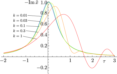
Figure 1: Absorption for different $k$ parameters

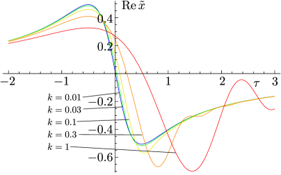
Figure 2: Dispersion for different $k$ parameters

4.3 Limiting Cases

For sufficiently slow sweep rates the envelope profile, Eq. 11, must approach the “static” resonance response, Eq. 4. We may show this to be so by expanding the error function in Eq. 11 in inverse powers of $\gamma$. In this way we find

$$\hat{x}\left({{\omega_{\mathrm{d}}}}\right)=\frac{Q}{{{\omega_{\mathrm{z}}}}}\frac{1}{{2Q\left({{\omega_{\mathrm{z}}}-{\omega_{\mathrm{d}}}}\right)+{\mathrm{i}}{\omega_{\mathrm{z}}}}}\left\{{1+\frac{{\mathrm{i}}}{{2{\gamma^{2}}}}-\frac{3}{{4{\gamma^{4}}}}-\frac{{15{\mathrm{i}}}}{{8{\gamma^{6}}}}+}\right.\dots$$ (12)

The pre-factor is the static response function and the series then shows how, with a finite sweep rate, the response evolves from this.

For the purposes of comparison it is expedient to normalize the response so that the absorption peak (in the quasi-static limit) has unit magnitude. Thus we define $\tilde{x}\left(\tau\right)$:

$$\tilde{x}\left(\tau\right)={{\hat{x}\left(\tau\right)}\mathord{\left/{\vphantom{{\hat{x}\left(\tau\right)}{\hat{x}\left({t=0,\;k\to 0}\right)}}}\right.\kern-1.2pt}{\left|\hat{x}\left({t=0,\;k\to 0}\right)\right|}}$$

so that

$$\tilde{x}\left(\tau\right)=\frac{{\left({1-{\mathrm{i}}}\right)}}{4}\sqrt{\frac{{2\pi}}{k}}\,{e^{{\mathrm{i}}{\gamma^{2}}}}{\mathop{\mathrm{Erfc}}\nolimits}\left[{\sqrt{\mathrm{i}}\,\gamma}\right]$$

In Figs. 1 and 2 we show the absorptive and dispersive parts of the response for different $k$ values. For the slowest sweep rate the response is indistinguishable from that of the quasi-static case. The first effect of a finite sweep rate is a small skewing of the resonance with a consequent delay in the occurrence of the resonance peak. Next there is a reduction of the peak height. Then for even faster sweep rates the resonance suffers significant distortion – particularly after the peak, where the absorption can become negative. Ultimately this evolves into no response before the resonance, and ringing after. This is indicated in Fig. 3. The ringing will decay with characteristic time $\tau_{\mathrm{d}}$. This may be seen by expanding $\tilde{x}\left(\tau\right)$ in powers of $\gamma$:

$$\tilde{x}\left(\tau\right)\sim\frac{1-\mathrm{i}}{4}\sqrt{\frac{2\pi}{k}}e^{{\mathrm{i}/4k}}e^{-\tau/k}e^{-\mathrm{i}\tau^{2}/k}\left\{1+\mathrm{O}\left(\frac{1}{\sqrt{k}}\right)\right\}.$$

The first exponential gives a simple phase factor. The second exponential gives the decay; in proper variables this is $e^{-t/\tau_{\mathrm{d}}}$. And the third exponential, in proper variables $e^{-\mathrm{i}\alpha t^{2}/2}$, gives the ringing at the “instantaneous” frequency deviation from $\omega_{\mathrm{z}}$.

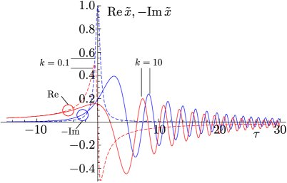
Figure 3: Absorption and dispersion for a rapid (solid lines) and a slow (dashed lines) frequency sweep

4.4 Comments on previous treatments

Our solution is a function of the reduced time $\tau$ (Eq. 10). This involves the product of time $t$ and sweep rate $\alpha$, so reversing $t$ is equivalent to reversing $\alpha$. Thus a down sweep will have a response that is the mirror image of an up sweep – as expected on intuitive grounds. However Cronin [8] found, in his series approximations, that the mathematical forms of the up and down sweeps were not identical. This disagreement can be traced back to our high-Q condition: specifically the discarding of the negative-frequency resonance. When this is not discarded it follows that the observed resonance profile will depend upon whether the “other” resonance has been passed through or not. Of course this difference will be numerically negligible in the high-Q case. One should also note that any realistic spectral sweep would span frequencies in the vicinity of the resonance; experimentally the other resonance would never be covered.

Hok’s approach [3] involves taking an inverse Laplace transform. In a crucial step he discards as negligible a term (involving his $\gamma_{2}$). This is equivalent to our discarding of the negative frequency resonance.

5 Resonance shift

5.1 Introduction

Spectroscopy experiments often require the precise location of a resonance peak. Our results above indicate that sweeping the response up through the resonance at a finite rate will result in the peak occurring at a slightly higher frequency, while sweeping down will result in a slightly lower frequency. Thus, for example, Phillips and Gold [18] in studying the de Haas-van Alphen effect in lead appreciated the necessity for applying corrections for a finite sweep rate.

We shall discuss the shift in terms of the intensity of the resonance, the square magnitude response $\left|\tilde{x}(\tau)\right|^{2}$:

$$|\tilde{x}(\tau)|^{2}=\frac{\pi}{4k}{e^{-\frac{2\tau}{k}}\mathrm{Erfc}\left[\frac{(1-\mathrm{i})-2(1+\mathrm{i})\tau}{2\sqrt{2k}}\right]\mathrm{Erfc}\left[\frac{(1+\mathrm{i})-2(1-\mathrm{i})\tau}{2\sqrt{2k}}\right]}.$$ (13)

This is shown in Fig. 4. Series expansion of $\left|\tilde{x}(\tau)\right|^{2}$ shows how the intensity profile evolves from the quasi-static case.

$$\eqalign{{\left|{\tilde{x}\left(\tau\right)}\right|^{2}}&=\frac{1}{{1+4{\tau^{2}}}}+\frac{{16\tau}}{{{{\left({1+4{\tau^{2}}}\right)}^{3}}}}k-\frac{{4\left({5-152{\tau^{2}}+80{\tau^{4}}}\right)}}{{{{\left({1+4{\tau^{2}}}\right)}^{5}}}}{k^{2}}\\ &-\frac{{384\left({7\tau-104{\tau^{3}}+112{\tau^{5}}}\right)}}{{{{\left({1+4{\tau^{2}}}\right)}^{7}}}}{k^{3}}+\dots}$$ (14)

The first term is the quasi-static solution. The latter terms give the increasing distortion.

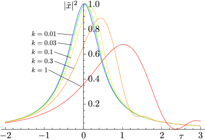
Figure 4: Variation of resonance intensity for different $k$ parameters

5.2 Frequency shift

The resonance peak corresponds to the maximum of the intensity. This peak evolves from the $\tau=0$ maximum as $k$ grows from zero. In order to find the position of the peak we must solve the equation

$$\frac{{{\mathrm{d}}{{\left|{\tilde{x}\left(\tau\right)}\right|}^{2}}}}{{{\mathrm{d}}\tau}}=0.$$ (15)

We do this in the following neat way. We expand the derivative of Eq. 14, $d={{{\mathrm{d}}{{\left|{\tilde{x}\left(\tau\right)}\right|}^{2}}}}/{{{\mathrm{d}}\tau}}$ as a power series in $\tau$:

$$\eqalign{d=&16\left({k-168{k^{3}}+720{k^{5}}+\dots}\right)\\ &-8\left({1-252{k^{2}}-5520{k^{4}}+100800{k^{6}}+\dots}\right)\tau\\ &-576\left({k-600{k^{3}}+1680{k^{5}}+\dots}\right){\tau^{2}}\\ &+64\left({1-1080{k^{2}}-31920{k^{4}}+403200{k^{6}}+\dots}\right){\tau^{3}}+\dots}$$

and we want to find the value of $\tau$ that will make this expression zero. We may revert this series, to give $\tau$ as a series in $d$. Then all we require is the leading term, corresponding to $d=0$. Thus we find the (reduced) time for the occurrence of the intensity peak, $\tau_{\mathrm{p}}$, as

$${\tau_{\mathrm{p}}}\left(k\right)=2k-56{k^{3}}+19104{k^{5}}-15194496{k^{7}}+\dots$$ (16)

This affirms that there is no shift when $k$ vanishes and it indicates how the shift evolves with $k$. However the successive coefficients of the series increase rapidly; this is a divergent series as indicated in Fig. 5, of use only for small $k$.

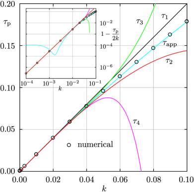
Figure 5: Shift of resonance frequency with increasing $k$ parameter. The black, red, green and purple lines show the successive Taylor approximants to the series, Eq. 16: truncated after the first, third, fifth and seventh powers.

The points in the figure are found directly from numerical solution of Eq. 15. The lines in the figure show successive Taylor approximants to the series.

It is clear that for small $k$ the leading-term linear behaviour is dominant. However the deviation from linearity is better-described, over a larger $k$ range, by a power series in $k^{1/2}$; this is shown by the cyan line in the figure, a least squares fit through the numerical points. Its equation is

$$\tau_{\mathrm{app}}\left(k\right)=2k+{b_{1}}{k^{{3\mathord{\left/{\vphantom{32}}\right.\kern-1.2pt}2}}}+{b_{2}}{k^{2}}+{b_{3}}{k^{{5\mathord{\left/{\vphantom{52}}\right.\kern-1.2pt}2}}}+{b_{4}}{k^{3}}$$ (17)

where

$$\eqalign{{b_{1}}&=-0.0334937425\\ {b_{2}}&=\phantom{-}1.6315734132\\ {b_{3}}&=-21.535018954\\ {b_{4}}&=\phantom{-}31.360499596\;.\\ }$$

This enables an accurate determination of the true resonance frequency $\omega_{\mathrm{z}}$ from the observed resonance frequency $\omega_{\mathrm{p}}$.

The inset to the figure, shows $1-\frac{\tau_{\mathrm{p}}}{2k}$ against $k$ with logarithmic axes. This indicates the limitation of the series approximation while demonstrating its merit of giving $\tau_{\mathrm{p}}$ with sufficient accuracy for larger values of $k$.

The reduced time of the peak $\tau_{\mathrm{p}}$ corresponds to a real time delay $t_{\mathrm{p}}$:

$$t_{\mathrm{p}}=\frac{\omega_{\mathrm{z}}}{\alpha Q}\tau_{\mathrm{p}}$$

so there is a frequency shift $\delta\omega$ of $\alpha t_{\mathrm{p}}$ or

$$\delta\omega=\frac{\omega_{\mathrm{z}}}{Q}\tau_{\mathrm{p}}\left(k\right).$$

For a slow sweep rate ($\alpha\ll\omega_{\mathrm{z}}^{2}/Q^{2}$), where we take only the leading term in the expansion: $\tau_{\mathrm{p}}=2k$, the time of the peak’s occurrence is

$$t_{\mathrm{p}}=2\tau_{\mathrm{d}}.$$

This is telling us that (in the slow-sweep limit) the resonance peak suffers a time delay of twice the oscillator’s ring-down time. This is intuitively reasonable, since $\tau_{\mathrm{d}}$ characterizes the time it takes for the oscillator to settle – the time it takes to respond to a stimulus. To this leading order of approximation we find the frequency shift of the peak to be

$$\delta\omega=2k\Delta\omega:$$ (18)

the resonance shift is $2k$ times the resonance width.

5.3 Peak attenuation

The normalized signal peak intensity and its evolution with increasing $k$ is found by substituting Eq. 16 into Eq. 14:

$$\left|{\tilde{x}\left({{\tau_{\mathrm{p}}}}\right)}\right|^{2}=1-4{k^{2}}+400{k^{4}}-152640{k^{6}}+\dots$$ (19)

The points in Fig. 6 are the peak intensities corresponding to different $k$ values, found directly from numerical solution of Eq. 15. The lines in the figure show the successive approximants to the series, Eq. 19. However the deviation from quadratic is better-described by a term in $k^{7/2}$; this is shown by the cyan line in the figure. Its equation is

$$\left|{\tilde{x}_{\mathrm{app}}\left({{\tau_{\mathrm{p}}}}\right)}\right|^{2}=1-4{k^{2}}+44{k^{7/2}}.$$

We note that the peak attenuation is a second-order effect; by contrast the frequency shift is a first-order effect.

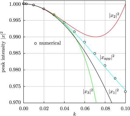
Figure 6: Reduction of peak intensity with increasing $k$ parameter. The black $(|x_{1}|^{2})$, red $(|x_{2}|^{2})$ and green $(|x_{3}|^{2})$ lines in the figure show the successive Taylor approximants to the series, Eq. 19: truncated after the first, third, fifth and seventh powers.

6 The parameter $k$

The fundamental equation of motion, Eq. 1 involves the quantities $\omega_{\mathrm{z}}$, $Q$ and $\alpha$. However, as we have seen from Eq. 11, in describing the shape of the resonance profile these quantities coalesce into the single dimensionless parameter $k$. We note, parenthetically, that this collapse cannot be demonstrated directly from the original equation of motion; it arises directly from the high-Q assumption, by which Eq. 11 follows from Eq. 6.

Within the framework of this approximation the absolute frequency of the oscillator, $\omega_{\mathrm{z}}$ disappears from consideration. We have the width of the resonance $\Delta\omega=\omega_{\mathrm{z}}/Q$ and the only other quantity in the equation of motion is the sweep rate $\alpha$, which has the dimensions of frequency squared. The dimensionless $k$ is simply the ratio $\alpha/2(\Delta\omega)^{2}$.

From the previous section we found, in the slow-sweep limit, that

$$k=\frac{\delta\omega}{2\Delta\omega};$$

$k$ is half the shift, expressed as a fraction of the width.

Yet another aspect of the meaning of $k$ will be seen in the next section, where we will find that it corresponds to the aspect ratio of the system’s Wigner distribution.

7 Wigner representation

The Wigner function attempts to describe how the frequency spectrum of a function – our $x(t)$ – varies with time. The Wigner distribution is defined as [12]

$$W\left({t,\omega}\right)=\frac{1}{{2\pi}}\int{{x^{*}}\left({t-{\tau\mathord{\left/{\vphantom{\tau 2}}\right.\kern-1.2pt}2}}\right){e^{-{\mathrm{i}}\omega\tau}}x\left({t+{\tau\mathord{\left/{\vphantom{\tau 2}}\right.\kern-1.2pt}2}}\right){\mathrm{d}}\tau}.$$

The interpretation of such a time-frequency distribution is that the integral

$$p=\int\limits_{{t_{1}}}^{{t_{2}}}{\int\limits_{{\omega_{1}}}^{{\omega_{2}}}{W\left({t,\omega}\right)}\,{\mathrm{d}}\omega\,{\mathrm{d}}t}$$ (20)

is proportional to the energy in the signal in the frequency range ${\omega_{1}}<\omega<{\omega_{2}}$ during the time interval ${t_{1}}<t<{t_{2}}$. The Uncertainly Principle implies that this result will be meaningless if the observed cell in time-frequency space is too small; in order for Eq. 20 to be meaningful we require

$$\left({{t_{2}}-{t_{1}}}\right)\left({{\omega_{2}}-{\omega_{1}}}\right)\gtrsim 1.$$

It follows from this that there is considerable latitude in the specification of a time-frequency distribution function; indeed, as Cohen has shown [19], the Wigner distribution is but one of a large class of possible time-frequency distributions. Galleani and Cohen evaluated exactly the Wigner distribution for the Gliding Tone problem [11]. They found:

$$W\left({t,\omega}\right)=\theta\left(\tau\right)\frac{{{e^{-{\omega_{\mathrm{z}}}\tau/Q}}}}{{2\alpha{\omega_{\mathrm{f}}}}}\left\{{\frac{{\sin 2\left({\omega-{\omega_{\mathrm{f}}}}\right)\tau}}{{\omega\left({\omega-{\omega_{\mathrm{f}}}}\right)}}-\frac{{\sin 2\left({\omega+{\omega_{\mathrm{f}}}}\right)\tau}}{{\omega\left({\omega+{\omega_{\mathrm{f}}}}\right)}}}\right\}$$

where

$$\tau=t-{\omega\mathord{\left/{\vphantom{\omega\alpha}}\right.\kern-1.2pt}\alpha}$$

and $\omega_{\mathrm{f}}$ is defined in Eq. 3. A typical density plot is shown in Fig. 7.

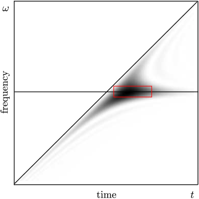
Figure 7: Wigner distribution density for Gliding Tone problem. The horizontal line indicates the natural resonance of the oscillator $\omega_{\mathrm{z}}$ and the sloping line represents the increase of drive frequency with time ${\omega}={\omega_{\mathrm{z}}}+\alpha t$. The significance of the rectangular box is discussed around Eq. 21.

The horizontal line indicates the natural resonance of the oscillator $\omega_{\mathrm{z}}$ and the sloping line represents the increase of drive frequency with time $\omega={\omega_{\mathrm{z}}}+\alpha t$. The Wigner distribution function indicates that the response is concentrated close to the intersection of these lines – where the excitation is in the vicinity of the natural resonance. The density along the sloping line shows the response at the excitation frequency. The density along the horizontal line shows the “ringing” at the oscillator’s natural frequency caused by the “shock” of the excitation frequency varying. The response being all to the right of the sloping line is a manifestation of causality.

The height of the distribution, the extension in frequency, is the breadth of the resonance, $\omega_{\mathrm{z}}/Q$. The width of the distribution, the extension in time, is the ring-down time ${\tau_{\mathrm{d}}}=2{Q\mathord{\left/{\vphantom{Q{{\omega_{\mathrm{z}}}}}}\right.\kern-1.2pt}{{\omega_{\mathrm{z}}}}}$. This translates to a frequency sweep width of $2{{\alpha Q}\mathord{\left/{\vphantom{{\alpha Q}{{\omega_{\mathrm{z}}}}}}\right.\kern-1.2pt}{{\omega_{\mathrm{z}}}}}$. And the ratio of these frequencies is $2\alpha{\left({{Q\mathord{\left/{\vphantom{Q{{\omega_{\mathrm{z}}}}}}\right.\kern-1.2pt}{{\omega_{\mathrm{z}}}}}}\right)^{2}}$; this is precisely Barber and Ursell’s $k$ parameter [4], Eq. 9. Thus $k$ determines the aspect ratio of the Wigner distribution:

$$k=\frac{{{\mathrm{extension~{}in~{}time~{}space}}}}{{{\mathrm{extension~{}in~{}frequency~{}space}}}},$$ (21)

with both measured in the same units. A box of the appropriate aspect ratio is shown in Fig. 7. Observe that it does suggest the aspect ratio of the Wigner density.

The above result also indicates the possibility that the Wigner distribution may be expressible in universal form. In order to demonstrate this universality we take the Wigner distribution as

$$W\left({t,\omega}\right)=\frac{1}{{2\alpha{\omega_{\mathrm{f}}}}}\theta\left(\tau\right){e^{-{{{\omega_{\mathrm{z}}}\tau}\mathord{\left/{\vphantom{{{\omega_{\mathrm{z}}}\tau}Q}}\right.\kern-1.2pt}Q}}}\frac{{\sin 2\left({\omega-{\omega_{\mathrm{f}}}}\right)\tau}}{{\omega\left({\omega-{\omega_{\mathrm{f}}}}\right)}}$$

where we have used the high-Q procedure of discarding the negative frequency resonance. We first apply a horizontal shear to this function so that $\tau=t-\omega/\alpha$ becomes the independent “time” variable; the sloping line of Fig. 7 becomes the vertical axis. And then we scale the time and frequency variables to the dimensionless

$$\Omega=\omega\sqrt{{k\mathord{\left/{\vphantom{k\alpha}}\right.\kern-1.2pt}\alpha}},\;\;\;\;\;\;T=\tau\sqrt{{\alpha\mathord{\left/{\vphantom{\alpha k}}\right.\kern-1.2pt}k}}.$$

We also need the auxiliary ${\Omega_{\mathrm{f}}}={\omega_{\mathrm{f}}}\sqrt{{k\mathord{\left/{\vphantom{k\alpha}}\right.\kern-1.2pt}\alpha}}$. In terms of these variables the Wigner distribution function is

$$W\left({T,\Omega}\right)=\frac{{\sqrt{k}}}{{2{\alpha^{{3\mathord{\left/{\vphantom{32}}\right.\kern-1.2pt}2}}}{\omega_{\mathrm{f}}}\omega}}\theta\left(T\right){e^{-\sqrt{2}T}}\frac{{\sin\left({\Omega-{\Omega_{\mathrm{f}}}}\right)T}}{{\left({\Omega-{\Omega_{\mathrm{f}}}}\right)}}.$$

In the spirit of the high-Q approximation we argue that $W\left({T,\Omega}\right)$ is non-zero only in the vicinity of $\omega\sim{\omega_{\mathrm{f}}}$, and we thus write

$$W\left({T,\Omega}\right)=\frac{{\sqrt{k}}}{{2{\alpha^{{3\mathord{\left/{\vphantom{32}}\right.\kern-1.2pt}2}}}\omega_{\mathrm{f}}^{2}}}\theta\left(T\right){e^{-\sqrt{2}T}}\frac{{\sin\left({\Omega-{\Omega_{\mathrm{f}}}}\right)T}}{{\left({\Omega-{\Omega_{\mathrm{f}}}}\right)}}.$$

There is a system-dependent pre-factor but the time and frequency dependence are all in the dimensionless variables.

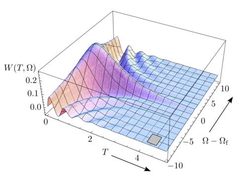
Figure 8: Wigner distribution in terms of reduced variables

This is plotted in Fig. 9. The oscillations (and in particular the fact that $W\left(T,\Omega\right)$ goes negative) are an artefact of the Wigner distribution; it is only the integral over an “uncertainty” area that is meaningful as a (necessarily non-negative) probability. We show, in the figure, the grey rectangle indicating the scale of this region.

8 Complex plots

A convenient graphical representation of a system’s response is provided by plotting the imaginary part against the real part of the complex response function, sometimes referred to as a hodograph. In the context of an oscillator the parametric plot is mapped out as as one sweeps through the resonance, the applied frequency being the variable parameter of the plot. In comparison with separate plots of the real and imaginary parts of the response versus excitation frequency, the complex plot involves a loss of information: frequency is no longer an explicit variable. However this can an advantage. In general the response function of a system will be complicated. In its mathematical description the dependence on frequency typically will be as a product $\omega\tau_{\mathrm{c}}$, where $\tau_{\mathrm{c}}$ is a characteristic time. It is then equally valid to regard $\omega\tau_{\mathrm{c}}$ as the parameter of the plot. The actual frequency and characteristic time are not important; it is only their product. Thus the parametric plot is able to demonstrate generic properties of the response function. Indeed one might also measure the response at constant applied frequency while varying $\tau_{\mathrm{c}}$, perhaps indirectly by changing the temperature or pressure.

The complex plot of the quasi-static or normal Lorentzian resonance has a circular locus. Distortion of the resonance, as follows from the Gliding Tone effect, manifests itself as a deviation from circularity. Some examples are shown in Fig. 9 (where the curves are traversed in the anti-clockwise sense). The distortion worsens with increasing $k$ parameter, as one would expect. There are three effects to note: i) before resonance the magnitude response (the radius vector) is smaller than the quasistatic value; ii) on passing the resonance the response will become greater, leading, for large $k$ to iii) ringing.

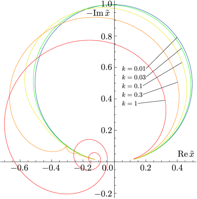
Figure 9: Complex plot of oscillator response for different $k$ parameters

9 Experimental measurements

The motivation for the above study has been the interpretation and understanding of our experiments on the putative supersolid phase of helium. Torsional oscillators of high Q-factor provide sensitive sensors of “lost mass” through its reflection in small changes of resonance frequency. Indeed such an oscillator was used in the discovery that the superfluid transition in two-dimensional liquid ⁴He was of the Kosterlitz-Thouless type [20].

We now show some measurements performed in our laboratory, on torsional oscillators as typically used in low-temperature physics research [21]. The oscillator – particularly the torsion rod – is made of coin silver, and carefully annealed to increase its Q-factor. The oscillator is driven and the response detected both electrostatically. Our measurements were made at low temperatures, where $Q$s of order $10^{6}$ are achievable.

A first example is given in Fig. 10. The plots show sweeps up and down through the resonance and the displacement of the peaks indicates that there is an effect which must be addressed in order to draw correct inferences from frequency measurements. The frequency was swept at $7.3\times 10^{-5}\mathrm{Hz\hskip 2.0pts^{-1}}$ up and down through the resonance at $418.343510\,\mathrm{Hz}$, the oscillator having a Q-factor of 24,750. According to Eq. 9 this gives a $k$ parameter of 0.081, implying a peak’s (dimensionless) time shift $\tau=0.149$ which from Eq. 18, corresponding to a frequency shift of 2.52 mHz. The bar in the inset shows the expected separation of 5.04 mHz between the experimental peaks.

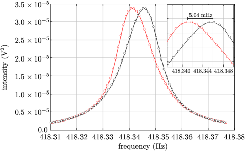
Figure 10: Distortion of resonance caused by a finite sweep rate corresponding to a $k$ parameter of 0.081. Black: up sweep, Red: down sweep.

The hodograph corresponding to this plot (the up sweep only) is shown in Fig. 11. It is salutary to note that while either single sweep of Fig. 10 might not be recognized as embodying a measure of distortion – indeed a Lorentzian fit through the data may be misleadingly good – it is the complex plot that gives the clearest indication of resonance distortion.

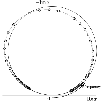
Figure 11: Distortion of complex plot caused by a finite sweep rate corresponding to a $k$ parameter of 0.081. For comparison the corresponding quasi-static circular profile is shown.

Finally, in Fig. 12 we show a sequence of spectra, taken with different sweep rates. The quasi-static resonance frequency is 396.1824 Hz. This is shown in the figure and already the slowest curve ($k=0.0625$) shows a discernible shift. As $k$ increases we see evolution of the characteristic features: i) shift of the peak frequency, ii) reduction in the peak height, iii) increasing asymmetry of the curve, and iv) the emergence of ringing at the fastest sweep. The lines in the figure are calculated from Eq. 11. The agreement is gratifying.

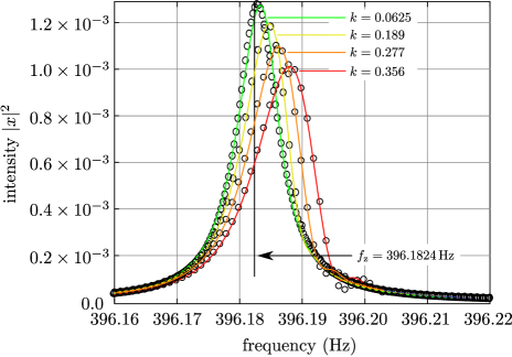
Figure 12: Resonance intensity for a range of $k$ values

10 Conclusion

The solution to the Gliding Tone problem has been obtained in closed form in terms of known functions. The sole non-exact feature is that the Q-factor of the oscillator is assumed to be high. In the high-Q case the variables of the problem combine into a single parameter ($\gamma$), in terms of which the solution is expressed. We investigated the deviation from the quasi-static oscillator response as a consequence of the finite sweep rate, showing that the resonance distortion depended on the dimensionless parameter $k$. To lowest order the delay in the appearance of the resonance peak corresponds to double the oscillator’s ring-down time. Experimental observations on a high-Q torsional oscillator are shown to be consistent with the theory presented.

11 Acknowledgements

We thank Dr. Jan Nyèki for raising this problem and Prof. Leon Cohen for expressing encouraging interest in the work and for providing some helpful contextual comments. Prof. Lorenzo Galleani was kind enough to clarify the form of the Gliding Tone Wigner distribution. We are grateful to Prof. Nico Temmi for advice on the nomenclature and properties of the “error-related” functions.

We used the Mathematica software package for performing many of the algebraic manipulations; we note, in particular, that the mathematical steps in arriving at Eq. 16 were exceedingly labour-intensive as sufficient terms in the intermediate series must be taken in order for the contributions to each power of $k$ to be exhausted. It took 8.5 hours on a fairly standard PC to obtain terms up to $k^{7}$ and 128 hours for the next term!

12 References

References

- [1] F. M. Lewis, Vibration During Acceleration Through a Critical Speed, Trans. Am. Soc. Mech. Eng., 54, 253-261 (1932)
- [2] J. G. Baker, Mathematical-Machine Determination of the Vibration of Accelerated Unbalanced Rotor, Journal of Applied Mechanics - Trans. A.S.M.E. 61, A145-A160 (1939)
- [3] G. Hok, J. App. Phys. 19, 242-250 (1948)
- [4] N. F. Barber and F. Ursell, The Response of a Resonant System to a Gliding Tone, Phil. Mag. 39, 345-361 (1948)
- [5] G. D. McCann and R. R. Bennett, Vibration of Multi-frequency Systems During Acceleration Through Critical Speeds, J. App. Mech., 16 375-382 (1949)
- [6] D. Macchia, Acceleration of an Unbalanced Rotor Through the Critical Speed, Am. Soc. Mech. Eng., Winter Meeting, 2-7 (1963) – and MSc Thesis
- [7] E. L. R. Corliss, Resolution Limits of Analyzers and Oscillatory Systems, J. Res. NBS 67A, 461-474 (1963)
- [8] D. L. Cronin, Response of Linear, Viscous Damped Systems to Excitations having Time-Varying Frequency, Ph. D Thesis, California Institute of Technology (1965)
- [9] A. B. Pippard, The Physics of Vibration, Cambridge, (1989)
- [10] D. Schoenberg, Phil. Trans. Roy. Soc. London, A255, 85-133 (1962)
- [11] L. Galleani and L. Cohen, On the Exact Solution to the “Gliding Tone Problem” IEEE SSAP 2000, Pocono Manor, Pennsylvania, USA, August (2000)
- [12] E. Wigner, On the Quantum Correction For Thermodynamic Equilibrium, Phys. Rev. 40, 749-759 (1932)
- [13] M. Abramowitz and I. A. Stegun, Handbook of Mathematical Functions, National Bureau of Standards, New York, (1964)
- [14] Frank W. J. Olver, Daniel W. Lozier, Ronald F. Boisvert and Charles W. Clark, NIST Handbook of Mathematical Functions, Cambridge University Press, Cambridge, (2010)
- [15] Burton D. Fried and Samuel D. Conte, The Plasma Dispersion Function – the Hilbert Transform of the Gaussian, Academic Press, New York, (1961)
- [16] A. B. Mikhailovsky, Theory of Plasma Instabilities, Atomizdat, (1975) (in Russian)
- [17] V. N. Fadeeva and N. M. Terent’ev, Tables of Values of the Probability Integral for Complex Arguments, State Publishing House for Technical Theoretical Literature, Moscow, (1954)
- [18] R. A. Phillips and A. V. Gold, Landau-Level Widths, Effective Masses, and Magnetic Interaction Effects in Lead, Phys. Rev. 178, 932 (1969)
- [19] L. Cohen, Time-Frequency Analysis, Prentice-Hall, Englewood Cliffs, NJ, USA, (1995)
- [20] D. J. Bishop and J. D. Reppy, Phys. Rev. Lett., 40, 1727-1730 (1978)
- [21] R. C. Richardson and E. N. Smith (Eds), Experimental Techniques in Condensed Matter Physics at Low Temperatures, Addison-Wesley, (1998)