CO in the C1 globule of the Helix nebula with ALMA

Abstract

We present and analyse ¹²CO, ¹³CO and C¹⁸O(2–1) ALMA observations of the C1 globule inside the Helix nebula in order to determine its physical properties. Our findings confirm the molecular nature of the globule with a multi-peak structure. The ¹²CO line has a high optical depth $\tau\sim$10. The derived ¹²C/¹³C$\sim$10 and ¹⁶O/¹⁸O$\sim$115 ratios are not in agreement with the expected isotopic ratios of carbon-rich AGB stars. Assuming that the ¹²CO optical depth has been underestimated, we can find a consistent fit for an initial mass of 2 M_⊙. We obtain a molecular mass of $\sim$2$\,\times 10^{-4}\,$$\textup{M}_{\odot}$ for the C1 globule, which is much higher than its mass in the literature. Clumping could play a role in the high molecular mass of the knot. The origin of the tail is discussed. Our findings show that the most probable model appears to be shadowing. The kinematics and molecular morphology of the knot are not consistent with a wind-swept model and the photoevaporation model alone is not enough to explain the nature of the globule. We propose an integrated model where the effects of the photoevaporation, the stream and shadowing models are all considered in the tail shaping process.

1 Introduction

The Helix nebula (NGC 7293) is one of the closest known planetary nebulae (PN) at a distance of 201$\pm 4$ pc (Gaia Collaboration, 2018). One of the most interesting characteristics of the Helix nebula is the presence of microstructures known as cometary knots inside its molecular envelope (e.g. Huggins et al. 1996). Those knots, first reported by Vorontsov-Velyaminov (1968), are dense clumps of gas and dust. They exhibit a crescent-shaped head in optical images (e.g. O’Dell et al. 2002, Meaburn et al. 1992) and may possess a tail pointing away from the central star (CS). In this paper, the terms cometary knots, knots and globules are interchangeable and do not distinguish whether the knots present a defined tail or not.
Globules are thought to be common structures inside PNe, especially in those with a molecular envelope (Huggins et al., 1996) such as the Ring and the Dumbbell nebulae (O’Dell et al., 2002). With a typical size of around $10^{13}$m (e.g. Nishiyama 2018), the knots in the Helix nebula can be resolved and studied in detail due to its proximity. Matsuura et al. (2009) estimated the number of globules in the Helix nebula to be around $40\,000$, with different distributions for globules located closer to the CS, which are more or less isolated, and those far from the CS, which are more overlapping in images.

Understanding the nature and behaviour of the knots is of great importance to understand the physical processes reigning inside the planetary nebula host. Over the past years, optical analyses have permitted the estimation of properties such as the kinematics, the morphology and the lifespan of the knots (e.g. Meaburn et al. 1998, 1996, 1992). Studies have also been conducted in H₂ (e.g. Matsuura et al. 2009) and CO (Huggins et al. 1992, Young et al. 1997) to derive the molecular characteristics, such as the mass, the number and the density of systems of knots as well as of individual globules such as the C1 globule (Huggins et al., 2002). One of the biggest uncertainties on the knots is their formation and evolution. Though a number of models have been suggested to explain how they formed (e.g. Dyson et al. 2006, López-Martín et al. 2001, Cantó et al. 1998), whether they have been created during or after the AGB phase and how they obtained their comet-like shape remains unclear.

The aim of this paper is to determine the physical properties of the globules in the Helix nebula by investigating the CO emission from an individual knot: the C1 globule. C1 is a near-side globule located at $+\,136^{\prime\prime}$ North to the CS (Huggins et al., 1992). We report and analyse new CO data of the knot with significantly better resolution than previous observations.
This paper is organized as follows. In Section 2, we present the ALMA data used in this work and describe the data reduction process. Our results are presented in Section 3, in which the line intensities, the morphology and the optical depth are discussed. The following sections discuss the isotopic ratios, the molecular mass, the dust emission and the origin of the globules. Section 7 closes the paper with a conclusion.

2 Data and data reduction

The data used in this analysis were obtained from the ALMA archive under the project code 2012.1.00116.S. The C1 globule was observed with 40 12-m ALMA dishes at band 6 between 2014 July 21 and 27 (PI: Huggins), with a maximum baseline of 820.2m. The observations covered a field of view of $\sim$28 arcsec with an angular resolution of $0.39\,$arcsec and a total integration time of $2.9\,$h. The C1 globule in the Helix nebula is located at a right ascension of $22$h $29$m $37.833$s and a declination of $-20^{\circ}$ $47^{\prime}$ $55.017^{\prime\prime}$ (J2000).

We manually calibrated the data using casa (McMullin et al., 2007). The retrieved data consist of four different measurement sets which we calibrated independently.
For each measurement set, we initially performed calibration of the system temperature of the antennas and atmospheric water vapour. The complete measurement sets have twenty-four spectral windows from which were extracted the spectral windows centred on $230.573$, $220.432$ and $219.596$ GHz, corresponding to ¹²CO(2–1), ¹³CO(2–1) and C¹⁸O(2–1), respectively, and on $231.635\,$GHz for the continuum emission. Each spectral line window has a width of $117.187\,$MHz over $3\,840$ channels with a velocity resolution of $0.05\,$km s^-1, whereas the continuum window covers a 1.875 GHz width with 128 channels.
The data were flagged to exclude shadowed antennas and end channels with poor receiver response. The data were then calibrated for bandpass, flux scaling, amplitude and phase of the complex visibilities using standard CASA procedures. The calibrators used were the quasar J2258-279 and the Seyfert galaxy J2258-2758 which were used as flux and bandpass/phase calibrators, respectively.
The calibrated data from the four individual sets were then combined into one calibrated measurement set.

After calibration, spectral cubes were extracted for each molecular line across all channels using the multiscale deconvolution algorithm, along with a continuum map obtained with the Högbom algorithm of the casa imaging task tclean. The chosen size of a pixel is $0.07\,\textmd{arcsec}$ and Briggs weighting was applied to all images with $robust\,$=$\,0.5$. The resultant data cubes have beam sizes of $0.41\times 0.35$, $0.42\times 0.36$ and $0.43\times 0.36$ $\textmd{arcsec}\,\times\,\textmd{arcsec}$, and typical rms noises ($\sigma_{12}$, $\sigma_{13}$, $\sigma_{18}$) of $3.5$, $2.6$ and $2\,\textmd{mJy}\,\textmd{beam}^{-1}$ for ¹²CO, ¹³CO and C¹⁸O, respectively. The size of the synthesised beam for the continuum map is $0.40\times 0.34$ in arcsec, with an rms noise of $\sim 20\,\mu\textmd{Jy}\,\textmd{beam}^{-1}$. Continuum subtraction was not applied when producing the line cubes as the continuum emission is weak. For creating ratio maps, all images were created at the resolution of the ¹³CO map.

3 Results

3.1 Morphology

CO emission in the cometary knots of the Helix nebula was first detected by Huggins et al. (1992). The molecular nature of the knots was then supported by the findings of Huggins et al. (2002) who imaged the C1 globule in CO(1–0) with a velocity resolution of $0.2\,\textmd{km}\,\textmd{s}^{-1}$ and a spatial resolution of 3.6 arcsec. With a velocity resolution of $0.05\,\textmd{km}\,\textmd{s}^{-1}$ and an angular resolution of $0.39\,$arcsec, our data enables us to closely observe the molecular distribution of the C1 globule.
The integrated intensities of the ¹²CO and ¹³CO line emissions shown in Fig. 1 confirm that the C1 knot is molecular, with strong emission from the head of the knot as well as from its extended tail. The structure of the globule is not well defined in the C¹⁸O integrated intensity map as the emission is weak.

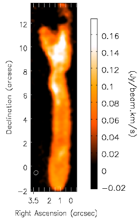
(a) (b)

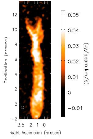
(c)

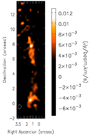
Figure 1: CO integrated intensity maps of the C1 globule. The elliptical restoring beams (in arcsec $\times$ arcsec) are located at the bottom left of each map. (a): ¹²CO with beam size $0.41\times 0.35$, (b):¹³CO with beam size $0.42\times 0.36$ and (c): C¹⁸O with beam size $0.43\times 0.36$.

The molecular head of the globule is ellipsoidal and is $\sim 1^{\prime\prime}$ offset to the crescent-shaped ionized head observed in the optical (e.g. O’Dell & Handron 1996) as shown in Fig. 2. The tail is pointing away from the central star with a roughly cylindrical shape. We define the tail as the region of the knot starting at $\sim 2^{\prime\prime}$ away from the tip of the head of the globule in CO.

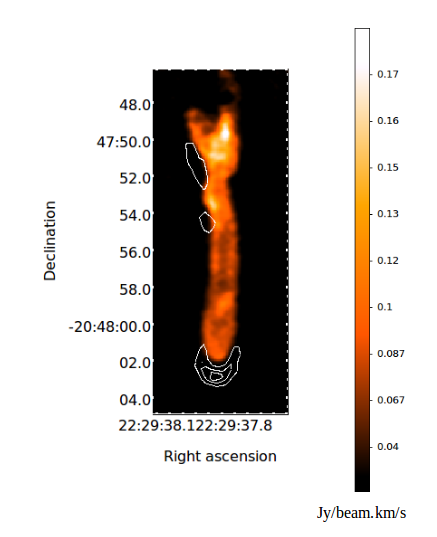
Figure 2: ¹²CO integrated intensity map overlaid with HST H$\alpha\,$+[N ii] contour map. The contours levels are at $0.76$, $1.53$, $2.31$ and $3.08$ in $10^{-22}\,\textmd{erg}\,\textmd{cm}^{-2}\,\textmd{s}^{-1}\,$Å^-1. The molecular head is $\sim 1^{\prime\prime}$ offset to the crescent-shaped head observed in the optical.

We notice the presence of peak intensities at different positions in the knot in the ¹²CO and ¹³CO maps (Fig. 1). Some of the peaks are located close to the head, but peaks are also observed in the body, and strong emission is emitted in the tail region. At each peak, the direction of the tail seems to slightly deviate. This phenomenon is known as tail meandering. Matsuura et al. (2009) reported that globules can present one or multiple peaks where a change of the direction of the tail can occur, which is in agreement with our observations.
We find that the peak intensity of the emission seems to be higher in the tail than in the head of the knot. This is in contrast with the result of Matsuura et al. (2007) who observed that the peak intensity decreases by a factor of 10 between the head and the tail in H₂. In addition, Matsuura et al. (2009) noticed the existence of brightness gaps at the midpoint along the tail in different knots, which are also visible in our ¹²CO data, at $\sim+$0.5, $+\,$2.5 and $+\,5^{\prime\prime}$ (Fig. 1). In ¹³CO, the gap is observed in the head of the globule.

3.2 Line intensity

The integrated ¹²CO, ¹³CO and C¹⁸O spectra and their respective Gaussian fittings are shown in Fig. 3. The ¹²CO line emission has a peak intensity of 16.1 Jy, and a full width at half maximum (FWHM) of 0.81$\,\textmd{km}\,\textmd{s}^{-1}$. The ¹³CO line peaks at 5.5 Jy, with a FWHM of 0.56$\,\textmd{km}\,\textmd{s}^{-1}$. The C¹⁸O spectral profile presents a peak value of 0.36 Jy and a FWHM of 0.41$\,\textmd{km}\,\textmd{s}^{-1}$. The ¹²CO emission has a total flux of 14.4$\,\textmd{Jy}\,\textmd{km}\,\textmd{s}^{-1}$. The total ¹³CO and C¹⁸O fluxes are 3.5 and 0.18$\,\textmd{Jy}\,\textmd{km}\,\textmd{s}^{-1}$, respectively.

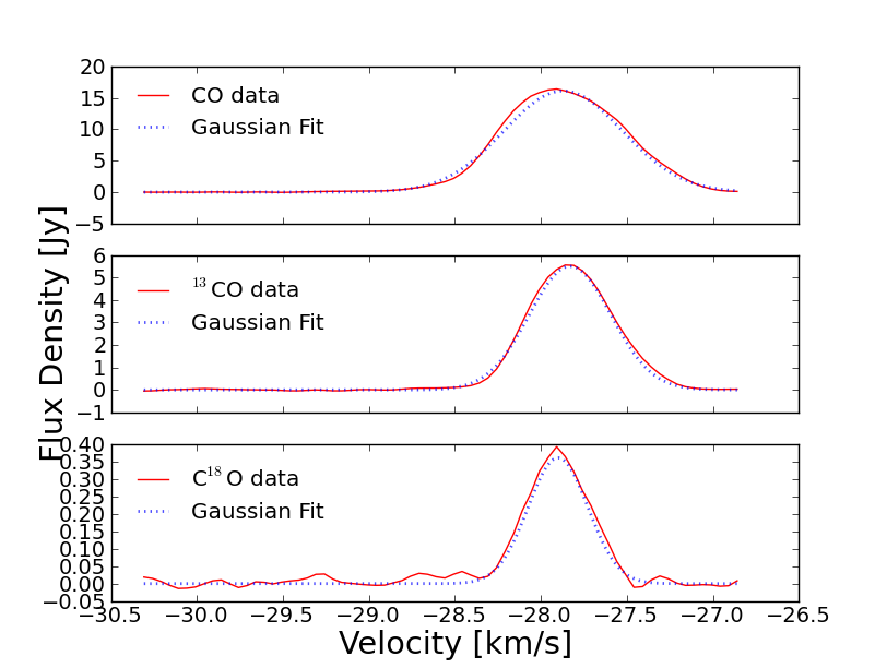
Figure 3: Spectral profiles of the CO(2–1) lines with corresponding Gaussian fittings. The ¹²CO (top) Gaussian line is centred at $-27.87\,\textmd{km}\,\textmd{s}^{-1}$ with a peak intensity of $16.1\,\textmd{Jy}$ and a FWHM of $0.81\,\textmd{km}\,\textmd{s}^{-1}$. ¹³CO (middle), centred at $-27.83\,\textmd{km}\,\textmd{s}^{-1}$ with a peak intensity of $5.5\,\textmd{Jy}$, has a FWHM of $0.56\,\textmd{km}\,\textmd{s}^{-1}$. (bottom) shows the C¹⁸O spectral profile centred at $-27.91\,\textmd{km}\,\textmd{s}^{-1}$ with a peak value of $0.36\,\textmd{Jy}$ and a FWHM of $0.41\,\textmd{km}\,\textmd{s}^{-1}$.

3.3 Optical depth

Under the assumption of Local Thermodynamic Equilibrium (LTE), and assuming that ¹²CO, ¹³CO and C¹⁸O have the same excitation temperature T${}_{\textmd{ex}}$ and that ¹²CO is optically thick, we derive T${}_{\textmd{ex}}$ from the ¹²CO line using

$$T_{\textmd{ex}}=11.06\,\Bigg{\{}\textmd{ln}\,\bigg{[}1+\frac{11.06}{T_{\textmd{peak}}^{12,2-1}+0.19}\bigg{]}\Bigg{\}}^{-1}\,\textmd{K}$$ (1)

(e.g. Nishimura et al. 2015) where ${T_{\textmd{peak}}^{12,2-1}}=24.96\,\textmd{K}$ is the peak intensity of the ¹²CO(2–1) emission. We find $T_{\textmd{ex}}=\,30\,\textmd{K}$. Masks were applied to the ¹³CO and C¹⁸O integrated intensity maps in order to pick only the emission from the real source and avoid background noise, with cut-offs at $3\sigma_{13}$ and $2\sigma_{18}$ for ¹³CO and C¹⁸O, respectively. The optical depths of ¹³CO and C¹⁸O, $\tau_{13}$ and $\tau_{18}$, are given by (e.g. Nishimura et al., 2015)

$$\tau_{13}=-\textmd{ln}\Bigg{\{}1-\frac{T_{\textmd{mb}}^{13,2-1}(v)}{10.58}\Bigg{[}\frac{1}{\textmd{exp(10.58/$T_{\textmd{ex}}$)-1}}-0.02\Bigg{]}^{-1}\Bigg{\}}$$ (2)

$$\tau_{18}=-\textmd{ln}\Bigg{\{}1-\frac{T_{\textmd{mb}}^{18,2-1}(v)}{10.54}\Bigg{[}\frac{1}{\textmd{exp(10.54/$T_{\textmd{ex}}$)-1}}-0.02\Bigg{]}^{-1}\Bigg{\}}\,\textmd{,}$$

where $T_{\textmd{mb}}$ is the line temperature at a specific velocity $v$. Using the Rayleigh-Jeans law, the maps in units of intensity are converted to maps in units of brightness temperature with (e.g. Thompson et al., 1986)

$$T_{\textmd{mb}}=1.222\times 10^{3}\frac{I}{\nu^{2}\,\theta_{\textmd{maj}}\,\theta_{\textmd{min}}}\,\textmd{K}\,\textmd{,}$$ (3)

where $I$ is the intensity in mJy beam^-1, $\nu$ is the frequency in GHz. $\theta_{\textmd{maj}}$ and $\theta_{\textmd{min}}$ are the major and minor axes of the synthesised Gaussian beam. For the ¹³CO map, $\theta_{\textmd{maj}}=0.42\,$arcsec and $\theta_{\textmd{min}}=0.36\,$arcsec, whilst for the C¹⁸O map $\theta_{\textmd{maj}}=0.43\,$arcsec and $\theta_{\textmd{min}}=0.36\,$arcsec.
We find a maximum optical depth of $0.99$ and $0.16$ for ¹³CO and C¹⁸O, respectively. Using the observed ¹²CO/¹³CO ratio of $\sim$10 found by Bachiller et al. (1997) for the entire nebula, we estimate the ¹²CO optical depth to be up to $\sim$10. Huggins et al. (1992) assumed that ¹²CO in the C1 globule is optically thin. With the higher resolution achieved by ALMA, we find that ¹³CO is mostly optically thin and C¹⁸O is always optically thin, while the ¹²CO emission is highly optically thick.
Figure 4 shows the $\tau_{13}$ map integrated over all the channels, as well as the ¹³CO optical depth channel maps of the C1 globule. Assuming the previously mentioned ¹²CO and ¹³CO ratio of $\sim\,$10, we look for optically thin ¹²CO regions where $\tau_{13}<0.1$.
We observe that the optical depth is not the same along the knot. The integrated optical depth map (Fig. 4a) shows that the inner region of the globule is optically thick in ¹²CO, and the highest optical depths are located at declinations from $+0\textmd{ to}+3^{\prime\prime}$ and $+\,6\textmd{ to}+10^{\prime\prime}$. The extended tail (at declination $>+10^{\prime\prime}$) shows the lowest optical depth in ¹³CO ($\sim$0.1). The channel maps show how the ¹³CO optical depth varies along the globule at different velocities. In Fig. 4b and 4c, the tail presents high optical depth, whereas the head appears less optically thick. The region at declinations between $+1^{\prime\prime}$ and $+4^{\prime\prime}$ is always optically thick. In the tail region, the ¹³CO optical depth reaches up to $0.9$ at a velocity of $-27.65\,\textmd{km}\,\textmd{s}^{-1}$ and a declination of $\sim+6^{\prime\prime}$ (Fig. 4c). In Fig. 4d, the entire inner part of the body is optically thick. The maximum optical depth $\tau_{13\textmd{max}}=0.99$ is observed close to the head at a declination of $+1.7^{\prime\prime}$ and at a velocity of $-27.90\,\textmd{km}\,\textmd{s}^{-1}$ (Fig. 4e). The head of the globule is optically thick in Fig. 4f while the higher part of the tail seems to be optically thin. In Fig. 4g, a relatively high optical depth value is observed at a declination of $+6^{\prime\prime}$, which could potentially represent a separate knot. This feature is observed from Fig. 4f to Fig. 4i.

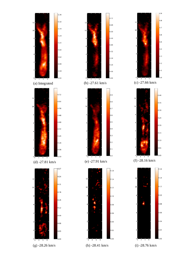
Figure 4: (a) is ¹³CO optical depth integrated map and (b–i) are ¹³CO optical depth channel maps.

4 Isotopic ratios

To find the ¹²CO/¹³CO ratio of the globule, we first regrid the ¹³CO integrated intensity map so that the corresponding pixel coordinates match to those of the ¹²CO map, with both maps in units of flux. To minimise the effects of resolution on the division in the border region, we assign the same restoring beam size for both maps. We create a binary mask that picks only the regions where the ¹³CO emission is above the $3\sigma_{13}$ level. The created mask is then applied to both the ¹²CO and ¹³CO integrated intensity maps in order to avoid thermal noise in the ratio calculation. We find that the ¹²CO/¹³CO line ratio is not uniform throughout the cometary knot. The edges and the core of the globule present different values of ¹²CO/¹³CO, as illustrated in Fig. 5. In the inner parts of the head and the tail, the observed isotopic line ratio is $<$4, with particularly low values ($\sim$2) in the central part. The ratio tends to be higher in the edges of the tail region, reaching up to $\sim$11. Given the age and the physical conditions inside the Helix nebula, the underlying isotopic ratio ¹²C/¹³C is expected to be uniform.

An isotope-selective-photo-dissociation mechanism could be a reason for the variable ¹²CO/¹³CO line ratio (Saberi et al., 2019). According to Szűcs et al. (2014), the photo-dissociation process in a molecular cloud is closely related to the CO density of the region in the cloud. At relatively low-density, ¹²CO is self-shielded from the UV radiation from the CS because the rates at which the photo-dissociation and the ¹²CO production processes occur are similar. On the other hand, at those density levels, ¹³CO is not as effectively shielded due to its lower abundance and its absorption properties. In higher density regions, both ¹²CO and ¹³CO are effectively shielded yielding to a decrease in the ratio. The selective photo-dissociation is dominant mainly in low density regions such as in the extended tail of the globule, and could be the reason behind the observed high values of the ¹²CO/¹³CO line ratio ($\sim$11). However, it does not explain the low values of the ratios. These are more likely due to optical depth effects.

In section 3.3, we find that ¹³CO is mostly optically thin, whereas ¹²CO is highly optically thick. The non-uniformity of the optical depth of the ¹³CO lines along the globule as seen in Fig. 4 is likely to be the main reason for the non-constant observed isotopic ratio. The lowest ¹²CO/¹³CO line ratio observed in the centre of the globule corresponds to the highest optical depth values, i.e. optically thick ¹²CO region. However, the extended tail of the globule is likely to be optically thin in ¹²CO. The emission from this optically thin region would therefore give a better estimate of the true ¹²CO/¹³CO ratio. Using Fig. 5, we find that the ¹²CO/¹³CO intensity ratio corresponding to this region optically thin in ¹²CO is around $11\pm 1$. We take this value of $\sim$11 as the ¹²CO/¹³CO intensity ratio of the whole globule corrected for optical depth. For optically thin lines, a first estimate of the ¹²C/¹³C isotopic ratio can be calculated using the correlation between the ¹²C/¹³C and the ¹²CO/¹³CO intensity ratio given by

$${}^{12}\textmd{C}/^{13}\textmd{C}=\frac{I(^{12}\textmd{CO($J\,\to\,J$--1)})}{I(^{13}\textmd{CO($J\,\to\,J$--1)})}\times\bigg{(}\frac{\nu_{{}^{12}\textmd{CO($J\,\to\,J$--1)}}}{\nu_{{}^{13}\textmd{CO($J\,\to\,J$--1)}}}\bigg{)}^{-3}\textmd{ , }$$ (4)

where $I(^{12}\textmd{CO})$ and $I(^{13}\textmd{CO})$ are the intensities of the ¹²CO and ¹³CO lines, respectively. We use the derived optical depth corrected ¹²CO/¹³CO intensity ratio of $\sim$11 as the line intensity ratio and obtain ¹²C/¹³C $\sim$10.

(a)

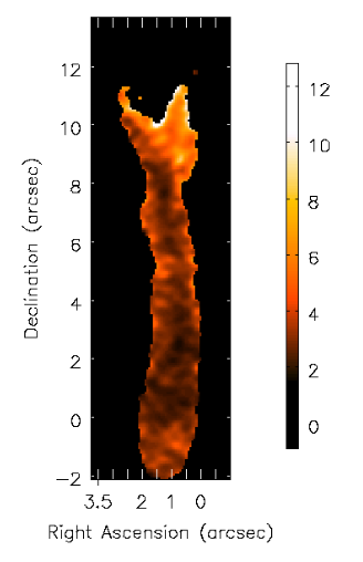
(b)

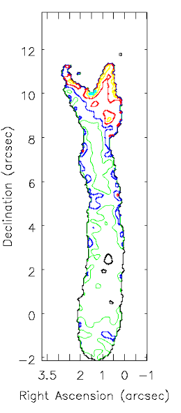
Figure 5: ¹²CO/¹³CO ratio map integrated over the velocity axis, in units of flux. The ratio increases towards the tail of the globule. The central region of the knot presents very low ratio ($<4$). The extended part of the tail has a ratio of $\sim$6, reaching up to $>$10 in the edges. The contours in (b) have ratio values of 2 (black), 3 (green), 4 (blue), 6 (red), 8 (yellow) and 11 (cyan).

We follow the same procedure to determine the C¹⁶O/C¹⁸O ratio. The observed ratio varies from $5$, in the inner parts of the globule, to $>20$ in the outer regions. This C¹⁶O/C¹⁸O intensity ratio can be suppressed by optical depth effects. As ¹³CO and C¹⁸O are both mostly optically thin, we use the ¹³CO/C¹⁸O ratio to derive the optical depth-corrected C¹⁶O/C¹⁸O ratio. We find a mean ¹³CO/C¹⁸O value of $\sim$12. As the ¹²CO/¹³CO line ratio is $\sim 11$, the C¹⁶O/C¹⁸O line ratio is therefore estimated to be $\sim$132. To obtain the ¹⁶O/¹⁸O isotopic ratio, we use (e.g. De Nutte et al., 2017)

$${}^{16}\textmd{O}/^{18}\textmd{O}=\frac{I(\textmd{C}^{16}\textmd{O($J\,\to\,J$--1)})}{I(\textmd{C}^{18}\textmd{O($J\,\to\,J$--1)})}\times\bigg{(}\frac{\nu_{\textmd{C}^{16}\textmd{O($J\,\to\,J$--1)}}}{\nu_{\textmd{C}^{18}\textmd{O($J\,\to\,J$--1)}}}\bigg{)}^{-3}\textmd{ , }$$ (5)

where $I($C${}^{16}\textmd{O})$ and $I($C${}^{18}\textmd{O})$ are the intensities of the C¹⁶O and C¹⁸O lines, respectively. We find ¹⁶O/¹⁸O$\simeq$115.
The ¹³CO/C¹⁸O line ratio may be underestimated: with a maximum optical depth of $\tau_{13}=0.99$, a part of the real ¹³CO emission can be undetected. However, we assumed a constant excitation temperature which may have an effect on the optical depth calculation. The emission detected is from the coldest optically thick ¹²CO line. The optically thin ¹³CO and C¹⁸O emission could trace warmer gas, with a higher limit of 185 K for the C¹⁸O line. Increasing the value of $T_{\textmd{ex}}$ in Eq. 1 would give lower values of the ¹³CO and C¹⁸O optical depths. With an excitation temperature of 60 K, we obtain a maximum ¹³CO optical depth of 0.34. Furthermore, it is important to point out that the ratios obtained are from potentially ¹²CO optically thin regions, based on the assumption that the optical depth of ¹²CO is higher than the optical depth of ¹³CO by a factor of 10 (section 3.3).


The derived isotopic ratios depend on the optical depth of the ¹²CO line which is not well constrained. The AGB models of Karakas & Lugaro (2016) are used to compare these ratios with what is predicted by those models. This is depicted in Fig. 6 which shows the surface abundance ratios at the end of the AGB evolution. The values prior to the last thermal pulse only differ slightly from these values. Models are shown for solar metallicity (Z=0.014: triangles and drawn lines) and for supersolar metallicity (Z=0.03: square and dashed lines). Karakas & Lugaro (2016) present models with different mixing assumptions. This is the reason that at the same stellar mass, several values may be shown. The drawn and dashed line present an ensemble average, but the points show the spread at each mass.
An important constraint is the ¹⁶O/¹⁸O ratio. In the models, for initial stellar masses above 4-5 M_⊙, this ratio becomes very large ($>10^{6}$) because ¹⁸O is burned. The C¹⁸O detection shows that the progenitor mass must be below this range.
The second constraint comes from the suggestion that the dust in the helix is carbonaceous (Van de Steene et al., 2015). The chemical nature of the Helix nebula has been a subject of debate in the literature. Henry et al. (1999) found that oxygen is more abundant than carbon in the Helix nebula using atomic emission lines. The detection of carbon-rich molecules in the nebula, however, led to the conclusion of its carbon molecular nature (Cox et al. 1998, Tenenbaum et al. 2009). In recent studies (e.g. Van de Steene et al. 2015), the Helix nebula is treated as a carbon-rich nebula based on the emissivity index of the dust emission. Carbonaceous dust requires that C/O $>1$. As shown in Fig. 6, for the Karakas & Lugaro (2016) models this happens for initial stellar masses between 1.5 and 4.5 M_⊙ at solar metallicity.
Within this mass range, the isotopic ratios found here are not reproduced by the models. The ¹²C/¹³C ratio is above 50 in all models, due to the fact that the ¹²C dredge-up is needed to form a carbon star. Outside the carbon star range, the ¹²C/¹³C$\sim 10$ is found for high masses but this mass range is excluded by the ¹⁸O detection. Elsewhere, the ¹⁶O/¹⁸O ratio is always around 700, rather than 115 as found here.
An important diagnostic is the ratio between ¹⁶O/¹⁸O and ¹²C/¹³C, which is around 10 in our data. Both parts of this ratio depend in the same way on the ¹²CO line, and as long as both the ¹³CO and C¹⁸O line are optically thin, this ratio should come out correct. If the ¹³CO line is optically thick, the ratio becomes a lower limit. Figure 6 shows the models for this ratio against ¹²C/¹³C. For the observed value, ¹²C/¹³C$\sim 50$, while for higher values it reduces. Comparing this to the models gives a possible mass around 2 M_⊙. There is a second solution around 4 M_⊙. Because of the steep initial mass function, there is some preference for the lower mass.
For this result to be correct, the ¹²C/¹³C ratio derived here would need to be underestimated, and therefore the ¹²CO line would need to have a higher optical depth. We cannot confirm this with the available data.

Figure 6: Predicted isotopic and elemental abundance ratios at the end of the AGB, as function of initial stellar mass, taken from Karakas & Lugaro (2016).

We can also compare these predictions with observations of the ¹²C/¹³C isotopic ratios of presolar grains in Zinner (2014). The optical depth-corrected ¹²C/¹³C isotopic ratio of the C1 globule is lower than the ¹²C/¹³C ratios of mainstream (20<¹²C/¹³C$<$100) and type Z silicon carbide grains (¹²C/¹³C$<$100), which originate from AGB carbon stars (Zinner, 2014). The presolar grains show isotopic ratios that agree with stellar models.
We can also compare with observations of AGB stars. The derived ¹²C/¹³C ratio is within the range of the ¹²C/¹³C ratios for different SC-type AGB carbon stars (C/O$\sim 1$) in Abia et al. (2017), which range from 5 to 35. However, the obtained ¹⁶O/¹⁸O ratio of 115 in the Helix is much lower than the ¹⁶O/¹⁸O ratios in Abia et al. (2017) for different SC-type AGB carbon stars, ranging from $400$ to $1250$.
This discussion shows that the ¹³C¹⁶O/¹²C¹⁸O is an important observational constraint in the comparison with the models. In the case of the Helix, the comparison raises the possibility that the optical depth of the ¹²CO line has been underestimated.

5 Mass

5.1 Molecular mass

We use the CO lines as H₂ tracers to estimate the molecular mass of the C1 globule.
The column densities of ¹³CO and C¹⁸O, N(¹³CO) and N(C¹⁸O), are calculated using the column density in the upper state $N_{\textmd{$J=2$}}$ (e.g. Nishimura et al., 2015)

$$N_{\textmd{$J=2$}}^{\textmd{${}^{13}$CO}}=1.65\times 10^{16}\Bigg{[}\textmd{exp}\Bigg{(}\frac{10.58}{T_{\textmd{ex}}}\Bigg{)}-1\Bigg{]}^{-1}\int\tau_{13}(v)\,dv\,\textmd{cm${}^{-2}$}$$ (6)

$$N_{\textmd{$J=2$}}^{\textmd{C${}^{18}$O}}=1.64\times 10^{16}\Bigg{[}\textmd{exp}\Bigg{(}\frac{10.54}{T_{\textmd{ex}}}\Bigg{)}-1\Bigg{]}^{-1}\int\tau_{18}(v)\,dv\,\textmd{cm${}^{-2}$}$$

where $T_{\textmd{ex}}=30\,\textmd{K}$ is the excitation temperature, $v$ is the velocity centre and $dv=0.05$ $\textmd{km}\,\textmd{s}^{-1}$ is the velocity width. $\tau_{13}$ and $\tau_{18}$ are the optical depths of ¹³CO and C¹⁸O calculated in section 3.3. The total column density is obtained using (Nishimura et al., 2015)

$$N(\textmd{${}^{13}$CO})=N_{\textmd{$J=2$}}^{\textmd{${}^{13}$CO}}\,\frac{Z}{2\,J+1}\,\textmd{exp}\bigg{[}\frac{h\,B_{0}\,J(J+1)}{k\,T_{\textmd{ex}}}\bigg{]}\,\textmd{cm${}^{-2}$}\,\textmd{,}$$ (7)

$$N(\textmd{C${}^{18}$O})=N_{\textmd{$J=2$}}^{\textmd{C${}^{18}$O}}\,\frac{Z}{2\,J+1}\,\textmd{exp}\bigg{[}\frac{h\,B_{0}\,J(J+1)}{k\,T_{\textmd{ex}}}\bigg{]}\,\textmd{cm${}^{-2}$}\,\textmd{.}$$

$N_{\textmd{$J=2$}}^{\textmd{${}^{13}$CO}}$ and $N_{\textmd{$J=2$}}^{\textmd{C${}^{18}$O}}$ are the column density in the state $J=2$ for ¹³CO and C¹⁸O derived in equation (6), respectively. $B_{0}$ is the rotational constant, where $B_{0}=5.51\times 10^{10}\,$s^-1 for ¹³CO and $B_{0}=5.49\times 10^{10}\,$s^-1 for C¹⁸O (Nishimura et al., 2015). $h$ and $k$ are the Planck and Boltzmann constant, respectively. $T_{\textmd{ex}}$ is the excitation temperature obtained in equation (1). $Z$ is the partition function given by (Nishimura et al., 2015)

$$Z=\sum_{J=0}^{\infty}(2\,J+1)\,\,\textmd{exp}\bigg{[}-\frac{h\,B_{0}\,J(J+1)}{k\,T_{\textmd{ex}}}\bigg{]}$$ (8)

which can be approximated as follows for diatomic linear molecules (Mangum & Shirley, 2015)

$$Z\simeq\frac{k\,T}{h\,B_{0}}+\frac{1}{3}+\frac{1}{15}\bigg{(}\frac{h\,B_{0}}{k\,T}\bigg{)}+\frac{4}{315}\bigg{(}\frac{h\,B_{0}}{k\,T}\bigg{)}^{2}+\frac{1}{315}\bigg{(}\frac{h\,B_{0}}{k\,T}\bigg{)}^{3}+...\,\textmd{.}$$ (9)

Equation (9) is accurate to $<$1 percent for $T_{\textmd{ex}}>\,$2 K, even with the first two terms only (Mangum & Shirley, 2015).

The derived column densities $N(\textmd{${}^{13}$CO})$ and $N(\textmd{C${}^{18}$O})$ are converted to ¹²CO column densities by multiplying them with the corresponding isotopic ratios corrected for optical depth derived in section 4. We obtain the two-dimensional ¹²CO column density distributions, N(¹²CO), integrated over all velocity channels.
We use the distance to the Helix nebula of 201$\pm 4\,$pc derived from the parallax of the Helix measured by Gaia Collaboration (2018) (Gaia mission: Gaia Collaboration et al., 2018; Luri et al., 2018), and assume a CO/H₂ ratio of 6$\,\times 10^{-4}$ based on the CO/H abundance ratio of $\sim$3$\,\times 10^{-4}$ in the Helix nebula in Huggins et al. (1992); Huggins et al. (2002). This assumed CO/H₂ ratio is in agreement with the ratio found by De Beck et al. (2010) for S-type stars. We obtain a molecular mass of $1.8\,\times 10^{-4}\,$$\textup{M}_{\odot}$ from ¹³CO and of $1.5\times 10^{-4}\,$$\textup{M}_{\odot}$ from the C¹⁸O emission.

We look into the distribution of the mass in the knot using the head and tail definition given in section 3.1. We find that the tail has a mass of $1.7\,\times 10^{-4}\,$$\textup{M}_{\odot}$ from ¹³CO and $1.5\,\times 10^{-4}\,$$\textup{M}_{\odot}$ from C¹⁸O, whereas the head only accounts for $1.3\,\times 10^{-5}$ and $7.7\,\times 10^{-6}\,$$\textup{M}_{\odot}$ from ¹³CO and C¹⁸O, respectively. This means that the majority of the CO in the knot is carried by the tail. The ¹³CO column density distribution of the head and the tail of the C1 globule is illustrated in Fig. 7 and shows that the tail is denser than the head.

These derived masses are $>$9 times higher than the mass found by Huggins et al. (2002, 1992) for C1 using CO(1–0) observations, and Young et al. (1997) for different knots using CO(2–1), ranging from 5$\,\times 10^{-6}$ to 2$\,\times 10^{-5}\,$$\textup{M}_{\odot}$. The difference between our result and the masses obtained in those previous studies is mainly due to optical depth. Huggins et al. (1992); Huggins et al. (2002) calculated the molecular mass of the C1 globule from CO(1–0) emission assuming that ¹²CO is optically thin. However, with an optically thick ¹²CO and making use of its optically thin isotopes, ¹³CO and C¹⁸O, we derive the molecular mass considering the ¹²CO column density corrected for optical depth. Without optical depth correction, the molecular mass would be $\sim$6$\,\times 10^{-5}\,$$\textup{M}_{\odot}$, which is closer to the mass found by Huggins et al. (2002). In addition, the mass derived from some of these prior studies are obtained from a beam-averaged column density from unresolved knots which led to an underestimation due to beam dilution.
Uncertainties lie in the CO/H₂ conversion factor and the LTE assumption, which have been found to estimate the molecular mass with a discrepancy of up to $\sim 30$ percent (Szűcs et al., 2016).

With $23\,000$ globules in the Helix nebula (Meixner et al., 2005) with individual masses of $\sim$2$\,\times 10^{-4}\,$$\textup{M}_{\odot}$, the total mass of the globules would give a value much higher than the mass of the entire nebula, M${}_{\textmd{Helix}}=\,\sim$1.5 $\textup{M}_{\odot}$ (Speck et al., 2002). This could mean that the Helix nebula is, in fact, a combination of condensed globules. However, an overestimation of the number of the knots is possible, though Matsuura et al. (2009) found a higher number of globules by almost a factor of 2. Furthermore, globules do not necessarily have the same mass. As seen in Fig. 3 in Meaburn et al. (1998) where C1 is designated 1, this particular globule is relatively large, hence more massive than some of its companions. In addition, our results show that the mass of C1 is mainly found in the tail. As only the knots in the inner part like C1 are observed to exhibit distinct tails (e.g. Matsuura et al. 2009), the knots in the outer regions could have a much lower mass than those located closer to the CS.

The derived physical parameters of the C1 globule are presented in Table 1.

Table 1: Derived properties of the C1 globule.

	Size	Flux	Flux density	Mass of the head	Mass of the tail	Total mass
	[arcsec $\times$ arcsec]	[Jy$\,\textmd{km}\,\textmd{s}^{-1}$]	[mJy]	[$\textup{M}_{\odot}$]	[$\textup{M}_{\odot}$]	[$\textup{M}_{\odot}$]
CO	$\sim 2\,\times\,16$	14.4	-	-	-	-
13CO	$\sim 2\,\times\,14$	$3.5$	-	$1.3\times 10^{-5}$	$1.7\times 10^{-4}$	$1.8\times 10^{-4}$
C18O	$\sim 1-2\,\times\,11$	$0.18$	-	$7.7\times 10^{-6}$	$1.5\times 10^{-4}$	$1.5\times 10^{-4}$
Dust	-	-	$0.33$	$2.7\times 10^{-6}$	$2.8\times 10^{-6}$	$5.5\times 10^{-6}$

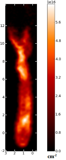
Figure 7: ¹³CO Column density map of the C1 globule. The axes are the same as in Fig. 4. The tail is denser than the head.

5.2 Gas mass from dust observation

Figure 8 shows the $1.2\,\textup{mm}$ continuum map of the C1 globule. Free-free emission is not expected to be important in the knot, so the continuum emission is entirely associated with dust, with a total flux density of $(3.3\pm 0.2)\times 10^{-4}$Jy. There is no zero-spacing problem for the narrow tail in the interferometric data: all flux is in principle detected. We do not consider emission below 2$\sigma$ ($\sigma=20\,\mu$Jy beam^-1). Figure 8 shows that dust in the tail is weaker compared to the observed CO emission. Dust is only detected at a few locations throughout the tail of the knot whereas the head region seems to present a relatively concentrated dust emission, accounting for $\sim 50$ percent of the total flux density.

We calculate the gas mass of the globule using the measured dust emission. On the assumption that grains in the nebula are mainly amorphous carbon, Van de Steene et al. (2015) found that the temperature of the dust in the Helix nebula varies from $22$ to $42\,\textmd{K}$ with a mean value of $30.8\pm 1.4\,\textmd{K}$. We use

$$M_{\textmd{gas}}=\frac{10^{-26}}{T_{\textmd{dust}}\,\chi_{\textmd{d}}}\frac{S_{\nu}\,D^{2}\,\lambda^{2}}{2\,\gamma K_{\textmd{d}}\,k_{\textmd{B}}}\frac{1}{2}10^{-33}\,\textup{M}_{\odot}\$$ (10)

to find the mass of the gas (e.g. Evans et al. 2004), assuming that the emission is under the Rayleigh-Jeans approximation. The parameters used are as follows. $T_{\textmd{dust}}$ is the mean temperature of the dust, found by Van de Steene et al. (2015). The temperature of the dust in the Helix nebula is similar to the excitation temperature of the CO lines obtained in section 5.1. This is indicative that molecular gas and dust coexist inside the globule. $K_{\textmd{d}}$ corresponds to the absorption coefficient. We use $K_{\textmd{d}}=20\,\,\textmd{cm}^{2}\,\textmd{g}^{-1}$ taken from Mennella et al. (1998) for amorphous carbon dust grain at $1\,\textmd{mm}$ and at $20\,\textmd{K}$, which is the closest to our data specifications. $\chi_{\textmd{d}}$ is the dust–to–gas mass ratio. Its value varies in the literature, from $\chi_{\textmd{d}}\simeq 1\textmd{:}55$ in O’Dell (1998) and Henry et al. (1999) to $\chi_{\textmd{d}}=1\textmd{:}150$ in Sodroski et al. (1994) and O’Dell et al. (2005). Here we use $\chi_{\textmd{d}}=1\textmd{:}100$ as in Meaburn et al. (1992). $D$ is the distance to the Helix nebula in cm, $S_{v}$ is the flux density in Jy and $\lambda$ represents the wavelength in m. $k_{\textmd{B}}$ is the Boltzmann constant and $\gamma$ is a constant that depends on the optical thickness of the dust shell. $\gamma=1$ for an optically thin dust shell, while $\gamma=2$ if the shell is optically thick. At this wavelength, dust emission is optically thin.

We obtain a dust mass of 5.5$\,\times 10^{-8}\,$$\textup{M}_{\odot}$ and a gas mass of 5.5$\,\times 10^{-6}\,$$\textup{M}_{\odot}$. This gas mass is $\sim$2 times lower than the globule mass in Meaburn et al. (1992) and in Meaburn et al. (1998) ($\sim 10^{-5}$ $\textup{M}_{\odot}$) from dust observation which took into account the emission in the head of the globule only. The masses of the knot derived from the CO lines (section 5.1) and dust emission differ by a factor of > 25. Figure 8 suggests that dust in the tail is much weaker than the observed CO, which is reflected in the mass derived from dust emission. The obtained gas mass is on the order of the molecular mass of the head of the globule that we derived from C¹⁸O. As the detected dust emission is weak, the 2$\sigma$ cut-off could result in an underestimation of the total gas mass.

The value of the dust–to–gas mass ratio $\chi_{\textmd{d}}$ in the Helix nebula is uncertain. With a dust–to–gas mass ratio of $1\textmd{:}150$ in the Helix (Sodroski et al. 1994, O’Dell et al. 2005), we find a gas mass of 8.3$\,\times 10^{-6}$ $\textup{M}_{\odot}$. With the commonly used value of dust–to–gas mass ratio for the Helix nebula $\chi_{\textmd{d}}\simeq 1\textmd{:}55$ (O’Dell 1998, Henry et al. 1999), the corresponding gas mass is 3$\,\times 10^{-6}$ $\textup{M}_{\odot}$.
Non-negligible uncertainties lie in the absorption coefficient. According to Mennella et al. (1998), the absorption coefficient decreases as the wavelength increases. The value of $K_{\textmd{d}}$ that we used to calculate the dust mass is for a 1 mm-wave at 20 K, so, a more accurate value of $K_{\textmd{d}}$ corresponding to the observed 1.2 mm dust emission at $30\,$K would give a higher gas mass.

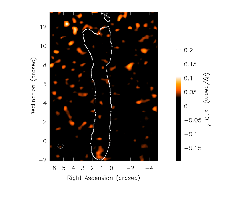
Figure 8: Dust continuum map with ¹²CO contour at a level of $20\,\textmd{mJy}\,\textmd{beam}^{-1}$. The restoring beam (in $\textmd{arcsec}\times\textmd{arcsec}$) is at the bottom left of the map with a size of $0.40\times 0.34$.

5.3 Clumping

In section 4, we mentioned the possibility of a non-constant excitation temperature. With the resolution of our ALMA data, we assumed a smooth CO distribution, but the existence of unresolved clumps with different temperatures and different optical depths throughout the globule could be possible. The presence of higher density molecular clumps that are smaller than the beam size in the knot would have led to an overestimation of the molecular mass, as the brightness measured is averaged over the beam. Knowing the size and the density of those clumps would give a better estimate of the molecular mass of the knot. With a beam dilution effect of $\sim$10 due to high density clumps, the molecular mass after beam dilution correction would be similar to the gas mass of C1 and other knots from dust emission derived by Meaburn et al. (1992, 1998) and to its molecular mass in previous studies (e.g. Young et al., 1997; Meaburn et al., 1998; Huggins et al., 2002). Clumps in the C1 globule would also affect the calculation of the optical depth and the isotopic ratios in the globule, and therefore, influence the determination of the chemical nature of the Helix nebula. However, Meaburn et al. (1998) reported a uniform H₂ density throughout the head of the C1 globule. Higher angular resolution data, in the optically thin C¹⁸O line in particular, are needed in order to investigate the likelihood of clumping in the C1 knot.

6 Origin and evolution

The processes responsible for the origin and evolution of the cometary knots in the Helix nebula are uncertain. Are they created in the AGB wind, in which case they would be described as primordial, or in the planetary nebula, i.e. after the AGB phase? A primordial nature of the globules was suggested by Dyson et al. (1989) where relatively massive density enhancements are created in the atmosphere of the AGB star and somehow survive to the PN transition. To test this theory, Huggins & Mauron (2002) looked for the presence of globule-like structures in the molecular halo of the young planetary nebula NGC 7027 and in the atmosphere of the AGB star IRC+ 10216 without success. On the other hand, non-primordial globules would imply that the physical conditions inside the nebula fostered the creation of cool molecular clumps. Matsuura et al. (2009) analysed the likelihood of the two scenarios and reported that part of the H₂ in the knots could be primordial, but the formation and survival of H₂ in dense and ionized regions inside PNe are also possible, as investigated by Aleman & Gruenwald (2004). The effect of spiral wave compression from the interaction with a binary companion could also result in the formation of clumps in the AGB wind.

Tail formation

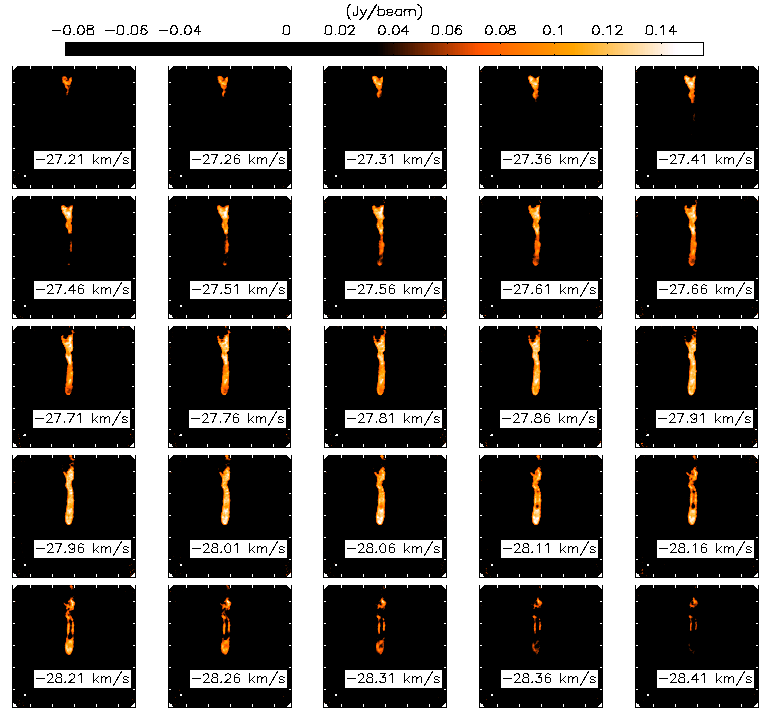
Figure 9: ¹²CO(2–1) channel maps of the CO globule centred at the velocities in the bottom left of each channel. The channels are $0.05\,\textmd{km}\,\textmd{s}^{-1}$ wide. y and x axes are the same as in Fig. 1.

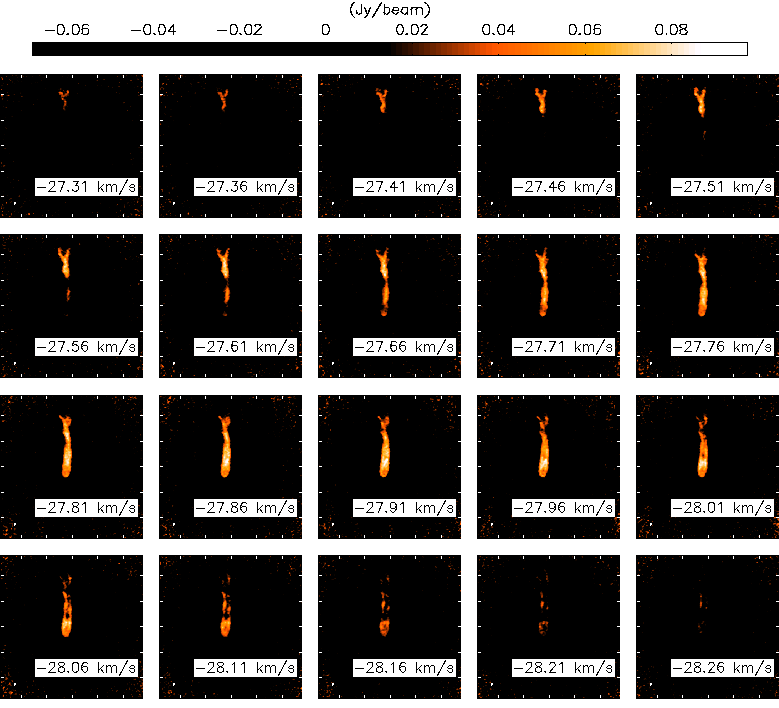
Figure 10: Same as Fig. 9 for ¹³CO(2–1).

Different models have been proposed to describe the formation of globule tails, the most common ones being the stream, the photoevaporation and the shadowing models. Those models are not intended to explain the origin of the density enhancement, i.e. whether they are primordial or not, but assume the presence of a dense core and describe the mechanisms that shape those density enhancements into comet-like objects. In the following, we will discuss those three models and see how consistent they are with our data.

The stream model consists of an ambient wind and the flow from the knot interacting with each other. The velocity difference between the globule and the ambient wind results in a shock that creates the optical bow-shape of the head. The material from the head is swept by the wind to form the tail (Dyson et al., 2006). The nature of the wind differs for different models. Meaburn et al. (1996) suggested that expanding diffuse shells or the fast wind from the CS could interact with the dense cores and create the tails. Meaburn et al. (1992) estimated the lifetime of globules and compared it to the lifetimes of the fast and expansion winds and found that both types of winds can potentially interact with the dense cores to produce the tails of cometary knots. Furthermore, an evolution in the nature of the ambient wind, from subsonic to supersonic, would lead to meandering in the tails of the globule. More recently, Meaburn & Boumis (2010) described the stream model as particle winds from the CS sweeping past the slowly expanding system of knots. According to the stream model, the system of cometary knots has a typical radial expansion velocity of around $10\,\textmd{--}\,14\,\textmd{km}\,\textmd{s}^{-1}$ (Meaburn et al., 1996; Meaburn et al., 1998). From theoretical simulations of individual knots in [N ii], Meaburn et al. (1998) suggested that the wind-swept model would produce an ablation flow velocity of $\sim 10\,\textmd{km}\,\textmd{s}^{-1}$.
We look for a velocity gradient between the head and the tail of the C1 globule to test the ablation of the head by an ambient wind. Figure 9 and Fig. 10 show the ¹²CO and ¹³CO(2–1) channel maps of C1 with a velocity width of $0.05\,\textmd{km}\,\textmd{s}^{-1}$. In the ¹³CO channel maps, the tail is a few arcseconds shorter and observable in fewer channels than in ¹²CO. We notice that only the tail is visible in the maps at the top channels (at $\sim-27.2\,\textmd{km}\,\textmd{s}^{-1}$) which would suggest that there is head ablation. However, the head and the tail are both detected at velocities $\sim-28.3$ $\textmd{km}\,\textmd{s}^{-1}$. The centre of the tail has a velocity about $0.5\,\textmd{km}\,\textmd{s}^{-1}$ redshifted from the cocoon around it. Figure 11 illustrates the velocity distribution along the declination axis and shows a differential movement between the head and the tail of the globule, of around $0.4$ and $0.5\,\textmd{km}\,\textmd{s}^{-1}$ along the line of sight for ¹²CO and ¹³CO, respectively. This velocity gradient is not enough to support a wind-swept pattern. Figure 12 shows the velocity along the right ascension axis for different declination for the ¹²CO emission. The velocity range is roughly constant in the head and the mid-region of the tail, but it presents a drop of $\sim 0.4\,\textmd{km}\,\textmd{s}^{-1}$ towards the extended tail, around $+\,10.5^{\prime\prime}$ from the tip of the head. Those values are far from the $10\,\textmd{km}\,\textmd{s}^{-1}$ ablation flow velocity expected and, thus, do not confirm the stream model. Our result is in agreement with Huggins et al. (2002) who found an observable velocity gradient of $0.2\,\textmd{km}\,\textmd{s}^{-1}$ in the line of sight and of $0.8\,\textmd{km}\,\textmd{s}^{-1}$ in a radial direction. With a velocity flow of $\sim 1\,\textmd{km}\,\textmd{s}^{-1}$, the end of the tail of the globule would be reached in around 10${}^{4}\,$yr.

(a)

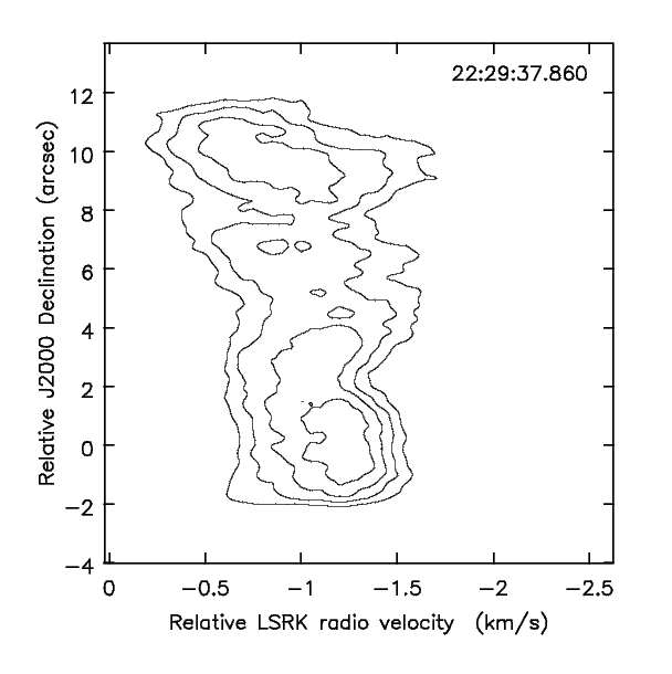
(b)

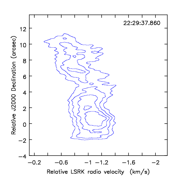
Figure 11: Right ascension averaged velocity strip maps of the C1 globule along the declination axis and centred at right ascension given in the top right of each map. (a): ¹²CO(2–1) and contour intervals are $0.0108\,\textmd{Jy}\,\textmd{beam}^{-1}$. (b): ¹³CO (2–1) and contour intervals are $0.006\,\textmd{Jy}\,\textmd{beam}^{-1}$.

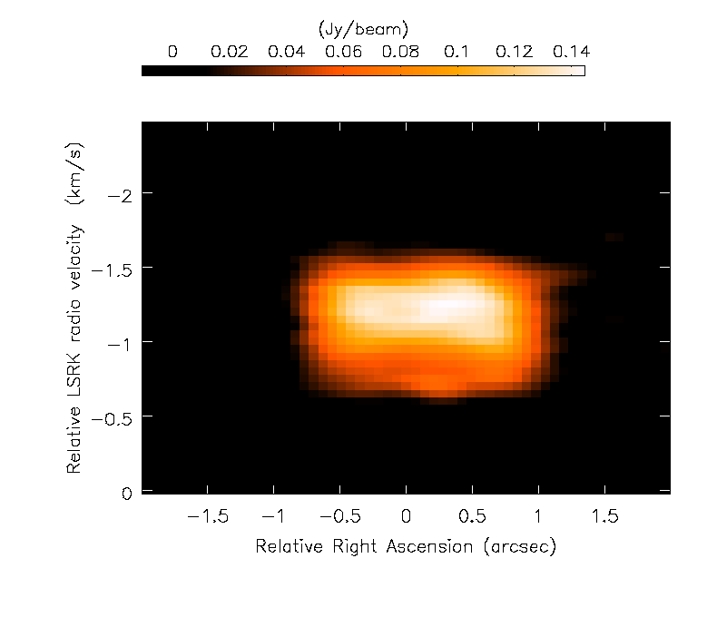
(a)	(b)
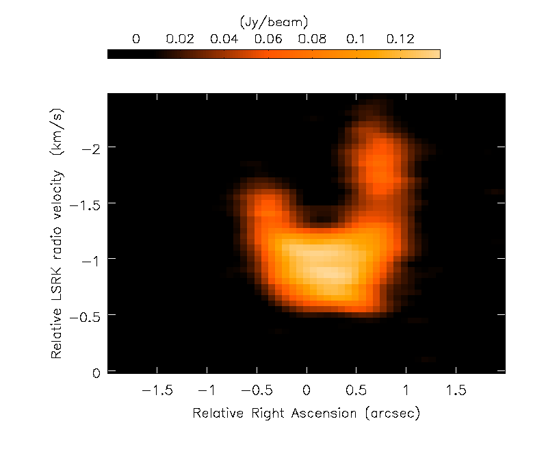
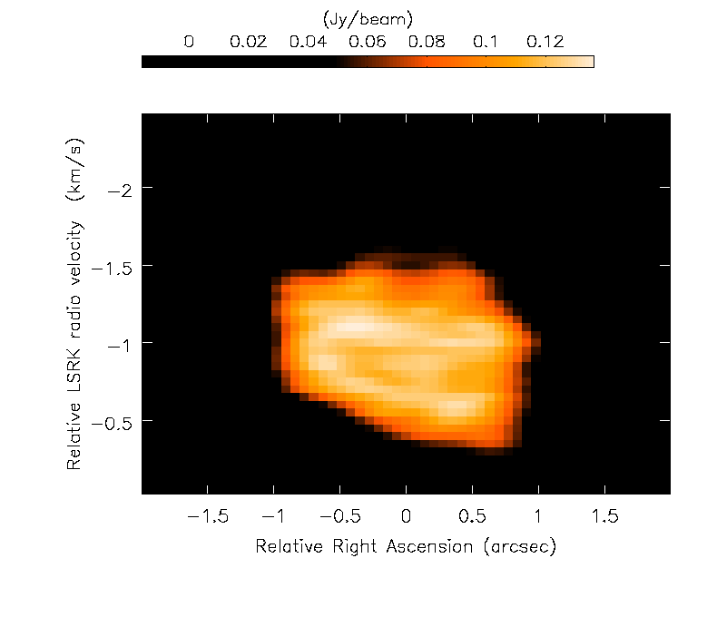
(c)	(d)

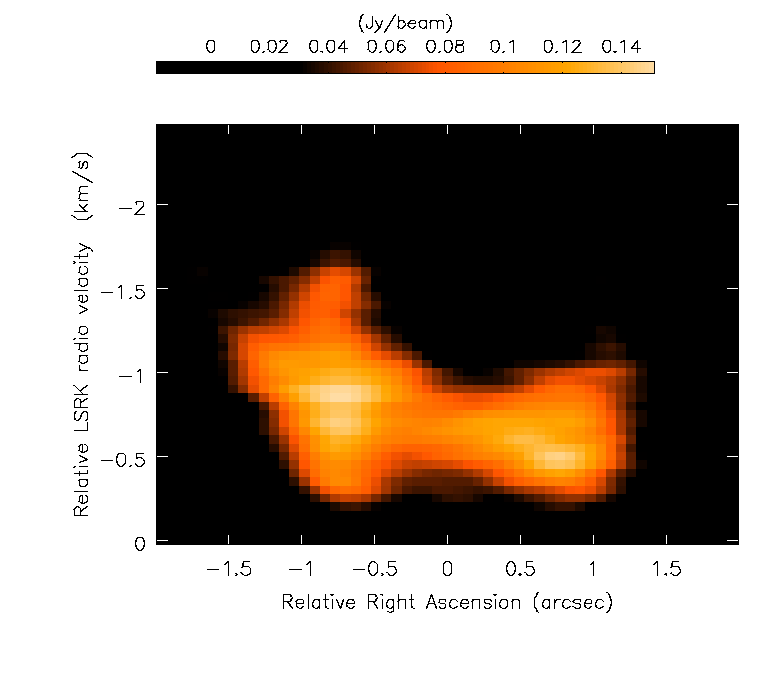
Figure 12: Velocity against right ascension at different declinations for ¹²CO. (a): head of the globule at a declination of $-0.5^{\prime\prime}$ (see Fig. 1 for position reference), (b): mid-tail at $+\,5.5^{\prime\prime}$, (c): tail at $+\,9^{\prime\prime}$ and (d): extended tail at $+\,10.5^{\prime\prime}$.

In addition, as mentioned in section 3.1 and 5.1, our results highlight the molecular nature of the tail of the C1 globule. Do the molecules in the tail originate from the head? Is the interaction strong enough to sweep the needed quantity of material from the head to create the heavily molecular tail? This model seems unlikely to explain our observations, in particular, the multipeak structure of the globule and the high mass of the tail. None the less, the meandering of the tail could be the consequence of streaming motion instabilities (e.g Dyson et al. 2006). We conclude that the stream model alone does not describe the formation of the tail of the C1 globule.

From Fig. 5, we observe that the highest ¹²CO/¹³CO line ratio is in the extended tail (at $\sim+\,10^{\prime\prime}$). In section 6, we find that the velocity in this region is not the same as the velocity observed in the rest of the globule, which may indicate that the corresponding radiative environments are different. Therefore, we do not exclude the possibility of the observed extended tail to represent a different globule.

Cantó et al. (1998) proposed the shadowing by density enhancement model to explain the origin of the cometary tails of the knots in the Helix nebula. In this model, the initial dense core can be large and is located in the photoionized region of the nebular envelope. The UV radiation from the CS hits the head but does not directly reach the tail region which is shadowed. The tail of the core is then illuminated by the diffuse radiation. In this model, the shadow region has a neutral inner core with a bright rimmed trailing envelope.
Two versions of the globule shaping process by shadowing are possible (Huggins et al., 1992). The first one consists of the shadowing of preexisting molecules close to the central star overrun by the ionization front of the nebula leading to the creation of molecular tails. The second version assumes that the tail and the head are created simultaneously. The latter would be more consistent with our data given the high molecular mass of the tail.
The shadowing model can explain the molecular nature of the tail that we observe in CO, and could also explain the presence of the different peaks in the globule. Moreover, the flux of the radiation from the CS of the Helix nebula (Kaler et al., 1990) is low enough to permit the neutral core to be shielded (Huggins et al., 1992).

In the photoevaporation model (López-Martín et al., 2001), the UV photons from the central star interact with the material of the density enhancement. The surface of the core is heated by the UV radiation and the shock from that interaction creates the crescent tip of the head of the knot observed in optical images (see Fig. 2). The globule slowly evaporates as the nebula expands (Huggins et al., 1992). However, this model does not clearly explain the formation of the tail. It is often combined with other processes such as the stream model, where a wind sweeps the photoionized gas and the neutral material to the tail (Huggins et al. 1992, Matsuura et al. 2009). The photoevaporation model alone does not explain the molecular properties of the knot.

The peaks observed in the body of the globule can also be due to the interaction of globules with one another (Pittard et al., 2005). In the case of the C1 globule, it seems to be fairly isolated. However, the peak observed at $\sim$+$\,8^{\prime\prime}$ (see Fig. 1) can be the relic of the condensation of an other globule.

Matsuura et al. (2009) investigated a certain number of knots in molecular H₂(1-0) and concluded that the stream and photoevaporation models have important contributions to the tail shaping process at the expense of shadowing, whose level of contribution had yet to be proven. However, the shadowing model is the one that best explains our data, as it is the only model that is consistent with a highly molecular tail. A tail formation scenario where the effects of all models are taken into account is desirable, so, we suggest the following combination of models. The initial density enhancement is a large dense core made of gas and dust whose head is hit by UV radiation from the CS, leading to the photoevaporation and shaping of the ionized bow-like head, while the remaining part of the knot is shielded. The diffuse radiation from the head illuminates the shadowed tail and the globule slowly evaporates. This is consistent with Fig. 2, showing an HST optical observation of the ionized head overlaid with our CO data of the C1 globule. Though we did not find any evidence of ablation of the head to support the stream model, we do not exclude the possibility of it being responsible for the meandering of the tail.

Near and distant knots

Globules near and far from the CS present different physical appearances. Globules closer to the CS, like the C1 globule, exhibit a head and a defined extended tail, whether in molecular (H₂) or in [O iii] (in absorption), whereas those in the far side do not present such defined tails and are more numerous (Matsuura et al., 2009). In addition, the bow shape of the ionized head is not always observed for knots located far from the CS. The question of which of those categories represent the younger globules, i.e. their evolution, is directly related to the physical processes responsible for their creation and shaping. Our analysis shows that shadowing and photoevaporation are the main contributors to the shaping of the C1 globule. This may explain why the knots in the outer part do not present visible tails in optical images ( e.g. O’Dell et al. 2004), and lie in dense regions where tails are blended in and indistinguishable in H₂, as imaged by Matsuura et al. (2009). In fact, the high number density of knots in the outer region is expected to make the shielding effect more efficient and, combined with interactions due to the proximity of the globules with one another, reduce the possibility of observing distinct tails. However, their morphological differences have also been suggested to indicate that different processes may be responsible for the shaping of the globules in the inner and outer parts of the nebula (Matsuura et al., 2009).

7 Conclusion

We derived the physical parameters of the C1 globule from new CO observations. With an optically thick ¹²CO line, we found that the molecular mass of the knot may have been highly underestimated by previous studies. The globule has a molecular mass of M${}_{\textmd{knot}}$=$1.8\,\times 10^{-4}\,$$\textup{M}_{\odot}$, which is mainly carried by the tail. With such a mass, we suspect the nebula to be, in fact, condensation of globules, where the knots close to the CS such as C1 are more massive than the ones in the outer region. From dust observation, we find a gas mass of $5.5\times 10^{-6}\,$$\textup{M}_{\odot}$. The optical depth-corrected ¹²C/¹³C and ¹⁶O/¹⁸O ratios are $\sim$10 and $\sim$115, respectively. Those values are not consistent with the carbon and oxygen isotopic ratios of AGB carbon stars. The ¹²CO optical depth may be underestimated. The high derived molecular mass and the low CO isotopic ratios could be the effects of clumping in the globule. Investigating the likelihood of the presence of clumps in C1 would require higher resolution data. The tail formation process is also discussed and our findings are in agreement with the shadowing model combined with photoevaporation. Though our observations did not show strong evidence to support the stream model, we do not exclude its possible contribution to tails meandering. Our data therefore suggest that the shaping of the knots into comet-like structures is likely to happen after photoionization of the nebula, i.e. not during the AGB phase. Our model seems to be compatible with ionized gas observations of the C1 globule, and could also explain why cometary knots near and distant from the CS appear to have different morphologies. Finally, given the multi-peak structure of the globule, the feature observed in the optical depth maps, the high mass of the tail and its slightly shifted velocity, it is possible that the C1 globule actually consists of two different knots.

References

- Abia et al. (2017) Abia C., Hedrosa R. P., Domínguez I., Straniero O., 2017, A&A, 599, A39
- Aleman & Gruenwald (2004) Aleman I., Gruenwald R., 2004, The Astrophysical Journal, 607, 865
- Bachiller et al. (1997) Bachiller R., Forveille T., Huggins P., Cox P., 1997, Astronomy and Astrophysics, 324, 1123
- Cantó et al. (1998) Cantó J., Raga A., Steffen W., Shapiro P. R., 1998, The Astrophysical Journal, 502, 695
- Cox et al. (1998) Cox P., et al., 1998, The Astrophysical Journal Letters, 495, L23
- De Beck et al. (2010) De Beck E., Decin L., de Koter A., Justtanont K., Verhoelst T., Kemper F., Menten K. M., 2010, A&A, 523, A18
- De Nutte et al. (2017) De Nutte R., et al., 2017, Astronomy and Astrophysics, 600, A71
- Dyson et al. (1989) Dyson J., Hartquist T., Pettini M., Smith L., 1989, Monthly Notices of the Royal Astronomical Society, 241, 625
- Dyson et al. (2006) Dyson J., Pittard J., Meaburn J., Falle S., 2006, Astronomy & Astrophysics, 457, 561
- Evans et al. (2004) Evans A., Geballe T., Tyne V., Pollacco D., Eyres S., Smalley B., 2004, Monthly Notices of the Royal Astronomical Society, 353, L41
- Gaia Collaboration (2018) Gaia Collaboration 2018, VizieR Online Data Catalog, p. I/345
- Gaia Collaboration et al. (2018) Gaia Collaboration et al., 2018, A&A, 616, A1
- Henry et al. (1999) Henry R., Kwitter K., Dufour R., 1999, The Astrophysical Journal, 517, 782
- Huggins & Mauron (2002) Huggins P., Mauron N., 2002, Astronomy & Astrophysics, 393, 273
- Huggins et al. (1992) Huggins P., Bachiller R., Cox P., Forveille T., 1992, The Astrophysical Journal, 401, L43
- Huggins et al. (1996) Huggins P., Bachiller R., Cox P., Forveille T., 1996, Astronomy and Astrophysics, 315, 284
- Huggins et al. (2002) Huggins P., Forveille T., Bachiller R., Cox P., Ageorges N., Walsh J., 2002, The Astrophysical Journal Letters, 573, L55
- Kaler et al. (1990) Kaler J. B., Shaw R. A., Kwitter K. B., 1990, The Astrophysical Journal, 359, 392
- Karakas & Lugaro (2016) Karakas A. I., Lugaro M., 2016, ApJ, 825, 26
- López-Martín et al. (2001) López-Martín L., Raga A., Mellema G., Henney W., Cantó J., 2001, The Astrophysical Journal, 548, 288
- Luri et al. (2018) Luri X., et al., 2018, A&A, 616, A9
- Mangum & Shirley (2015) Mangum J. G., Shirley Y. L., 2015, PASP, 127, 266
- Matsuura et al. (2007) Matsuura M., et al., 2007, Monthly Notices of the Royal Astronomical Society, 382, 1447
- Matsuura et al. (2009) Matsuura M., et al., 2009, The Astrophysical Journal, 700, 1067
- McMullin et al. (2007) McMullin J., Waters B., Schiebel D., Young W., Golap K., 2007, in Astronomical data analysis software and systems XVI. p. 127
- Meaburn & Boumis (2010) Meaburn J., Boumis P., 2010, Monthly Notices of the Royal Astronomical Society, 402, 381
- Meaburn et al. (1992) Meaburn J., Walsh J., Clegg R., Walton N., Taylor D., Berry D., 1992, Monthly Notices of the Royal Astronomical Society, 255, 177
- Meaburn et al. (1996) Meaburn J., Clayton C., Bryce M., Walsh J., 1996, Monthly Notices of the Royal Astronomical Society, 281, L57
- Meaburn et al. (1998) Meaburn J., Clayton C., Bryce M., Walsh J., Holloway A., Steffen W., 1998, Monthly Notices of the Royal Astronomical Society, 294, 201
- Meixner et al. (2005) Meixner M., McCullough P., Hartman J., Son M., Speck A., 2005, The Astronomical Journal, 130, 1784
- Mennella et al. (1998) Mennella V., Brucato J., Colangeli L., Palumbo P., Rotundi A., Bussoletti E., 1998, The Astrophysical Journal, 496, 1058
- Nishimura et al. (2015) Nishimura A., et al., 2015, The Astrophysical Journal Supplement Series, 216, 18
- Nishiyama (2018) Nishiyama J. J., 2018, An Introduction to Planetary Nebulae
- O’Dell (1998) O’Dell C., 1998, The Astronomical Journal, 116, 1346
- O’Dell & Handron (1996) O’Dell C., Handron K. D., 1996, The Astronomical Journal, 111, 1630
- O’Dell et al. (2002) O’Dell C., Balick B., Hajian A., Henney W., Burkert A., 2002, The Astronomical Journal, 123, 3329
- O’Dell et al. (2004) O’Dell C., McCullough P. R., Meixner M., 2004, The Astronomical Journal, 128, 2339
- O’Dell et al. (2005) O’Dell C., Henney W. J., Ferland G. J., 2005, The Astronomical Journal, 130, 172
- Pittard et al. (2005) Pittard J. M., Dyson J., Falle S., Hartquist T., 2005, Monthly Notices of the Royal Astronomical Society, 361, 1077
- Saberi et al. (2019) Saberi M., Vlemmings W. H. T., De Beck E., 2019, A&A, 625, A81
- Sodroski et al. (1994) Sodroski T., et al., 1994, The Astrophysical Journal, 428, 638
- Speck et al. (2002) Speck A., Meixner M., Fong D., McCullough P., Moser D., Ueta T., 2002, The Astronomical Journal, 123, 346
- Szűcs et al. (2014) Szűcs L., Glover S. C., Klessen R. S., 2014, Monthly Notices of the Royal Astronomical Society, 445, 4055
- Szűcs et al. (2016) Szűcs L., Glover S. C., Klessen R. S., 2016, Monthly Notices of the Royal Astronomical Society, 460, 82
- Tenenbaum et al. (2009) Tenenbaum E., Milam S., Woolf N., Ziurys L. M., 2009, The Astrophysical Journal Letters, 704, L108
- Thompson et al. (1986) Thompson A. R., Moran J. M., Swenson G. W., et al., 1986, Interferometry and synthesis in radio astronomy. Wiley New York et al.
- Van de Steene et al. (2015) Van de Steene G., et al., 2015, Astronomy & Astrophysics, 574, A134
- Vorontsov-Velyaminov (1968) Vorontsov-Velyaminov B. A., 1968, in Osterbrock D. E., O’Dell C. R., eds, IAU Symposium Vol. 34, Planetary Nebulae. p. 256
- Young et al. (1997) Young K., Cox P., Huggins P., Forveille T., Bachiller R., 1997, The Astrophysical Journal Letters, 482, L101
- Zinner (2014) Zinner E., 2014, Presolar Grains. pp 181–213