Opinion Dynamics on Correlated Subjects
in Social Networks

Abstract

Understanding the evolution of collective beliefs is of critical importance to get insights on the political trends as well as on social tastes and opinions. In particular, it is pivotal to develop analytical models that can predict the beliefs dynamics and capture the interdependence of opinions on different subjects. In this paper we tackle this issue also accounting for the individual endogenous process of opinion evolution, as well as repulsive interactions between individuals’ opinions that may arise in the presence of an adversarial attitude of the individuals. Using a mean field approach, we characterize the time evolution of opinions of a large population of individuals through a multidimensional Fokker-Planck equation, and we identify the conditions under which stability holds. Finally, we derive the steady-state opinion distribution as a function of the individuals’ personality and of the existing social interactions. Our numerical results show interesting dynamics in the collective beliefs of different social communities, and they highlight the effect of correlated subjects as well as of individuals with an adversarial attitude.

I Introduction

An increasing deal of attention has recently been devoted to the understanding and the analysis of collective social belief dynamics over social networks [1, 2, 3, 4]. This interest has been stimulated by the growing awareness of the fundamental role that social networks and media may play in the formation and diffusion of opinions/beliefs. For example, it is widely recognized that social media have played a pivotal role in several recent political events, such as the “Arabian Spring” or the last US presidential campaign. Moreover, the availability of a large amount of social data generated by users has attracted the interest of companies and government agencies, which envision opportunities for exploiting such data to get important real-time insights on evolution of trends, tastes, and opinions in the society.

Several experimental approaches, based on sentiment analysis [5], have been proposed for a timely analysis of social dynamics. Furthermore, several analytic frameworks have been developed with the goal of understanding and predicting dominant belief dynamics. These models aim at providing important insights on the dynamics of social interactions, as well as possible explanatory mechanisms for the emergence of strong collective opinions. Additionally, they have also been used to devise possible efficient strategies to influence social beliefs.

The existing models can be coarsely partitioned into two classes:

• Discrete models, in which a discrete variable is associated to every individual corresponding to a node on a graph, and represents the current belief/position of each individual, e.g., favorable, contrary, neutral, with respect to the considered subject. This body of work also includes studies such as [6, 7] where the naming game is used to model phenomena such as opinion dynamics in a population of agents. The social interactions are represented by the graph edges and the state of a node changes for effect of the interactions with its neighbors, i.e., the state of a node is a deterministic/stochastic function of the states of its neighboring nodes. Several different mechanisms, such as the Voter Model [8], Bootstrap-percolation [9], and Linear Threshold Models [10], have been proposed. The dynamics of the process terminates when the system reaches a globally consistent configuration.

• Continuous models, in which the opinion of individuals on a particular subject is described by means of a continuous variable, whose value is adapted as a result of social interactions with individuals having different opinions [11, 12, 13, 14, 15, 16, 17, 18]. Also in this case, social interactions between individuals are typically modeled by using (static or dynamic) graphs, which reflect the structure of the society and describe how individuals interact.

All of the above pieces of work have considered that the beliefs of an individual depend on her social interaction and vary for effect of pairwise “attractive” forces. In particular, a sub-class of continuous models that have attained considerable popularity, considers the so-called bounded confidence, according to which interactions between individuals are effective only if their beliefs are sufficiently close to each other [19, 20, 21, 22, 13, 14, 15, 16, 17]. Furthermore, all previous models represent the evolution of the individuals’ opinions about a specific subject, neglecting how beliefs on different, yet correlated, topics may vary over time. This is essentially equivalent to assume the evolution of opinions on different subjects to be independent. Unfortunately, things are much more involved, and opinions on correlated topics exhibit complex inter-dependencies. Consider for example the following situation: A group of people discuss about two correlated subjects, e.g., fish (in general) and salmon (in particular) as a part of diet. A person disliking fish also dislikes salmon. If the influence process changes the individual’s attitude toward fish, say promoting fish as a healthy part of a diet, then such a person may change her food preferences in favor of salmon as well.

So far, only few pieces of work [23, 24, 25, 26, 27] have tackled the dynamics of opinions on multiple, correlated subjects. In most of such pieces of work, opinions are represented as vector-valued variables, evolving over a multidimensional space in which every axis represents a different subject. In particular, in [23, 24, 25] the evolution of opinions on different axes exhibit a weak dependency, i.e., two users interact only if their Euclidean distance between opinions does not exceed a prefixed threshold. The pieces of work in [26, 27], instead, propose a linear multidimensional model that explicitly accounts for the interdependence of opinions on various topics, and they provide conditions for both stability and convergence [27].

Our contribution and methodology. In this paper, we move a step forward with respect to the existing work. First, we generalize the model in [26, 27], introducing a noise component, which represents the individual endogenous process of opinion/belief evolution. Second, we enhance the model by accounting for possible repulsive interactions due to adversion between individuals. Using such a model and adopting a mean field approach holding for large population of users, we characterize the evolution of opinions on correlated subjects through a multidimensional Fokker-Planck equation. We derive ergodicity conditions (i.e., conditions for the existence of a unique stationary solution), and, under mild assumptions, we obtain a closed-form expression for the stationary distribution of individuals’ opinions. We remark that the stability analysis in the presence of an adversarial individuals’ attitude is much less obvious than in the traditional models (such as [18]) where only attractive forces were considered. Finally, we provide novel, efficient numerical techniques to analyze both the steady state and the transient solution of the Fokker-Planck (FP) equation, and show interesting effects of opinions dynamics and correlated topics in some relevant scenarios.

I-A Paper organization

The paper is organized as follows. In Sect. II we introduce the model and we derive the Fokker-Planck equation based on mean-field approach. In Sect. III we develop a methodology for the solution of the FP equation. In Sect. IV we analyse the stability of the system depending on the different parameters. Sect. V presents an analysis of the steady-state regime. in Sect. VI we summarize the mathematical tools we have used in the paper. Numerical results are reported in Sect VII. Finally we draw some conclusions in Sect. VIII.

I-B Notation

Boldface uppercase and lowercase letters denote matrices ad column vectors, respectively. ${\bf I}_{n}$ is the identity matrix of size $n$ and the transpose of the generic matrix ${\bf A}$ is denoted by ${\bf A}^{\mathsf{T}}$. The notation ${\bf A}=\left\{a(i,j)\right\}$ is sometimes used to define a matrix ${\bf A}$ whose $(i,j)$-th element is $a_{i,j}$. Similarly, ${\bf a}={\rm cat}\left\{{\bf a}(i)\right\}$ indicates that the column vector ${\bf a}$ is obtained by concatenating the column vectors ${\bf a}_{i}$. The Laplace transform of the function $f(x)$ is denoted by $\hat{f}(s)$. Finally, the symbol $\otimes$ denotes the Kronecker product.

II System model

Consider a set of agents ${\cal U}$, with cardinality $U$, with agent $i$ exhibiting personality $P_{i}\in{\cal P}$. The agent’s personality accounts for her interests and habits, e.g., the social networks to which she has subscribed or the forums in which she participates. We consider that agents have opinions on $N$ different topics and that an opinion formed on one subject is influenced by the opinions on some of the other subjects, i.e., topics are interdependent [27, 28, 29]. We define ${\bf C}$ as the coupling matrix, with $c_{mn}$ expressing the entanglement of subject $m$ on subject $n$. The opinions that agent $i\in{\cal U}$ has on the different subjects is represented by a vector of size $N$, denoted by ${\bf x}_{i}(t)\in{\cal X}^{N}$, which evolves over continuous time, $t\in\mathbb{R}_{+}$. We define the prejudice vector ${\bf u}(P_{i})$ as the a-priori $N$-dimensional belief that agent $i$ has on the different subjects; also the prejudice depends on the agent’s personality. We represent through a graph the existence and the intensity of social relationships between users, which depend on the personality of the agents and on the similarity between the agents’ beliefs. The actual influence that agents exert on each other then depends on their opportunity to interact, as well as on their sensitivity to others’ beliefs.

As a result, the evolution of agent $i$’s belief over time can be represented as:

$${\bf x}_{i}(t\mathord{+}{\rm\,d}t)={\bf x}_{i}(t)+{\bf C}{\bf d}_{{\bf x},i}(t)$$ (1)

where ${\bf x}_{i}(t)$ denotes the belief of agent $i$ on the $N$ topics at the current time instant, ${\bf d}_{{\bf x},i}(t)$ accounts for the variation of agent $i$ opinions in the time interval $[t,t+{\rm\,d}t]$, and ${\bf C}$ accounts for the influence of the opinion on one topic on the opinions on other topics. The quantity ${\bf d}_{{\bf x},i}(t)$ is given by

$${\bf d}_{{\bf x},i} = \frac{1\mathord{-}\alpha(P_{i})}{U-1}\sum_{\begin{subarray}{c}j\in{\cal U}\\ j\neq i\end{subarray}}\underbrace{\zeta\left(P_{i}\mathord{,}P_{j}\right)\left[{\bf x}_{j}(t)\mathord{-}{\bf x}_{i}(t)\right]{\rm\,d}t}_{(a)}$$ (2)

$$\quad+\underbrace{\alpha(P_{i})\left[{\bf u}(P_{i})\mathord{-}{\bf x}_{i}(t)\right]{\rm\,d}t}_{(b)}+\underbrace{\sigma{\rm\,d}{\bf w}_{i}(t)}_{(c)}\,.$$

The meaning of the terms on the right hand side of the above expression is as follows.

• The first term $(a)$ represents the interaction of agent $i$ with all other agents in ${\cal U}$. In particular,

  • $\alpha(P_{i})\in(0,1]$ indicates how insensitive $i$ is to other agents’ beliefs, which, as also discussed in [30], plays an important role in opinion dynamics. This parameter will also be referred to as the agent’s level of stubbornness. When $\alpha(P_{i})\to 1$, the agent becomes completely insensitive to others’ beliefs (stubborn). Instead, as $\alpha(P_{i})$ decreases, the agent is more inclined to accept others’ beliefs and is less conditioned by her own prejudice. For brevity, in the following we denote $\bar{\alpha}(P_{i})=1-\alpha(P_{i})$;

  • $\zeta(P_{i},P_{j})$ represents the presence and the strength of interactions between agents $i$ and $j$ (hereinafter also referred to as mutual influence). It is a function of both agents’ personality and defines the structure of the social graph [30]. Note that the interactions between agents do not depend on the proximity of their opinions, i.e., they are independent of ${\bf x}_{j}(t)\mathord{-}{\bf x}_{i}(t)$. Also, whenever $\zeta(P_{i},P_{j})=0$, the two agents do not influence each other, i.e., they never interact. Finally, it is fair to assume that each element of $\zeta(P_{i},P_{j})$ is upper bounded by a constant and is continuous with respect to its first and second arguments.

• The second term $(b)$ represents the tendency of an agent to retain her prejudice.

• The third term $(c)$ accounts for the endogenous process of the belief evolution within each agent. Such process is modeled as an i.i.d. standard Brownian motion with zero drift and scale parameter $\sigma^{2}$ [4].

We remark that ${\bf x}_{i}(t+{\rm\,d}t)$, i.e., the belief of agent $i$ at time $t+{\rm\,d}t$, depends on her personality $P_{i}$ and the current agent’s belief. In other words, the temporal evolution of agents’ beliefs $\{{\bf x}_{i}(t),\;i\in{\cal U}\}$ is Markovian over ${\cal Y}^{U}$, where ${\cal Y}={\cal P}\times{\cal X}^{N}$ is an $(N+1)$-dimensional continuous space. Furthermore, in the following we assume that $\alpha(P_{i})$, $\zeta(P_{i},P_{j})$, and each element of ${\bf u}(P_{i})$ are continuous with respect to their arguments. For ease of notation, we denote ${\bf Z}(P_{1},P_{2})=\zeta(P_{i},P_{j}){\bf C}$; thus, by replacing (2) in (1), the latter can be rewritten as

$${\bf x}_{i}(t\mathord{+}{\rm\,d}t) \mathord{=} {\bf x}_{i}(t)\mathord{+}\frac{1\mathord{-}\alpha(P_{i})}{U-1}\sum_{\begin{subarray}{c}j\in{\cal U}/\{i\}\end{subarray}}{\bf Z}\left(P_{i}\mathord{,}P_{j}\right)\left[{\bf x}_{j}(t)\mathord{-}{\bf x}_{i}(t)\right]{\rm\,d}t$$ (3)

$$+\alpha(P_{i}){\bf C}\left[{\bf u}(P_{i})\mathord{-}{\bf x}_{i}(t)\right]{\rm\,d}t+\sigma{\bf C}{\rm\,d}{\bf w}_{i}(t)\,.$$

II-A From the discrete to the continuous model

We now extend the above model to the continuous case by using the mean-field theory. We leverage on the procedure presented in [18] and apply it to the multi-subject scenario. More in detail, we define the empirical probability measure, $\rho^{(U)}({\rm\,d}p,{\rm\,d}{\bf x},t)$ over ${\cal Y}$ at time $t$, as:

$$\rho^{(U)}({\rm\,d}p,{\rm\,d}{\bf x},t)=\frac{1}{U}\sum_{i\in{\cal U}}\delta_{(P_{i},{\bf x}_{i}(t))}({\rm\,d}p,{\rm\,d}{\bf x})\,.$$ (4)

In the above expression, $\delta_{(P_{i},{\bf x}_{i}(t))}({\rm\,d}p,{\rm\,d}{\bf x})$ is the Dirac measure centered at $(P_{i},{\bf x}_{i}(t))$, i.e., $\delta_{(P_{i},{\bf x}_{i}(t))}({\rm\,d}p,{\rm\,d}{\bf x})$ represents the mass probability associated with opinion ${\bf x}_{i}(t)$ of agent $i$, which has personality $P_{i}$. Note that in (4) agents are seen as particles in the continuous space ${\cal Y}$, moving along the opinion axis ${\bf x}$. As shown in [18], by applying the mean-field theory [31, 32], as $U\to\infty$, $\rho^{(U)}({\rm\,d}p,{\rm\,d}{\bf x},t)$ converges in law to the asymptotic distribution $\rho(p,{\bf x},t)$, provided that $\rho^{(U)}({\rm\,d}p,{\rm\,d}{\bf x},0)$ converges in law to $\rho(p,{\bf x},0)$. Moreover, $\rho(p,{\bf x},t)$ can be obtained from the following non-linear Fokker-Planck (FP) equation [31, 32]:

$$\frac{\partial}{\partial t}\rho(p,{\bf x},t)= -\sum_{n=1}^{N}\frac{\partial}{\partial x_{n}}\left[\mu_{n}(p,{\bf x},t)\rho(p,{\bf x},t)\right]$$

$$+\frac{1}{2}\sum_{m,n=1}^{N}D_{mn}\frac{\partial^{2}}{\partial x_{m}\partial x_{n}}\rho(p,{\bf x},t)$$ (5)

where $D_{mn}$ is the $(m,n)$-th entry of the diffusion tensor ${\bf D}=\sigma^{2}{\bf C}{\bf C}^{\mathsf{T}}$, and $\mu_{n}(p,{\bf x},t)$ is defined as the component of the instantaneous speed along axis $x_{n}$ of a generic agent whose personality and opinion at time $t$ are equal to $p$ and ${\bf x}$. The instantaneous speed is given by:

$$\bm{\mu}(p,{\bf x},t)= \;\bar{\alpha}(p)\int_{{\bf y}\in{\cal X}^{N}}\int_{{\cal P}}{\bf Z}(p,q)({\bf y}-{\bf x})\rho(q,{\bf y},t){\rm\,d}^{N}{\bf y}{\rm\,d}q$$

$$\quad+\alpha(p){\bf C}[{\bf u}(p)-{\bf x}]$$

$$= \;\bar{\alpha}(p)\left[\bm{\gamma}(p,t)-\bm{\Gamma}(p){\bf x}\right]+\alpha(p){\bf C}[{\bf u}(p)-{\bf x}]$$

$$= \;-\bm{\Xi}(p){\bf x}+\bm{\phi}(p,t)$$ (6)

where we defined

$$\bm{\Gamma}(p)\mathord{\triangleq}\iint_{{\bf y},q}{\bf Z}(p,q)\rho(q,{\bf y},t){\rm\,d}^{N}{\bf y}{\rm\,d}q\mathord{\stackrel{{\scriptstyle(a)}}{{=}}}\int_{q}{\bf Z}(p,q)\rho_{0}(q){\rm\,d}q,$$ (7)

where in $(a)$ we wrote $\rho(q,{\bf y},t)=\rho({\bf y},t|q)\rho_{t}(q)$ and exploited the fact that by definition $\int_{{\bf y}}\rho({\bf y},t|q){\rm\,d}^{N}{\bf y}=1$. Since the distribution of the agents’ personality at time $t$, $\rho_{t}(q)$, does not depend on $t$, we have: $\rho_{t}(q)=\rho_{0}(q)$. Furthermore,

$$\bm{\gamma}(p,t)\triangleq\iint_{{\bf y},q}{\bf Z}(p,q){\bf y}\rho(q,{\bf y},t){\rm\,d}^{N}{\bf y}{\rm\,d}q,$$ (8)

$$\bm{\Xi}(p)\triangleq\bar{\alpha}(p)\bm{\Gamma}(p)+\alpha(p){\bf C},$$ (9)

$$\bm{\phi}(p,t)\triangleq\bar{\alpha}(p)\bm{\gamma}(p,t)+\alpha(p){\bf C}{\bf u}(p)$$ (10)

and we considered a zero-drift Brownian motion process ${\bf w}(t)$. In the following, we analyze the system dynamics by solving the above FP equation for $\rho(p,{\bf x},t)$ so as to obtain the distribution of agents over ${\cal Y}$.

III Solution of the Fokker-Planck (FP) equation

In this section, we solve the $N$-dimensional FP equation, which describes an $N$-dimensional Ornstein-Uhlenbeck (OU)[33] random process. Considering a general initial density $\rho(p,{\bf x},0)=\rho_{0}({\bf x}|p)\rho_{0}(p)$, we obtain the solution of the FP equation $\rho(p,{\bf x},t)$ as shown in Appendix A in the Supplemental Material:

$$\rho(p,{\bf x},t)\mathord{=}\rho_{0}(p)\int_{{\bf y}}{\cal G}\left({\bf x}\mathord{,}{\bf m}(p\mathord{,}{\bf y}\mathord{,}t)\mathord{,}\bm{\Sigma}(p\mathord{,}t)\right)\rho_{0}({\bf y}|p){\rm\,d}^{N}{\bf y}$$ (11)

where ${\cal G}\left({\bf x},{\bf m}(p,{\bf y},t),\bm{\Sigma}(p,t)\right)$ is the pdf of the Gaussian multivariate distribution with covariance

$$\bm{\Sigma}(p,t)\triangleq\int_{0}^{t}{\rm e}^{-\bm{\Xi}(p)\tau}{\bf D}{\rm e}^{-\bm{\Xi}(p)^{\mathsf{T}}\tau}{\rm\,d}\tau$$ (12)

and mean

$${\bf m}(p,{\bf y},t) \triangleq {\rm e}^{-\bm{\Xi}(p)t}\left[{\bf y}+\int_{0}^{t}{\rm e}^{\bm{\Xi}(p)\tau}\bm{\phi}(p,\tau){\rm\,d}\tau\right]$$ (13)

$$\stackrel{{\scriptstyle(a)}}{{=}} {\rm e}^{-\bm{\Xi}(p)t}{\bf y}+\alpha(p)\bm{\Xi}^{-1}(p)\left({\bf I}_{N}\mathord{-}{\rm e}^{-\bm{\Xi}(p)t}\right){\bf C}{\bf u}(p)$$

$$+\bar{\alpha}(p)\int_{0}^{t}{\rm e}^{-\bm{\Xi}(p)(t-\tau)}\bm{\gamma}(p,\tau){\rm\,d}\tau$$

where in (a) we used the definition of $\bm{\phi}(p,\tau)$ provided in (10). However, notice that ${\bf m}(p,{\bf y},t)$ in (13) is a function of $\bm{\gamma}(p,t)$, which in turn is a function of $\rho(p,{\bf x},t)$ (see (8)). As such, we have to impose a self-consistency condition; precisely, replacing (11) in (8), we obtain

$$\bm{\gamma}(p,t) = \int_{{\bf y}}\int_{q}{\bf Z}(p,q){\bf y}\rho(q,{\bf y},t){\rm\,d}^{N}{\bf y}{\rm\,d}q$$ (14)

$$= \int_{{\bf y}}\int_{q}{\bf Z}(p,q){\bf y}\rho_{0}(q)\int_{{\bf z}}{\cal G}\left({\bf y},{\bf m}(q,{\bf z},t),\bm{\Sigma}(q,t)\right)$$

$$\qquad\cdot\rho_{0}({\bf z}|q){\rm\,d}^{N}{\bf z}{\rm\,d}^{N}{\bf y}{\rm\,d}q$$

$$= \int_{q}{\bf Z}(p,q)\rho_{0}(q)\int_{{\bf z}}{\bf m}(q,{\bf z},t)\rho_{0}({\bf z}|q){\rm\,d}^{N}{\bf z}{\rm\,d}q$$

$$= \bm{\gamma}_{0}(p,t)+\bm{\gamma}_{1}(p,t)+\int_{q}{\bf Z}(p,q)\rho_{0}(q)\bar{\alpha}(q)$$

$$\qquad\cdot\int_{0}^{t}{\rm e}^{-\bm{\Xi}(q)(t-\tau)}\bm{\gamma}(q,\tau){\rm\,d}\tau{\rm\,d}q$$

where we used (13) and defined for brevity:

$$\bm{\gamma}_{0}(p,t)\triangleq\int_{q}{\bf Z}(p,q)\rho_{0}(q){\rm e}^{-\bm{\Xi}(q)t}\int_{{\bf y}}{\bf y}\rho_{0}({\bf y}|q){\rm\,d}^{N}{\bf y}{\rm\,d}q$$ (15)

$$\bm{\gamma}_{1}(p,t) \triangleq \int_{q}{\bf Z}(p,q)\rho_{0}(q)\alpha(q)\bm{\Xi}^{-1}(q)$$ (16)

$$\qquad\cdot\left({\bf I}_{N}\mathord{-}{\rm e}^{-\bm{\Xi}(q)t}\right){\bf C}{\bf u}(q){\rm\,d}q$$

Interestingly, (14) is a linear Volterra equation of the second kind [34]. We can take over time the Laplace transform of (14) and get

$$\widehat{\bm{\gamma}}(p,s) = \widehat{\bm{\gamma}}_{0}(p,s)+\widehat{\bm{\gamma}}_{1}(p,s)$$

$$+\int_{q}{\bf Z}(p,q)\rho_{0}(q)\bar{\alpha}(q){\bf X}^{-1}(s,q)\widehat{\bm{\gamma}}(q,s){\rm\,d}q$$

where ${\bf X}(s,q)=s{\bf I}_{N}+\bm{\Xi}(q)$

$$\widehat{\bm{\gamma}}_{0}(p,s)=\int_{q}{\bf Z}(p,q)\rho_{0}(q){\bf X}^{-1}(s,q)\int_{{\bf y}}{\bf y}\rho_{0}({\bf y}|q){\rm\,d}^{N}{\bf y}{\rm\,d}q$$ (18)

$$\widehat{\bm{\gamma}}_{1}(p,s)=\int_{q}{\bf Z}(p,q)\rho_{0}(q)\alpha(q)s^{-1}{\bf X}^{-1}(s,q){\bf C}{\bf u}(q){\rm\,d}q$$ (19)

Eq. (III) is a non-homogeneous integral equation, whose solution is unique if and only if the associated homogeneous equation has no nonzero solutions. If the solution is unique, then it gives the solution of the FP through (11).

Remark: By restricting the definition of $\bm{\gamma}(p,t)$ over an arbitrary compact domain $\mathcal{P}\times[0,T]$, (14) can be rewritten in an operational form as $({\cal I}-{\cal A})[\bm{\gamma}(p,t)]=\bm{\gamma}_{0}(p,t)+\bm{\gamma}_{1}(p,t)$ where the operator ${\cal A}[\bm{\gamma}(p,t)]=\int_{q}{\bf Z}(p,q)\rho_{0}(q)\bar{\alpha}(q)\int_{0}^{t}{\rm e}^{-\bm{\Xi}(q)(t-\tau)}\bm{\gamma}(q,\tau){\rm\,d}\tau{\rm\,d}q$. Note that, as an immediate consequence of the structure of Volterra equations over compact domains, we have $\|{\cal A}^{n}\|<1$ for sufficiently large $n$ [35, cap. 2. pp. 50–51]. Thus, $({\cal I}-{\cal A})[\cdot]$ is invertible (i.e., the solution is unique) and an expression for $\bm{\gamma}(p,t)$ can be obtained as $\bm{\gamma}(p,t)=({\cal I}-{\cal A})^{-1}[\left(\bm{\gamma}_{0}(p,t)+\bm{\gamma}_{1}(p,t)\right)]=\sum_{n}{\cal A}^{n}[\left(\bm{\gamma}_{0}(p,t)+\bm{\gamma}_{1}(p,t)\right)]$.

Provided that the integral equation (III) admits a unique solution, in general it is still rather challenging to explicitly find it. In the following, we will particularize our analysis to two cases in which it is possible to find an explicit analytical expression for such as solution.

III-A The case of $\zeta(p,q)$ in product form

We recall that ${\bf Z}(p,q)=\zeta(p,q){\bf C}$. If $\zeta(p,q)=\zeta_{1}(p)\zeta_{2}(q)$, then from (8) we have

$$\bm{\gamma}(p,t) = \zeta_{1}(p)\int_{{\bf y}}\int_{q}\zeta_{2}(q){\bf C}{\bf y}\rho(q,{\bf y},t){\rm\,d}^{N}{\bf y}{\rm\,d}q\,.$$ (20)

$$= \zeta_{1}(p){\bf b}(t)$$

Taking the Laplace transform of (20), we obtain $\widehat{\bm{\gamma}}(p,s)=\zeta_{1}(p)\widehat{{\bf b}}(s)$. Using the latter expression in (III) and recalling (18) and (19), we get

$$\widehat{\bm{\gamma}}(p,s) = \widehat{\bm{\gamma}}_{0}(p,s)+\widehat{\bm{\gamma}}_{1}(p,s)$$

$$+\zeta_{1}(p)\int_{q}\zeta_{2}(q){\bf C}\rho_{0}(q)\bar{\alpha}(q){\bf X}^{-1}(s,q)\widehat{\bm{\gamma}}(q,s){\rm\,d}q$$

$$= \zeta_{1}(p)\left(\widehat{{\bf b}}_{0}(s)+\widehat{{\bf b}}_{1}(s)\right)$$

$$+\zeta_{1}(p)\int_{q}\rho_{0}(q)\bar{\alpha}(q)\zeta_{2}(q){\bf C}{\bf X}^{-1}(s,q)\zeta_{1}(q){\rm\,d}q\widehat{{\bf b}}(s)$$

under the assumption that ${\bf X}(s,q)=s{\bf I}_{N}+\bm{\Xi}(q)$ is invertible. In (III-A)

$$\widehat{{\bf b}}_{0}(s)=\int_{q}\zeta_{2}(q){\bf C}\rho_{0}(q){\bf X}^{-1}(s,q)\int_{{\bf y}}{\bf y}\rho_{0}({\bf y}|q){\rm\,d}^{N}{\bf y}{\rm\,d}q$$ (22)

$$\widehat{{\bf b}}_{1}(s)=\int_{q}\zeta_{2}(q){\bf C}\rho_{0}(q)\alpha(q)s^{-1}{\bf X}^{-1}(s,q){\bf C}{\bf u}(q){\rm\,d}q\,.$$ (23)

Note that we can also write

$$\widehat{{\bf b}}(s)= \left(\int_{q}\rho_{0}(q)\bar{\alpha}(q)\zeta_{2}(q){\bf C}{\bf X}^{-1}(s,q)\zeta_{1}(q){\rm\,d}q\right)\widehat{{\bf b}}(s)$$

$$+\widehat{{\bf b}}_{0}(s)+\widehat{{\bf b}}_{1}(s)$$ (24)

from which, under the assumption that matrix

$${\bf T}(s)={\bf I}_{N}-\int_{q}\rho_{0}(q)\bar{\alpha}(q)\zeta_{2}(q){\bf C}{\bf X}^{-1}(s,q)\zeta_{1}(q){\rm\,d}q$$

is non singular, we obtain:

$$\widehat{{\bf b}}(s)={\bf T}(s)^{-1}\left(\widehat{{\bf b}}_{0}(s)+\widehat{{\bf b}}_{1}(s)\right)\,.$$

We now have an explicit solution (in the transformed domain) for ${\bf b}(t)$. Indeed, for $\mathrm{Re}(s)$ sufficiently large, matrix ${\bf T}(s)$ is non singular. Once ${\bf b}(t)$ is obtained, we can compute $\bm{\gamma}(p,t)$ through (20), then ${\bf m}(p,{\bf y},t)$ in (13), and, finally, our opinion density $\rho(p,{\bf x},t)$ through (11).

III-B Discrete personality distribution

Suppose that the personality distribution is discrete with $M$ probability masses; then we write the opinion distribution at $t=0$ as

$$\rho_{0}(p)=\sum_{i=1}^{M}r_{i}\delta(p-p_{i}).$$ (25)

Consequently, the fixed-point equation (III) becomes

$$\widehat{\bm{\gamma}}(p_{i},s) = \sum_{k=1}^{M}{\bf Z}(p_{i},p_{k})r_{k}\bar{\alpha}(p_{k}){\bf X}^{-1}(s,p_{k})\widehat{\bm{\gamma}}(p_{k},s)$$ (26)

$$\qquad+\widehat{\bm{\gamma}}_{0}(p_{i},s)+\widehat{\bm{\gamma}}_{1}(p_{i},s)\,.$$

In (26), we defined

$$\widehat{\bm{\gamma}}_{0}(p_{i},s)=\sum_{k=1}^{M}{\bf Z}(p_{i},p_{k})r_{k}{\bf X}^{-1}(s,p_{k}){\bf x}_{0}(p_{k})$$ (27)

where ${\bf x}_{0,k}$ is the average opinion at time $t=0$ corresponding to personality $p_{k}$ and has been obtained by observing that the term $\rho_{0}(q)\int_{{\bf y}}{\bf y}\rho_{0}({\bf y}|q){\rm\,d}^{N}{\bf y}$ in (18) is equal to ${\bf m}(q,{\bf x},0)={\bf x}_{0}(q)$. Also, we defined:

$$\widehat{\bm{\gamma}}_{1}(p_{i},s)=\sum_{k=1}^{M}\frac{{\bf Z}(p_{i},p_{k})r_{k}\alpha(p_{k})}{s}{\bf X}^{-1}(s,p_{k}){\bf C}{\bf u}(p_{k})\,.$$ (28)

Next, recalling the notation defined in Section I-B we define $\underline{\widehat{\bm{\gamma}}}(s)={\rm cat}\{\widehat{\bm{\gamma}}(p_{i},s)\}$, $\underline{\widehat{\bm{\gamma}}}_{0}(s)={\rm cat}\{\widehat{\bm{\gamma}}_{0}(p_{i},s)\}$, $\underline{\widehat{\bm{\gamma}}}_{1}(s)={\rm cat}\{\widehat{\bm{\gamma}}_{1}(p_{i},s)\}$, $\underline{{\bf x}}_{0}={\rm cat}\{{\bf x}_{0}(q_{i})\}$, $\underline{{\bf u}}={\rm cat}\{{\bf u}(q_{i})\}$, $\underline{\bm{\Xi}}={\hbox{diag}}\left(\bm{\Xi}(p_{1}),\dots,\bm{\Xi}(p_{M})\right)$, ${\bf P}_{0}={\hbox{diag}}\left(r_{1},\dots,r_{M}\right)\otimes{\bf I}_{N}$, ${\bf P}_{1}={\hbox{diag}}\left(r_{1}\alpha(p_{1}),\dots,r_{M}\alpha(p_{M})\right)\otimes{\bf I}_{N}$, ${\bf P}_{2}={\hbox{diag}}\left(r_{1}\bar{\alpha}(p_{1}),\dots,r_{M}\bar{\alpha}(p_{M})\right)\otimes{\bf I}_{N}$, and

$$\underline{{\bf Z}}=\left\{{\bf Z}(p_{i},p_{j})\right\}=\left\{\zeta(p_{i},p_{j})\right\}\otimes{\bf C}\,.$$ (29)

Then, we can write (26) as

$$\underline{\widehat{\bm{\gamma}}}(s)=\underline{\widehat{\bm{\gamma}}}_{0}(s)+\underline{\widehat{\bm{\gamma}}}_{1}(s)+\underline{{\bf Z}}\left(s{\bf I}_{MN}+\underline{\bm{\Xi}}\right)^{-1}{\bf P}_{2}\underline{\widehat{\bm{\gamma}}}(s)$$ (30)

while (27) and (28) become

$$\underline{\widehat{\bm{\gamma}}}_{0}(s)=\underline{{\bf Z}}\left(s{\bf I}_{MN}+\underline{\bm{\Xi}}\right)^{-1}{\bf P}_{0}\underline{{\bf x}}_{0}$$ (31)

and

$$\underline{\widehat{\bm{\gamma}}}_{1}(s)=\underline{{\bf Z}}\left(s{\bf I}_{MN}+\underline{\bm{\Xi}}\right)^{-1}s^{-1}{\bf P}_{1}\left({\bf I}_{M}\otimes{\bf C}\right)\underline{{\bf u}}.$$ (32)

Let $\underline{{\bf X}}(s)=s{\bf I}_{MN}+\underline{\bm{\Xi}}$. Then we can solve explicitly the fixed-point equation of (30) (in the transform domain) as

$$\underline{\widehat{\bm{\gamma}}}(s) = \left({\bf I}_{MN}\mathord{-}\underline{{\bf Z}}\underline{{\bf X}}(s)^{-1}{\bf P}_{2}\right)^{-1}\left(\underline{\widehat{\bm{\gamma}}}_{0}(s)\mathord{+}\underline{\widehat{\bm{\gamma}}}_{1}(s)\right)$$

$$= \left({\bf I}_{MN}\mathord{-}\underline{{\bf Z}}\underline{{\bf X}}(s)^{-1}{\bf P}_{2}\right)^{-1}\underline{{\bf Z}}\underline{{\bf X}}(s)^{-1}$$

$$\qquad\cdot\left({\bf P}_{0}\underline{{\bf x}}_{0}\mathord{+}s^{-1}{\bf P}_{1}\left({\bf I}_{M}\otimes{\bf C}\right)\underline{{\bf u}}\right)$$

$$= \left(\underline{{\bf X}}(s)\underline{{\bf Z}}^{-1}\mathord{-}{\bf P}_{2}\right)^{-1}\left({\bf P}_{0}\underline{{\bf x}}_{0}\mathord{+}s^{-1}{\bf P}_{1}\left({\bf I}_{M}\otimes{\bf C}\right)\underline{{\bf u}}\right)$$

$$= \underline{{\bf Z}}\left(\underline{{\bf X}}(s)\mathord{-}{\bf P}_{2}\underline{{\bf Z}}\right)^{-1}\left({\bf P}_{0}\underline{{\bf x}}_{0}\mathord{+}s^{-1}{\bf P}_{1}\left({\bf I}_{M}\otimes{\bf C}\right)\underline{{\bf u}}\right)\,.$$

Now, let

$$\bm{\Psi}=\underline{\bm{\Xi}}-{\bf P}_{2}\underline{{\bf Z}}\,.$$ (34)

Provided that $\bm{\Psi}$ is invertible, the above solution can be inverse-transformed to get the solution in the time domain as

$$\underline{\bm{\gamma}}(t)=\underline{{\bf Z}}\left({\rm e}^{-\bm{\Psi}t}{\bf P}_{0}\underline{{\bf x}}_{0}\mathord{+}\bm{\Psi}^{-1}\left({\bf I}_{MN}\mathord{-}{\rm e}^{-\bm{\Psi}t}\right){\bf P}_{1}\left({\bf I}_{M}\otimes{\bf C}\right)\underline{{\bf u}}\right).$$ (35)

Then $\rho(p,{\bf x},t)$ can be obtained as described in the previous section.

Finally, the following theorem complements the above result:

Theorem 1

i) For any finite $t$ the Volterra equation (14) admits a unique solution which is Lipschitz-continuous. ii) The solution $\gamma(p,t)$ of the Volterra equation (14) , under any distribution $\rho_{0}(p)$, which is continuous at every point in $p$, is the uniform limit of solutions $\gamma_{n}(p,t)$, obtained by replacing distribution $\rho_{0}(p)$ with its discrete approximation $\rho_{n}(p)$ whose mesh-size is $\frac{1}{n}$.

The proof of this theorem is given following exactly the same lines of Appendix B (which proves a similar statement under steady state conditions).

IV Stability analysis

Let us define the system as stable if, for every initial condition, the opinion distribution converges to the stationary solution for $t\rightarrow\infty$. In this section, we first focus on the case where the personality distribution is discrete, then we generalize the result to the the case of continuous personality distributions.

IV-A Discrete personality distribution

Let us state the stability conditions as follows:

• $\underline{\bm{\Xi}}$ is Hurwitz-stable (i.e., all the eigenvalues of $\underline{\bm{\Xi}}$ have positive real part).

• $\bm{\Psi}$ is Hurwitz-stable.

Indeed, recalling the expression of the covariance in (12), its value remains limited if the first condition is met, while, looking at (13) and (35), the mean of the distribution remains limited if both the above conditions are satisfied. In particular, when the first condition is not met, there are some personalities for which the opinion distribution scatters about along some directions. We call this phenomenon type-I instability. Instead, if the first condition is met and the second one is not, for all personalities the opinion covariance remains limited but there are some personalities for which the mean opinion value drifts to infinity. We will refer to this case as type-II instability.

Below we elaborate on the conditions that are needed to ensure the system stability.

IV-A1 Condition to avoid Type-I instability

Let $\lambda_{k}({\bf A})=\lambda^{R}_{k}({\bf A})+j\lambda_{k}^{I}({\bf A})$ be the $k$-th eigenvalue of matrix ${\bf A}$. Recall that $\bm{\Xi}(p_{i})=\bar{\alpha}(p_{i})\bm{\Gamma}(p_{i})+\alpha(p_{i}){\bf C}$, thus the necessary and sufficient condition to avoid type-I instability is given by

$$\min_{k}\lambda^{R}_{k}(\bm{\Xi}(p_{i}))>0,\quad\forall i\,.$$

Since $\bm{\Gamma}(p_{i})={\bf C}\sum_{h}\zeta(p_{i},p_{h})\rho_{0}(p_{h})$, we can write

$$\bm{\Xi}(p_{i})=\left[\bar{\alpha}(p_{i})\sum_{h}\zeta(p_{i},p_{h})\rho_{0}(p_{h})+\alpha(p_{i})\right]{\bf C}\,.$$

It follows that the stability condition becomes

$$\left[\bar{\alpha}(p_{i})\sum_{h}\zeta(p_{i},p_{h})\rho_{0}(p_{h})+\alpha(p_{i})\right]\min_{k}\lambda^{R}_{k}({\bf C})>0\,.$$

Assuming that $\bar{\alpha}(p_{i})\sum_{h}\zeta(p_{i},p_{h})\rho_{0}(p_{h})+\alpha(p_{i})>0$ for every $i$, then stability is ensured when

$$\min_{k}\lambda^{R}_{k}({\bf C})>0$$

The above expression highlights that if the opinion dynamics along every topic are stable, introducing a Hurwitz stable matrix ${\bf C}$ preserves stability.

IV-A2 Condition to avoid Type-II instability

The necessary and sufficient condition to avoid type-II instability is given by

$$\min_{k}\lambda^{R}_{k}(\bm{\Psi}(p_{i}))>0,\quad\forall i\,.$$

Let us focus on the case where $\alpha(p)\equiv\alpha$. By recalling (34), we write

$$\bm{\Psi} = \underline{\bm{\Xi}}-{\bf P}_{2}\underline{{\bf Z}}$$ (36)

$$= \bar{\alpha}\underline{\bm{\Gamma}}+\alpha{\bf I}_{M}\otimes{\bf C}-\bar{\alpha}{\bf P}_{0}\underline{{\bf Z}}$$

$$= \alpha{\bf I}_{M}\otimes{\bf C}+\bar{\alpha}\left(\underline{\bm{\Gamma}}-{\bf P}_{0}\underline{{\bf Z}}\right)$$

where $\underline{\bm{\Gamma}}={\hbox{diag}}\left(\bm{\Gamma}(p_{1}),\dots,\bm{\Gamma}(p_{M})\right)$, with $\bm{\Gamma}(p_{i})$ obtained by discretizing (7). Then we define $\underline{\bm{\Gamma}}-{\bf P}_{0}\underline{{\bf Z}}\triangleq\bm{\Theta}\otimes{\bf C}$, where $\bm{\Theta}$ is the $M\times M$ matrix whose $(i,j)$-th entry is given by

$$\theta_{ij}=\left\{\begin{array}[]{rl}\sum_{k\neq i}\zeta(p_{i},p_{k})r_{k},&i=j\\ -\zeta(p_{i},p_{j})r_{i},&i\neq j\,.\end{array}\right.$$

As a consequence, considering that $\lambda_{(j-1)N+i}(\bm{\Theta}\otimes{\bf C})=\lambda_{i}(\bm{\Theta})\lambda_{j}({\bf C})$ and using (36), the condition for stability reads as follows:

$$\Re\{\lambda_{i}(\bm{\Theta})\lambda_{j}({\bf C})\}>-\frac{\alpha}{1-\alpha}\Re\{\lambda_{j}({\bf C})\}\,\,\,\,\,\,\forall i,j\,.$$

Remark. In the scalar case ($N=1$), the following propositions hold.

Proposition 1

If $\zeta(p_{i},p_{j})\geq 0$ for all $i,j$, $\bm{\Psi}$ is Hurwitz-stable.

Proof: If $\zeta(p_{i},p_{j})\geq 0$ for all $i,j$, $\bm{\Psi}$ is a matrix whose off-diagonal elements are nonpositive and we can apply Theorem 1 of [36]. Precisely the Hurwitz stability of $\bm{\Psi}$ (condition J29 in Theorem 1 of [36]) is implied by the fact that the row sums of $\bm{\Psi}$ are all positive (condition K35 applied with diagonal matrix ${\bf D}={\bf I}$). Since the row sums of $\bm{\Psi}$ are all equal to $\alpha$, the proposition follows.  

Proposition 2

$\bm{\Psi}$ is Hurwitz-stable if $\min_{i,j}\zeta(p_{i},p_{j})<0$ and, for every $i$

$$\sum_{i\neq j}\left(\zeta(p_{i},p_{j})r_{j}-|\zeta(p_{i},p_{j})|r_{i}\right)>-\frac{\alpha}{1-\alpha}\,.$$ (37)

Proof: If $\min_{i,j}\zeta(p_{i},p_{j})<0$, the Hurwitz stability of $\bm{\Psi}$ (condition J29 in Theorem 1 of [36]) is implied by condition N39 applied with diagonal matrix ${\bf D}={\bf I}$, which is expressed in (37).  

Note that the above propositions still hold in the case of continuous personalities. We now present an example on the stability conditions for a simple case as described below.

 

Example 1: Consider $N=1$ and that there are $M$ personalities $p_{i}=\frac{(2i-1)}{M}-1$, $i=1,\dots,M$ ($M$ even), with $r_{i}=\frac{1}{M}$ and

$$\zeta(p_{i},p_{j})=\left\{\begin{array}[]{rl}\zeta_{1},&p_{i}p_{j}>0\\ -\zeta_{2},&p_{i}p_{j}<0\end{array}\right.$$

with $\zeta_{1},\zeta_{2}$ being arbitrary positive values. Thus, $\bm{\Xi}_{i}$ is a scalar equal to $\alpha+\bar{\alpha}\frac{\zeta_{1}-\zeta_{2}}{2}$ for all $i$. Moreover,

$$\underline{{\bf Z}}=\left[\begin{array}[]{cc}\zeta_{1}&-\zeta_{2}\\ -\zeta_{2}&\zeta_{1}\end{array}\right]\otimes\mathbf{1}_{M/2}$$

where $\mathbf{1}_{n}$ is a size-$n$ square matrix with all entries equal to 1. Thus,

$$\lambda_{i}(\underline{{\bf Z}})=\left\{\begin{array}[]{rl}0,&1\leq i\leq M-2\\ M\frac{\zeta_{1}-\zeta_{2}}{2},&i=M-1\\ M\frac{\zeta_{1}+\zeta_{2}}{2},&i=M\,.\end{array}\right.$$

Since $\bm{\Psi}=\left(\alpha+\bar{\alpha}\frac{\zeta_{1}-\zeta_{2}}{2}\right){\bf I}_{M}-\frac{\bar{\alpha}}{M}\underline{{\bf Z}}$, it follows that

$$\lambda_{i}(\bm{\Psi})=\left\{\begin{array}[]{rl}\alpha+\bar{\alpha}\frac{\zeta_{1}-\zeta_{2}}{2},&1\leq i\leq M-2\\ \alpha,&i=M-1\\ \alpha-\bar{\alpha}\zeta_{2},&i=M\,.\end{array}\right.$$

We then have type-I instability if $\zeta_{2}\geq\zeta_{1}+2\frac{\alpha}{1-\alpha}$ and type-II instability if $\frac{\alpha}{1-\alpha}\leq\zeta_{2}<\zeta_{1}+2\frac{\alpha}{1-\alpha}$. Conversely, the system is stable iff $\zeta_{2}<\frac{\alpha}{1-\alpha}$. It is easy to see that this is equivalent to condition (37), which in this case is necessary and sufficient.  
 

IV-B Continuous personality distribution

We consider the case of a continuous personality distribution as the limit case of a family of discrete distributions with increasingly small discretization steps, $\Delta p$. Then similarly to what done in the previous section, we assume that the following inequality holds:

$$\lim_{\Delta p\to 0}\left(\sum_{j\neq i}\zeta(p_{i},p_{j})\rho_{0}(p_{j})\Delta p-\sum_{j\neq i}|\zeta(p_{i},p_{j})|\rho_{0}(p_{i})\Delta p\right)$$

$$\quad=\int\zeta(p,q)\rho_{0}(q){\rm\,d}q-\int|\zeta(p,q)|{\rm\,d}q\rho_{0}(p)$$

$$\quad>-\frac{\alpha(p)}{1-\alpha(p)}\,.$$ (38)

We now prove that the above is the stability condition for the continuous case, provided that some technical conditions, specified below, are met. Suppose that (IV-B) is true for our continuous-personality system. Then, for $\Delta p$ sufficiently small, (37) is also satisfied for the discretized system, so that the corresponding $\bm{\Psi}(\Delta p)$ is Hurwitz-stable. main-field

Next we assume that for $\Delta p$ sufficiently small:

• $\bm{\Psi}(\Delta p)$ is uniformly Hurwitz-stable, i.e., the minimum real part of its eigenvalues is bounded away from zero by an amount $\epsilon$ and

• $\bm{\Psi}^{-1}(\Delta p)$ has a uniformly bounded norm, i.e., $\|\bm{\Psi}^{-1}(\Delta p)\|<K,$ $\forall\Delta p$ sufficiently small and $K<\infty$ .

It follows that, for $\Delta p$ sufficiently small, the fixed-point solution in (35) is uniformly bounded from above. As $\Delta p\rightarrow 0$, the fixed-point solution for the continuous-personality system is uniformly bounded from above (by Theorem 1 and norm continuity) for every finite $t$. Hence, the system is stable.

V Steady-state analysis

Under previous stability/ergodicity conditions, it is interesting to analyse the limiting solution for $t\to\infty$, which can be obtained as solution of the associated steady state FP equation. In the most general case, we can rewrite (II-A) disregarding the dependence on $t$, as the following multi-dimensional FP equation:

$$\sum_{n=1}^{N}\frac{\partial}{\partial x_{n}}\left(\mu_{n}(p,{\bf x})\rho(p,{\bf x})\right)\mathord{=}\sum_{m,n=1}^{N}\frac{D_{mn}}{2}\frac{\partial^{2}\rho(p,{\bf x})}{\partial x_{m}\partial x_{n}}$$ (39)

where $\rho(p,{\bf x})=\lim_{t\to\infty}\rho(p,{\bf x},t)$ and, according to the second line in (II-A), $\bm{\mu}$ is given by

$$\bm{\mu}(p,{\bf x}) = \bar{\alpha}(p)\left[\bm{\gamma}(p)-\bm{\Gamma}(p){\bf x}\right]+\alpha(p){\bf C}[{\bf u}(p)-{\bf x}]$$ (40)

$$= \bar{\alpha}(p){\bf C}(\bm{\beta}(p)-\eta(p){\bf x})+\alpha(p){\bf C}[{\bf u}(p)-{\bf x}]$$

$$= -w(p){\bf C}({\bf x}-{\bf f}(p))\,.$$

In the above equation, we used the expressions of $\bm{\gamma}(p)$ and $\bm{\Gamma}(p)$ in (8) and (7), respectively, and defined $\bm{\gamma}(p)={\bf C}\bm{\beta}(p)$ and $\bm{\Gamma}=\eta(p){\bf C}$ where $\eta(p)=\int_{q}\zeta(p,q)\rho_{0}(q){\rm\,d}q$ and $\bm{\beta}(p)=\int_{\bf y}\int_{q}\zeta(p,q){\bf y}\rho(q,{\bf y}){\rm\,d}^{N}{\bf y}{\rm\,d}q$. Moreover, we defined $w(p)=\bar{\alpha}(p)\eta(p)+\alpha(p)$ and ${\bf f}(p)=\frac{\bar{\alpha}(p)\bm{\beta}(p)+\alpha(p){\bf u}(p)}{w(p)}$.

Interestingly, if vector $\bm{\beta}(p)$ is given, then $\bm{\mu}(p,{\bf x})$ does not depend on $\rho(p,{\bf x})$ any longer, rather it depends only on the personality $p$, the opinion vector ${\bf x}$, and the initial distribution $\rho_{0}(p)$. Furthermore, observe that $\bm{\phi}(p)=\frac{\beta(p)}{\eta(p)}$ can be expressed as the fixed point of the multidimensional Fredholm equation:

$$\bm{\phi}(p) = \underbrace{\int_{q}\frac{\zeta(p,q)\alpha(q){\bf u}(q)\rho_{0}(q)}{\eta(p)w(q)}{\rm\,d}q}_{{\bf h}(q)}$$ (41)

$$\quad+\int_{q}\underbrace{\frac{\zeta(p,q)\bar{\alpha}(q)\eta(q)}{\eta(p)w(q)}}_{\Phi(p,q)}\bm{\phi}(q)\rho_{0}(q){\rm\,d}q$$

$$= {\bf h}(p)+\int_{q}\Phi(p,q)\bm{\phi}(q)\rho_{0}(q){\rm\,d}q$$

(See Appendix B in the Supplemental Material for details.)

From (40), we observe that if $-w(p){\bf C}$ is stable for every $p$, the stationary solution of the FP equation under steady-state conditions is given by [33]:

$$\rho(p,{\bf x})=\frac{\rho_{0}(p)}{\sqrt{2\pi|{\bf W}(p)|}}{\rm e}^{-1/2({\bf x}-{\bf f}(p))^{\mathsf{T}}{\bf W}(p)^{-1}({\bf x}-{\bf f}(p))}$$ (42)

where ${\bf W}(p)$ is the unique solution of the Lyapunov equation ${\bf A}(p){\bf W}(p)+{\bf W}(p){\bf A}(p)^{\mathsf{T}}=-{\bf D}$ and can be expressed as:

$${\bf W}(p)=-\int_{0}^{\infty}{\rm e}^{{\bf A}(p)\tau}{\bf D}{\rm e}^{{\bf A}(p)^{\mathsf{T}}\tau}{\rm\,d}\tau\,.$$

A more explicit expression of $\rho(p,{\bf x})$ can be obtained when ${\bf C}$ is symmetric. Let us write $\bm{\mu}(p,{\bf x})$ as

$$\bm{\mu}(p,{\bf x})=-\nabla_{{\bf x}}\left[\underbrace{\frac{w(p)}{2}({\bf x}-{\bf f}(p))^{\mathsf{T}}{\bf C}({\bf x}-{\bf f}(p))}_{V(p,{\bf x})}\right]$$ (43)

where $V(p,{\bf x})$ is a potential. If ${\bf D}$ is symmetric, it can be written as ${\bf D}={\bf Q}\bm{\Sigma}{\bf Q}^{\mathsf{T}}$ where ${\bf Q}$ is an orthogonal matrix and $\bm{\Sigma}$ is diagonal. The multi-dimensional FP equation in (39) can be rewritten as

$$-\nabla_{{\bf x}}^{\mathsf{T}}\left[\nabla_{{\bf x}}V(p,{\bf x})\rho(p,{\bf x})\right]=\frac{1}{2}\mathsf{Tr}\left\{{\bf D}{\bf H}_{{\bf x}}(\rho(p,{\bf x}))\right\}$$ (44)

where ${\bf H}_{{\bf x}}(\rho(p,{\bf x}))$ is the Hessian matrix of $\rho(p,{\bf x})$ with respect to the variable ${\bf x}$. By defining ${\bf L}={\bf Q}\bm{\Sigma}^{-1/2}$, we then have ${\bf L}^{\mathsf{T}}{\bf D}{\bf L}={\bf I}$. Now consider a new system of coordinates, ${\bf y}$, such that ${\bf x}={\bf L}{\bf y}$. Then, for any twice differentiable function $f({\bf x})$, we have $\nabla_{{\bf x}}f({\bf x})={\bf L}\nabla_{{\bf y}}f({\bf L}{\bf y})={\bf L}\nabla_{{\bf y}}f_{1}({\bf y})$ and ${\bf H}_{{\bf x}}(f({\bf x}))={\bf L}{\bf H}_{{\bf y}}(f({\bf L}{\bf y})){\bf L}^{\mathsf{T}}={\bf L}{\bf H}_{{\bf y}}(f_{1}({\bf y})){\bf L}^{\mathsf{T}}$. By replacing these expressions in (44), we obtain

$$\mathord{-}\nabla_{{\bf y}}^{\mathsf{T}}{\bf L}^{\mathsf{T}}\left[{\bf L}\nabla_{{\bf y}}V_{1}(p\mathord{,}{\bf y})\rho_{1}(p\mathord{,}{\bf y})\right]=\frac{\mathsf{Tr}\left\{{\bf D}{\bf L}{\bf H}_{{\bf y}}(\rho_{1}(p\mathord{,}{\bf y})){\bf L}^{\mathsf{T}}\right\}}{2}$$

which, after some algebra, reduces to

$$-\nabla_{{\bf y}}^{\mathsf{T}}\left[\bm{\Sigma}^{-1}\nabla_{{\bf y}}V_{1}(p,{\bf y})\rho_{1}(p,{\bf y})\right] = \frac{1}{2}\mathsf{Tr}\left\{{\bf H}_{{\bf y}}(\rho_{1}(p,{\bf y}))\right\}$$ (45)

$$= \frac{1}{2}\nabla^{2}_{{\bf y}}\rho_{1}(p,{\bf y})\,.$$

In the above equation, $V_{1}(p,{\bf y})$ has the same structure as $V(p,{\bf x})$ in (43) and, thus, (45) is a FP equation in standard form whose solution is given by the following distribution:

$$\rho_{1}(p,{\bf y})=\frac{{\rm e}^{-2V_{1}(p,{\bf y})}}{\int\int{\rm e}^{-2V_{1}(q,{\bf z})}\mathrm{d}q\mathrm{d}{\bf z}}.$$ (46)

Therefore the steady state solution of the FP equation can be expressed as a Gibbs distribution (46) associated with a potential $V_{1}(p,{\bf y})$.

Remark 1: Note that the same expression can be obtained from the transient solution for $t\rightarrow\infty$ under certain conditions. Specifically, consider (14)-(16) and their Laplace transforms (III)-(19); using the final-value theorem, we get

$$\lim_{t\rightarrow\infty}\bm{\gamma}(p,t)=\lim_{s\to 0}s\widehat{\bm{\gamma}}(p,s)\,.$$ (47)

Assuming that both $\bm{\Psi}$ and $\bm{\Xi}(p)$ are Hurwitz-stable for all $p$, then $\lim_{t\rightarrow\infty}\bm{\gamma}_{0}(p,t)=\lim_{s\to 0}s\widehat{\bm{\gamma}}_{0}(p,s)=0$ and

$$\lim_{t\rightarrow\infty}\bm{\gamma}_{1}(p,t)=\lim_{s\to 0}s\widehat{\bm{\gamma}}_{1}(p,s)$$

$$= \int_{q}{\bf Z}(p,q)\rho_{0}(q)\alpha(q)\bm{\Xi}^{-1}(q){\bf C}{\bf u}(q){\rm\,d}q\,.$$ (48)

So doing, the stationary solution satisfies the integral equation

$$\lim_{t\rightarrow\infty}\bm{\gamma}(p,t) = \lim_{t\rightarrow\infty}\bm{\gamma}_{1}(p,t)$$ (49)

$$+\int_{q}{\bf Z}(p,q)\rho_{0}(q)\bar{\alpha}(q)\bm{\Xi}^{-1}(q)\lim_{t\rightarrow\infty}\bm{\gamma}(p,t){\rm\,d}q\,.$$

Note that the same observations made for (III) hold also for the stationary solution (49).

Remark 2: When $t\to\infty$, the expression of the average in (13) becomes:

$${\bf m}(p,\cdot,\infty)$$ (50)

$$= \lim_{t\to\infty}{\rm e}^{-\bm{\Xi}(p)t}{\bf y}+\alpha(p)\bm{\Xi}^{-1}(p)\left({\bf I}_{N}\mathord{-}{\rm e}^{-\bm{\Xi}(p)t}\right){\bf C}{\bf u}(p)$$

$$\qquad+\bar{\alpha}(p)\int_{0}^{t}{\rm e}^{-\bm{\Xi}(p)(t-\tau)}\bm{\gamma}(p,\tau){\rm\,d}\tau$$

$$= \alpha(p)\bm{\Xi}^{-1}(p){\bf C}{\bf u}(p)$$

$$\qquad+\lim_{t\to\infty}\bar{\alpha}(p)\int_{0}^{\infty}u(t-\tau){\rm e}^{-\bm{\Xi}(p)(t-\tau)}\bm{\gamma}(p,\tau){\rm\,d}\tau$$

$$\stackrel{{\scriptstyle(a)}}{{=}} \alpha(p)\bm{\Xi}^{-1}(p){\bf C}{\bf u}(p)$$

$$\qquad+\bar{\alpha}(p)\lim_{s\to 0}s{\cal L}\left\{u(t){\rm e}^{-\bm{\Xi}(p)t}\right\}{\cal L}\left\{\bm{\gamma}(p,t)\right\}$$

$$= \alpha(p)\bm{\Xi}^{-1}(p){\bf C}{\bf u}(p)+\bar{\alpha}(p)\bm{\Xi}^{-1}(p)\lim_{s\to 0}s\widehat{\bm{\gamma}}(p,s)$$

$$= \bm{\Xi}^{-1}(p)\left[\alpha(p){\bf C}{\bf u}(p)+\bar{\alpha}(p)\bm{\gamma}(p,\infty)\right]$$

where in $(a)$ we applied the final value theorem and we noted that the integral can be written as the convolution of two functions, thus its Laplace transform is the product of the transforms of the aforementioned functions.

Remark 3: When $\rho_{0}(p)$ is discrete, letting $t\to\infty$ in (35), we obtain an expression of the steady state distribution as: $\underline{\bm{\gamma}}(\infty)=\underline{{\bf Z}}\bm{\Psi}^{-1}{\bf P}_{1}{\bf C}\underline{{\bf u}}$.

At last, observe that the following result holds:

Theorem 2

i) The Fredholm equation defining $\phi(p)$ (given explicitly in (41)) admits a unique solution which is Lipschitz-continuous. ii) The solution $\phi(p)$ of the Fredholm equation (41), under any distribution $\rho_{0}(p)$, which is continuous at every point in $p$, is the uniform limit of solutions $\phi_{n}(p)$, obtained by replacing distribution $\rho_{0}(p)$ with its discrete approximation $\rho_{n}(p)$ whose mesh-size is $\frac{1}{n}$.

The proof is provided in Appendix B in the Supplemental Material.

VI Summary

For the sake of clarity, here we summarize the main steps and analytical tools that we used in our derivations.

• We first adopted the mean-field approach to model the opinion dynamic evolution through a continuous distribution function whose expression can be obtained by solving a FP equation;

• Then, by taking the Fourier transform of the FP equation and using the method of characteristics, we rewrote it as a system of first-order partial-differential equations;

• Such a system was solved and the final solution was obtained by the Fourier inverse transform;

• The conditions ensuring the system stability were derived for the matrices characterizing the system, by exploiting the definition of Hurwitz stability;

• Finally, we carried out the steady state analysis starting from the FP equation and letting $t\to\infty$. We obtained an expression for $\bm{\mu}(p,{\bf x})$ which is a function of quantities that can be computed by solving a multidimensional Fredholm equation.

VII Numerical results

In this section, we show some numerical examples, which shed light on the impact of the model parameters on the stationary state of opinions as well as on their dynamics. In the following, we will always consider a uniform distribution of personalities in the range $[-1,1]$ and a two-dimensional opinion space, i.e., ${\bf x}=[x_{1},x_{2}]^{{}^{\mathsf{T}}}$.

VII-A Sensitivity of the stationary distribution on the model parameters

In this first subsection, we evaluate the impact of the noise variance, the prejudice, and the coupling matrix ${\bf C}$, on the stationary distribution.

We first show the effect of noise variance $\sigma^{2}_{n}$ and the prejudice ${\bf u}$. To this purpose, we consider an asymmetric coupling matrix

$${\bf C}=\left[\begin{array}[]{cc}1&\rho\\ \epsilon&1\end{array}\right]$$ (51)

where $\rho=0.3$ and $\epsilon$ is a very small positive number (namely, $10^{-10}$ while obtaining the results). Such model is well suited for a case where the reciprocal influence of the opinions on two subjects is unidirectional (e.g., from subject 2 to subject 1): a possible example could be the appreciation of the government action (subject 1), and the opinion on the right level of taxation (subject 2), where subject 2 is more likely to affect subject 1 than vice versa. We assume a constant level of stubbornness $\alpha(p)=0.01$, while the strength of opinion interaction is given by

$$\zeta(p,q)=\frac{1}{1+|p-q|^{2}}$$ (52)

i.e., interactions are stronger between agents with similar personalities, a model which we will refer to as proximity model. Fig. 1 shows the contour lines of the stationary opinion distribution for different values of $\sigma_{n}^{2}$, for two different prejudice scenarios. In the top row, the prejudice is given by

$${\bf u}(p)=\left\{\begin{array}[]{cc}[-1,0]^{\mathsf{T}},&p<0\\ {[1,0]^{\mathsf{T}}},&p\geq 0\end{array}\right.$$ (53)

while in the bottom it satisfies

$${\bf u}(p)=\left\{\begin{array}[]{cc}[0,-1]^{\mathsf{T}},&p<0\\ {[0,1]^{\mathsf{T}}},&p\geq 0\,.\end{array}\right.$$ (54)

In both rows, we set $\sigma_{n}^{2}=10^{-3}$ for the left plot, $\sigma_{n}^{2}=5\times 10^{-3}$ for the center plot, and $\sigma_{n}^{2}=10^{-2}$ for the right plot. Observe that the stationary distribution features two peaks, corresponding to the two different prejudice points, with the same height and width. The width increases with increasing noise variance, for the highest noise variance, the peaks start to merge.

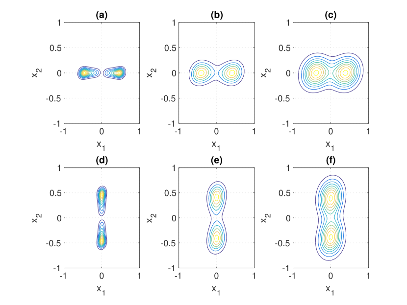
Figure 1: Contour lines of stationary opinion distribution for $\alpha=0.01$ and $\zeta(p,q)$ as in (52). Plots (a), (b), (c): prejudice as in (53). Plots (d), (e), (f): prejudice as in (54). Plots (a), (d): $\sigma_{n}^{2}=10^{-3}$. Plots (b), (e): $\sigma_{n}^{2}=5\times 10^{-3}$; plots (c), (f): $\sigma_{n}^{2}=10^{-2}$.

Next, in Fig. 2 we investigate the effect of topic correlation, as expressed by the coupling matrix ${\bf C}$. We use the same interaction strength as per (52), and the prejudice given in (54). Also, as before, $\alpha(p)=0.01$ and $\sigma_{n}^{2}=10^{-3}$. Finally, we consider the coupling matrix as in (51), with $\rho\in\{-10,-5,0,5,10\}$. For $\rho=0$ there is no interaction between the two opinion components; changing $\rho$ does not have any effect on the mean of the stationary distribution for each personality ((13)), leading to peaks whose locations are essentially invariant with respect to $\rho$. Notice that the distribution of $x_{2}$ is independent of $\rho$. Moreover, due to the symmetric scenario, in all cases the stationary distribution shows a reflectional symmetry around the origin. Finally, changing $\rho$ into $-\rho$ has, in the considered scenario, the effect of reflecting the stationary distribution around the $x_{2}$-axis, or, in other words, of changing $x_{1}$ into $-x_{1}$. From the system point of view, the effect of different correlation values implies a larger share of agents that have strong positive opinions on both subjects (positive correlation value) or one strong positive and one strong negative opinion (negative correlation value). Going back to the previous practical example, agents which are in favor of a low level of taxation will judge more positively or more negatively the government action, depending on the correlation coefficient sign.

Figure 2: Contour lines of stationary opinion distribution for $\alpha=0.01$, $\sigma_{n}^{2}=10^{-3}$, and $\zeta(p,q)$ as in (52). Coupling matrix given by (51). From left to right: $\rho=-10,-5,0,5,10$.

VII-B Community-based scenario, the influence of ${\bf Z}$ and the insurgence of instability

We now assess the impact of the interaction strength matrix ${\bf Z}$ on the stability of opinions. We consider a different scenario, in which there are $M$ personalities ($M$ even), all with the same stubbornness level $\alpha=0.01$, organized in two communities and with an interaction similar to that considered in Example 1, but with $N=2$, i.e.,

$$\underline{{\bf Z}}=\left(\left[\begin{array}[]{cc}\zeta_{1}&-\zeta_{2}\\ -\zeta_{2}&\zeta_{1}\end{array}\right]\otimes\mathbf{1}_{M/2}\right)\otimes{\bf C}$$ (55)

with $\zeta_{1}=1$ and $\zeta_{2}$ used as a parameter. We consider ${\bf C}$ as given by (51) with $\rho=1$, the prejudice as given in (54), and $\sigma_{n}^{2}=10^{-3}$. Also, $\rho_{0}(p)$ is given by (25) with $r_{i}=1/M$ for all $i$. As a possible practical example of such a scenario, we can think of two religious sects, say Bogumils and Cathars, which have generally different views on two topics, represented by the two opinions $x_{1}$ and $x_{2}$.

It is not difficult to show that the stability region boundaries are the same as for Example 1, since ${\bf C}$ is Hurwitz-stable. Furthermore, we can derive the asymptotic expression of the mean in (50) by exploiting Remark 3 in Section V and writing from (7) and (9) $\underline{\bm{\Xi}}=\beta{\bf I}_{M}\otimes{\bf C}$, where $\beta=\bar{\alpha}\frac{1-\zeta_{2}}{2}+\alpha$. If $\beta>0$, through some algebra and by applying the properties of the Kronecker product, we obtain

$${\bf m}(p,\cdot,\infty)=\frac{\alpha}{\alpha-\overline{\alpha}\zeta_{2}}{\bf u}(p).$$ (56)

Thus, if $\zeta_{2}<\alpha/\overline{\alpha}\simeq 0.0101$, the system is stable.

Fig. 3 shows the stationary distribution for increasing value of $\zeta_{2}$. As it can be seen, Bogumils and Cathars merge because of the attractive forces for $\zeta_{2}=-0.2$ or lower, while, for $-0.1<\zeta_{2}<0$, notwithstanding their reciprocal attraction, they remain separated because of the effect of the prejudice. For $0<\zeta_{2}<\alpha/\overline{\alpha}$, the two communities repel each other, but this repulsion is not strong enough to win the effect of prejudice, so stability is preserved while the means grow larger and larger for $\zeta_{2}\uparrow\alpha/\overline{\alpha}$.

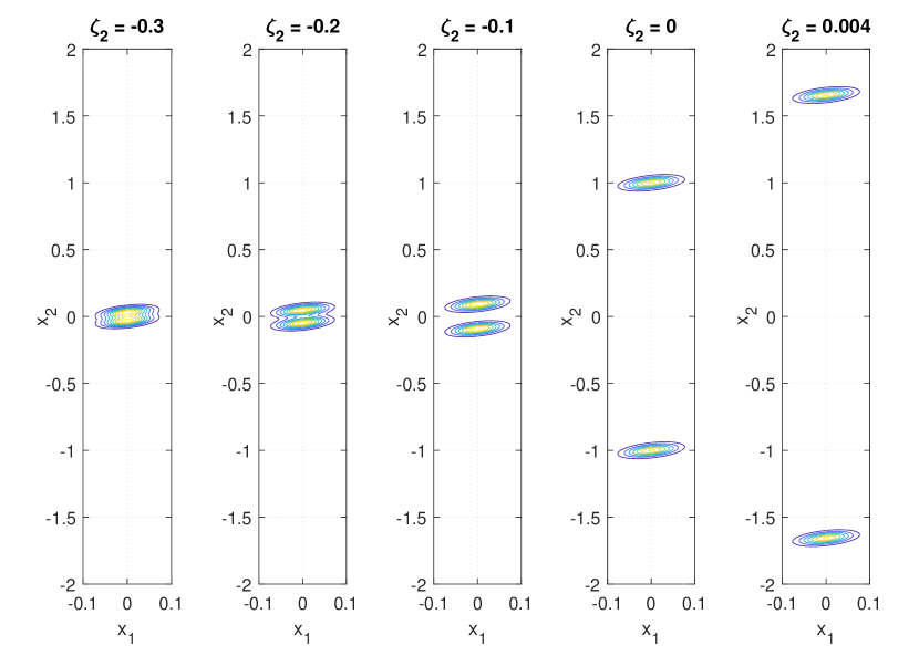
Figure 3: Stationary opinion distribution for $\alpha=0.01$, $\sigma_{n}^{2}=10^{-3}$, ${\bf Z}$ as in (55) ($\zeta_{1}=1$), for several values of $\zeta_{2}$ in the stability region. Coupling matrix given by (51) with $\rho=1$. From left to right: $\zeta_{2}=-0.3,-0.2,-0.1,0,0.004$.

For $\zeta_{2}>\alpha/\overline{\alpha}$, the system is not stable anymore, and (56) does not hold. In particular, when $\zeta_{2}<\zeta_{1}+2\alpha/\overline{\alpha}=1.0202$, the intra-community attraction and the inter-community repulsion have such a relative strength that the system experiences type-II instability: the communities are preserved but their respective means tend to diverge. In our example, the two religious sects are so enemy of each other, to radicalize their views while retaining a strong identity within themselves, giving rise to religious fanaticism. We now look at the time evolution of opinions in the case where, for all personalities, opinions start deterministically from the origin. Fig. 4 shows the opinions at time instants $t=5,10,15,20$, for $\zeta_{2}=0.1$. Notice that, because of the correlation, the two communities diverge along the bisector of the I-III quadrants.

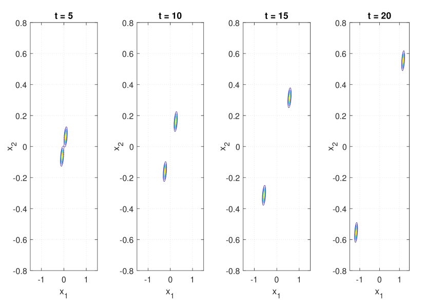
Figure 4: Contour lines of opinion distribution for $\alpha=0.01$, $\sigma_{n}^{2}=10^{-3}$, ${\bf Z}$ as in (55) ($\zeta_{1}=1$, $\zeta_{2}=0.1$). Coupling matrix given by (51) with $\rho=1$. From left to right: $t=5,10,15,20$.

Finally, for $\zeta_{2}>\zeta_{1}+2\alpha/\overline{\alpha}$, the inter-community repulsion prevails on intra-community attraction, the system experiences type-I instability, and the variance within the two communities also grows to infinity. In other words, Bogumils and Cathars dissolve themselves into heterogeneous crowds not having definite views on the two topics of interest. Fig. 4 shows the opinions at time instants $t=0.15,0.3,0.45,0.5$ for $\zeta_{2}=10$, again when the opinions all start deterministically from the origin. The dynamic is similar, but faster than in the previous case, and the communities expand, so that, for $t$ sufficiently large, their boundaries disappear.

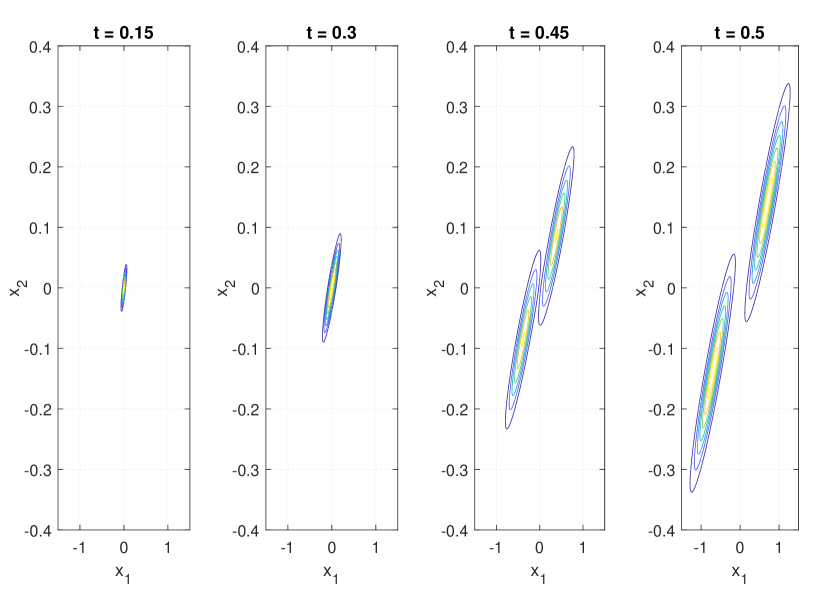
Figure 5: Contour lines of opinion distribution for $\alpha=0.01$, $\sigma_{n}^{2}=10^{-3}$, ${\bf Z}$ as in (55) ($\zeta_{1}=1$, $\zeta_{2}=10$). Coupling matrix given by (51) with $\rho=1$. From left to right: $t=0.15,0.3,0.45,0.5$.

VII-B1 Finite-network behavior

In order to assess the validity of the mean-field approach, in Fig. 6 we show the opinion distribution behavior for a finite set of $U=500$ agents, by solving numerically (3). In particular, we consider the same model as in Figs. 3-4 for $\zeta_{2}\in\{-0.1,0,0.004,0.1\}$. The first half of the agents are Bogumils, while the others are Cathars. For the first three values of $\zeta_{2}$, which correspond to a stable system, we show the stationary opinion distribution. For $\zeta_{2}=0.1$, we show the distribution at time $t=20$. As it can be seen, the results in Figs. 3-4 match those in Fig. 6, indicating that the asymptotic analysis well represents the opinion dynamics of relatively small populations.

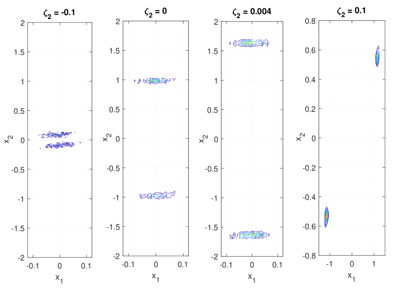
Figure 6: Contour lines of simulated opinion distribution for $U=500$, $\alpha=0.01$, $\sigma_{n}^{2}=10^{-3}$, ${\bf Z}$ as in (55) ($\zeta_{1}=1$), where the first half of users belong to community 1, while the second half to community 2. Coupling matrix given by (51) with $\rho=1$. From left to right: $\zeta_{2}=-0.1,0,0.004,0.1$. For the rightmost graph, $t=20$.

VII-C Rotational effects

We now consider the case in which the dynamics is stable in both dimensions, but the effect of the coupling matrix yields instability (of Type I). Consider again the two-community scenario given by (55), but with $\zeta_{1}=1$ and $\zeta_{2}=-0.1$. Note that, in the scalar case, this would be a stable scenario. However, let us now consider a coupling matrix given by

$${\bf C}=\left[\begin{array}[]{cc}0&1\\ -1&0\end{array}\right]$$ (57)

which is easily seen to have eigenvalues equal to $\pm j$. This is quite an artificial scenario, since this coupling matrix has rather an ad-hoc shape, to which it is difficult to associate any real-world situation. All the other parameters are the same as in the previous example, except for the prejudice, which is given by

$${\bf u}(p)=\left\{\begin{array}[]{cc}[0,-10],&p<0\\ {[0,10]},&p\geq 0\,.\end{array}\right.$$ (58)

It is easy to see that, for the $i$-th discrete personality, the covariance matrix in (12) is given by:

$$\bm{\Sigma}\left(p_{i},t\right)=\sigma^{2}_{n}t{\bf I}_{2}$$ (59)

independently from $i$. Note that such covariance matrix does not reach any finite limit for $t\rightarrow\infty$, hence the system is unstable. Fig. 7 shows the temporal evolution of the opinion distribution, for $t=1,10,20,30,40,50,60,70,80$. The peaks corresponding to the two communities widen along time, as expected, while their means undergo a rotation around the origin, at some instants (such as at $t=60$) making the peaks temporarily merge.

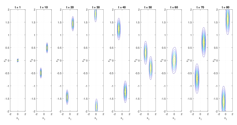
Figure 7: Contour lines of opinion distribution for $\alpha=0.01$, $\sigma_{n}^{2}=10^{-3}$, ${\bf Z}$ as in (55) ($\zeta_{1}=1$, $\zeta_{2}=-0.1$). Coupling matrix given by (57). From left to right: $t=1,10,20,30,40,50,60,70,80$.

VIII Conclusions

Several analytical models representing the dynamics of social opinions have been proposed in the literature. By drawing on this body of work, we developed a model that accounts for the individual endogenous process of opinion evolution as well as for the possible adversarial behavior of individuals. Importantly, our model also represents the interdependence between opinions on different, yet correlated, subjects. Under asymptotic conditions on the size of the individuals’ population, we obtained the time evolution of the opinions distribution as the solution of a multidimensional Fokker-Planck equation. We then discussed the stability conditions and derived the steady-state solution. Our numerical results match the stability conditions we obtained and show interesting phenomena in collective belief dynamics.

Appendix A Derivation of (11)

By using (II-A) and by neglecting dependencies on the system variables unless strictly necessary, we can rewrite the FP equation in (II-A) as:

$$\frac{\partial}{\partial t}\rho({\bf x}) = \sum_{n=1}^{N}\frac{\partial}{\partial x_{n}}\left[({\bf e}_{n}^{\mathsf{T}}\bm{\Xi}{\bf x}-\phi_{n}\rho({\bf x})\right]+\frac{1}{2}\sum_{m,n=1}^{N}D_{mn}\frac{\partial^{2}}{\partial x_{m}\partial x_{n}}\rho({\bf x})$$ (60)

where ${\bf e}_{n}$ is the vector with all zero components but the $n$-th one equal to 1. Then, by taking the Fourier transform of (60) with respect to ${\bf x}$, we obtain

$$\frac{\partial}{\partial t}\widehat{\rho}(\bm{\nu})+\bm{\nu}^{\mathsf{T}}\bm{\Xi}\nabla_{\bm{\nu}}\widehat{\rho}(\bm{\nu})=-\left[j2\pi\bm{\nu}^{\mathsf{T}}\bm{\phi}+2\pi^{2}\bm{\nu}^{\mathsf{T}}{\bf D}\bm{\nu}\right]\widehat{\rho}(\bm{\nu})$$ (61)

where $\bm{\nu}$ is the variable in the transformed domain, while $\hat{f}(\bm{\nu})$ is the Fourier transform of the generic function $f({\bf x})$. The operator $\nabla_{\bm{\nu}}$ is the gradient with respect to the vector $\bm{\nu}$. Next we transform the above first-order partial-derivative equation into a system of first-order ordinary differential equations by using the method of characteristics [37]. To this end we introduce an auxiliary parameter $u$ and consider $t=t(u)$, $\bm{\nu}=\bm{\nu}(u)$ and $\widehat{\rho}(p,\bm{\nu}(u),t(u))=\widehat{\rho}(u)$, with initial conditions $t(0)=0$, $\bm{\nu}(0)=\bm{\nu}_{0}$ and $\widehat{\rho}(p,\bm{\nu}(0),t(0))=\widehat{\rho}_{0}(p,\bm{\nu}_{0})=\widehat{\rho}(0)$. According to the rule of total derivative, $\frac{{\rm\,d}\widehat{\rho}}{{\rm\,d}u}$ can be written as

$$\frac{{\rm\,d}\widehat{\rho}}{{\rm\,d}u}=\frac{\partial\widehat{\rho}}{\partial t}\frac{{\rm\,d}t}{{\rm\,d}u}+\frac{{\rm\,d}\bm{\nu}^{\mathsf{T}}}{{\rm\,d}u}\nabla_{\bm{\nu}}\widehat{\rho}\,.$$

If we set $\frac{{\rm\,d}t}{{\rm\,d}u}=1$ and $\frac{{\rm\,d}\bm{\nu}}{{\rm\,d}u}=\bm{\Xi}^{\mathsf{T}}\bm{\nu}$, the above total derivative corresponds to the left hand side of (61). With such setting we can reduce (61) to the following system of differential equations:

$$\left\{\begin{array}[]{ccl}\frac{{\rm\,d}t}{{\rm\,d}u}&=&1\\ \frac{{\rm\,d}\bm{\nu}}{{\rm\,d}u}&=&\bm{\Xi}^{\mathsf{T}}\bm{\nu}\\ \frac{{\rm\,d}\widehat{\rho}}{{\rm\,d}u}&=&-\left[j2\pi\bm{\nu}^{\mathsf{T}}\bm{\phi}+2\pi^{2}\bm{\nu}^{\mathsf{T}}{\bf D}\bm{\nu}\right]\widehat{\rho}\,.\end{array}\right.$$ (62)

The first two equations are easily solved as $t(u)=u$, and $\bm{\nu}(u)={\rm e}^{\bm{\Xi}^{\mathsf{T}}u}\bm{\nu}_{0}$. By substituting these solutions in the third equation, the latter can be rearranged as

$$\frac{{\rm\,d}\widehat{\rho}(u)}{\widehat{\rho}(u)}=-\left[j2\pi\bm{\nu}_{0}^{\mathsf{T}}{\rm e}^{\bm{\Xi}u}\bm{\phi}+2\pi^{2}\bm{\nu}_{0}^{\mathsf{T}}{\rm e}^{\bm{\Xi}u}{\bf D}{\rm e}^{\bm{\Xi}^{\mathsf{T}}u}\bm{\nu}_{0}\right]{\rm\,d}u$$ (63)

We now recall that $\bm{\phi}=\bm{\phi}(t)$ is a function of $t$. Since $t=u$, by integrating with respect to $u$ the above equation, we get

$$\log\frac{\widehat{\rho}(u)}{\widehat{\rho}(0)}=-j2\pi\bm{\nu}_{0}^{\mathsf{T}}\int_{0}^{u}{\rm e}^{\bm{\Xi}w}\bm{\phi}(w){\rm\,d}w-2\pi^{2}\bm{\nu}_{0}^{\mathsf{T}}\left(\int_{0}^{u}{\rm e}^{\bm{\Xi}w}{\bf D}{\rm e}^{\bm{\Xi}^{\mathsf{T}}w}{\rm\,d}w\right)\bm{\nu}_{0}$$ (64)

The solution for $\hat{\rho}(u)$ is given by

$$\widehat{\rho}(u) = \widehat{\rho}(0)\exp\left\{-j2\pi\bm{\nu}_{0}^{\mathsf{T}}\int_{0}^{u}{\rm e}^{\bm{\Xi}w}\bm{\phi}(w){\rm\,d}w-2\pi^{2}\bm{\nu}_{0}^{\mathsf{T}}\left(\int_{0}^{u}{\rm e}^{\bm{\Xi}w}{\bf D}{\rm e}^{\bm{\Xi}^{\mathsf{T}}w}{\rm\,d}w\right)\bm{\nu}_{0}\right\}$$ (65)

By substituting $u=t$ and $\bm{\nu}_{0}={\rm e}^{-\bm{\Xi}^{\mathsf{T}}t}\bm{\nu}(t)$ into (65), and after reintroducing all dependencies we finally obtain

$$\widehat{\rho}(p,\bm{\nu},t) = \widehat{\rho}_{0}(p,\bm{\nu}_{0})\exp\left\{-j2\pi\bm{\nu}^{\mathsf{T}}\underbrace{{\rm e}^{-\bm{\Xi}(p)t}\left[\int_{0}^{t}{\rm e}^{\bm{\Xi}(p)\tau}\bm{\phi}(p,\tau){\rm\,d}\tau\right]}_{\widetilde{{\bf m}}(p,t)}-2\pi^{2}\bm{\nu}^{\mathsf{T}}\underbrace{\left(\int_{0}^{t}{\rm e}^{-\bm{\Xi}(p)\tau}{\bf D}{\rm e}^{-\bm{\Xi}(p)^{\mathsf{T}}\tau}{\rm\,d}\tau\right)}_{\bm{\Sigma}(p,t)}\bm{\nu}\right\}$$ (66)

$$= \widehat{\rho}_{0}\left(p,\bm{\nu}{\rm e}^{-\bm{\Xi}(p)t}\right)\exp\left\{-j2\pi\bm{\nu}^{\mathsf{T}}\widetilde{{\bf m}}(p,t)-2\pi^{2}\bm{\nu}^{\mathsf{T}}\bm{\Sigma}(p,t)\bm{\nu}\right\}$$

where we used the fact that

$$\bm{\nu}_{0}^{\mathsf{T}}\left(\int_{0}^{t}{\rm e}^{\bm{\Xi}w}{\bf D}{\rm e}^{\bm{\Xi}^{\mathsf{T}}w}{\rm\,d}w\right)\bm{\nu}_{0} = \bm{\nu}^{\mathsf{T}}\left(\int_{0}^{t}{\rm e}^{-\bm{\Xi}(p)t}{\rm e}^{\bm{\Xi}w}{\bf D}{\rm e}^{\bm{\Xi}^{\mathsf{T}}w}{\rm e}^{-\bm{\Xi}(p)t}{\rm\,d}w\right)\bm{\nu}$$ (67)

$$= \bm{\nu}^{\mathsf{T}}\left(\int_{0}^{t}{\rm e}^{\bm{\Xi}(w-t)}{\bf D}{\rm e}^{\bm{\Xi}^{\mathsf{T}}(w-t)}{\rm\,d}w\right)\bm{\nu}$$

$$\stackrel{{\scriptstyle(a)}}{{=}} \bm{\nu}^{\mathsf{T}}\left(\int_{0}^{t}{\rm e}^{-\bm{\Xi}\tau}{\bf D}{\rm e}^{-\bm{\Xi}^{\mathsf{T}}\tau}{\rm\,d}\tau\right)\bm{\nu}$$

and in $(a)$ we defined $\tau=t-w$. Now, by taking the inverse Fourier transform w.r.t. $\bm{\nu}$ of (66), we get

$$\rho(p,{\bf x},t)={\rm e}^{\bm{\Xi}(p)t}\rho_{0}\left(p,{\bf x}{\rm e}^{\bm{\Xi}(p)t}\right)\star{\cal G}\left({\bf x},\widetilde{{\bf m}}(p,t),\bm{\Sigma}(p,t)\right)$$ (68)

where the symbol $\star$ represents the convolution operator and ${\cal G}\left({\bf x},\widetilde{{\bf m}}(p,t),\bm{\Sigma}(p,t)\right)$ is the pdf of the multivariate Gaussian distribution with mean $\widetilde{{\bf m}}(p,t)$ and covariance $\bm{\Sigma}(p,t)$. Finally, after a suitable change of variable, and by recalling that $\rho_{0}(p,{\bf y})=\rho_{0}({\bf y}|p)\rho_{0}(p)$, we rewrite the convolution product in (68) as

$$\rho(p,{\bf x},t) = \rho_{0}(p)\int_{{\bf y}}\rho_{0}({\bf y}|p)\,{\cal G}\left({\bf x},{\bf m}(p,{\bf y},t),\bm{\Sigma}(p,t)\right){\rm\,d}^{N}{\bf y}$$ (69)

where ${\bf m}(p,{\bf y},t)\triangleq{\rm e}^{-\bm{\Xi}(p)t}{\bf y}+\widetilde{{\bf m}}(p,t)={\rm e}^{-\bm{\Xi}(p)t}\left[{\bf y}+\int_{0}^{t}{\rm e}^{\bm{\Xi}(p)\tau}\bm{\phi}(p,\tau){\rm\,d}\tau\right]$.

Appendix B Proof of Theorem 2

B-A Preliminaries

Under steady state conditions, using (42) and the definition of ${\bf f}(p)$, we can rewrite $\bm{\beta}(p)$ as

$$\bm{\beta}(p) = \int_{q}\zeta(p,q)\rho_{0}(q)\int_{{\bf x}}\frac{{\bf x}}{\sqrt{2\pi|{\bf W}(q)|}}{\rm e}^{-\frac{1}{2}({\bf x}-{\bf f}(q))^{\mathsf{T}}{\bf W}(q)^{-1}({\bf x}-{\bf f}(q))}{\rm\,d}^{N}{\bf x}{\rm\,d}q$$ (70)

$$= \int_{q}\zeta(p,q)\rho_{0}(q){\bf f}(q){\rm\,d}q$$

By changing variable and considering $\bm{\phi}(p)=\frac{\bm{\beta}(p)}{\eta(p)}$, we rewrite the above expression as

$$\bm{\phi}(p) = \underbrace{\int_{q}\frac{\zeta(p,q)\alpha(q){\bf u}(q)\rho_{0}(q)}{\eta(p)w(q)}{\rm\,d}q}_{{\bf h}(q)}+\int_{q}\underbrace{\frac{\zeta(p,q)\bar{\alpha}(q)\eta(q)}{\eta(p)w(q)}}_{\Phi(p,q)}\bm{\phi}(q)\rho_{0}(q){\rm\,d}q$$ (71)

$$= {\bf h}(p)+\int_{q}\Phi(p,q)\bm{\phi}(q)\rho_{0}(q){\rm\,d}q$$

which is the Fredholm equation of the second type [38]. In the following, we will consider a per-element solution of the above equation.

In order to solve the Fredholm equation, let us denote by ${\cal A}[\phi](p)$ the following operator

$${\cal A}[\phi](p)=\int_{p}\Phi(p,q)\phi(q)\rho_{0}(q){\rm\,d}q$$ (72)

operating on a Banach space of Lipschits continuous functions $\phi(q)$, where $\phi(q)$ is the generic component of $\bm{\phi}(p)$. We have that $\phi(p)$ is equipped with the following norm:

$$\|\phi(p)\|_{\rm Lip} = c_{0}\sup_{{\cal P}}|\phi(p)|+c_{1}\sup_{p,q\in{\cal P},p\neq q}\frac{|\phi(p)-\phi(q)|}{|p-q|}$$ (73)

$$= c_{0}\|\phi(p)\|_{\infty}+c_{1}\|\phi(p)\|_{\rm L}$$

with $c_{0},c_{1}>0$ and $c_{0}+c_{1}=1$. Then we can rewrite (71) as

$$\phi(p)=h(p)+{\cal A}[\phi](p)$$

where $h(p)$ is the generic component of ${\bf h}(p)$. From the above expression, we get

$$\phi(p)=({\cal I}-{\cal A})^{-1}[h](p)$$

whenever $({\cal I}-{\cal A})^{-1}[\cdot]$ exists and is continuous over the aforementioned Banach space.

Now let $R(p)$, $R:{\cal P}\to[0,1]$ be a continuous initial cumulative distribution with pdf $\rho_{0}(p)$, and let $R_{n}(p)$ be the stepwise approximation of $R(p)$ with meshsize equal to $1/n$. Then, using (72), we can write

$${\cal A}_{n}[\phi]=\int_{\cal P}\Phi(p,q)\phi(q){\rm\,d}R_{n}(q),\quad{\cal A}[\phi]=\int_{\cal P}\Phi(p,q)\phi(q){\rm\,d}R(q),$$

and

$$h_{n}(p)=\int_{{\cal P}}\frac{\zeta(p,q)\alpha(q)u(q)}{\eta(p)w(q)}{\rm\,d}R_{n}(q),\quad h(p)=\int_{{\cal P}}\frac{\zeta(p,q)\alpha(q)u(q)}{\eta(p)w(q)}{\rm\,d}R(q),$$

Given the above definitions, we introduce $\phi_{n}(p)$ as

$$\phi_{n}(p)=\left({\cal I}-{\cal A}_{n}\right)^{-1}[h_{n}](p)\,.$$

B-B Main Theorem

We can now prove Theorem 2 whose statement is reported again below for completeness:

Theorem 3

i) The Fredholm equation (71) admits a unique solution which is Lipschitz-continuous. ii) The solution $\phi(p)$ of the Fredholm equation (71), under any distribution $\rho_{0}(p)$, which is continuous at every point in $p$, is the uniform limit of solutions $\phi_{n}(p)$, obtained by replacing distribution $\rho_{0}(p)$ with its discrete approximation $\rho_{n}(p)$ whose mesh-size is $\frac{1}{n}$.

Proof:

In order to prove the thesis we proceed as follows:

• i) descends from the properties of operator ${\cal A}[\cdot]$ over the Banach space of Lipschitz-continuous functions equipped with norm $\|\cdot\|_{\rm Lip}$, which satisfies $\|{\cal A}[\cdot]\|_{\rm Lip}<1$, since we can derive the existence and the continuity of the operator $({\cal I}-{\cal A})^{-1}[\cdot]$ with respect to norm $\|\cdot\|_{\rm Lip}$ (see Lemma 1 below).

• ii) descends from Lemma 2 which shows that operators ${\cal A}_{n}[\cdot]$ converge to the operator ${\cal A}[\cdot]$, and from Lemma 3 which shows that convergence holds also for the inverse operators $({\cal I}-{\cal A}_{n})^{-1}[\cdot]$. Then, using Lemma 4, we show that $\phi_{n}(p)=({\cal I}-{\cal A}_{n})^{-1}[h_{n}](p)$ converges to $\phi(p)=({\cal I}-{\cal A})^{-1}[h](p)$.

∎

Lemma 1

Given the operator ${\cal A}[\cdot]$ defined above we have that $\|{\cal A}[\phi](p)\|_{\mathrm{Lip}}<1$ for opportunely chosen $c_{0}$ and $c_{1}$ under the assumption that $\Phi(p,q)$ is $C^{1}({\cal P}^{2})$. Furthermore the operator $({\cal I}-{\cal A})^{-1}[\cdot]$ exists continuous with respect to norm $\|\cdot\|_{\rm Lip}$.

Proof:

We have that

$$|{\cal A}[\phi](p)| \leq \int_{q}\left|\Phi(p,q)\phi(q)\rho_{0}(q){\rm\,d}q\right|\leq\int_{q}|\Phi(p,q)\rho_{0}(q)||\phi(q)|{\rm\,d}q$$ (74)

$$\leq \|\phi(p)\|_{\infty}\int_{q}|\Phi(p,q)\rho_{0}(q)|{\rm\,d}q$$

Therefore, by assuming that $\alpha(p)$ and $\zeta(p,p^{\prime})$ are regular in their argmmuments, we have

$$\|{\cal A}[\phi](p)\|_{\infty} = \sup_{p}\|{\cal A}[\phi](p)\|$$ (75)

$$\leq \|\phi(p)\|_{\infty}\sup_{p}\int_{q}\Phi(p,q)\rho_{0}(q){\rm\,d}q$$

$$\leq \|\phi(p)\|_{\infty}\frac{1}{\eta(p)}\sup_{q}\frac{\bar{\alpha}(q)\eta(q)}{\alpha(q)+\bar{\alpha}(q)\eta(q)}\underbrace{\int_{q}\zeta(p,q)\rho_{0}(q){\rm\,d}q}_{\eta(p)}$$

$$= \|\phi(p)\|_{\infty}\sup_{q}\frac{\bar{\alpha}(q)\eta(q)}{\alpha(q)+\bar{\alpha}(q)\eta(q)}$$

$$= \kappa\|\phi(p)\|_{\infty}$$

where $\kappa<1$. Similarly, using the Lagrange theorem, we have

$$\sup_{p,q\in{\cal P},p\neq q}\frac{|y(p)-y(q)|}{|p-q|}=\sup_{p}\left|\frac{{\rm\,d}y(p)}{{\rm\,d}p}\right|$$

for any continuous and differentiable function $y(p)$. Therefore,

$$\left|\frac{{\rm\,d}{\cal A}[\phi](p)}{{\rm\,d}p}\right| = \left|\int_{q}\frac{\partial\Phi(p,q)}{\partial p}\phi(q)\rho_{0}(q){\rm\,d}q\right|\leq$$ (76)

$$\leq \int_{q}\left|\frac{\partial\Phi(p,q)}{\partial p}\phi(q)\rho_{0}(q)\right|{\rm\,d}q$$

$$\leq \left|\sup_{p,q\in{\cal P}}\frac{\partial\Phi(p,q)}{\partial p}\rho_{0}(q)\right|\|\phi(q)\|_{\infty}$$

$$= \|\Psi(p,q)\|_{L}\|\phi(q)\|_{\infty}$$

Note that, to obtain the last expression, we defined $\|\Psi(p,q)\|_{\rm L}=\sup_{p,q\in{\cal P}}\left|\frac{\partial\Phi(p,q)}{\partial p}\rho_{0}(q)\right|$. Now combining (75) and (76), we have:

$$\|{\cal A}[\phi](p)\|_{\rm Lip}\leq c_{0}\kappa{\|\phi(p)\|_{\infty}}+c_{1}\|\Psi(p,q)\|_{\rm L}\|\phi(p)\|_{\infty}$$

Dividing both sides by $\|\phi(p)\|_{\rm Lip}$ we get

$$\frac{\|{\cal A}[\phi](p)\|_{\rm Lip}}{\|\phi(p)\|_{\rm Lip}}\leq c_{0}\frac{\kappa{\|\phi(p)\|_{\infty}}}{\|\phi(p)\|_{\rm Lip}}+c_{1}\|\Psi(p,q)\|_{\rm L}\frac{\|\phi(p)\|_{\infty}}{\|\phi(p)\|_{\rm Lip}}.$$

Now, since by construction $\frac{\|\phi(p)\|_{\infty}}{\|\phi(p)\|_{\rm Lip}}\leq\frac{1}{c_{0}}$, we have

$$\|{\cal A}[\phi](p)\|_{\rm Lip}=\sup\frac{\|{\cal A}[\phi](p)\|_{\rm Lip}}{\|\phi(p)\|_{\rm Lip}}\leq\kappa+\frac{c_{1}}{c_{0}}\|\Psi(p,q)\|_{\rm L}$$

which can be made smaller than 1 by opportunely setting $c_{0}$ and $c_{1}$, i.e. by setting $\frac{c_{1}}{c_{0}}<\frac{1-\kappa}{\|\Psi(p,q)\|_{\rm L}}$.

For a generic linear operator ${\cal A}[\cdot]$ defined over a Banach space such that $\|{\cal A}[\cdot]\|<1$, the associated operator $({\cal I}-{\cal A})^{-1}[\cdot]$ exists continuous and can be written as [38, Th. 8 p. 102 and Th. 1 p. 111]

$$({\cal I}-{\cal A})^{-1}[\cdot]=\sum_{k=0}^{\infty}({\cal A})^{k}[\cdot]\,.$$ (77)

∎

We now consider the sequence of pertubated operators ${\cal A}_{n}[\cdot]$. The general result below applies.

Lemma 2

Given a sequence of operators ${\cal A}_{n}[\cdot]$ and a sequence of functions $h_{n}(p)$ as defined above, they converge to, respectively, the above expressions of ${\cal A}[\cdot]$ and $h(p)$ in Lipschitz norm (i.e., $\|{\cal A}_{n}[\cdot]-{\cal A}[\cdot]\|_{\mathrm{Lip}}\to 0$ and $\|h_{n}(p)-h(p)\|_{\mathrm{Lip}}\to 0$).

Proof:

To simplify the notation, without loss of generality we assume ${\cal P}=[0,1]$ (we recall that ${\cal P}$ is assumed to be compact). Then,

$${\cal A}_{n}[\phi(p)]=\int_{\cal P}\Phi(p,q)\phi(q){\rm\,d}R_{n}(q) = \sum_{m=0}^{n-1}\Phi\left(p,\frac{m}{n}\right)\phi\left(\frac{m}{n}\right)\int_{\frac{m}{n}}^{\frac{m+1}{n}}{\rm\,d}R(q)$$

Furthermore,

$$|{\cal A}[\phi(p)]-{\cal A}_{n}[\phi(p)]|=\sum_{m=0}^{n-1}\int_{\frac{m}{n}}^{\frac{m+1}{n}}\left[\Phi(p,q)\phi(q)-\Phi\left(p,\frac{m}{n}\right)\phi\left(\frac{m}{n}\right)\right]{\rm\,d}R(q)$$

We therefore obtain:

$$|{\cal A}[\phi(p)]-{\cal A}_{n}[\phi(p)]| \leq \sum_{m=0}^{n-1}\int_{\frac{m}{n}}^{\frac{m+1}{n}}\left|\Phi(p,q)\right|\left|\phi(q)-\phi\left(\frac{m}{n}\right)\right|{\rm\,d}R(q)$$

$$+ \sum_{m=0}^{n-1}\int_{\frac{m}{n}}^{\frac{m+1}{n}}\left|\Phi(p,q)-\Phi\left(p,\frac{m}{n}\right)\right|\left|\phi\left(\frac{m}{n}\right)\right|{\rm\,d}R(q)$$

$$\leq \|\Phi(p,q)\|_{\infty}\frac{\|\phi(p)\|_{L}}{n}\int_{0}^{1}{\rm\,d}R(q)$$

$$+ \frac{\|\Phi(p,q)\|_{\rm L}}{n}\|\phi(p)\|_{\infty}\int_{0}^{1}{\rm\,d}R(q)$$

$$= \frac{1}{n}\left(\|\Phi(p,q)\|_{\infty}\|\phi(p)\|_{L}+\|\Phi(p,q)\|_{L}\|\phi(p)\|_{\infty}\right)$$

It follows that:

$$\|{\cal A}[\phi(p)]-{\cal A}_{n}[\phi(p)]\|_{\infty}\leq\frac{1}{n}\left(\|\Phi(p,q)\|_{\infty}\|\phi(p)\|_{L}+\|\Phi(p,q)\|_{L}\|\phi(p)\|_{\infty}\right)$$

Similarly, since $\Phi(p,p^{\prime})$ is assumed to be differentiable with continuous derivative with respect to $p$ and $q$, both ${\cal A}[\phi(p)]$ and ${\cal A}_{n}[\phi(p)]$ are differentiable at every point with continuous derivative and:

$$\left|\frac{{\rm\,d}{\cal A}[\phi(p)]}{{\rm\,d}p}-\frac{{\rm\,d}{\cal A}_{n}[\phi(p)]}{{\rm\,d}p}\right| = \left|\sum_{m=0}^{n-1}\int_{\frac{m}{n}}^{\frac{m+1}{n}}\left[\frac{\partial\Phi(p,q)}{\partial p}\phi(q)-\frac{\partial\Phi\left(p,\frac{m}{n}\right)}{\partial p}\phi\left(\frac{m}{n}\right)\right]{\rm\,d}R(q)\right|$$

Proceeding as before, we get:

$$\|{\cal A}[\phi(p)]-{\cal A}_{n}[\phi(p)]\|_{L} \leq \frac{1}{n}\left(\left\|\frac{\partial\Phi(p,q)}{\partial p}\right\|_{\infty}\|\phi(p)\|_{L}+\left\|\frac{\partial\Phi(p,q)}{\partial p}\right\|_{L}\|\phi(p)\|_{\infty}\right)$$

and

$$\|{\cal A}[\phi(p)]-{\cal A}_{n}[\phi(p)]\|_{\mathrm{Lip}} \leq \frac{c_{0}}{n}\left(\|\Phi(p,q)\|_{\infty}\|\phi(p)\|_{L}+\Phi(p,q)\|_{L}\|\phi(p)\|_{\infty}\right)$$

$$+\frac{c_{1}}{n}\left(\left\|\frac{\partial\Phi(p,q)}{\partial p}\right\|_{\infty}\|\phi(p)\|_{L}+\left\|\frac{\partial\Phi(p,q)}{\partial p}\right\|_{L}\|\phi(p)\|_{\infty}\right)$$

Since in the right hand side of the above expressions none of the norms depend on $n$, it easy to see that $\|{\cal A}[\phi(p)]-{\cal A}_{n}[\phi(p)]\|_{\mathrm{Lip}}\to 0$ as $n\to\infty$. With similar arguments, we can prove that $\|h(p)-h_{n}(p)\|_{\mathrm{Lip}}\to 0$ as $n\to\infty$. ∎

Lemma 3

Given a Banach space with norm $\|\cdot\|$, and a sequence of linear operators ${\cal A}_{n}[\cdot]\to{\cal A}[\cdot]$ in norm, with $\|{\cal A}[\cdot]\|<1$, we have that the continuous operators $({\cal I}[\cdot]-{\cal A}_{n}[\cdot])^{-1}\to({\cal I}[\cdot]-{\cal A}[\cdot])^{-1}$ in norm.

Proof:

Given that $\|{\cal A}[\cdot]\|<1$ by the continuity of norm $\|{\cal A}_{n}[\cdot]\|\to\|{\cal A}[\cdot]\|<1$, for $n$ sufficiently large we can assume $\|{\cal A}_{n}[\cdot]\|<1$. For any of such $n$, we define ${\cal B}_{n}[\cdot]=({\cal I}[\cdot]-{\cal A}_{n}[\cdot])^{-1}-({\cal I}[\cdot]-{\cal A}[\cdot])^{-1}$. By (77), we can write

$${\cal B}_{n}[\cdot]=\sum_{k=0}^{\infty}({\cal A}_{n}[\cdot])^{k}-\sum_{k}({\cal A}[\cdot])^{k}\,.$$

Since both series on the right hand side of the above expression converge, we can write:

$${\cal B}_{n}[\cdot]=\sum_{k=0}^{\infty}({\cal A}_{n}[\cdot])^{k}-({\cal A}[\cdot])^{k}$$

Now, we have:

$$\|{\cal B}_{n}[\cdot]\|=\left\|\sum_{k=0}^{\infty}({\cal A}_{n}[\cdot])^{k}-({\cal A}[\cdot])^{k}\right\|\leq\sum_{k=0}^{\infty}\|({\cal A}_{n}[\cdot])^{k}-({\cal A}[\cdot])^{k}\|$$

where the last inequality follows by the sub-additivity and continuity of the norm.

Denoted with $c_{k}=\|({\cal A}_{n}[\cdot])^{k}-({\cal A}[\cdot])^{k}\|=\|[({\cal A}_{n}[\cdot]-{\cal A}[\cdot])+{\cal A}[\cdot]]^{k}-({\cal A}[\cdot])^{k}\|$, and considering that the operator algebra is, in general, non-commutative, we have:

$$c_{k} = \left\|\sum_{\begin{subarray}{c}x_{i}\in\{0,1\},i=1,\ldots,k\end{subarray}}\prod_{i}({\cal A}[\cdot])^{x_{i}}({\cal A}_{n}[\cdot]-{\cal A}[\cdot])^{1-x_{i}}-({\cal A}[\cdot])^{k}\right\|$$

$$= \left\|\sum_{\begin{subarray}{c}x_{i}\in\{0,1\},i=1,\ldots,k\\ \{x_{1},x_{2}\cdots x_{k}\}\neq\{1,1,\cdots,1\}\end{subarray}}\prod_{i}({\cal A}[\cdot])^{x_{i}}({\cal A}_{n}[\cdot]-{\cal A}[\cdot])^{1-x_{i}}\right\|$$

$$\leq \sum_{\begin{subarray}{c}x_{i}\in\{0,1\},i=1,\ldots,k\\ \{x_{1},x_{2}\cdots x_{k}\}\neq\{1,1,\cdots,1\}\end{subarray}}\prod_{i}\|({\cal A}[\cdot])^{x_{i}}\|\|({\cal A}_{n}[\cdot]-{\cal A}[\cdot])^{1-x_{i}}\|$$

$$= \sum_{i=1}^{k}{k\choose i}\|{\cal A}_{n}[\cdot]-{\cal A}[\cdot]\|^{i}\|{\cal A}[\cdot]\|^{k-i}$$

$$= \sum_{i=1}^{k}{k\choose i}\|{\cal A}[\cdot]\|^{i}\|{\cal A}_{n}[\cdot]-{\cal A}[\cdot]\|^{k-i}$$

$$= (\|{\cal A}[\cdot]\|+\|{\cal A}_{n}[\cdot]-{\cal A}[\cdot]\|)^{k}-\|{\cal A}[\cdot]\|^{k}\,.$$

Therefore, by monotonicity of positive series, we have:

$$\|{\cal B}_{n}[\cdot]\|\leq\sum_{k=0}^{\infty}c_{k}\leq\sum_{k=0}^{\infty}(\|{\cal A}[\cdot]\|+\|{\cal A}_{n}[\cdot]-{\cal A}[\cdot]\|)^{k}-\|{\cal A}[\cdot]\|^{k}$$ (78)

Since $\|{\cal A}_{n}[\cdot]-{\cal A}[\cdot]\|_{\infty}\to 0$ and $\|{\cal A}[\cdot]\|_{\infty}<1$, we can assume $n$ sufficiently large so that $\|{\cal A}[\cdot]\|+\|{\cal A}_{n}[\cdot]-{\cal A}[\cdot]\|<1$, thus:

$$\|{\cal B}_{n}[\cdot]\| \leq \sum_{k=0}^{\infty}(\|{\cal A}[\cdot]\|+\|{\cal A}_{n}[\cdot]-{\cal A}[\cdot]\|)^{k}-\|{\cal A}[\cdot]\|^{k}$$

$$= \left|\sum_{k=0}^{\infty}(\|{\cal A}[\cdot]\|+\|{\cal A}_{n}[\cdot]-{\cal A}[\cdot]\|)^{k}-\sum_{k=0}^{\infty}\|{\cal A}_{n}[\cdot]\|^{k}\right|$$

$$= \left|\frac{1}{1-(\|{\cal A}[\cdot]\|+\|{\cal A}_{n}[\cdot]-{\cal A}[\cdot]\|)}-\frac{1}{1-\|{\cal A}[\cdot]\|}\right|$$

The thesis follows immediately since $\|{\cal A}_{n}[\cdot]-{\cal A}[\cdot]\|\to 0$, hence $\|{\cal B}_{n}[\cdot]\|\to 0$.

∎

Lemma 4

Given the Banach space $\mathrm{Lip}({\cal P})$, a sequence of linear and continuous operators ${\cal C}_{n}[\cdot]$: $\mathrm{Lip}[{\cal P}]\to\mathrm{Lip}[{\cal P}]$ converging in $\|\cdot\|_{\mathrm{Lip}}$-norm to the continuous operator ${\cal C}$, and a sequence of functions $y_{n}\in\mathrm{Lip}({\cal P})$ converging to $y$ in $\|\cdot\|_{\mathrm{Lip}}$-norm, then ${\cal C}_{n}[y_{n}]$ converges in $\|\cdot\|_{\mathrm{Lip}}$-norm to ${\cal C}[y]$.

Proof:

To simplify the notation, we denote $\|\cdot\|_{\mathrm{Lip}}$ simply with $\|\cdot\|$:

$$\|{\cal C}_{n}[y_{n}]-{\cal C}[y]\| = \|{\cal C}_{n}[y_{n}]-{\cal C}_{n}[y_{0}]+{\cal C}_{n}[y_{0}]-{\cal C}[y]\|$$

$$\leq \|{\cal C}_{n}[y_{n}-y_{0}]\|+\|{\cal C}_{n}[y]-{\cal C}[y]\|$$

Now, on the one hand, $\|{\cal C}_{n}[y_{n}-y]\|\leq\|{\cal C}_{n}[\|y_{n}-y\|]\|\to 0$ given that $\|{\cal C}_{n}[\cdot]\|$ is bounded since it is continuous, and $\|y_{n}-y\|\to 0$. On the other hand, $\|{\cal C}_{n}[y]-{\cal C}[y]\|\to 0$ since $\|{\cal C}_{n}[\cdot]-{\cal C}[\cdot]\|\to 0$, while $y$ is bounded in norm. The assertion follows immediately.

∎

References

- [1] R. Colbaugh, K. Glass, and P. Ormerod, Predictability and Prediction for an Experimental Cultural Market. Springer Berlin Heidelberg, 2010, pp. 79–86.
- [2] S. Asur and B. A. Huberman, “Predicting the future with social media,” in IEEE/WIC/ACM International Conference on Web Intelligence and Intelligent Agent Technology, Washington, DC, USA, 2010, pp. 492–499.
- [3] G. Shi, M. Johansson, and K. H. Johansson, “How agreement and disagreement evolve over random dynamic networks,” IEEE Journal on Selected Areas in Communications, vol. 31, no. 6, pp. 1061–1071, 2013.
- [4] F. Baccelli, A. Chatterjee, and S. Vishwanath, “Pairwise stochastic bounded confidence opinion dynamics: Heavy tails and stability,” IEEE Transactions on Automatic Control, 2017.
- [5] B. Pang and L. Lee, “Opinion mining and sentiment analysis,” Found. Trends Inf. Retr., vol. 2, no. 1-2, pp. 1–135, Jan. 2008.
- [6] L. Dall’Asta, A. Baronchelli, A. Barrat, and V. Loreto, “Nonequilibrium dynamics of language games on complex networks,” PHYSICAL REVIEW E, vol. 74, pp. 1–13, 2006.
- [7] H.-X. Yang and B.-H. Wang, “Disassortative mixing accelerates consensus in the naming game,” Journal of Statistical Mechanics: Theory and Experiment, Jan. 2015.
- [8] T. M. Liggett, “Stochastic models of interacting systems,” Ann. Probab., vol. 25, no. 1, pp. 1–29, 01 1997. [Online]. Available: https://doi.org/10.1214/aop/1024404276
- [9] G. J. Baxter, S. N. Dorogovtsev, A. V. Goltsev, and J. F. F. Mendes, “Bootstrap percolation on complex networks,” Phys. Rev. E, vol. 82, p. 011103, Jul 2010. [Online]. Available: https://link.aps.org/doi/10.1103/PhysRevE.82.011103
- [10] D. Kempe, J. Kleinberg, and É. Tardos, “Maximizing the spread of influence through a social network,” in Proceedings of the ninth ACM SIGKDD international conference on Knowledge discovery and data mining. ACM, 2003, pp. 137–146.
- [11] N. E. Friedkin and E. C. Johnsen, “Social positions in influence networks,” Social Networks, vol. 19, no. 3, pp. 209–222, 1997.
- [12] C. Ravazzi, P. Frasca, R. Tempo, and H. Ishii, “Ergodic randomized algorithms and dynamics over networks,” IEEE Transactions on Control of Network Systems, vol. 2, no. 1, pp. 78–87, March 2015.
- [13] G. Como and F. Fagnani, “Scaling limits for continuous opinion dynamics systems,” vol. 21, no. 4. Institute of Mathematical Statistics, 2011, pp. 1537–1567. [Online]. Available: http://www.jstor.org/stable/23033379
- [14] J. Garnier, G. Papanicolaou, and T.-W. Yang, “Consensus convergence with stochastic effects,” Vietnam Journal of Mathematics, vol. 1, no. 1, pp. 1–25, March 2016. [Online]. Available: arXiv:1508.07313
- [15] V. D. Blondel, J. M. Hendrickx, and J. N. Tsitsiklis, “On krause’s multi-agent consensus model with state-dependent connectivity,” IEEE Transactions on Automatic Control, vol. 54, no. 11, pp. 2586–2597, Nov 2009.
- [16] G. Weisbuch, G. Deffuant, F. Amblard, and J.-P. Nadal, “Meet, discuss, and segregate!” Complexity, vol. 7, no. 3, pp. 55–63, 2002. [Online]. Available: http://dx.doi.org/10.1002/cplx.10031
- [17] A. Bhattacharyya, M. Braverman, B. Chazelle, and H. L. Nguyen, “On the convergence of the hegselmann-krause system,” in 4th Conference on Innovations in Theoretical Computer Science, ser. ITCS ’13. New York, NY, USA: ACM, 2013, pp. 61–66. [Online]. Available: http://doi.acm.org/10.1145/2422436.2422446
- [18] A. Nordio, A. Tarable, C. F. Chiasserini, and E. Leonardi, “Belief dynamics in social networks: A fluid-based analysis,” IEEE Transactions on Network Science and Engineering, vol. 5, no. 4, pp. 276–287, 2018.
- [19] G. Deffuant, D. Neau, F. Amblard, and G. Weisbuch, “Mixing beliefs among interacting agents,” Advances in Complex Systems, vol. 03, no. 01n04, pp. 87–98, 2000. [Online]. Available: http://www.worldscientific.com/doi/abs/10.1142/S0219525900000078
- [20] R. Hegselmann and U. Krause, “Opinion dynamics and bounded confidence: models, analysis and simulation,” Journal of Artificial Societies and Social Simulation, vol. 5, no. 3, pp. 87–98, June 2002. [Online]. Available: http://jasss.soc.surrey.ac.uk/5/3/2.html
- [21] M. H. DeGroot, “Reaching a consensus,” Journal of the American Statistical Association, vol. 69, no. 345, pp. 118–121, 1974.
- [22] D. Acemoglu, G. Como, F. Fagnani, and A. Ozdaglar, “Opinion fluctuations and persistent disagreement in social networks,” in 2011 50th IEEE Conference on Decision and Control and European Control Conference, Dec 2011, pp. 2347–2352.
- [23] A. Nedic and B. Touri, “Multi-dimensional hegselmann-krause dynamics,” Urbana, vol. 51, p. 61801, 2012.
- [24] S. Fortunato, V. Latora, A. Pluchino, and A. Rapisarda, “Vector opinion dynamics in a bounded confidence consensus model,” International Journal of Modern Physics C, vol. 16, no. 10, pp. 1535–1551, 2005.
- [25] L. Li, A. Scaglione, A. Swami, and Q. Zhao, “Consensus, polarization and clustering of opinions in social networks,” IEEE Journal on Selected Areas in Communications, vol. 31, no. 6, pp. 1072–1083, 2013.
- [26] N. E. Friedkin, A. V. Proskurnikov, R. Tempo, and S. E. Parsegov, “Network science on belief system dynamics under logic constraints,” Science, vol. 354, no. 6310, pp. 321–326, 2016.
- [27] S. E. Parsegov, A. V. Proskurnikov, R. Tempo, and N. E. Friedkin, “Novel multidimensional models of opinion dynamics in social networks,” IEEE Transactions on Automatic Control, vol. 62, no. 5, pp. 2270–2285, May 2017.
- [28] L. Festinger, A Theory of Cognitive Dissonance. Stanford Univ. Press, 1957.
- [29] B. Gawronski and F. Strack, Eds., Cognitive Consistency: A Fundamental Principle in Social Cognition. New York: Gulford Press, 2012.
- [30] A. Baronchelli, “The Emergence of Consensus,” ArXiv e-prints, Apr. 2017.
- [31] J. Gärtner, “On the McKean-Vlasov limit for interacting diffusions,” Mathematische Nachrichten, vol. 137, no. 1, pp. 197–248, 1988.
- [32] D. A. Dawson, “Critical dynamics and fluctuations for a mean-field model of cooperative behavior,” Journal of Statistical Physics, vol. 31, no. 1, pp. 29–85, 1983.
- [33] H. Risken, “Fokker-planck equation,” in The Fokker–Planck Equation: Method of Solution and Applications. Springer, 1996, pp. 63–95.
- [34] T. Burton, Volterra Integral and Differential Equations, 2nd ed. Elsevier, 2005, vol. 202.
- [35] N. Kolmogorov and S. V. Fomin, Elements of tyhe Theory of Functions and Functional Analysis. Martino Publishing, 2012.
- [36] R. Plemmons, “M-matrix characterizations.i—nonsingular m-matrices,” Linear Algebra and its Applications, vol. 18, no. 2, pp. 175 – 188, 1977. [Online]. Available: http://www.sciencedirect.com/science/article/pii/0024379577900738
- [37] S. Sarra, “The method of characteristics with applications to conservation laws,” Journal of Online Mathematics and its Applications, 2003.
- [38] A. N. Kolmogorov and S. V. Fomin, Elements of the Theory of Functions and Functional Analysis. Martino Publishing, 2012.