An Adaptive Empirical Bayesian Method for Sparse Deep Learning

Wei Deng
Department of Mathematics
Purdue University
West Lafayette, IN 47907
deng106@purdue.edu
&Xiao Zhang
Department of Computer Science
Purdue University
West Lafayette, IN 47907
zhang923@purdue.edu
&Faming Liang
Department of Statistics
Purdue University
West Lafayette, IN 47907
fmliang@purdue.edu
&Guang Lin
Departments of Mathematics, Statistics
and School of Mechanical Engineering
Purdue University
West Lafayette, IN 47907
guanglin@purdue.edu
Abstract

We propose a novel adaptive empirical Bayesian (AEB) method for sparse deep learning, where the sparsity is ensured via a class of self-adaptive spike-and-slab priors. The proposed method works by alternatively sampling from an adaptive hierarchical posterior distribution using stochastic gradient Markov Chain Monte Carlo (MCMC) and smoothly optimizing the hyperparameters using stochastic approximation (SA). We further prove the convergence of the proposed method to the asymptotically correct distribution under mild conditions. Empirical applications of the proposed method lead to the state-of-the-art performance on MNIST and Fashion MNIST with shallow convolutional neural networks (CNN) and the state-of-the-art compression performance on CIFAR10 with Residual Networks. The proposed method also improves resistance to adversarial attacks.

1 Introduction

MCMC, known for its asymptotic properties, has not been fully investigated in deep neural networks (DNNs) due to its unscalability in dealing with big data. Stochastic gradient Langevin dynamics (SGLD) (Welling and Teh, 2011), the first stochastic gradient MCMC (SG-MCMC) algorithm, tackled this issue by adding noise to the stochastic gradient, smoothing the transition between optimization and sampling and making MCMC scalable. Chen et al. (2014) proposed using stochastic gradient Hamiltonian Monte Carlo (SGHMC), the second-order SG-MCMC, which was shown to converge faster. In addition to modeling uncertainty, SG-MCMC also has remarkable non-convex optimization abilities. Raginsky et al. (2017); Xu et al. (2018) proved that SGLD, the first-order SG-MCMC, is guaranteed to converge to an approximate global minimum of the empirical risk in finite time. Zhang et al. (2017) showed that SGLD hits the approximate local minimum of the population risk in polynomial time. Mangoubi and Vishnoi (2018) further demonstrated SGLD with simulated annealing has a higher chance to obtain the global minima on a wider class of non-convex functions. However, all the analyses fail when DNN has too many parameters, and the over-specified model tends to have a large prediction variance, resulting in poor generalization and causing over-fitting. Therefore, a proper model selection is on demand at this situation.

A standard method to deal with model selection is variable selection. Notably, the best variable selection based on the $L_{0}$ penalty is conceptually ideal for sparsity detection but is computationally slow. Two alternatives emerged to approximate it. On the one hand, penalized likelihood approaches, such as Lasso (Tibshirani, 1994), induce sparsity due to the geometry that underlies the $L_{1}$ penalty. To better handle highly correlated variables, Elastic Net was proposed (Zou and Hastie, 2005) and makes a compromise between $L_{1}$ penalty and $L_{2}$ penalty. On the other hand, spike-and-slab approaches to Bayesian variable selection originates from probabilistic considerations. George and McCulloch (1993) proposed to build a continuous approximation of the spike-and-slab prior to sample from a hierarchical Bayesian model using Gibbs sampling. This continuous relaxation inspired the efficient EM variable selection (EMVS) algorithm in linear models (Rořková and George, 2014, 2018).

Despite the advances of model selection in linear systems, model selection in DNNs has received less attention. Ghosh et al. (2018) proposed to use variational inference (VI) based on regularized horseshoe priors to obtain a compact model. Liang et al. (2018) presented the theory of posterior consistency for Bayesian neural networks (BNNs) with Gaussian priors, and Ye and Sun (2018) applied a greedy elimination algorithm to conduct group model selection with the group Lasso penalty. Although these works only show the performance of shallow BNNs, the experimental methodologies imply the potential of model selection in DNNs. Louizos et al. (2017) studied scale mixtures of Gaussian priors and half-Cauchy scale priors for the hidden units of VGG models (Simonyan and Zisserman, 2014) and achieved good model compression performance on CIFAR10 (Krizhevsky, 2009) using VI. However, due to the limitation of VI in non-convex optimization, the compression is still not sparse enough and can be further optimized.

Over-parameterized DNNs often demand for tremendous memory use and heavy computational resources, which is impractical for smart devices. More critically, over-parametrization frequently overfits the data and results in worse performance (Lin et al., 2017). To ensure the efficiency of the sparse sampling algorithm without over-shrinkage in DNN models, we propose an AEB method to adaptively sample from a hierarchical Bayesian DNN model with spike-and-slab Gaussian-Laplace (SSGL) priors and the priors are learned through optimization instead of sampling. The AEB method differs from the full Bayesian method in that the priors are inferred from the empirical data and the uncertainty of the priors is no longer considered to speed up the inference. In order to optimize the latent variables without affecting the convergence to the asymptotically correct distribution, stochastic approximation (SA) (Benveniste et al., 1990), a standard method for adaptive sampling (Andrieu et al., 2005; Liang, 2010), naturally fits to train the adaptive hierarchical Bayesian model.

In this paper, we propose a sparse Bayesian deep learning algorithm, SG-MCMC-SA, to adaptively learn the hierarchical Bayes mixture models in DNNs. This algorithm has four main contributions:

  • We propose a novel AEB method to efficiently train hierarchical Bayesian mixture DNN models, where the parameters are learned through sampling while the priors are learned through optimization.

  • We prove the convergence of this approach to the asymptotically correct distribution, and it can be further generalized to a class of adaptive sampling algorithms for estimating state-space models in deep learning.

  • We apply this adaptive sampling algorithm in the DNN compression problems firstly, with potential extension to a variety of model compression problems.

  • It achieves the state of the art in terms of compression rates, which is 91.68% accuracy on CIFAR10 using only 27K parameters (90% sparsity) with Resnet20 (He et al., 2016).

2 Stochastic Gradient MCMC

We denote the set of model parameters by $\bm{\beta}$, the learning rate at time $k$ by $\epsilon^{(k)}$, the entire data by $\mathcal{D}=\{\bm{d}_{i}\}_{i=1}^{N}$, where $\bm{d}_{i}=(\bm{x}_{i},y_{i})$, the log of posterior by $L(\bm{\beta})$. The mini-batch of data $\mathcal{B}$ is of size $n$ with indices $\mathcal{S}=\{s_{1},s_{2},...,s_{n}\}$, where $s_{i}\in\{1,2,...,N\}$. Stochastic gradient $\nabla_{\bm{\beta}}\tilde{L}(\bm{\beta})$ from a mini-batch of data $\mathcal{B}$ randomly sampled from $\mathcal{D}$ is used to approximate $\nabla_{\bm{\beta}}L(\bm{\beta})$:

$$\begin{split}\nabla_{\bm{\beta}}\tilde{L}(\bm{\beta})=\nabla_{\bm{\beta}}\log\mathrm{P}(\bm{\beta})+\dfrac{N}{n}\sum_{i\in\mathcal{S}}\nabla_{\bm{\beta}}\log\mathrm{P}(\bm{d}_{i}|\bm{\beta}).\end{split}$$ (1)

SGLD (no momentum) is formulated as follows:

$$\begin{split}&\bm{\beta}^{(k+1)}=\bm{\beta}^{(k)}+\epsilon^{(k)}\nabla_{\bm{\beta}}\tilde{L}(\bm{\beta}^{(k)})+\mathcal{N}({0,2\epsilon^{(k)}\tau^{-1}}),\\ \end{split}$$ (2)

where $\tau>0$ denotes the inverse temperature. It has been shown that SGLD asymptotically converges to a stationary distribution $\pi(\bm{\beta}|\mathcal{D})\propto e^{\tau L(\bm{\beta})}$ (Teh et al., 2016; Zhang et al., 2017). As $\tau$ increases and $\epsilon$ decreases gradually, the solution tends towards the global optima with a higher probability. Another variant of SG-MCMC, SGHMC (Chen et al., 2014; Ma et al., 2015), proposes to generate samples as follows:

$$\left\{\begin{array}[]{lr}d\bm{\beta}=\bm{r}dt,\\ &\\ d\bm{r}=\nabla_{\bm{\beta}}\tilde{L}(\bm{\beta})dt-\bm{C}\bm{r}dt+\mathcal{N}(0,2\bm{B}\tau^{-1}dt)+\mathcal{N}(0,2(\bm{C}-\bm{\hat{B}})\tau^{-1}dt),\end{array}\right.$$ (3)

where $\bm{r}$ is the momentum item, $\bm{\hat{B}}$ is an estimate of the stochastic gradient variance, $\bm{C}$ is a user-specified friction term. Regarding the discretization of (3), we follow the numerical method proposed by Saatci and Wilson (2017) due to its convenience to import parameter settings from SGD.

3 Empirical Bayesian via Stochastic Approximation

3.1 A hierarchical formulation with deep SSGL priors

Inspired by the hierarchical Bayesian formulation for sparse inference (George and McCulloch, 1993), we assume the weight $\bm{\beta}_{lj}$ in sparse layer $l$ with index $j$ follows the SSGL prior

$$\beta_{lj}|\sigma^{2},\gamma_{lj}\sim(1-\gamma_{lj})\mathcal{L}(0,\sigma v_{0})+\gamma_{lj}\mathcal{N}(0,\sigma^{2}v_{1}).$$ (4)

where $\gamma_{lj}\in\{0,1\}$, $\bm{\beta}_{l}\in\mathbb{R}^{p_{l}}$, $\sigma^{2}\in\mathbb{R}$, $\mathcal{L}(0,\sigma v_{0})$ denotes a Laplace distribution with mean 00 and scale $\sigma v_{0}$, and $\mathcal{N}(0,\sigma^{2}v_{1})$ denotes a Normal distribution with mean 00 and variance $\sigma^{2}v_{1}$. The sparse layer can be the fully connected layers (FC) in a shallow CNN or Convolutional layers in ResNet. If we have $\gamma_{lj}=0$, the prior behaves like Lasso, which leads to a shrinkage effect; when $\gamma_{lj}=1$, the $L_{2}$ penalty dominates. The likelihood follows

$$\pi(\mathcal{B}|\bm{\beta},\sigma^{2})=\left\{\begin{array}[]{lr}\dfrac{\exp\left\{-\dfrac{\sum_{i\in\mathcal{S}}(y_{i}-\psi(\bm{x}_{i};\bm{\beta}))^{2}}{2\sigma^{2}}\right\}}{(2\pi\sigma^{2})^{n/2}}&\text{(regression)},\\ &\\ \prod\limits_{i\in\mathcal{S}}\dfrac{\exp\{\psi_{y_{i}}(\bm{x}_{i};\bm{\beta})\}}{\sum_{t=1}^{K}\exp\{\psi_{t}(\bm{x}_{i};\bm{\beta})\}}&\text{(classification)},\end{array}\right.$$ (5)

where $\psi(\bm{x}_{i};\bm{\beta})$ is a linear or non-linear mapping, and $y_{i}\in\{1,2,\dots,K\}$ is the response value of the $i$-th example. In addition, the variance $\sigma^{2}$ follows an inverse gamma prior $\pi(\sigma^{2})=IG(\nu/2,\nu\lambda/2)$. The i.i.d. Bernoulli prior is used for $\bm{\gamma}$, namely $\pi(\bm{\gamma}_{l}|\delta_{l})=\delta_{l}^{|\bm{\gamma}_{l}|}(1-\delta_{l})^{p_{l}-|\bm{\gamma}_{l}|}$ where $\delta_{l}\in\mathbb{R}$ follows Beta distribution $\pi(\delta_{l})\propto\delta_{l}^{a-1}(1-\delta_{l})^{b-1}$. The use of self-adaptive penalty enables the model to learn the level of sparsity automatically. Finally, our posterior follows

$$\pi(\bm{\beta},\sigma^{2},\delta,\bm{\gamma}|\mathcal{B})\propto\pi(\mathcal{B}|\bm{\beta},\sigma^{2})^{\frac{N}{n}}\pi(\bm{\beta}|\sigma^{2},\bm{\gamma})\pi(\sigma^{2}|\bm{\gamma})\pi(\bm{\gamma}|\delta)\pi(\delta).$$ (6)

3.2 Empirical Bayesian with approximate priors

To speed up the inference, we propose the AEB method by sampling $\bm{\beta}$ and optimizing $\sigma^{2},\delta,\bm{\gamma}$, where uncertainty of the hyperparameters is not considered. Because the binary variable $\bm{\gamma}$ is harder to optimize directly, we consider optimizing the adaptive posterior $\mathbb{E}_{\bm{\gamma}|\cdot,\mathcal{D}}\left[\pi(\bm{\beta},\sigma^{2},\delta,\bm{\gamma}|\mathcal{D})\right]$ ***$\mathbb{E}_{\bm{\gamma}|\cdot,\mathcal{D}}[\cdot]$ is short for $\mathbb{E}_{\bm{\gamma}|\beta^{(k)},\sigma^{(k)},\delta^{(k)},\mathcal{D}}[\cdot]$. instead. Due to the limited memory, which restricts us from sampling directly from $\mathcal{D}$, we choose to sample $\bm{\beta}$ from $\mathbb{E}_{\bm{\gamma}|\cdot,\mathcal{D}}\left[\mathbb{E}_{\mathcal{B}}\left[\pi(\bm{\beta},\sigma^{2},\delta,\bm{\gamma}|\mathcal{B})\right]\right]$ $\mathbb{E}_{\mathcal{B}}[\pi(\bm{\beta},\sigma^{2},\delta,\bm{\gamma}|\mathcal{B})]$ denotes $\int_{\mathcal{D}}\pi(\bm{\beta},\sigma^{2},\delta,\bm{\gamma}|\mathcal{B})d\mathcal{B}$. By Fubini’s theorem and Jensen’s inequality, we have

$$\begin{split}&\log\mathbb{E}_{\bm{\gamma}|\cdot,\mathcal{D}}\left[\mathbb{E}_{\mathcal{B}}\left[\pi(\bm{\beta},\sigma^{2},\delta,\bm{\gamma}|\mathcal{B})\right]\right]=\log\mathbb{E}_{\mathcal{B}}\left[\mathbb{E}_{\bm{\gamma}|\cdot,\mathcal{D}}\left[\pi(\bm{\beta},\sigma^{2},\delta,\bm{\gamma}|\mathcal{B})\right]\right]\\ \geq&\mathbb{E}_{\mathcal{B}}\left[\log\mathbb{E}_{\bm{\gamma}|\cdot,\mathcal{D}}\left[\pi(\bm{\beta},\sigma^{2},\delta,\bm{\gamma}|\mathcal{B})\right]\right]\geq\mathbb{E}_{\mathcal{B}}\left[\mathbb{E}_{\bm{\gamma}|\cdot,\mathcal{D}}\left[\log\pi(\bm{\beta},\sigma^{2},\delta,\bm{\gamma}|\mathcal{B})\right]\right].\\ \end{split}$$ (7)

Instead of tackling $\pi(\bm{\beta},\sigma^{2},\delta,\bm{\gamma}|\mathcal{D})$ directly, we propose to iteratively update the lower bound $Q$

$$\begin{split}&Q(\bm{\beta},\sigma,\delta|\bm{\beta}^{(k)},\sigma^{(k)},\delta^{(k)})=\mathbb{E}_{\mathcal{B}}\left[\mathbb{E}_{\bm{\gamma}|\mathcal{D}}\left[\log\pi(\bm{\beta},\sigma^{2},\delta,\bm{\gamma}|\mathcal{B})\right]\right].\end{split}$$ (8)

Given $(\bm{\beta}^{(k)},\sigma^{(k)},\delta^{(k)})$ at the k-th iteration, we first sample $\bm{\beta}^{(k+1)}$ from $Q$, then optimize $Q$ with respect to $\sigma,\delta$ and $\mathbb{E}_{\bm{\gamma}_{l}|\cdot,\mathcal{D}}$ via SA, where $\mathbb{E}_{\bm{\gamma}_{l}|\cdot,\mathcal{D}}$ is used since $\bm{\gamma}$ is treated as unobserved variable. To make the computation easier, we decompose our $Q$ as follows:

$$\begin{split}&Q(\bm{\beta},\sigma,\delta|\bm{\beta}^{(k)},\sigma^{(k)},\delta^{(k)})=Q_{1}(\beta,\sigma|\bm{\beta}^{(k)},\sigma^{(k)},\delta^{(k)})+Q_{2}(\delta|\bm{\beta}^{(k)},\sigma^{(k)},\delta^{(k)})+C,\end{split}$$ (9)

Denote $\mathcal{X}$ and $\mathcal{C}$ as the sets of the indices of sparse and non-sparse layers, respectively. We have:

$$\begin{split}&Q_{1}(\bm{\beta}|\bm{\beta}^{(k)},\sigma^{(k)},\delta^{(k)})=\underbrace{\frac{N}{n}\log\pi(\mathcal{B}|\bm{\beta})}_{\text{log likelihood}}-\underbrace{\sum_{l\in\mathcal{C}}\sum_{j\in p_{l}}\dfrac{\beta_{lj}^{2}}{2\sigma_{0}^{2}}}_{\text{non-sparse layers $\mathcal{C}$}}-\dfrac{p+\nu+2}{2}\log(\sigma^{2})\\ &-\sum_{l\in\mathcal{X}}\sum_{j\in p_{l}}\underbrace{[\dfrac{|\beta_{lj}|\overbrace{\mathbb{E}_{\bm{\gamma}_{l}|\cdot,\mathcal{D}}\left[\dfrac{1}{v_{0}(1-\gamma_{lj})}\right]}^{\kappa_{lj0}}}{\sigma}+\dfrac{\beta_{lj}^{2}\overbrace{\mathbb{E}_{\bm{\gamma}_{l}|\cdot,\mathcal{D}}\left[\dfrac{1}{v_{1}\gamma_{lj}}\right]}^{\kappa_{lj1}}}{2\sigma^{2}}]}_{\text{deep SSGL priors in sparse layers $\mathcal{X}$}}-\dfrac{\nu\lambda}{2\sigma^{2}}\end{split}$$ (10)
$$\begin{split}&Q_{2}(\delta_{l}|\bm{\beta}^{(k)}_{l},\delta^{(k)}_{l})=\sum_{l\in\mathcal{X}}\sum_{j\in p_{l}}\log\left(\dfrac{\delta_{l}}{1-\delta_{l}}\right)\overbrace{\mathbb{E}_{\gamma_{l}|\cdot,\mathcal{D}}\gamma_{lj}}^{\rho_{lj}}+(a-1)\log(\delta_{l})+(p_{l}+b-1)\log(1-\delta_{l}),\end{split}$$ (11)

where $\bm{\rho},\bm{\kappa}$, $\sigma$ and $\delta$ are to be estimated in the next section.

3.3 Empirical Bayesian via stochastic approximation

To simplify the notation, we denote the vector $(\bm{\rho},\bm{\kappa},\sigma,\delta)$ by $\bm{\theta}$. Our interest is to obtain the optimal $\bm{\theta}_{*}$ based on the asymptotically correct distribution $\pi(\bm{\beta},\bm{\theta}_{*})$. This implies that we need to obtain an estimate $\bm{\theta}_{*}$ that solves a fixed-point formulation $\int g_{\bm{\theta_{*}}}(\bm{\beta})\pi(\bm{\beta},\bm{\theta_{*}})d\bm{\beta}=\bm{\theta}_{*}$, where $g_{\bm{\theta}}(\bm{\beta})$ is inspired by EMVS to obtain the optimal $\bm{\theta}$ based on the current $\bm{\beta}$. Define the random output $g_{\bm{\theta}}(\bm{\beta})-\bm{\theta}$ as $H(\bm{\beta},\bm{\theta})$ and the mean field function $h(\bm{\theta}):=\mathbb{E}[H(\bm{\beta},\bm{\theta})]$. The stochastic approximation algorithm can be used to solve the fixed-point iterations:

  • (1)

    Sample $\bm{\beta}^{(k+1)}$ from a transition kernel $\Pi_{\bm{\theta}^{(k)}}(\bm{\beta})$, which yields the distribution $\pi(\bm{\beta},\bm{\theta}^{(k)})$,

  • (2)

    Update $\bm{\theta}^{(k+1)}=\bm{\theta}^{(k)}+\omega^{(k+1)}H(\bm{\theta}^{(k)},\bm{\beta}^{(k+1)})=\bm{\theta}^{(k)}+\omega^{(k+1)}(h(\bm{\theta}^{(k)})+\Omega^{(k)}).$

where $\omega^{(k+1)}$ is the step size. The equilibrium point $\bm{\theta}_{*}$ is obtained when the distribution of $\bm{\beta}$ converges to the invariant distribution $\pi(\bm{\beta},\bm{\theta}_{*})$. The stochastic approximation (Benveniste et al., 1990) differs from the Robbins–Monro algorithm in that sampling $\bm{\beta}$ from a transition kernel instead of a distribution introduces a Markov state-dependent noise $\Omega^{(k)}$ (Andrieu et al., 2005). In addition, since variational technique is only used to approximate the priors, and the exact likelihood doesn’t change, the algorithm falls into a class of adaptive SG-MCMC instead of variational inference.

Regarding the updates of $g_{\bm{\theta}}(\bm{\beta})$ with respect to $\bm{\rho}$, we denote the optimal $\bm{\rho}$ based on the current $\bm{\beta}$ and $\delta$ by $\bm{\tilde{\rho}}$. We have that $\tilde{\rho}_{lj}^{(k+1)}$, the probability of $\beta_{lj}$ being dominated by the $L_{2}$ penalty is

$$\tilde{\rho}_{lj}^{(k+1)}=\mathbb{E}_{\bm{\gamma}_{l}|\cdot,\mathcal{B}}\gamma_{lj}=\mathrm{P}(\gamma_{lj}=1|\bm{\beta}_{l}^{(k)},\delta_{l}^{(k)})=\dfrac{a_{lj}}{a_{lj}+b_{lj}},$$ (12)

where $a_{lj}=\pi(\beta_{lj}^{(k)}|\gamma_{lj}=1)\mathrm{P}(\gamma_{lj}=1|\delta^{(k)}_{l})$ and $b_{lj}=\pi(\beta_{lj}^{(k)}|\gamma_{lj}=0)\mathrm{P}(\gamma_{lj}=0|\delta^{(k)}_{l})$. The choice of Bernoulli prior enables us to use $\mathrm{P}(\gamma_{lj}=1|\delta^{(k)}_{l})=\delta^{(k)}_{l}$.

Similarly, as to $g_{\bm{\theta}}(\bm{\beta})$ w.r.t. $\bm{\kappa}$, the optimal $\tilde{\kappa}_{lj0}$ and $\tilde{\kappa}_{lj1}$ based on the current ${\rho_{lj}}$ are given by:

$$\begin{split}\tilde{\kappa}_{lj0}&=\mathbb{E}_{\bm{\gamma}_{l}|\cdot,\mathcal{B}}\left[\dfrac{1}{v_{0}(1-\gamma_{lj})}\right]=\dfrac{1-\rho_{lj}}{v_{0}};\text{ }\tilde{\kappa}_{lj1}=\mathbb{E}_{\bm{\gamma}_{l}|\cdot,\mathcal{B}}\left[\dfrac{1}{v_{1}\gamma_{lj}}\right]=\dfrac{\rho_{lj}}{v_{1}}.\end{split}$$ (13)

To optimize $Q_{1}$ with respect to $\sigma$, by denoting $\operatorname*{diag}\{\kappa_{0li}\}_{i=1}^{p_{l}}$ as $\bm{\mathcal{V}_{0l}}$, $\operatorname*{diag}\{\kappa_{1li}\}_{i=1}^{p_{l}}$ as $\bm{\mathcal{V}_{1l}}$ we have:

$$\tilde{\sigma}^{(k+1)}=\left\{\begin{array}[]{lr}\dfrac{R_{b}+\sqrt{R_{b}^{2}+4R_{a}R_{c}}}{2R_{a}}&\text{(regression)},\\ \dfrac{C_{b}+\sqrt{C_{b}^{2}+4C_{a}C_{c}}}{2C_{a}}&\text{(classification),}\end{array}\right.$$ (14)

where $R_{a}=N+\sum_{l\in\mathcal{X}}p_{l}+\nu$, $C_{a}=\sum_{l\in\mathcal{X}}p_{l}+\nu+2$, $R_{b}=C_{b}=\sum_{l\in\mathcal{X}}||\bm{\mathcal{V}}_{0l}\bm{\beta}_{l}^{(k+1)}||_{1}$, $R_{c}=I+J+\nu\lambda$, $C_{c}=J+\nu\lambda$, $I=\frac{N}{n}\sum_{i\in\mathcal{S}}\left(y_{i}-\psi(\bm{x}_{i};\bm{\beta}^{(k+1)})\right)^{2}$, $J=\sum_{l\in\mathcal{X}}||\bm{\mathcal{V}}_{1l}^{1/2}\bm{\beta}_{l}^{(k+1)}||^{2}$.222The quadratic equation has only one unique positive root. $\|\cdot\|$ refers to $L_{2}$ norm, $\|\cdot\|_{1}$ represents $L_{1}$ norm.

To optimize $Q_{2}$, a closed-form update can be derived from Eq.(LABEL:eq:q2) and Eq.(12) given batch data $\mathcal{B}$:

$\displaystyle\tilde{\delta}_{l}^{(k+1)}$ $\displaystyle=\operatorname*{arg\,max}_{\delta_{l}\in\mathbb{R}}Q_{2}(\delta_{l}|\bm{\beta}_{l}^{(k)},\delta_{l}^{(k)})=\dfrac{\sum_{j=1}^{p_{l}}\rho_{lj}+a-1}{a+b+p_{l}-2}.$ (15)

3.4 Pruning strategy

There are quite a few methods for pruning neural networks including the oracle pruning and the easy-to-use magnitude-based pruning (Molchanov et al., 2017). Although the magnitude-based unit pruning shows more computational savings (Gomez et al., 2018), it doesn’t demonstrate robustness under coarser pruning (Han et al., 2016; Gomez et al., 2018). Pruning based on the probability $\bm{\rho}$ is also popular in the Bayesian community, but achieving the target sparsity in sophisticated networks requires extra fine-tuning. We instead apply the magnitude-based weight-pruning to our Resnet compression experiments and refer to it as SGLD-SA, which is detailed in Algorithm 1. The corresponding variant of SGHMC with SA is referred to as SGHMC-SA.

4 Convergence Analysis

The key to guaranteeing the convergence of the adaptive SGLD algorithm is to use Poisson’s equation to analyze additive functionals. By decomposing the Markov state-dependent noise $\Omega$ into martingale difference sequences and perturbations, where the latter can be controlled by the regularity of the solution of Poisson’s equation, we can guarantee the consistency of the latent variable estimators.

Theorem 1 ($L_{2}$ convergence rate).

For any $\alpha\in(0,1]$, under assumptions in Appendix B.1, the algorithm satisfies: there exists a large enough constant $\lambda$ and an equilibrium $\bm{\theta}^{*}$ such that

$$\begin{split}\mathbb{E}\left[\|\bm{\theta}^{(k)}-\bm{\theta}^{*}\|^{2}\right]\leq\lambda k^{-\alpha}.\end{split}$$

SGLD with adaptive latent variables forms a sequence of inhomogenous Markov chains and the weak convergence of $\bm{\beta}$ to the target posterior is equivalent to proving the weak convergence of SGLD with biased estimations of gradients. Inspired by Chen et al. (2015), we have:

Corollary 1.

Under assumptions in Appendix B.2, the random vector $\bm{\beta}^{(k)}$ from the adaptive transition kernel $\Pi_{\bm{\theta}^{(k-1)}}$ converges weakly to the invariant distribution $e^{\tau L(\bm{\beta},\bm{\theta^{*})}}$ as $\epsilon\rightarrow 0$ and $k\rightarrow\infty$.

The smooth optimization of the priors makes the algorithm robust to bad initialization and avoids entrapment in poor local optima. In addition, the convergence to the asymptotically correct distribution enables us to combine simulated annealing (Kirkpatrick et al., 1983), simulated tempering (Marinari and Parisi, 1992), parallel tempering (Swendsen and Wang, 1986) or (and) dynamical weighting (Wong and Liang, 1997) to obtain better point estimates in non-convex optimization and more robust posterior averages in multi-modal sampling.

Algorithm 1 SGLD-SA with SSGL priors
Initialize: $\bm{\beta}^{(1)}$, $\bm{\rho}^{(1)}$, $\bm{\kappa}^{(1)}$, $\sigma^{(1)}$ and $\delta^{(1)}$ from scratch, set target sparse rates $\mathbb{D}$, $\mathbb{f}$ and $\mathbb{S}$
for $k\leftarrow 1:{k_{\max}}$ do
     Sampling
     $\bm{\beta}^{(k+1)}\leftarrow\bm{\beta}^{(k)}+\epsilon^{(k)}\nabla_{\bm{\beta}}Q(\cdot|\mathcal{B}^{(k)})+\mathcal{N}({0,2\epsilon^{(k)}\tau^{-1}})$
     Stochastic Approximation for Latent Variables
     SA: $\bm{\rho}^{(k+1)}\leftarrow(1-\omega^{(k+1)})\bm{\rho}^{(k)}+\omega^{(k+1)}\bm{\tilde{\rho}}^{(k+1)}$ following Eq.(12)
     SA: $\bm{\kappa}^{(k+1)}\leftarrow(1-\omega^{(k+1)})\bm{\kappa}^{(k)}+\omega^{(k+1)}\bm{\tilde{\kappa}}^{(k+1)}$ following Eq.(13)
     SA: ${\sigma}^{(k+1)}\leftarrow(1-\omega^{(k+1)}){\sigma}^{(k)}+\omega^{(k+1)}{\tilde{\sigma}}^{(k+1)}$ following Eq.(14)
     SA: $\delta^{(k+1)}\leftarrow(1-\omega^{(k+1)})\delta^{(k)}+\omega^{(k+1)}\tilde{\delta}^{(k+1)}$ following Eq.(15)
     if Pruning then
         Prune the bottom-$s\%$ lowest magnitude weights
         Increase the sparse rate $s\leftarrow\mathbb{S}(1-\mathbb{D}^{k/{\mathbb{f}}})$
     end if
end for

5 Experiments

5.1 Simulation of Large-p-Small-n Regression

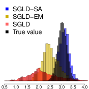
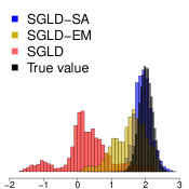
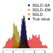
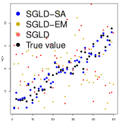
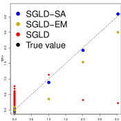
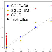
We conduct the linear regression experiments with a dataset containing $n=100$ observations and $p=1000$ predictors. $\mathcal{N}_{p}(0,\bm{\Sigma})$ is chosen to simulate the predictor values $\bm{X}$ (training set) where $\bm{\Sigma}=(\Sigma)_{i,j=1}^{p}$ with $\Sigma_{i,j}=0.6^{|i-j|}$. Response values $\bm{y}$ are generated from $\bm{X}\bm{\beta}+\bm{\eta}$, where $\bm{\beta}=(\beta_{1},\beta_{2},\beta_{3},0,0,...,0)^{\prime}$ and $\bm{\eta}\sim\mathcal{N}_{n}(\bm{0},3\bm{I}_{n})$. We assume $\beta_{1}\sim\mathcal{N}(3,\sigma_{c}^{2})$, $\beta_{2}\sim\mathcal{N}(2,\sigma_{c}^{2})$, $\beta_{3}\sim\mathcal{N}(1,\sigma_{c}^{2})$, $\sigma_{c}=0.2$. We introduce some hyperparameters, but most of them are uninformative. We fix $\tau=1,\lambda=1,\nu=1,v_{1}=10,\delta=0.5,b=p$ and set $a=1$. The learning rate follows $\epsilon^{(k)}=0.001\times k^{-\frac{1}{3}}$, and the step size is given by $\omega^{(k)}=10\times(k+1000)^{-0.7}$. We vary $v_{0}$ and $\sigma$ to show the robustness of SGLD-SA to different initializations. In addition, to show the superiority of the adaptive update, we compare SGLD-SA with the intuitive implementation of the EMVS to SGLD and refer to this algorithm as SGLD-EM, which is equivalent to setting $\omega^{(k)}:=1$ in SGLD-SA. To obtain the stochastic gradient, we randomly select 50 observations and calculate the numerical gradient. SGLD is sampled from the same hierarchical model without updating the latent variables.
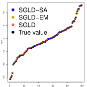
We simulate $500,000$ samples from the posterior distribution, and also simulate a test set with 50 observations to evaluate the prediction. As shown in Fig.1 (d), all three algorithms are fitted very well in the training set, however, SGLD fails completely in the test set (Fig.1 (e)), indicating the over-fitting problem of SGLD without proper regularization when the latent variables are not updated. Fig.1 (f) shows that although SGLD-EM successfully identifies the right variables, the estimations are lower biased. The reason is that SGLD-EM fails to regulate the right variables with $L_{2}$ penalty, and $L_{1}$ leads to a greater amount of shrinkage for $\bm{\beta}_{1}$, $\bm{\beta}_{2}$ and $\bm{\beta}_{3}$ (Fig. 1 (a-c)), implying the importance of the adaptive update via SA in the stochastic optimization of the latent variables. In addition, from Fig. 1(a), Fig. 1(b) and Fig.1(c), we see that SGLD-SA is the only algorithm among the three that quantifies the uncertainties of $\beta_{1}$, $\beta_{2}$ and $\beta_{3}$ and always gives the best prediction as shown in Table.1. We notice that SGLD-SA is fairly robust to various hyperparameters.

For the simulation of SGLD-SA in logistic regression and the evaluation of SGLD-SA on UCI datasets, we leave the results in Appendix C and D.

Table 1: Predictive errors in linear regression based on a test set considering different $v_{0}$ and $\sigma$
MAE / MSE $v_{0}$=$0.01,\sigma$=2 $v_{0}$=$0.1,\sigma$=2 $v_{0}$=$0.01,\sigma$=1 $v_{0}$=$0.1,\sigma$=1
SGLD-SA 1.89 / 5.56 1.72 / 5.64 1.48 / 3.51 1.54 /   4.42
SGLD-EM 3.49 / 19.31 2.23 / 8.22 2.23 / 19.28 2.07 /   6.94
SGLD 15.85 / 416.39 15.85 / 416.39 11.86 / 229.38 7.72 / 88.90
Refer to caption
(a) Posterior estimation of $\beta_{1}$.
Refer to caption
(b) Posterior estimation of $\beta_{2}$.
Refer to caption
(c) Posterior estimation of $\beta_{3}$.
Refer to caption
(d) Training performance.
Refer to caption
(e) Testing performance.
Refer to caption
(f) Posterior mean vs truth.
Figure 1: Linear regression simulation when $v_{0}=0.1$ and $\sigma=1$.

5.2 Classification with Auto-tuning Hyperparameters

The following experiments are based on non-pruning SG-MCMC-SA, the goal is to show that auto-tuning sparse priors are useful to avoid over-fitting. The posterior average is applied to each Bayesian model. We implement all the algorithms in Pytorch (Paszke et al., 2017). The first DNN is a standard 2-Conv-2-FC CNN model of 670K parameters (see details in Appendix D.1).

The first set of experiments is to compare methods on the same model without using data augmentation (DA) and batch normalization (BN) (Ioffe and Szegedy, 2015). We refer to the general CNN without dropout as Vanilla, with 50% dropout rate applied to the hidden units next to FC1 as Dropout.

Vanilla and Dropout models are trained with Adam (Kingma and Ba, 2014) and Pytorch default parameters (with learning rate 0.001). We use SGHMC as a benchmark method as it is also sampling-based and has a close relationship with the popular momentum based optimization approaches in DNNs. SGHMC-SA differs from SGHMC in that SGHMC-SA keeps updating SSGL priors for the first FC layer while they are fixed in SGHMC. We set the training batch size $n=1000$, $a,b=p$ and $\nu,\lambda=1000$. The hyperparameters for SGHMC-SA are set to $v_{0}=1,v_{1}=0.1$ and $\sigma=1$ to regularize the over-fitted space. The learning rate is set to $5\times 10^{-7}$, and the step size is $\omega^{(k)}=1\times(k+1000)^{-\frac{3}{4}}$. We use a thinning factor 500 to avoid a cumbersome system. Fixed temperature can also be powerful in escaping “shallow" local traps (Zhang et al., 2017), our temperatures are set to $\tau=1000$ for MNIST and $\tau=2500$ for FMNIST.

The four CNN models are tested on MNIST and Fashion MNIST (FMNIST) (Xiao et al., 2017) dataset. Performance of these models is shown in Tab.2. Compared with SGHMC, our SGHMC-SA outperforms SGHMC on both datasets. We notice the posterior averages from SGHMC-SA and SGHMC obtain much better performance than Vanilla and Dropout. Without using either DA or BN, SGHMC-SA achieves 99.59% which outperforms some state-of-the-art models, such as Maxout Network (99.55%) (Goodfellow et al., 2013) and pSGLD (99.55%) (Li et al., 2016) . In F-MNIST, SGHMC-SA obtains 93.01% accuracy, outperforming all other competing models.

To further test the performance, we apply DA and BN to the following experiments (see details in Appendix D.2) and refer to the datasets as DA-MNIST and DA-FMNIST. All the experiments are conducted using a 2-Conv-BN-3-FC CNN of 490K parameters. Using this model, we obtain the state-of-the-art 99.75% on DA-MNIST (200 epochs) and 94.38% on DA-FMNIST (1000 epochs) as shown in Tab. 2. The results are noticeable, because posterior average is only conducted on a single shallow CNN.

Table 2: Classification accuracy using shallow networks
Dataset MNIST DA-MNIST FMNIST DA-FMNIST
Vanilla 99.31 99.54 92.73 93.14
Dropout 99.38 99.56 92.81 93.35
SGHMC 99.47 99.63 92.88 94.29
SGHMC-SA 99.59 99.75 93.01 94.38

5.3 Defenses against Adversarial Attacks

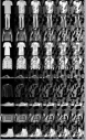
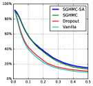
Continuing with the setup in Sec. 5.2, the third set of experiments focuses on evaluating model robustness. We apply the Fast Gradient Sign method (Goodfellow et al., 2014) to generate the adversarial examples with one single gradient step:

$$\bm{x}_{adv}\leftarrow\bm{x}-\zeta\cdot\operatorname{sign}\{\delta_{\bm{x}}\max_{\operatorname*{y}}\log\mathrm{P}(\operatorname*{y}|\bm{x})\},$$

where $\zeta$ ranges from $0.1,0.2,\ldots,0.5$ to control the different levels of adversarial attacks.

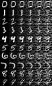
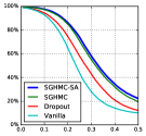
Similar to the setup in Li and Gal (2017), we normalize the adversarial images by clipping to the range $[0,1]$. In Fig. 2(b) and Fig.2(d), we see no significant difference among all the four models in the early phase. As the degree of adversarial attacks arises, the images become vaguer as shown in Fig.2(a) and Fig.2(c). The performance of Vanilla decreases rapidly, reflecting its poor defense against adversarial attacks, while Dropout performs better than Vanilla. But Dropout is still significantly worse than the sampling based methods. The advantage of SGHMC-SA over SGHMC becomes more significant when $\zeta>0.25$. In the case of $\zeta=0.5$ in MNIST where the images are hardly recognizable, both Vanilla and Dropout models fail to identify the right images and their predictions are as worse as random guesses. However, SGHMC-SA model achieves roughly 11% higher than these two models and 1% higher than SGHMC, which demonstrates the robustness of SGHMC-SA.

Refer to caption
(a) $\zeta=...$.
Refer to caption
(b) MNIST
Refer to caption
(c) $\zeta=...$.
Refer to caption
(d) FMNIST
Figure 2: Adversarial test accuracies based on adversarial images of different levels

5.4 Residual Network Compression

Our compression experiments are conducted on the CIFAR-10 dataset (Krizhevsky, 2009) with DA. SGHMC and the non-adaptive SGHMC-EM are chosen as baselines. Simulated annealing is used to enhance the non-convex optimization and the methods with simulated annealing are referred to as A-SGHMC, A-SGHMC-EM and A-SGHMC-SA, respectively. We report the best point estimate.

We first use SGHMC to train a Resnet20 model and apply the magnitude-based criterion to prune weights to all convolutional layers (except the very first one). All the following methods are evaluated based on the same setup except for different step sizes to learn the latent variables. The sparse training takes 1000 epochs. The mini-batch size is 1000. The learning rate starts from 2e-9 222It is equivalent to setting the learning rate to 1e-4 when we don’t multiply the likelihood with $\frac{N}{n}$. and is divided by 10 at the 700th and 900th epoch. We set the inverse temperature $\tau$ to 1000 and multiply $\tau$ by 1.005 every epoch . We fix $\nu=1000$ and $\lambda=1000$ for the inverse gamma prior. $v_{0}$ and $v_{1}$ are tuned based on different sparsity to maximize the performance. The smooth increase of the sparse rate follows the pruning rule in Algorithm 1, and $\mathbb{D}$ and $\mathbb{f}$ are set to $0.99$ and $50$, respectively. The increase in the sparse rate $s$ is faster in the beginning and slower in the later phase to avoid destroying the network structure. Weight decay in the non-sparse layers $\mathcal{C}$ is set as 25.

Table 3: Resnet20 Compression on CIFAR10. When $\mathbb{S}=0.9$, we fix $v_{0}=0.005$, $v_{1}=$1e-5; When $\mathbb{S}=0.7$, we fix $v_{0}=0.1$, $v_{1}=$5e-5; When $\mathbb{S}=0.5$, we fix $v_{0}=0.1$, $v_{1}=$5e-4; When $\mathbb{S}=0.3$, we fix $v_{0}=0.5$, $v_{1}=$1e-3.
Methods $\backslash$ $\ \mathbb{S}$ $30\%$ $50\%$ $70\%$ $90\%$
A-SGHMC 94.07 94.16 93.16 90.59
A-SGHMC-EM 94.18 94.19 93.41 91.26
SGHMC-SA 94.13 94.11 93.52 91.45
A-SGHMC-SA 94.23 94.27 93.74 91.68

As shown in Table 3, A-SGHMC-SA doesn’t distinguish itself from A-SGHMC-EM and A-SGHMC when the sparse rate $\mathbb{S}$ is small, but outperforms the baselines given a large sparse rate. The pretrained model has accuracy 93.90%, however,the prediction performance can be improved to the state-of-the-art $94.27\%$ with 50% sparsity. Most notably, we obtain 91.68% accuracy based on 27K parameters (90% sparsity) in Resnet20. By contrast, targeted dropout obtained 91.48% accuracy based on 47K parameters (90% sparsity) of Resnet32 (Gomez et al., 2018), BC-GHS achieves 91.0% accuracy based on 8M parameters (94.5% sparsity) of VGG models (Louizos et al., 2017). We also notice that when simulated annealing is not used as in SGHMC-SA, the performance will decrease by 0.2% to 0.3%. When we use batch size 2000 and inverse temperature schedule $\tau^{(k)}=20\times 1.01^{k}$, A-SGHMC-SA still achieves roughly the same level, but the prediction of SGHMC-SA can be 1% lower than A-SGHMC-SA.

6 Conclusion

We propose a novel AEB method to adaptively sample from hierarchical Bayesian DNNs and optimize the spike-and-slab priors, which yields a class of scalable adaptive sampling algorithms in DNNs. We prove the convergence of this approach to the asymptotically correct distribution. By adaptively searching and penalizing the over-fitted parameters, the proposed method achieves higher prediction accuracy over the traditional SG-MCMC methods in both simulated examples and real applications and shows more robustness towards adversarial attacks. Together with the magnitude-based weight pruning strategy and simulated annealing, the AEB-based method, A-SGHMC-SA, obtains the state-of-the-art performance in model compression.

Acknowledgments

We would like to thank Prof. Vinayak Rao, Dr. Yunfan Li and the reviewers for their insightful comments. We acknowledge the support from the National Science Foundation (DMS-1555072, DMS-1736364, DMS-1821233 and DMS-1818674) and the GPU grant program from NVIDIA.

References

  • Andrieu et al. (2005) Christophe Andrieu, Éric Moulines, and Pierre Priouret. Stability of Stochastic Approximation under Verifiable Conditions. SIAM J. Control Optim., 44(1):283–312, 2005.
  • Benveniste et al. (1990) Albert Benveniste, Michael Métivier, and Pierre Priouret. Adaptive Algorithms and Stochastic Approximations. Berlin: Springer, 1990.
  • Chen et al. (2015) Changyou Chen, Nan Ding, and Lawrence Carin. On the Convergence of Stochastic Gradient MCMC Algorithms with High-order Integrators. In Proc. of the Conference on Advances in Neural Information Processing Systems (NeurIPS), pages 2278–2286, 2015.
  • Chen et al. (2014) Tianqi Chen, Emily B. Fox, and Carlos Guestrin. Stochastic Gradient Hamiltonian Monte Carlo. In Proc. of the International Conference on Machine Learning (ICML), 2014.
  • Dalalyan and Karagulyan (2018) Arnak S. Dalalyan and Avetik G. Karagulyan. User-friendly Guarantees for the Langevin Monte Carlo with Inaccurate Gradient. ArXiv e-prints, September 2018.
  • George and McCulloch (1993) Edward I. George and Robert E. McCulloch. Variable Selection via Gibbs Sampling. Journal of the American Statistical Association, 88(423):881–889, 1993.
  • Ghosh et al. (2018) Soumya Ghosh, Jiayu Yao, and Finale Doshi-Velez. Structured Variational Learning of Bayesian Neural Networks with Horseshoe Priors. In Proc. of the International Conference on Machine Learning (ICML), 2018.
  • Gomez et al. (2018) Aidan N. Gomez, Ivan Zhang, Kevin Swersky, Yarin Gal, and Geoffrey E. Hinton. Targeted Dropout. In NeurIPS 2018 workshop on Compact Deep Neural Networks with industrial applications, 2018.
  • Goodfellow et al. (2013) Ian J. Goodfellow, David Warde-Farley, Mehdi Mirza, Aaron Courville, and Yoshua Bengio. Maxout networks. In Proc. of the International Conference on Machine Learning (ICML), pages III–1319–III–1327, 2013.
  • Goodfellow et al. (2014) Ian J. Goodfellow, Jonathon Shlens, and Christian Szegedy. Explaining and Harnessing Adversarial Examples. ArXiv e-prints, December 2014.
  • Han et al. (2016) Song Han, Huizi Mao, and William J Dally. Deep compression: Compressing Deep Neural Network with Pruning, Trained Quantization and Huffman Coding. In The IEEE Conference on Computer Vision and Pattern Recognition (CVPR), 2016.
  • He et al. (2016) Kaiming He, Xiangyu Zhang, Shaoqing Ren, and Jian Sun. Deep Residual Learning for Image Recognition. In The IEEE Conference on Computer Vision and Pattern Recognition (CVPR), 2016.
  • Hernandez-Lobato and Adams (2015) Jose Miguel Hernandez-Lobato and Ryan Adams. Probabilistic Backpropagation for Scalable Learning of Bayesian Neural Networks. In Proc. of the International Conference on Machine Learning (ICML), volume 37, pages 1861–1869, 2015.
  • Ioffe and Szegedy (2015) Sergey Ioffe and Christian Szegedy. Batch Normalization: Accelerating Deep Network Training by Reducing Internal Covariate Shift. In Proc. of the International Conference on Machine Learning (ICML), pages 448–456, 2015.
  • Jarrett et al. (2009) K. Jarrett, K. Kavukcuoglu, M. Ranzato, and Y. LeCun. What is the best multi-stage architecture for object recognition? In Proc. of the International Conference on Computer Vision (ICCV), pages 2146–2153, September 2009.
  • Kingma and Ba (2014) Diederik P. Kingma and Jimmy Ba. Adam: A Method for Stochastic Optimization. In Proc. of the International Conference on Learning Representation (ICLR), 2014.
  • Kirkpatrick et al. (1983) Scott Kirkpatrick, D. Gelatt Jr, and Mario P. Vecchi. Optimization by Simulated Annealing. Science, 220(4598):671–680, 1983.
  • Krizhevsky (2009) Alex Krizhevsky. Learning Multiple Layers of Features from Tiny Images. In Tech Report, 2009.
  • Li et al. (2016) Chunyuan Li, Changyou Chen, David Carlson, and Lawrence Carin. Preconditioned Stochastic Gradient Langevin Dynamics for Deep Neural Networks. In Proc. of the National Conference on Artificial Intelligence (AAAI), pages 1788–1794, 2016.
  • Li and Gal (2017) Yingzhen Li and Yarin Gal. Dropout Inference in Bayesian Neural Networks with Alpha-divergences. In Proc. of the International Conference on Machine Learning (ICML), 2017.
  • Liang (2010) Faming Liang. Trajectory Averaging for Stochastic Approximation MCMC Algorithms. The Annals of Statistics, 38:2823–2856, 2010.
  • Liang et al. (2018) Faming Liang, Bochao Jia, Jingnan Xue, Qizhai Li, and Ye Luo. Bayesian Neural Networks for Selection of Drug Sensitive Genes. Journal of the American Statistical Association, 113(5233):955–972, 2018.
  • Lin et al. (2017) Ji Lin, Yongming Rao, Jiwen Lu, and Jie Zhou. Runtime Neural Pruning. In Proc. of the Conference on Advances in Neural Information Processing Systems (NeurIPS), 2017.
  • Louizos et al. (2017) Christos Louizos, Karen Ullrich, and Max Welling. Bayesian Compression for Deep learning. In Proc. of the Conference on Advances in Neural Information Processing Systems (NeurIPS), 2017.
  • Ma et al. (2015) Yi-An Ma, Tianqi Chen, and Emily B. Fox. A Complete Recipe for Stochastic Gradient MCMC. In Proc. of the Conference on Advances in Neural Information Processing Systems (NeurIPS), 2015.
  • Mangoubi and Vishnoi (2018) Oren Mangoubi and Nisheeth K. Vishnoi. Convex Optimization with Unbounded Nonconvex Oracles using Simulated Annealing. In Proc. of Conference on Learning Theory (COLT), 2018.
  • Marinari and Parisi (1992) E Marinari and G Parisi. Simulated Tempering: A New Monte Carlo Scheme. Europhysics Letters (EPL), 19(6):451–458, 1992.
  • Mattingly et al. (2010) Jonathan C. Mattingly, Andrew M. Stuart, and M.V. Tretyakov. Convergence of Numerical Time-Averaging and Stationary Measures via Poisson Equations. SIAM Journal on Numerical Analysis, 48:552–577, 2010.
  • Molchanov et al. (2017) Pavlo Molchanov, Stephen Tyree, Tero Karras, Timo Aila, and Jan Kautz. Pruning Convolutional Neural Networks for Resource Efficient Inference. In Proc. of the International Conference on Learning Representation (ICLR), 2017.
  • Paszke et al. (2017) Adam Paszke, Sam Gross, Soumith Chintala, Gregory Chanan, Edward Yang, Zachary DeVito, Zeming Lin, Alban Desmaison, Luca Antiga, and Adam Lerer. Automatic differentiation in PyTorch. In NeurIPS Autodiff Workshop, 2017.
  • Raginsky et al. (2017) Maxim Raginsky, Alexander Rakhlin, and Matus Telgarsky. Non-convex Learning via Stochastic Gradient Langevin Dynamics: a Nonasymptotic Analysis. In Proc. of Conference on Learning Theory (COLT), June 2017.
  • Rořková and George (2014) Veronika Rořková and Edward I. George. EMVS: The EM Approach to Bayesian variable selection. Journal of the American Statistical Association, 109(506):828–846, 2014.
  • Rořková and George (2018) Veronika Rořková and Edward I. George. The Spike-and-Slab Lasso. Journal of the American Statistical Association, 113:431–444, 2018.
  • Saatci and Wilson (2017) Yunus Saatci and Andrew G Wilson. Bayesian GAN. In Proc. of the Conference on Advances in Neural Information Processing Systems (NeurIPS), pages 3622–3631, 2017.
  • Simonyan and Zisserman (2014) Karen Simonyan and Andrew Zisserman. Very Deep Convolutional Networks for Large-scale Image Recognition. In The IEEE Conference on Computer Vision and Pattern Recognition (CVPR), 2014.
  • Swendsen and Wang (1986) Robert H. Swendsen and Jian-Sheng Wang. Replica Monte Carlo Simulation of Spin-Glasses. Phys. Rev. Lett., 57:2607–2609, 1986.
  • Teh et al. (2016) Yee Whye Teh, Alexandre Thiéry, and Sebastian Vollmer. Consistency and Fluctuations for Stochastic Gradient Langevin Dynamics. Journal of Machine Learning Research, 17:1–33, 2016.
  • Tibshirani (1994) Robert Tibshirani. Regression Shrinkage and Selection via the Lasso. Journal of the Royal Statistical Society, Series B, 58:267–288, 1994.
  • Welling and Teh (2011) Max Welling and Yee Whye Teh. Bayesian Learning via Stochastic Gradient Langevin Dynamics. In Proc. of the International Conference on Machine Learning (ICML), pages 681–688, 2011.
  • Wong and Liang (1997) Wing Hung Wong and Faming Liang. Dynamic Weighting in Monte Carlo and Optimization. Proc. Natl. Acad. Sci., 94:14220–14224, 1997.
  • Xiao et al. (2017) Han Xiao, Kashif Rasul, and Roland Vollgraf. Fashion-MNIST: a Novel Image Dataset for Benchmarking Machine Learning Algorithms. ArXiv e-prints, August 2017.
  • Xu et al. (2018) Pan Xu, Jinghui Chen, Difan Zou, and Quanquan Gu. Global Convergence of Langevin Dynamics Based Algorithms for Nonconvex Optimization. In Proc. of the Conference on Advances in Neural Information Processing Systems (NeurIPS), December 2018.
  • Ye and Sun (2018) Mao Ye and Yan Sun. Variable Selection via Penalized Neural Network: a Drop-Out-One Loss Approach. In Proc. of the International Conference on Machine Learning (ICML), volume 80, pages 5620–5629, 10–15 Jul 2018.
  • Zhang et al. (2017) Yuchen Zhang, Percy Liang, and Moses Charikar. A Hitting Time Analysis of Stochastic Gradient Langevin Dynamics. In Proc. of Conference on Learning Theory (COLT), pages 1980–2022, 2017.
  • Zhong et al. (2020) Zhun Zhong, Liang Zheng, Guoliang Kang, Shaozi Li, and Yi Yang. Random Erasing Data Augmentation. In Proc. of the National Conference on Artificial Intelligence (AAAI), 2020.
  • Zou and Hastie (2005) Hui Zou and Trevor Hastie. Regularization and Variable Selection via the Elastic Net. Journal of the Royal Statistical Society, Series B, 67(2):301–320, 2005.

Supplimentary Material for An Adaptive Empirical Bayesian Method for Sparse Deep Learning

Wei Deng, Xiao Zhang, Faming Liang, Guang Lin

Purdue University, West Lafayette, IN, USA

{deng106, zhang923, fmliang, guanglin}@purdue.edu

In this supplementary material, we review the related methodologies in $\S$A, prove the convergence in $\S$B, present additional simulation of logistic regression in $\S$C, illustrate more regression examples on UCI datasets in $\S$D, and show the experimental setup in $\S$E.

Appendix A Stochastic Approximation

A.1 Special Case: Robbins–Monro Algorithm

Robbins–Monro algorithm is the first stochastic approximation algorithm to deal with the root finding problem which also applies to the stochastic optimization problem. Given the random output of $H(\bm{\theta},\bm{\beta})$ with respect to $\bm{\beta}$, our goal is to find the equilibrium $\bm{\theta}^{*}$ such that

$$\begin{split}h(\bm{\theta}^{*})&=\mathbb{E}[H(\bm{\theta}^{*},\bm{\beta})]=\int H(\bm{\theta}^{*},\bm{\beta})f_{\bm{\theta}*}(d\bm{\beta})=0,\end{split}$$ (16)

where $\mathbb{E}_{\bm{\theta}^{*}}$ denotes the expectation with respect to the distribution of $\bm{\beta}$ given $\bm{\theta}^{*}$. To implement the Robbins–Monro Algorithm, we can generate iterates as followsWe change the notation a little bit, where $\bm{\beta}_{k}\in\mathbb{R}^{d}$ and $\bm{\theta}_{k}$ are the parameters at the $k$-th iteration.:

  • (1)

    Sample $\bm{\beta}_{k+1}$ from the invariant distribution $f_{\bm{\theta}_{k}}(\bm{\beta})$,

  • (2)

    Update $\bm{\theta}_{k+1}=\bm{\theta}_{k}+\omega_{k+1}H(\bm{\theta}_{k},\bm{\beta}_{k+1}).$

Note that in this algorithm, $H(\bm{\theta},\bm{\beta})$ is the unbiased estimator of $h(\bm{\theta})$, that is for $k\in\mathrm{N}^{+}$, we have

$$\mathbb{E}_{\bm{\theta}_{k}}[H(\bm{\theta}_{k},\bm{\beta}_{k+1})-h(\bm{\theta}_{k})|\mathcal{F}_{k}]=0.$$ (17)

If there exists an antiderivative $Q(\bm{\theta},\bm{\beta})$ that satisfies $H(\bm{\theta},\bm{\beta})=\nabla_{\bm{\theta}}Q(\bm{\theta},\bm{\beta})$ and $E_{\bm{\theta}}[Q(\bm{\theta},\bm{\beta})]$ is concave, it is equivalent to solving the stochastic optimization problem $\max_{\bm{\theta}\in\bm{\Theta}}E_{\bm{\theta}}[Q(\bm{\theta},\bm{\beta})]$.

A.2 General Stochastic Approximation

The stochastic approximation algorithm is an iterative recursive algorithm consisting of two steps:

  • (1)

    Sample $\bm{\beta}_{k+1}$ from the transition kernel $\mathrm{\Pi}_{\bm{\theta_{k}}}(\bm{\beta}_{k},\cdot)$, which admits $f_{\bm{\theta}_{k}}(\bm{\beta})$ as the invariant distribution,

  • (2)

    Update $\bm{\theta}_{k+1}=\bm{\theta}_{k}+\omega_{k+1}H(\bm{\theta}_{k},\bm{\beta}_{k+1})$.

The general stochastic approximation [Benveniste et al., 1990] differs from the Robbins-Monro algorithm in that sampling $x$ from a transition kernel instead of a distribution introduces a Markov state-dependent noise $H(\theta_{k},x_{k+1})-h(\theta_{k})$.

Appendix B Convergence Analysis

B.1 Convergence of Hidden Variables

The stochastic gradient Langevin Dynamics with a stochastic approximation adaptation (SGLD-SA) is a mixed half-optimization-half-sampling algorithm to handle complex Bayesian posterior with latent variables, e.g. the conjugate spike-slab hierarchical prior formulation. Each iteration of the algorithm consists of the following steps:

  • (1)

    Sample $\bm{\beta}_{k+1}$ using SGLD based on $\bm{\theta}_{k}$, i.e.

    $$\begin{split}\bm{\beta}_{k+1}=\bm{\beta}_{k}+\epsilon\nabla_{\bm{\beta}}\tilde{L}(\bm{\beta}_{k},\bm{\theta}_{k})+\sqrt{{2\epsilon\tau^{-1}}}\bm{\eta}_{k},\end{split}$$ (18)

    where $\bm{\eta}_{k}\sim\mathcal{N}(0,\bm{I})$;

  • (2)

    Optimize $\bm{\theta}_{k+1}$ from the following recursion

$$\begin{split}\bm{\theta}_{k+1}&=\bm{\theta}_{k}+\omega_{k+1}\left(g_{\bm{\theta}_{k}}(\bm{\beta}_{k+1})-\bm{\theta}_{k}\right)\\ &=(1-\omega_{k+1})\bm{\theta}_{k}+\omega_{k+1}\bm{g}_{\bm{\theta}_{k}}(\bm{\beta}_{k+1}),\\ \end{split}$$ (19)

where $\bm{g}_{\bm{\theta}_{k}}(\cdot)$ is some mapping to derive the optimal $\bm{\theta}$ based on the current $\bm{\beta}$.

Remark: Define ${H(\bm{\theta}_{k},\bm{\beta}_{k+1})=g_{\bm{\theta}_{k}}(\bm{\beta}_{k+1})-\bm{\theta}_{k}}$. In this formulation, our target is to find $\bm{\theta}$ that solves $h(\bm{\theta})=\mathbb{E}[H(\bm{\theta},\bm{\beta})]=0$.

General Assumptions

To provide the $L_{2}$ upper bound for SGLD-SA, we first lay out the following assumptions:

Assumption 1 (Step size and Stability).

$\{\omega_{k}\}_{k\in\mathrm{N}}$ is a positive decreasing sequence of real numbers such that

$$\begin{split}&\omega_{k}\rightarrow 0,\ \ \sum_{k=1}^{\infty}\omega_{k}=+\infty.\end{split}$$ (20)

There exist $\delta>0$ and $\bm{\theta}^{*}$ such that for $\bm{\theta}\in\bm{\Theta}$: §§§$\|\cdot\|$ is short for $\|\cdot\|_{2}$

$$\begin{split}\langle\bm{\theta}-\bm{\theta}^{*},h(\bm{\theta})\rangle&\leq-\delta\|\bm{\theta}-\bm{\theta^{*}}\|^{2},\\ \end{split}$$ (21)

with additionally

$$\begin{split}\lim_{k\rightarrow\infty}\inf 2\delta\dfrac{\omega_{k}}{\omega_{k+1}}+\dfrac{\omega_{k+1}-\omega_{k}}{{\omega_{k+1}^{2}}}>0.\end{split}$$ (22)

Then for any $\alpha\in(0,1]$ and suitable $A$ and $B$, a practical $\omega_{k}$ can be set as

$$\begin{split}\omega_{k}=A(k+B)^{-\alpha}\end{split}$$ (23)
Assumption 2 (Smoothness).

$L(\bm{\beta},\bm{\theta})$ is $M$-smooth with $M>0$, i.e. for any $\bm{\beta},\bm{\iota}\in\bm{B}$, $\bm{\theta},\bm{\upsilon}\in\bm{\Theta}$.

$$\begin{split}&\|\nabla_{\bm{\beta}}L(\bm{\beta},\bm{\theta})-\nabla_{\bm{\beta}}L(\bm{\iota},\bm{\upsilon})\|\leq M\|\bm{\beta}-\bm{\iota}\|+M\|\bm{\theta}-\bm{\upsilon}\|.\end{split}$$ (24)
Assumption 3 (Dissipativity).

There exist constants $m>0,b\geq 0$, s.t. for all $\bm{\beta}\in\bm{\beta}$ and $\bm{\theta}\in\bm{\Theta}$, we have

$$\langle\nabla_{\bm{\beta}}L(\bm{\beta},\bm{\theta}),\bm{\beta}\rangle\leq b-m\|\bm{\beta}\|^{2}.$$ (25)
Assumption 4 (Gradient condition).

The stochastic noise $\bm{\chi}_{k}\in\bm{B}$, which comes from $\nabla_{\bm{\beta}}\tilde{L}(\bm{\beta}_{k},\bm{\theta}_{k})-\nabla_{\bm{\beta}}L(\bm{\beta}_{k},\bm{\theta}_{k})$, is a white noise or Martingale difference noise and is independent with each other.

$$\begin{split}\mathbb{E}[\bm{\chi}_{k}|\mathcal{\bm{F}}_{k}]&=0.\\ \end{split}$$ (26)

The scale of the noise is bounded by

$$\begin{split}\mathbb{E}\|\bm{\chi}\|^{2}\leq M^{2}\mathbb{E}\|\bm{\beta}\|^{2}+M^{2}\mathbb{E}\|\bm{\theta}\|^{2}+B^{2}.\\ \end{split}$$ (27)

for constants $M,B>0$.

In addition to the assumptions, we also assume the existence of Markov transition kernel, the proof goes beyond the scope of our paper.

Proposition 1.

There exist constants $M,B>0$ such that

$$\begin{split}\|g_{\bm{\theta}}(\bm{\beta})\|^{2}\leq M^{2}\|\bm{\beta}\|^{2}+B^{2}\end{split}$$ (28)
Proof.

As shown in Eq.(12), Eq.(13) and Eq.(15) in the main body, $\bm{\rho},\delta$ and $\bm{\kappa}$ are clearly bounded. It is also easy to verify that $\sigma$ in Eq.(14) in the main body satisfies (28). For convenience, we choose the same $M$ and $B$ (large enough) as in (27). ∎

Proposition 2.

For any $\bm{\beta}\in\bm{B}$, it holds that

$$\begin{split}\|\nabla_{\bm{\beta}}L(\bm{\beta},\bm{\theta})\|^{2}\leq 3M^{2}\|\bm{\beta}\|^{2}+3M^{2}\|\bm{\theta}\|^{2}+3B^{2}\end{split}$$ (29)

for constants $M$ and $B$.

Proof.

Suppose there is a minimizer $(\bm{\theta}^{*},\bm{\beta}^{*})$ such that $\nabla_{\bm{\beta}}L(\bm{\beta}^{*},\bm{\theta}^{*})=0$ and $\bm{\theta}^{*}$ has reached the stationary point, following Assumption 3 we have,

$$\begin{split}\langle\nabla_{\bm{\beta}}L(\bm{\beta}^{*},\bm{\theta}^{*}),\bm{\beta}^{*}\rangle\leq b-m\|\bm{\beta}^{*}\|^{2}.\\ \end{split}$$

Therefore, $\|\bm{\beta}^{*}\|^{2}\leq\frac{b}{m}$. Since $\bm{\theta}^{*}$ is the stationary point, $\bm{\theta}^{*}=(1-\omega)\bm{\theta}^{*}+\omega g_{\bm{\theta}^{*}}(\bm{\beta}^{*})$. By (28), we have $\|g_{\bm{\theta}^{*}}(\bm{\beta}^{*})\|^{2}\leq M^{2}\|\bm{\beta}^{*}\|^{2}+B^{2}$, which implies that $\|\bm{\theta}^{*}\|^{2}=\|g_{\bm{\theta}^{*}}(\bm{\beta}^{*})\|^{2}\leq M^{2}\|\bm{\beta}^{*}\|^{2}+B^{2}\leq\frac{b}{m}M^{2}+B^{2}$. By the smoothness assumption 2, we have

$$\begin{split}&\|\nabla_{\bm{\beta}}L(\bm{\beta},\bm{\theta})\|\\ \leq&\|\nabla_{\bm{\beta}}L(\bm{\beta}^{*},\bm{\theta}^{*})\|+M\|\bm{\beta}-\bm{\beta}^{*}\|+M\|\bm{\theta}-\bm{\theta}^{*}\|\\ \leq&0+M(\|\bm{\beta}\|+\sqrt{\frac{b}{m}}+\|\bm{\theta}\|+\|\bm{\theta}^{*}\|)\\ \leq&M\|\bm{\theta}\|+M\|\bm{\beta}\|+M(\sqrt{\frac{b}{m}}+\sqrt{\frac{b}{m}M^{2}+B^{2}})\\ \leq&M\|\bm{\theta}\|+M\|\bm{\beta}\|+\bar{B},\\ \end{split}$$

where $\bar{B}=M(\sqrt{\frac{b}{m}M^{2}+B^{2}}+\sqrt{\frac{b}{m}})$. Therefore,

$$\|\nabla_{\bm{\beta}}L(\bm{\beta},\bm{\theta})\|^{2}\leq 3M^{2}\|\bm{\beta}\|^{2}+3M^{2}\|\bm{\theta}\|^{2}+3\bar{B}^{2}.$$

For notation simplicity, we can choose the same $B$ (large enough) to bound (27), (28) and (29). ∎

Lemma 1 (Uniform $L_{2}$ bound).

For all $\ 0<\epsilon<\operatorname{Re}(\tfrac{m-\sqrt{m^{2}-4M^{2}(M^{2}+1)}}{4M^{2}(M^{2}+1)})$, there exist $G,\overline{G}>0$ such that $\sup\mathbb{E}\|\bm{\beta}_{k}\|^{2}\leq G$ and $\sup\mathbb{E}\|\bm{\theta}_{k}\|^{2}\leq\overline{G}$, where $G=\|\bm{\beta}_{0}\|^{2}+\tfrac{1}{m}(b+2\epsilon B^{2}(M^{2}+1)+\tau d)$ and $\overline{G}=M^{2}G+B^{2}$.

Proof.

From (18), we have

$$\begin{split}&\mathbb{E}\|\bm{\beta}_{k+1}\|^{2}\\ =&\mathbb{E}\left\|\bm{\beta}_{k}+\epsilon\nabla_{\bm{\beta}}\tilde{L}(\bm{\beta}_{k},\bm{\theta}_{k})\right\|^{2}+2\tau\epsilon\mathbb{E}\|\bm{\eta}_{k}\|^{2}+\sqrt{8\epsilon\tau}\mathbb{E}\langle\bm{\beta}_{k}+\epsilon\nabla_{\bm{\beta}}\tilde{L}(\bm{\beta}_{k},\bm{\theta}_{k}),\bm{\eta}_{k}\rangle\\ =&\mathbb{E}\left\|\bm{\beta}_{k}+\epsilon\nabla_{\bm{\beta}}\tilde{L}(\bm{\beta}_{k},\bm{\theta}_{k})\right\|^{2}+2\tau\epsilon d,\\ \end{split}$$ (30)

Moreover, the first item in (LABEL:eq:21) can be expanded to

$$\begin{split}&\ \ \ \mathbb{E}\left\|\bm{\beta}_{k}+\epsilon\nabla_{\bm{\beta}}\tilde{L}(\bm{\beta}_{k},\bm{\theta}_{k})\right\|^{2}\\ &=\mathbb{E}\left\|\bm{\beta}_{k}+\epsilon\nabla_{\bm{\beta}}L(\bm{\beta}_{k},\bm{\theta}_{k})\right\|^{2}+\epsilon^{2}\mathbb{E}\left\|\bm{\chi}_{k}\right\|^{2}-2\epsilon\mathbb{E}\left[\mathbb{E}\left(\langle\bm{\beta}_{k}+\epsilon\nabla_{\bm{\beta}}L(\bm{\beta}_{k},\bm{\theta}_{k}),\bm{\chi}_{k}\rangle|\mathcal{F}_{k}\right)\right]\\ &=\mathbb{E}\left\|\bm{\beta}_{k}+\epsilon\nabla_{\bm{\beta}}L(\bm{\beta}_{k},\bm{\theta}_{k})\right\|^{2}+\epsilon^{2}\mathbb{E}\left\|\bm{\chi}_{k}\right\|^{2},\end{split}$$ (31)

where (26) is used to cancel the inner product item.

Turning to the first item of (LABEL:eq:22), the dissipivatity condition (25) and the boundness of $\nabla_{\bm{\beta}}L(\bm{\beta},\bm{\theta})$ (29) give us:

$$\begin{split}&\ \ \ \ \ \mathbb{E}\left\|\bm{\beta}_{k}+\epsilon\nabla_{\bm{\beta}}L(\bm{\beta}_{k},\bm{\theta}_{k})\right\|^{2}\\ &=\mathbb{E}\|\bm{\beta}_{k}\|^{2}+2\epsilon\mathbb{E}\langle\bm{\beta}_{k},\nabla_{\bm{\beta}}L(\bm{\beta}_{k},\bm{\theta}_{k})\rangle+\epsilon^{2}\mathbb{E}\left\|\nabla_{\bm{\beta}}L(\bm{\beta}_{k},\bm{\theta}_{k})\right\|^{2}\\ &\leq\mathbb{E}\|\bm{\beta}_{k}\|^{2}+2\epsilon(b-m\mathbb{E}\|\bm{\beta}_{k}\|^{2})+\epsilon^{2}(3M^{2}\mathbb{E}\|\bm{\beta}_{k}\|^{2}+3M^{2}\mathbb{E}\|\bm{\theta}_{k}\|^{2}+3B^{2})\\ &=(1-2\epsilon m+3\epsilon^{2}M^{2})\mathbb{E}\|\bm{\beta}_{k}\|^{2}+2\epsilon b+3\epsilon^{2}B^{2}+3\epsilon^{2}M^{2}\mathbb{E}\|\bm{\theta}_{k}\|^{2}.\end{split}$$ (32)

By (27), the second item of (LABEL:eq:22) is bounded by

$$\begin{split}\mathbb{E}\|\bm{\chi}_{k}\|^{2}\leq M^{2}\mathbb{E}\|\bm{\beta}_{k}\|^{2}+M^{2}\mathbb{E}\|\bm{\theta}_{k}\|^{2}+B^{2}.\\ \end{split}$$ (33)

Combining (LABEL:eq:21), (LABEL:eq:22), (LABEL:eq:27) and (33), we have

$$\begin{split}&\mathbb{E}\|\bm{\beta}_{k+1}\|^{2}\leq(1-2\epsilon m+4\epsilon^{2}M^{2})\mathbb{E}\|\bm{\beta}_{k}\|^{2}+2\epsilon b+4\epsilon^{2}B^{2}+4\epsilon^{2}M^{2}\mathbb{E}\|\bm{\theta}_{k}\|^{2}+2\tau\epsilon d.\\ \end{split}$$ (34)

Next we use proof by induction to show for $k=1,2,\ldots,\infty$, $\mathbb{E}\|\bm{\beta}_{k}\|^{2}\leq G$, where

$$G=\mathbb{E}\|\bm{\beta}_{0}\|^{2}+\dfrac{b+2\epsilon B^{2}(M^{2}+1)+\tau d}{m-2\epsilon M^{2}(M^{2}+1)}.$$ (35)

First of all, the case of $k=0,1$ is trivial. Then if we assume for each $k\in 2,3,\ldots,t$, $\mathbb{E}\|\bm{\beta}_{k}\|^{2}\leq G$, $\mathbb{E}\|g(\bm{\beta}_{k})\|^{2}\leq M^{2}G+B^{2}$, $\mathbb{E}\|\bm{\theta}_{k-1}\|^{2}\leq M^{2}G+B^{2}$. It follows that,

$$\begin{split}&\ \ \ \ \ \mathbb{E}\|\bm{\theta}_{k}\|^{2}=\mathbb{E}\|(1-\omega_{k})\bm{\theta}_{k-1}+\omega_{k}g(\bm{\beta}_{k})\|^{2}\\ &\leq(1-\omega_{k})^{2}\mathbb{E}\|\bm{\theta}_{k-1}\|^{2}+{\omega_{k}}^{2}\mathbb{E}\|g(\bm{\beta}_{k})\|^{2}+2(1-\omega_{k})\omega_{k}\mathbb{E}\langle\bm{\theta}_{k-1},g(\bm{\beta}_{k})\rangle\\ &\leq(1-\omega_{k})^{2}\mathbb{E}\|\bm{\theta}_{k-1}\|^{2}+{\omega_{k}}^{2}\mathbb{E}\|g(\bm{\beta}_{k})\|^{2}+2(1-\omega_{k})\omega_{k}\sqrt{\mathbb{E}\|\bm{\theta}_{k-1}\|^{2}\mathbb{E}\|g(\bm{\beta}_{k})\|^{2}}\\ &\leq(1-\omega_{k})^{2}(M^{2}G+B^{2})+{\omega_{k}}^{2}(M^{2}G+B^{2})+2(1-\omega_{k})\omega_{k}(M^{2}G+B^{2})\\ &=M^{2}G+B^{2},\end{split}$$

Next, we proceed to prove $\mathbb{E}\|\bm{\beta}_{t+1}\|^{2}\leq G$ and $\mathbb{E}\|\bm{\theta}_{t+1}\|^{2}\leq M^{2}G+B^{2}$. Following (LABEL:eq:29), we have

$$\begin{split}&\ \ \ \ \ \mathbb{E}\|\bm{\beta}_{t+1}\|^{2}\\ &\leq(1-2\epsilon m+4\epsilon^{2}M^{2})\mathbb{E}\|\bm{\beta}_{k}\|^{2}+2\epsilon b+4\epsilon^{2}B+4\epsilon^{2}M^{2}\mathbb{E}\|\bm{\theta}_{k}\|^{2}+2\tau\epsilon d\\ &\leq(1-2\epsilon m+4\epsilon^{2}M^{2})G+2\epsilon b+4\epsilon^{2}B+4\epsilon^{2}M^{2}(M^{2}G+B^{2})+2\tau\epsilon d\\ &\leq\left(1-2\epsilon m+4\epsilon^{2}M^{2}(M^{2}+1)\right)G+2\epsilon b+4\epsilon^{2}B^{2}(M^{2}+1)+2\tau\epsilon d\\ \end{split}$$ (36)

Consider the quadratic equation $1-2mx+4M^{2}(M^{2}+1)x^{2}=0$. If $m^{2}-4M^{2}(M^{2}+1)\geq 0$, then the smaller root is $\tfrac{m-\sqrt{m^{2}-4M^{2}(M^{2}+1)}}{4M^{2}(M^{2}+1)}$ which is positive; otherwise the quadratic equation has no real solutions and is always positive. Fix $\epsilon\in\left(0,\operatorname{Re}\left(\tfrac{m-\sqrt{m^{2}-4M^{2}(M^{2}+1)}}{4M^{2}(M^{2}+1)}\right)\right)$ so that

$$0<1-2\epsilon m+4\epsilon^{2}M^{2}(M^{2}+1)<1.$$ (37)

With (35), we can further bound (LABEL:eq:30) as follows:

$$\begin{split}&\ \ \ \ \ \mathbb{E}\|\bm{\beta}_{t+1}\|^{2}\\ &\leq\left(1-2\epsilon m+4\epsilon^{2}M^{2}(M^{2}+1)\right)\left(\mathbb{E}\|\bm{\beta}_{0}\|^{2}+\mathbb{I}\right)+2\epsilon b+4\epsilon^{2}B^{2}(M^{2}+1)+2d\tau\epsilon\\ &=\left(1-2\epsilon m+4\epsilon^{2}M^{2}(M^{2}+1)\right)\mathbb{E}\|\bm{\beta}_{0}\|^{2}+\mathbb{I}-\left(2\epsilon b+4\epsilon^{2}B^{2}(M^{2}+1)+2d\tau\epsilon\right)\\ &\ \ \ +\left(2\epsilon b+4\epsilon^{2}B^{2}(M^{2}+1)+2\epsilon\tau d\right)\\ &\leq\mathbb{E}\|\bm{\beta}_{0}\|^{2}+\mathbb{I}\equiv G,\end{split}$$ (38)

where $\mathbb{I}=\dfrac{b+2\epsilon B^{2}(M^{2}+1)+d\tau}{m-2\epsilon M^{2}(M^{2}+1)}$, the second to the last inequality comes from (37).

Moreover, from (28), we also have

$$\begin{split}\mathbb{E}\|g(\bm{\beta}_{t+1})\|^{2}&\leq M^{2}\mathbb{E}\|\bm{\beta}_{t+1}\|^{2}+B^{2}\leq M^{2}G+B^{2},\\ \end{split}$$
$$\begin{split}&\ \ \ \mathbb{E}\|\bm{\theta}_{t+1}\|^{2}=\mathbb{E}\|(1-\omega_{t+1})\bm{\theta}_{t}+\omega_{t+1}g(\bm{\beta}_{t+1})\|^{2}\\ &\leq(1-\omega_{t+1})^{2}\mathbb{E}\|\bm{\theta}_{t}\|^{2}+\omega_{t+1}^{2}\mathbb{E}\|g(\bm{\beta}_{t+1})\|^{2}+2(1-\omega_{t+1})\omega_{t+1}\mathbb{E}\langle\bm{\theta}_{t},g(\bm{\beta}_{t+1})\rangle\\ &\leq(1-\omega_{t+1})^{2}\mathbb{E}\|\bm{\theta}_{t}\|^{2}+\omega_{t+1}^{2}\mathbb{E}\|g(\bm{\beta}_{t+1})\|^{2}+2(1-\omega_{t+1})\omega_{t+1}\sqrt{\mathbb{E}\|\bm{\theta}_{t}\|^{2}\mathbb{E}\|g(\bm{\beta}_{t+1})\|^{2}}\\ &\leq(1-\omega_{t+1})^{2}(M^{2}G+B^{2})+\omega_{t+1}^{2}(M^{2}G+B^{2})+2(1-\omega_{t+1})\omega_{t+1}(M^{2}G+B^{2})\\ &=M^{2}G+B^{2},\end{split}$$

Therefore, we have proved that for any $k\in 1,2,\ldots,\infty$, $\mathbb{E}\|\bm{\beta}_{k}\|^{2}$, $\mathbb{E}\|g(\bm{\beta}_{k})\|^{2}$ and $\mathbb{E}\|\bm{\theta}_{k}\|^{2}$ are bounded. Furthermore, we notice that $G$ can be unified to a constant $G=\mathbb{E}\|\bm{\beta}_{0}\|^{2}+\tfrac{1}{m}\left(b+2\epsilon B^{2}(M^{2}+1)+\tau d\right)$. ∎

Assumption 5 (Solution of Poisson equation).

For all $\bm{\theta}\in\bm{\Theta}$, $\bm{\beta}\in\bm{B}$ and a function $V(\bm{\beta})=1+\|\bm{\beta}\|^{2}$, there exists a function $\mu_{\bm{\theta}}(\cdot)$ on $\bm{B}$ that solves the Poisson equation $\mu_{\bm{\theta}}(\bm{\beta})-\mathrm{\Pi}_{\bm{\theta}}\mu_{\bm{\theta}}(\bm{\beta})=H(\bm{\theta},\bm{\beta})-h(\bm{\theta})$, which follows that

$$\begin{split}&H(\bm{\theta}_{k},\bm{\beta}_{k+1})=h(\bm{\theta}_{k})+\mu_{\bm{\theta}_{k}}(\bm{\beta}_{k+1})-\mathrm{\Pi}_{\bm{\theta}_{k}}\mu_{\bm{\theta}_{k}}(\bm{\beta}_{k+1}).\end{split}$$ (39)

Moreover, for all $\bm{\theta},\bm{\theta}^{\prime}\in\bm{\Theta}$ and $\bm{\beta}\in\bm{B}$, we have

$$\begin{split}\|\mu_{\bm{\theta}}(\bm{\beta})-\mu_{\bm{\theta^{\prime}}}(\bm{\beta})\|&\lesssim\|\bm{\theta}-\bm{\theta}^{\prime}\|V(\bm{\beta}),\\ \|\mu_{\bm{\theta}}(\bm{\beta})\|&\lesssim V(\bm{\beta})\end{split}$$

Poisson equation has been widely in controlling the perturbations of adaptive algorithms [Benveniste et al., 1990, Andrieu et al., 2005, Liang, 2010]. Following Benveniste et al. [1990], we only impose the 1st-order smoothness on the solution of Poisson equation, which is much weaker than the 4th-order smoothness used in proving the ergodicity theory [Mattingly et al., 2010, Teh et al., 2016]. The verification of the above assumption is left as future works.

Proposition 3.

The uniform $L_{2}$ bound in lemma 1 further implies that $\mathbb{E}[V(\bm{\beta})]<\infty$. In what follows, there exists a constant $C$ such that

$$\begin{split}\mathbb{E}[\|\mathrm{\Pi}_{\bm{\theta}}\mu_{\bm{\theta}}(\bm{\beta})-\mathrm{\Pi}_{\bm{\theta}^{\prime}}\mu_{\bm{\theta^{\prime}}}(\bm{\beta})\|]&\leq C\|\bm{\theta}-\bm{\theta}^{\prime}\|,\\ \mathbb{E}[\|\mathrm{\Pi}_{\bm{\theta}}\mu_{\bm{\theta}}(\bm{\beta})\|]&\leq C.\end{split}$$ (40)
Proposition 4.

There exists a constant $C_{1}$ so that

$$\begin{split}&\mathbb{E}[\|H(\bm{\theta},\bm{\beta})\|^{2}]\leq C_{1}(1+\|\bm{\theta}-\bm{\theta}^{*}\|^{2})\\ \end{split}$$ (41)
Proof.

By (28), we have

$$\begin{split}\mathbb{E}\|g_{\bm{\theta}}(\bm{\beta})-\bm{\theta}\|^{2}&\leq 2\mathbb{E}\|g_{\bm{\theta}}(\bm{\beta})\|^{2}+2\|\bm{\theta}\|^{2}\leq 2(M^{2}\mathbb{E}\|\bm{\beta}\|^{2}+B^{2})+2\|\bm{\theta}\|^{2}\\ \end{split}$$

Given the boundness of $\mathbb{E}\|\bm{\beta}\|^{2}$ and a large enough $C^{\prime}=\max(2,2(M^{2}\mathbb{E}\|\bm{\beta}\|^{2}+B^{2}))$, we have

$$\begin{split}&\mathbb{E}[\|H(\bm{\theta},\bm{\beta})\|^{2}]\leq C^{\prime}(1+\|\bm{\theta}\|^{2})=C^{\prime}(1+\|\bm{\theta}-\bm{\theta}^{*}+\bm{\theta}^{*}\|^{2})\leq C_{1}(1+\|\bm{\theta}-\bm{\theta}^{*}\|^{2})\\ \end{split}$$

Lemma 2 is a restatement of Lemma 25 (page 247) from Benveniste et al. [1990].

Lemma 2.

Suppose $k_{0}$ is an integer which satisfies with

$$\begin{split}\inf_{k\geq k_{0}}\dfrac{\omega_{k+1}-\omega_{k}}{\omega_{k}\omega_{k+1}}+2\delta-\omega_{k+1}C_{1}>0.\end{split}$$

Then for any $k>k_{0}$, the sequence $\{\Lambda_{k}^{K}\}_{k=k_{0},\ldots,K}$ defined below is increasing

$$\left\{\begin{array}[]{lr}2\omega_{k}\prod_{j=k}^{K-1}(1-2\omega_{j+1}\delta+\omega_{j+1}^{2}C_{1})&\text{if $k<K$},\\ &\\ 2\omega_{k}&\text{if $k=K$}.\end{array}\right.$$ (42)

This following lemma is proved by Benveniste et al. [1990] and we present it here for reader’s convenience.

Lemma 3.

There exist $\lambda_{0}$ and $k_{0}$ such that for all $\lambda\geq\lambda_{0}$ and $k\geq k_{0}$, the sequence $u_{k}=\lambda\omega_{k}$ satisfies

$$\begin{split}u_{k+1}\geq&(1-2\omega_{k+1}\delta+{\omega_{k+1}^{2}}C_{1})u_{k}+{\omega_{k+1}^{2}}\overline{C}_{1}.\end{split}$$ (43)
Proof.

By replacing $u_{k}=\lambda\omega_{k}$ in (43), we need to prove the following

$$\begin{split}\lambda\omega_{k+1}\geq&(1-2\omega_{k+1}\delta+{\omega_{k+1}^{2}}C_{1})\lambda\omega_{k}+{\omega_{k+1}^{2}}\overline{C}_{1}.\end{split}$$ (44)

According to (22) in assumption 1, there exists a positive constant $C_{+}$ such that

$$\omega_{k+1}-\omega_{k}+2\omega_{k}\omega_{k+1}\geq C_{+}\omega_{k+1}^{2},$$ (45)

Combining (44) and (45), it suffices to show

$$\begin{split}\lambda(C_{+}-\omega_{k}C_{1})\geq\overline{C}_{1}.\end{split}$$ (46)

Apparently, there exist $\lambda_{0}$ and $k_{0}$ such that for all $\lambda>\lambda_{0}$ and $k>k_{0}$, (46) holds. ∎

Theorem 1 ($L_{2}$ convergence rate). Suppose that Assumptions 1-5 hold, there exists a constant $\lambda$ such that

$$\begin{split}\mathbb{E}\left[\|\bm{\theta}_{k}-\bm{\theta}^{*}\|^{2}\right]\leq\lambda\omega_{k},\end{split}$$
Proof.

Denote $\bm{T}_{k}=\bm{\theta}_{k}-\bm{\theta}^{*}$, with the help of (19) and Poisson equation (LABEL:a4.ii), we deduce that

$$\begin{split}&\|\bm{T}_{k+1}\|^{2}\\ =&\|\bm{T}_{k}\|^{2}+{\omega_{k+1}^{2}}\|H(\bm{\theta}_{k},\bm{\beta}_{k+1})\|^{2}+2\omega_{k+1}\langle\bm{T}_{k},H(\bm{\theta}_{k},\bm{\beta}_{k+1})\rangle\\ =&\|\bm{T}_{k}\|^{2}+{\omega_{k+1}^{2}}\|H(\bm{\theta}_{k},\bm{\beta}_{k+1})\|^{2}+2\omega_{k+1}\langle\bm{T}_{k},h(\bm{\theta}_{k})\rangle+2\omega_{k+1}\langle\bm{T}_{k},\mu_{\bm{\theta}_{k}}(\bm{\beta}_{k+1})-\mathrm{\Pi}_{\bm{\theta}_{k}}\mu_{\bm{\theta}_{k}}(\bm{\beta}_{k+1})\rangle\\ =&\|\bm{T}_{k}\|^{2}+\text{D1}+\text{D2}+\text{D3}.\\ \end{split}$$

First of all, according to (LABEL:bound2) and (21), we have

$\displaystyle{\omega_{k+1}^{2}}\mathbb{E}[\|H(\bm{\theta}_{k},\bm{\beta}_{k+1})\|^{2}]$ $\displaystyle\leq{\omega_{k+1}^{2}}C_{1}(1+\|\bm{T}_{k}\|^{2}),$ (D1)
$\displaystyle 2\omega_{k+1}\mathbb{E}[\langle\bm{T}_{k},h(\bm{\theta}_{k})\rangle]$ $\displaystyle\leq-2\omega_{k+1}\delta\|\bm{T}_{k}\|^{2},$ (D2)

Conduct the decomposition of D3 similar to Theorem 24 (p.g. 246) from Benveniste et al. [1990] and Lemma A.5 [Liang, 2010].

$$\begin{split}&\mu_{\bm{\theta}_{k}}(\bm{\beta}_{k+1})-\mathrm{\Pi}_{\bm{\theta}_{k}}\mu_{\bm{\theta}_{k}}(\bm{\beta}_{k+1})\\ =&\underbrace{\mu_{\bm{\theta}_{k}}(\bm{\beta}_{k+1})-\mathrm{\Pi}_{\bm{\theta}_{k}}\mu_{\bm{\theta}_{k}}(\bm{\beta}_{k})}_{\text{D3-1}}+\underbrace{\mathrm{\Pi}_{\bm{\theta}_{k}}\mu_{\bm{\theta}_{k}}(\bm{\beta}_{k})-\mathrm{\Pi}_{\bm{\theta}_{k-1}}\mu_{\bm{\theta}_{k-1}}(\bm{\beta}_{k})}_{\text{D3-2}}+\underbrace{\mathrm{\Pi}_{\bm{\theta}_{k-1}}\mu_{\bm{\theta}_{k-1}}(\bm{\beta}_{k})-\mathrm{\Pi}_{\bm{\theta}_{k}}\mu_{\bm{\theta}_{k}}(\bm{\beta}_{k+1})}_{\text{D3-3}}.\\ \end{split}$$

(i) $\mu_{\bm{\theta}_{k}}(\bm{\beta}_{k+1})-\mathrm{\Pi}_{\bm{\theta}_{k}}\mu_{\bm{\theta}_{k}}(\bm{\beta}_{k})$ forms a martingale difference sequence such that

$$\mathbb{E}\left[\mu_{\bm{\theta}_{k}}(\bm{\beta}_{k+1})-\mathrm{\Pi}_{\bm{\theta}_{k}}\mu_{\bm{\theta}_{k}}(\bm{\beta}_{k})|\mathcal{F}_{k}\right]=0.$$ (D3-1)D3-1

(ii) From Lemma 1, we have that $\mathbb{E}[\|\bm{T_{k}}\|]$ is bounded. In addition, following Cauchy–Schwarz inequality and the regularity conditions in (40), there exists a positive constant $C_{2}$ such that

$\displaystyle\mathbb{E}\left[2\omega_{k+1}\langle\bm{T}_{k},\mathrm{\Pi}_{\bm{\theta}_{k}}\mu_{\bm{\theta}_{k}}(\bm{\beta}_{k})-\mathrm{\Pi}_{\bm{\theta}_{k-1}}\mu_{\bm{\theta}_{k-1}}(\bm{\beta}_{k})\rangle\right]\leq\omega_{k+1}^{2}C_{2}.$ (D3-2)

(iii) D3-3 can be further decomposed to D3-3a and D3-3b

$$\small\begin{split}&\ \ \ \langle\bm{T}_{k},\mathrm{\Pi}_{\bm{\theta}_{k-1}}\mu_{\bm{\theta}_{k-1}}(\bm{\beta}_{k})-\mathrm{\Pi}_{\bm{\theta}_{k}}\mu_{\bm{\theta}_{k}}(\bm{\beta}_{k+1})\rangle\\ &=\left(\langle\bm{T}_{k},\mathrm{\Pi}_{\bm{\theta}_{k-1}}\mu_{\bm{\theta}_{k-1}}(\bm{\beta}_{k})\rangle-\langle\bm{T}_{k+1},\mathrm{\Pi}_{\bm{\theta}_{k}}\mu_{\bm{\theta}_{k}}(\bm{\beta}_{k+1})\rangle\right)+\left(\langle\bm{T}_{k+1},\mathrm{\Pi}_{\bm{\theta}_{k}}\mu_{\bm{\theta}_{k}}(\bm{\beta}_{k+1})\rangle-\langle\bm{T}_{k},\mathrm{\Pi}_{\bm{\theta}_{k}}\mu_{\bm{\theta}_{k}}(\bm{\beta}_{k+1})\rangle\right)\\ &=\underbrace{(z_{k}-z_{k+1})}_{\text{D3-3a}}+\underbrace{\langle\bm{T}_{k+1}-\bm{T}_{k},\mathrm{\Pi}_{\bm{\theta}_{k}}\mu_{\bm{\theta}_{k}}(\bm{\beta}_{k+1})\rangle}_{\text{D3-3b}}.\\ \end{split}$$

where $z_{k}=\langle\bm{T}_{k},\mathrm{\Pi}_{\bm{\theta}_{k-1}}\mu_{\bm{\theta}_{k-1}}(\bm{\beta}_{k})\rangle$. Combining (19), (28), Lemma 1 and Cauchy–Schwarz inequality, there exists a constant $C_{3}$ such that

$\displaystyle\mathbb{E}\left[2\omega_{k+1}\langle\bm{T}_{k+1}-\bm{T}_{k},\mathrm{\Pi}_{\bm{\theta}_{k}}\mu_{\bm{\theta}_{k}}(\bm{\beta}_{k+1})\rangle\right]\leq\omega_{k+1}^{2}C_{3}$

Finally, add all the items D1, D2 and D3 together, for some $\overline{C}_{1}=C_{1}+C_{2}+C_{3}$, we have

$$\begin{split}&\mathbb{E}\left[\|\bm{T}_{k+1}\|^{2}\right]\leq(1-2\omega_{k+1}\delta+{\omega_{k+1}^{2}}C_{1})\mathbb{E}\left[\|\bm{T}_{k}\|^{2}\right]+{\omega_{k+1}^{2}}\overline{C}_{1}+2\omega_{k+1}\mathbb{E}[z_{k}-z_{k+1}].\end{split}$$

Moreover, from (40), there exists a constant $C_{4}$ such that

$$\begin{split}\mathbb{E}[|z_{k}|]\leq C_{4}.\end{split}$$ (47)

Lemma 4 is a restatement of Lemma 26 (page 248) from Benveniste et al. [1990].

Lemma 4.

Let $\{u_{k}\}_{k\geq k_{0}}$ as a sequence of real numbers such that for all $k\geq k_{0}$, some suitable constants $\overline{C}_{1}$ and $C_{1}$

$$\begin{split}u_{k+1}\geq&u_{k}\left(1-2\omega_{k+1}\delta+{\omega_{k+1}^{2}}C_{1}\right)+{\omega_{k+1}^{2}}\overline{C}_{1},\end{split}$$ (48)

and assume there exists such $k_{0}$ that

$$\begin{split}\mathbb{E}\left[\|\bm{T}_{k_{0}}\|^{2}\right]\leq u_{k_{0}}.\end{split}$$ (49)

Then for all $k>k_{0}$, we have

$$\begin{split}\mathbb{E}\left[\|\bm{T}_{k}\|^{2}\right]\leq u_{k}+\sum_{j=k_{0}+1}^{k}\Lambda_{j}^{k}(z_{j-1}-z_{j}).\end{split}$$

Proof of Theorem 1 (Continued). From Lemma 3, we can choose $\lambda_{0}$ and $k_{0}$ which satisfy the conditions (48) and (49)

$\displaystyle\mathbb{E}[\|\bm{T}_{k_{0}}\|^{2}]\leq u_{k_{0}}=\lambda_{0}\omega_{k_{0}}.$

From Lemma 4, it follows that for all $k>k_{0}$

$$\begin{split}\mathbb{E}\left[\|\bm{T}_{k}\|^{2}\right]\leq u_{k}+\mathbb{E}\left[\sum_{j=k_{0}+1}^{k}\Lambda_{j}^{k}\left(z_{j-1}-z_{j}\right)\right].\end{split}$$ (50)

From (47) and the increasing property of $\Lambda_{j}^{k}$ in Lemma 2, we have

$$\begin{split}&\mathbb{E}\left[\left|\sum_{j=k_{0}+1}^{k}\Lambda_{j}^{k}\left(z_{j-1}-z_{j}\right)\right|\right]\\ =&\mathbb{E}\left[\left|\sum_{j=k_{0}+1}^{k-1}(\Lambda_{j+1}^{k}-\Lambda_{j}^{k})z_{j}-2\omega_{k}z_{k}+\Lambda_{k_{0}+1}^{k}z_{k_{0}}\right|\right]\\ \leq&\sum_{j=k_{0}+1}^{k-1}(\Lambda_{j+1}^{k}-\Lambda_{j}^{k})C_{4}+\mathbb{E}[|2\omega_{k}z_{k}|]+\Lambda_{k}^{k}C_{4}\\ \leq&(\Lambda_{k}^{k}-\Lambda_{k_{0}}^{k})C_{4}+\Lambda_{k}^{k}C_{4}+\Lambda_{k}^{k}C_{4}\\ \leq&3\Lambda_{k}^{k}C_{4}=6C_{4}\omega_{k}.\end{split}$$ (51)

Therefore, given the sequence $u_{k}=\lambda_{0}\omega_{k}$ that satisfies conditions (48), (49) and Lemma 4, for any $k>k_{0}$, from (50) and (LABEL:eqn:10), we have

$$\mathbb{E}[\|\bm{T}_{k}\|^{2}]\leq u_{k}+3C_{4}\Lambda_{k}^{k}=\left(\lambda_{0}+6C_{4}\right)\omega_{k}=\lambda\omega_{k},$$

where $\lambda=\lambda_{0}+6C_{4}$. ∎

B.2 Weak Convergence of Samples

In statistical models with latent variables, the gradient is often biased due to the use of stochastic approximation. Langevin Monte Carlo with inaccurate gradients has been studied by Chen et al. [2015], Dalalyan and Karagulyan [2018], which are helpful to prove the weak convergence of samples. Following theorem 2 in Chen et al. [2015], we have

Corollary 1. Under assumptions in Appendix B.1 and the assumption 1 (smoothness and boundness on the solution functional) in Chen et al. [2015], the distribution of $\bm{\beta}_{k}$ converges weakly to the target posterior as $\epsilon\rightarrow 0$ and $k\rightarrow\infty$.

Proof.

Since $\bm{\theta}_{k}$ converges to $\bm{\theta}^{*}$ in SGLD-SA under assumptions in Appendix B.1 and the gradient is M-smooth (LABEL:ass_2_1_eq), we decompose the stochastic gradient $\nabla_{\bm{\beta}}\tilde{L}(\bm{\beta}_{k},\bm{\theta}_{k})$ as $\nabla_{\bm{\beta}}L(\bm{\beta}_{k},\bm{\theta}^{*})+\bm{\xi}_{k}+\mathcal{O}(k^{-\alpha})$, where $\nabla_{\bm{\beta}}L(\bm{\beta}_{k},\bm{\theta}^{*})$ is the exact gradient, $\bm{\xi}_{k}$ is a zero-mean random vector, $\mathcal{O}(k^{-\alpha})$ is the bias term coming from the stochastic approximation and $\alpha\in(0,1]$ is used to guarantee the consistency in theorem 1. Therefore, Eq.(18) can be written as

$$\begin{split}\bm{\beta}_{k+1}&=\bm{\beta}_{k}+\epsilon_{k}\left(\nabla_{\bm{\beta}}L(\bm{\beta}_{k},\bm{\theta}^{*})+\bm{\xi}_{k}+\mathcal{O}(k^{-\alpha})\right)+\sqrt{2\epsilon_{k}}\bm{\eta}_{k},\ \operatorname*{where}\ \bm{\eta}_{k}\sim\mathcal{N}(0,\bm{I}).\\ \end{split}$$ (52)

Following a similar proof in Chen et al. [2015], it suffices to show that $\sum_{k=1}^{K}k^{-\alpha}/K\rightarrow 0$ as $K\rightarrow\infty$, which is obvious. Therefore, the distribution of $\bm{\beta}_{k}$ converges weakly to the target distribution as $\epsilon\rightarrow 0$ and $k\rightarrow\infty$. ∎

Appendix C Simulation of Large-p-Small-n Logistic Regression

Now we conduct the experiments on binary logistic regression. The setup is similar as before, except $n$ is set to 500, $\Sigma_{i,j}=0.3^{|i-j|}$ and $\bm{\eta}\sim\mathcal{N}(0,\bm{I}/2)$. We set the learning rate for all the three algorithms to $0.001\times k^{-\frac{1}{3}}$ and step size $\omega_{k}$ to $10\times(k+1000)^{-0.7}$. The binary response values are simulated from $\textbf{Bernoulli}(p)$ where $p=1/(1+e^{-X\bm{\beta}-\bm{\eta}})$. As shown in Fig.3: SGLD fails in selecting the right variables and overfits the data; both SGLD-EM and SGLD-SA choose the right variables. However, SGLD-EM converges to a poor local optimum by mistakenly using $L_{1}$ norm to regularize all the variables, leading to a large shrinkage effect on $\bm{\beta}_{1:3}$. By contrast, SGLD-SA successfully updates the latent variables and regularize $\beta_{1:3}$ with $L_{2}$ norm, yielding a better parameter estimation for $\beta_{1:3}$ and a stronger regularization for $\beta_{4-1000}$. Table.4 illustrates that SGLD-SA consistently outperforms the other methods and is robust to different initializations. We observe that SGLD-EM sometimes performs as worse as SGLD when $v_{0}=0.001$, which indicates that the EM-based variable selection is not robust in the stochastic optimization of the latent variables.

Table 4: Predictive errors in logistic regression based on a test set considering different $v_{0}$ and $\sigma$
MAE / MSE $v_{0}$=$0.01,\sigma$=1 $v_{0}$=$0.001,\sigma$=1 $v_{0}$=$0.01,\sigma$=2 $v_{0}$=$0.001,\sigma$=2
SGLD-SA 0.177 / 0.108 0.188 / 0.114 0.182 / 0.116 0.187 / 0.113
SGLD-EM 0.207 / 0.131 0.361 / 0.346 0.204 / 0.132 0.376 / 0.360
SGLD 0.295 / 0.272 0.335 / 0.301 0.350 / 0.338 0.337 / 0.319
Refer to caption
Figure 3: Logistic regression simulation when $v_{0}=0.1$ and $\sigma=1$

Appendix D Regression on UCI datasets

We further evaluate our model on five UCI regression datasets and show the results in Table 5. Following Hernandez-Lobato and Adams [2015], we randomly sample 90% of each dataset for training and leave the rest for testing. We run 20 experiments for each setup with fixed random seeds and report the averaged error rate. Feature normalization is applied in the experiments. The model is a simple MLP with one hidden layer of 50 units. We set the batch size to 50, the training epoch to 200, the learning rate to 1e-5 and the default $L_{2}$ to 1e-4. For SGHMC-EM and SGHMC-SA, we apply the SSGL prior on the BNN weights (excluding biases) and fix $a,\nu,\lambda=1$, $b,v_{1},\sigma=10$ and $\delta=0.5$. We fine-tune the initial temperature $\tau$ and $v_{0}$. As shown in Table 5, SGHMC-SA outperforms all the baselines. Nevertheless, without smooth adaptive update, SGHMC-EM often performs worse than SGHMC. While with simulated annealing where $\tau^{(k)}=\tau\times 1.003^{k}$, we observe further improved performance in most of the cases.

Dataset Boston Yacht Energy Wine Concrete
Hyperparameters 1/0.1 1/0.1 0.1/0.1 0.5/0.01 0.5/0.07
SGHMC 2.783$\pm$0.109 0.886$\pm$0.046 1.983$\pm$0.092 0.731$\pm$0.015 6.319$\pm$0.179
A-SGHMC 2.848$\pm$0.126 0.808$\pm$0.048 1.419$\pm$0.067 0.671$\pm$0.019 5.978$\pm$0.166
SGHMC-EM 2.813$\pm$0.140 0.823$\pm$0.053 $2.077\pm$0.108 0.729$\pm$0.018 6.275$\pm$0.169
A-SGHMC-EM 2.767$\pm$0.154 0.815$\pm$0.052 1.435$\pm$0.069 0.627$\pm$0.008 5.762$\pm$0.156
SGHMC-SA 2.779$\pm$0.133 0.789$\pm$0.050 1.948$\pm$0.081 0.654$\pm$0.010 6.029$\pm$0.131
A-SGHMC-SA 2.692$\pm$0.120 0.782$\pm$0.052 1.388$\pm$0.052 0.620$\pm$0.008 5.687$\pm$0.142
Table 5: Average performance and standard deviation of Root Mean Square Error, where $\tau$ denotes the initial inverse temperature and $v_{0}$ is a hyperparameter in the SSGL prior (Hyperparameters $\tau/v_{0}$).

Appendix E Experimental Setup

E.1 Network Architecture

The first DNN we use is a standard 2-Conv-2-FC CNN: it has two convolutional layers with a 2 $\times$ 2 max pooling after each layer and two fully-connected layers. The filter size in the convolutional layers is 5 $\times$ 5 and the feature maps are set to be 32 and 64, respectively [Jarrett et al., 2009]. The fully-connected layers (FC) have 200 hidden nodes and 10 outputs. We use the rectified linear unit (ReLU) as activation function between layers and employ a cross-entropy loss.

The second DNN is a 2-Conv-BN-3-FC CNN: it has two convolutional layers with a $2\times 2$ max pooling after each layer and three fully-connected layers with batch normalization applied to the first FC layer. The filter size in the convolutional layers is $4\times 4$ and the feature maps are both set to 64. We use $256\times 64\times 10$ fully-connected layers.

E.2 Data Augmentation

The MNIST dataset is augmented by (1) randomCrop: randomly crop each image with size 28 and padding 4, (2) random rotation: randomly rotate each image by a degree in $[-15^{\circ},+15^{\circ}]$, (3) normalization: normalize each image with empirical mean 0.1307 and standard deviation 0.3081.

The FMNIST dataset is augmented by (1) randomCrop: same as MNIST, (2) randomHorizontalFlip: randomly flip each image horizontally, (3) normalization: same as MNIST, (4) random erasing [Zhong et al., 2020].

The CIFAR10 dataset is augmented by (1) randomCrop: randomly crop each image with size 32 and padding 4, (2) randomHorizontalFlip: randomly flip each image horizontally, (3) normalization: normalize each image with empirical mean (0.4914, 0.4822, 0.4465) and standard deviation (0.2023, 0.1994, 0.2010), (4) random erasing.