Abstract

We address the problem of computing reliable policies in reinforcement learning problems with limited data. In particular, we compute policies that achieve good returns with high confidence when deployed. This objective, known as the percentile criterion, can be optimized using Robust MDPs (RMDPs). RMDPs generalize MDPs to allow for uncertain transition probabilities chosen adversarially from given ambiguity sets. We show that the RMDP solution’s sub-optimality depends on the spans of the ambiguity sets along the value function. We then propose new algorithms that minimize the span of ambiguity sets defined by weighted $L_{1}$ and $L_{\infty}$ norms. Our primary focus is on Bayesian guarantees, but we also describe how our methods apply to frequentist guarantees and derive new concentration inequalities for weighted $L_{1}$ and $L_{\infty}$ norms. Experimental results indicate that our optimized ambiguity sets improve significantly on prior construction methods.

1 Introduction

Applying reinforcement learning to problem domains that involve high-stakes decisions, such as medicine or robotics, demands that we have high confidence in the quality of a policy before deploying it. Markov Decision Processes (MDPs) represent a well-established model in reinforcement learning (Puterman,, 2005; Sutton and Barto,, 2018), but their sequential nature makes them particularly sensitive to parameter errors, which can quickly accumulate (Mannor et al.,, 2007; Xu and Mannor,, 2009; Tirinzoni et al.,, 2018). Parameter errors are unavoidable when estimating MDPs from data Laroche et al., (2019). We focus on computing policies that maximize high-confidence return guarantees in the batch settings. Such guarantees reduce the chance of disappointing the stakeholders after deploying the policy and give them a choice to gather more data or switch to an alternative strategy Petrik et al., (2016).

We propose a new method for computing reliable policies that achieve, with high confidence, good returns once deployed. This objective is also known as the percentile criterion Delage and Mannor, (2010) and can be modeled as risk-aversion to epistemic uncertainty Petrik and Russel, (2019). Because optimizing the percentile criterion is NP-hard Delage and Mannor, (2010), we use Robust MDPs (RMDPs) Iyengar, (2005) to optimize it approximately. We establish new error bounds on the performance loss of the RMDPs’ policy compared to the optimal percentile solution. Using these new bounds when constructing the RMDPs leads to policies with significantly better return guarantees than reported in prior work Delage and Mannor, (2010); Petrik and Russel, (2019).

RMDPs generalize MDPs to allow for uncertain, or unknown, transition probabilities (Nilim and Ghaoui,, 2005; Iyengar,, 2005; Wiesemann et al.,, 2013). Transition probabilities are hard to estimate from data, and even small errors significantly impact the returns and policies. RMDPs consider transition probabilities to be chosen adversarially from a so-called ambiguity set (or an uncertainty set). The optimal policy is computed by solving a specific zero-sum game in which the agent chooses the best policy, and an adversarial nature chooses the worst transition probabilities from the ambiguity sets. RMDPs are tractable when their ambiguity sets satisfy so-called rectangularity assumptions Wiesemann et al., (2013); Mannor et al., (2016); Goyal and Grand-Clement, (2018).

Given the goal is to optimize the percentile criterion, the critical question is how to construct the ambiguity sets from state transition samples to optimize the percentile criterion. Prior work constructs ambiguity sets as confidence regions bounded by a distance from a nominal (expected) transition probability (Petrik et al.,, 2016; Petrik and Russel,, 2019; Auer et al.,, 2009; Strehl and Littman,, 2004; Gupta,, 2019; Iyengar,, 2005). In most cases, the ambiguity sets are represented as $L_{1}$-norm (also referred to as total variation) balls around the nominal probability. In comparison with other probability distance measures, like KL-divergence, the polyhedral nature of the $L_{1}$-norm allows more efficient computation Ho et al., (2018).

The main contribution of this paper is a new technique for optimizing the shape of ambiguity sets in RMDPs. Prior work simply constructs ambiguity sets with the smallest size, or volume, that is sufficient to provide the desired high-confidence guarantees. Our new bounds show that the span of the ambiguity set along a specific direction is much more important than its volume. To minimize their span, we consider asymmetric ambiguity sets defined in terms of weighted $L_{1}$ and $L_{\infty}$ balls. Recent results shows that RMDPs with such ambiguity sets can be solved very efficiently (Ho et al.,, 2018, 2020). Although our primary focus is on the Bayesian setup, we also discuss the frequentist setup and derive new high-confidence concentration inequalities for the weighted $L_{1}$ and $L_{\infty}$ norms.

The remainder of the paper is organized as follows. We first describe the necessary background in Section 2 and bound the performance loss of RMDPs as a function of the ambiguity sets’ span in Section 3. Section 4 describes algorithms that minimize the span of ambiguity sets by optimizing the weights of the norms used in their definition. Then, Section 5 describes methods for choosing the size of the weighted-norm ambiguity sets. In Section 6, we outline the approach in the frequentist setup and present new concentration inequalities for weighted $L_{1}$ and $\,L_{\infty}$ ambiguity sets. Finally, the experimental results in Section 7 show that minimizing ambiguity sets’ span greatly improves the RMDPs’ solution quality.

Notation: Bold letters, like ${\boldsymbol{x}}_{s}$, indicate an $s$-th vector, while $y_{s}$ would indicate the $s$-th element of a vector ${\boldsymbol{y}}$. The symbol $\Delta^{N}$ denotes the $N$-dimensional probability simplex (non-negative vectors that sum to $1$). We also use $\mathcal{A}^{\mathcal{B}}$ to denote the set of all functions $\mathcal{A}\to\mathcal{B}$.

2 Framework and Related Work

We consider the standard infinite-horizon MDP setting with finite states $\mathcal{S}=\{1,\ldots,S\}$ and actions $\mathcal{A}=\{1,\ldots,A\}$. The agent can take any action $a\in\mathcal{A}$ in every state $s\in\mathcal{S}$ and transitions to the next state $s^{\prime}$ according to the true transition function $P^{\star}:\mathcal{S}\times\mathcal{A}\to\Delta^{S}$, where $\Delta^{S}$ is a probability simplex. For any transition function $P:\mathcal{S}\times\mathcal{A}\to\Delta^{S}$, we use the shorthand ${\boldsymbol{p}}_{s,a}=P(s,a)$ to denote the vector of transition probabilities from a state $s\in\mathcal{S}$ and an action $a\in\mathcal{A}$. The agent also receives a reward $r_{s,a,s^{\prime}}\in\mathbb{R}$; we use ${\boldsymbol{r}}_{s,a}=(r_{s,a,s^{\prime}})_{s^{\prime}\in\mathcal{S}}\in\mathbb{R}^{S}$ to denote the vector of rewards. The goal is to compute a deterministic policy $\pi:\mathcal{S}\rightarrow\mathcal{A}$ that maximizes the $\gamma$-discounted return (Puterman,, 2005):

$$\max_{\pi\in\Pi}\;\rho(\pi,P)=\max_{\pi\in\Pi}\;\mathbb{E}\left[\sum_{t=0}^{\infty}\gamma^{t}\cdot r_{S_{t},\pi(S_{t}),S_{t+1}}\right]~{},$$

where $S_{0}\sim{\boldsymbol{p}}_{0}$, $S_{t+1}\sim P^{\star}(S_{t},\pi(S_{t}))$, ${\boldsymbol{p}}_{0}\in\Delta^{S}$ is the initial probability distribution, and $\Pi$ is the set of all deterministic policies. The return function $\rho$ is parameterized by $P$, because we assume them to be uncertain or unknown.

We consider the batch RL setting in which the transition function must be estimated from a fixed dataset $D=\left(s_{t},a_{t},s_{t}^{\prime}\right)_{t=1,\ldots,T}$ generated by a behavior policy. We describe the Bayesian setup first and outline the frequentist extension in Section 6. Bayesian techniques start with a prior distribution over the transition function $P^{\star}$ and then derive a posterior distribution $f$ over $P^{\star}$ (Delage and Mannor,, 2010; Xu and Mannor,, 2009; Gelman et al.,, 2014). We use the concise notation $\tilde{P}=P^{\star}\,|\,D$ to represent the posterior over the transition function conditioned on the data $D$. In other words, $\mathbb{E}[\tilde{P}]=\mathbb{E}[P^{\star}\,|\,D]$.

Percentile citerion

The Bayesian percentile criterion optimization simultaneously optimizes for the policy $\pi$ and a high-confidence lower bound on its performance $y$:

$$\max_{\pi\in\Pi}\max_{y\in\mathbb{R}}\;\left\{y\;|\;\mathbb{P}_{\tilde{P}\sim f}\left[\rho(\pi,\tilde{P})\geq y\right]\geq 1-\delta\right\}~{}.$$ (1)

The confidence parameter $\delta\in[0,\nicefrac{{1}}{{2}})$ bounds the probability that the optimized policy $\pi$ fails to achieve a return of at least $y$ when deployed. For example, $\delta=0$ maximizes the worst-case return, and $\delta=0.5$ maximizes the median return. It is common in practice to choose a small positive value, such as $\delta=0.05$, in order to achieve meaningful guarantees without being overly conservative. Also, the constraint $\delta<\nicefrac{{1}}{{2}}$ is important as our results (Theorem 3.2) do not hold for the risk-seeking setting with $\delta\geq\nicefrac{{1}}{{2}}$.

There are several important practical advantages to optimizing the percentile criterion instead of the average return Delage and Mannor, (2010). First, the output policy is more robust and less likely to fail catastrophically due to model errors. Second, the objective value $y$ in (1) provides a high-confidence lower bound on the true return. Having such a guarantee on its return helps to avoid an unpleasant surprise when the policy $\pi$ is deployed. If the guarantee $y$ is insufficiently low, the stakeholder may decide to collect more data or choose a different methodology for guiding their decisions.

We emphasize that we develop algorithms that are independent of how the posterior distribution $f$ is computed. Bayesian priors can be as simple as independent Dirichlet distributions over ${\boldsymbol{p}}^{\star}_{s,a}$ for each state $s$ and action $a$. However, hierarchical Bayesian models are more practical since they can generalize among states even when $|D|\ll S$ (Delage and Mannor,, 2010; Petrik and Russel,, 2019). Many tools, such as Stan Stan Development Team, (2017) or JAGS, now exist that allow for convenient and efficient computation of the posterior distribution $f$ using MCMC.

Robust MDPs

Because the optimization in (1) is NP-hard Delage and Mannor, (2010), we seek new algorithms that can approximate it efficiently. Robust MDPs (RMDPs), which extend regular MDPs, are a convenient and powerful framework that can be used to optimize the percentile criterion. In particular, RMDPs allow for a generic ambiguity set $\hat{\mathcal{P}}\subseteq\left\{P:\mathcal{S}\times\mathcal{A}\to\Delta^{S}\right\}$ of possible transition functions instead of a single known value $P$. The solution to an RMDP is the best policy for the worst-case plausible transition function:

$$\max_{\pi\in\Pi}\min_{P\in\hat{\mathcal{P}}}\,\rho(\pi,P)~{}.$$ (2)

The optimization problem in (2) is NP-hard (Nilim and Ghaoui,, 2005; Wiesemann et al.,, 2013) but is tractable for rectangular ambiguity sets which are defined independently for each state and action (Iyengar,, 2005; Le Tallec,, 2007). We, therefore, restrict our attention to SA-rectangular ambiguity sets defined as $p$-norm balls around nominal probability distributions for some $w:\mathcal{S}\times\mathcal{A}\to\mathbb{R}_{++}^{S}$ and $\psi:\mathcal{S}\times\mathcal{A}\to\mathbb{R}_{+}$:

$$\mathcal{P}(w,\psi)=\left\{P\in\mathcal{F}\;|\;P(s,a)\in\mathcal{P}_{s,a}(w(s,a),\psi(s,a))\right\},$$

where $\mathcal{F}=(\Delta^{S})^{\mathcal{S}\times\mathcal{A}}$. In the remainder of the paper, we resort to the shorter notation ${\boldsymbol{w}}_{s,a}=w(s,a)$ and $\psi_{s,a}=\psi(s,a)$ when the meaning is obvious from the context. Note that $\hat{\mathcal{P}}$ refers to a generic ambiguity set, while $\mathcal{P}(w,\psi)$ refers to the specific norm-based one. The ambiguity set $\mathcal{P}_{s,a}({\boldsymbol{w}},\psi)$ for $s\in\mathcal{S}$, $a\in\mathcal{A}$, positive weights ${\boldsymbol{w}}\in^{S}_{++}$, and budget $\psi\in\mathbb{R}_{+}$ is defined as:

$$\mathcal{P}_{s,a}({\boldsymbol{w}},\psi)=\left\{{\boldsymbol{p}}\in\Delta^{S}~{}:~{}\left\lVert{\boldsymbol{p}}-\bar{{\boldsymbol{p}}}_{s,a}\right\rVert_{{\boldsymbol{w}}}\leq\psi\right\},$$ (3)

where $\bar{{\boldsymbol{p}}}_{s,a}=\mathbb{E}_{\tilde{P}}\bigl{[}\tilde{P}(s,a)\bigr{]}$ is the mean posterior transition probability. The weighted polynomial norms are defined as $\left\lVert{\boldsymbol{y}}\right\rVert_{1,{\boldsymbol{w}}}=\sum_{i=1}^{S}w_{i}\cdot\lvert y_{i}\rvert$ and $\left\lVert{\boldsymbol{y}}\right\rVert_{\infty,{\boldsymbol{w}}}=\max\,\{w_{i}\cdot\lvert y_{i}\rvert\;|\;i\in\mathcal{S}\}$. We use the generic notation $\left\lVert\cdot\right\rVert_{{\boldsymbol{w}}}$ in statements that hold for both $\left\lVert\cdot\right\rVert_{1,{\boldsymbol{w}}}$ and $\left\lVert\cdot\right\rVert_{\infty,{\boldsymbol{w}}}$. The weights ${\boldsymbol{w}}$ in (3) determine the shape of the ambiguity set, and the budget $\psi$ determines its size.

Note that the parameter $\psi$ in the definition of $\mathcal{P}_{s,a}({\boldsymbol{w}},\psi)$ is redundant. It can be set to $1$ without loss of generality: $\mathcal{P}_{s,a}({\boldsymbol{w}},\psi)=\mathcal{P}_{s,a}(\nicefrac{{1}}{{\psi}}\cdot{\boldsymbol{w}},1)$ when $\psi>0$. In other words, it is possible to change the size of the ambiguity set solely by scaling the weights ${\boldsymbol{w}}$. To eliminate this redundancy, we assume without loss of generality that the weights of the set are normalized such that $\left\lVert{\boldsymbol{w}}\right\rVert_{2}=1$.

In rectangular RMDPs, a unique optimal value function $\hat{{\boldsymbol{v}}}\in\mathbb{R}^{S}$ exists and is a fixed point of the robust Bellman operator $\mathfrak{L}:\mathbb{R}^{S}\to\mathbb{R}^{S}$ defined for each $s\in\mathcal{S}$ and ${\boldsymbol{v}}\in\mathbb{R}^{S}$ as Iyengar, (2005)

$$(\mathfrak{L}\,{\boldsymbol{v}})_{s}=\max_{a\in\mathcal{A}}\min_{{\boldsymbol{p}}\in\hat{\mathcal{P}}_{s,a}}\,\Bigl{(}{\boldsymbol{r}}_{s,a}+\gamma\cdot{\boldsymbol{p}}^{\mkern-1.5mu\mathsf{T}}{\boldsymbol{v}}\Bigr{)}~{}.$$ (4)

The optimal robust value function can be computed using value iteration, policy iteration, and other methods Iyengar, (2005); Kaufman and Schaefer, (2013); Ho et al., (2020). The optimal robust policy $\hat{\pi}:\mathcal{S}\to\mathcal{A}$ is greedy with respect to the optimal robust value function $\hat{{\boldsymbol{v}}}$, and the robust return can be computed from the value function as Ho et al., (2020):

$$\hat{\rho}\;=\;\max_{\pi\in\Pi}\min_{P\in\hat{\mathcal{P}}}\;\rho(\pi,P)\;=\;{\boldsymbol{p}}_{0}^{\mkern-1.5mu\mathsf{T}}\hat{{\boldsymbol{v}}}~{}.$$

We will find it convenient to use $\hat{{\boldsymbol{z}}}_{s,a}\in\mathbb{R}^{S},\,s\in\mathcal{S},a\in\mathcal{A}$ to denote the vector of values associated with the transitions from the state $s$ and action $a$:

$$\hat{{\boldsymbol{z}}}_{s,a}\;=\;{\boldsymbol{r}}_{s,a}+\gamma\cdot\hat{{\boldsymbol{v}}}~{}.$$ (5)

In the remainder of the paper, we use $\hat{\mathcal{P}}$ to denote a generic RMDP ambiguity set and use $\mathcal{P}(w,\psi)$ to denote an ambiguity set defined in terms of a weighted norm ball.

3 RMDPs for Percentile Optimization

This section describes the general algorithm for constructing RMDP ambiguity sets for optimizing the percentile criterion. We derive new bounds on the safety and optimality of the RMDP solution and propose a new algorithm that optimizes them. The bounds and algorithms in this section are general and are not restricted to norm-based ambiguity sets.

An important assumption, which is used throughout this paper, is that the ambiguity set in the RMDP is constructed to guarantee that it contains the unknown transition probabilities $\tilde{P}$ with a high probability as formalized next.

Assumption 1.

The RMDP ambiguity set $\hat{\mathcal{P}}\subseteq\left\{P:\mathcal{S}\times\mathcal{A}\to\Delta^{S}\right\}$ satisfies that:

$$\mathbb{P}_{\tilde{P}}\bigl{[}\tilde{P}\in\hat{\mathcal{P}}\bigr{]}\;\geq\;1-\delta\,.$$

1 is common when constructing RMDPs for optimizing the percentile criterion Petrik and Russel, (2019); Delage and Mannor, (2010). The following theorem shows that 1 is a sufficient condition for $\hat{\rho}$ to be a lower bound on the true return of the robust policy $\hat{\pi}$. We state the result in terms of a generic ambiguity set $\hat{\mathcal{P}}$.

Theorem 3.1.

If 1 holds, then the following inequality is satisfied with probability $1-\delta$:

$$\hat{\rho}\;\leq\;\rho(\hat{\pi},\tilde{P})~{}.$$

Please see Section A.1 for the proof.

Theorem 3.1 generalizes Theorem 4.2 in Petrik and Russel, (2019) by relaxing its assumptions. In particular, 1 allows for non-rectangular ambiguity sets $\hat{\mathcal{P}}$ and does not require the use of a union bound in its construction.

Next, we bound the performance loss of the RMDP policy $\hat{\pi}$ with respect to the optimal percentile criterion guarantee in (1). As we show, the quality of the RMDP policy depends not simply on the absolute size of the ambiguity set $\psi$, but on its span along a specific direction. The span $\beta_{{\boldsymbol{z}}}^{s,a}({\boldsymbol{w}},\psi)$ of an ambiguity set $\mathcal{P}_{s,a}({\boldsymbol{w}},\psi)$ along a vector ${\boldsymbol{z}}\in\mathbb{R}^{S}$ for $s\in\mathcal{S}$ and $a\in\mathcal{A}$ is defined as:

$$\beta_{{\boldsymbol{z}}}^{s,a}({\boldsymbol{w}},\psi)=\max_{{\boldsymbol{p}}_{1},{\boldsymbol{p}}_{2}}\;\Bigl{\{}({\boldsymbol{p}}_{1}-{\boldsymbol{p}}_{2})^{\mkern-1.5mu\mathsf{T}}{\boldsymbol{z}}\;|\;{\boldsymbol{p}}_{1},{\boldsymbol{p}}_{2}\in\mathcal{P}_{s,a}({\boldsymbol{w}},\psi)\Bigr{\}}.$$

The following theorem bounds the performance loss of the RMDP solution when using norm-bounded ambiguity sets. Note that Theorem 3.1 implies that, under 1, the RMDP return $\hat{\rho}$ bounds the true return with high confidence and therefore must be a lower bound on the optimal $y^{\star}$ in (1).

Theorem 3.2.

When 1 holds for $\hat{\mathcal{P}}=\mathcal{P}(w,\psi),\,w:\mathcal{S}\times\mathcal{A}\to\mathbb{R}_{++}^{S},\psi:\mathcal{S}\times\mathcal{A}\to\mathbb{R}_{+}$, then the performance loss with respect to $y^{\star}$ optimal in (1) is:

$$0\;\leq\;y^{\star}-\hat{\rho}\;\leq\;\frac{1}{1-\gamma}\cdot\max_{s\in\mathcal{S}}\max_{a\in\mathcal{A}}\;\beta_{\hat{{\boldsymbol{z}}}_{s,a}}^{s,a}({\boldsymbol{w}},\psi)~{},$$

where $\hat{\rho}$ is a function of $w$ and $\psi$.

The proof can be found in Section A.1.

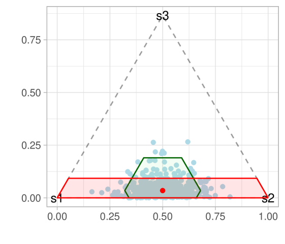
Figure 1: Posterior samples of $\tilde{{\boldsymbol{p}}}$ (blue) and ambiguity sets $\mathcal{P}^{\operatorname{std}}$ (green) and $\mathcal{P}^{\operatorname{opt}}$ (red) from Example 3.3.

The following illustrates how the span along $\hat{{\boldsymbol{z}}}$ impacts the performance loss of the RMDP policy.

Example 3.3.

Consider an MDP with states $\{0,1,2,3\}$ and a single action $\{1\}$. The state $0$ is initial, and the states $1,2,3$ are terminal with $P(i,1,i)=1,i=1,2,3$ with zero rewards. To keep the notation simple, we assume that it is only possible to transition from state $0$ to states $1,2,3$. The transition probability $\tilde{{\boldsymbol{p}}}_{0,1}$ is uncertain and distributed as $\tilde{{\boldsymbol{p}}}_{0,1}\sim\operatorname{Dirichlet}(10,10,1)$ with $\mathbb{E}[\tilde{{\boldsymbol{p}}}_{0,1}]=[0.48,0.48,0.04]$. The rewards are ${\boldsymbol{r}}_{0,1}=[0.25,0.25,-1]$. The goal is to maximize the percentile criterion with $\delta=0.2$.

Take the MDP from Example 3.3 and construct RMDPs with the following two ambiguity sets depicted in Figure 1. Let $\mathcal{P}^{\operatorname{std}}=\mathcal{P}_{1,1}(\nicefrac{{1}}{{\sqrt{3}}}\cdot\bm{1},0.1)$ be the standard ambiguity set with uniform weights, and let $\mathcal{P}^{\operatorname{opt}}=\mathcal{P}_{1,1}(\nicefrac{{1}}{{\sqrt{1.12}}}\cdot[0.25,0.25,1],0.1)$ be an ambiguity set with optimized weights ${\boldsymbol{w}}=\nicefrac{{1}}{{\sqrt{1.12}}}\cdot[0.25,0.25,1]$. The budgets for both ambiguity sets are minimally sufficient to satisfy 1. Intuitively, this means that at least $80\%$ of the posterior samples of $\tilde{{\boldsymbol{p}}}_{0,1}$ (blue dots in Figure 1) must be contained inside of each ambiguity set. Now, with $80\%$ confidence, the RMDP with $\mathcal{P}^{\operatorname{opt}}$ guarantees return $\hat{\rho}^{\operatorname{opt}}=0.16$, while the RMDP with $\mathcal{P}^{\operatorname{std}}$ guarantees only $\hat{\rho}^{\operatorname{std}}=-0.06$. Although the volumes of $\mathcal{P}^{\operatorname{std}}$ and $\mathcal{P}^{\operatorname{opt}}$ are approximately equal, the span along the dimension ${\boldsymbol{z}}=[0.25,0.25,-1]$ of $\mathcal{P}^{\operatorname{opt}}$ is half of the span of $\mathcal{P}^{\operatorname{std}}$.

Input: Confidence $1-\delta$, posterior distribution $f$ over $\tilde{P}$

Output: Ambiguity set $\mathcal{P}({\boldsymbol{w}},\psi)$

1 Compute ${\boldsymbol{v}}^{\prime}\in\mathbb{R}^{S}$ by solving $\max_{\pi}\;\rho\bigl{(}\pi,\mathbb{E}\bigl{[}\tilde{P}\bigr{]}\bigr{)}$ and let ${\boldsymbol{z}}^{\prime}_{s,a}\leftarrow{\boldsymbol{r}}_{s,a}+\gamma\cdot{\boldsymbol{v}}^{\prime},\,s\in\mathcal{S},a\in\mathcal{A}$;

Compute minimal $\psi^{\prime}:\mathcal{S}\times\mathcal{A}\to\mathbb{R}_{+}$ such that 1 holds for $\mathcal{P}(\nicefrac{{1}}{{\sqrt{S}}}\cdot\bm{1},\psi^{\prime})$;

  // Algorithm 3

Compute ${\boldsymbol{w}}_{s,a}\leftarrow\min_{{\boldsymbol{w}}\in\mathbb{R}^{S}_{+}}\;\{\beta_{{\boldsymbol{z}}^{\prime}}^{s,a}({\boldsymbol{w}},\psi^{\prime})\;|\;\left\lVert{\boldsymbol{w}}\right\rVert_{2}=1\}$ for each $s\in\mathcal{S}$, $a\in\mathcal{A}$;

  // Algorithm 2

Compute minimal $\psi:\mathcal{S}\times\mathcal{A}\to\mathbb{R}_{+}$ such that 1 holds for $\mathcal{P}({\boldsymbol{w}},\psi)$;

  // Algorithm 3

return Ambiguity set $\mathcal{P}({\boldsymbol{w}},\psi)$

Algorithm 1 Ambiguity shape optimization scheme.

Armed with the safety and performance loss guarantees in Theorems 3.1 and 3.2, we propose a new heuristic algorithm in Algorithm 1 which iteratively optimizes the shape of the ambiguity set in order to improve the guaranteed percentile. It constructs ambiguity sets that minimize the span of the ambiguity set. The algorithm may not construct the optimal ambiguity set because it first uses the nominal value function ${\boldsymbol{v}}^{\prime}$. However, the algorithm provides guarantees on the quality of the policy that it computes from 1 and Theorems 3.1 and 3.2.

4 Minimizing Ambiguity Spans

This section describes tractable algorithms that optimize the weights ${\boldsymbol{w}}$ to minimize that span $\beta_{{\boldsymbol{z}}}^{s,a}$ for some fixed state $s\in\mathcal{S}$, action $a\in\mathcal{A}$, a vector ${\boldsymbol{z}}\in\mathbb{R}^{S}$, and a budget $\psi\in\mathbb{R}_{+}$. We describe an analytical solution and a conic formulation that minimize an upper bound on the span for weighted $L_{1}$ and $L_{\infty}$ sets. The budget $\psi$ is fixed throughout this section; Section 5 describes how to optimize it.

The goal of computing the weights ${\boldsymbol{w}}$ that minimize the span of the ambiguity set for a fixed budget $\psi$ can be formalized as the following optimization problem:

$$\min_{{\boldsymbol{w}}\in\mathbb{R}^{S}_{+}}\;\Bigl{\{}\beta_{{\boldsymbol{z}}}^{s,a}({\boldsymbol{w}},\psi)\;|\;\left\lVert{\boldsymbol{w}}\right\rVert_{2}=1\Bigr{\}}.$$ (6)

The optimization in (6) is not obviously convex, but we propose methods that minimize an upper bound on $\beta_{{\boldsymbol{z}}}^{s,a}({\boldsymbol{w}},\psi)$. Note that minimizing this upper bound also minimizes an upper bound on Theorem 3.2.

We first describe two analytical solutions and then describe a more precise but also more computationally intensive method based on second order conic approximation. The following lemma provides a bound that enables efficient optimization.

Lemma 4.1.

The span $\beta_{{\boldsymbol{z}}}^{s,a}$ of the ambiguity set $\mathcal{P}_{s,a}({\boldsymbol{w}},\psi)$ is bounded for any $\lambda\in\mathbb{R}$ as:

$$\beta_{{\boldsymbol{z}}}^{s,a}({\boldsymbol{w}},\psi) \leq 2\cdot\psi\cdot\left\lVert{\boldsymbol{z}}-\lambda\cdot{\boldsymbol{1}}\right\rVert_{\star}~{},$$ (7)

where $\left\lVert\cdot\right\rVert_{\star}$ is the norm dual to $\left\lVert\cdot\right\rVert_{{\boldsymbol{w}}}$.

The proof is deferred to Section A.2. Recall that the dual norm is defined as $\left\lVert{\boldsymbol{c}}\right\rVert_{\star}=\max_{{\boldsymbol{x}}\in\mathbb{R}^{S}}\,\left\{{\boldsymbol{c}}^{\mkern-1.5mu\mathsf{T}}{\boldsymbol{x}}\;|\;\left\lVert{\boldsymbol{x}}\right\rVert\leq 1\right\}$.

In order to use the bound in Lemma 4.1, we need to derive the dual norms to the weighted $L_{1}$ and weighted $L_{\infty}$ norms. For unweighted $p$-norms, it is well known that $L_{1}$ and $L_{\infty}$ norms are dual of each other, but we are not aware of a similar result for their weighted variants. The following lemma establishes that weighted $L_{1}$ and $L_{\infty}$ norms are dual as long as their weights are inverse elementwise.

Lemma 4.2.

Suppose that ${\boldsymbol{w}}\in\mathbb{R}^{S}$ and ${\boldsymbol{w}}^{\prime}\in\mathbb{R}^{S}$ are positive $w_{i}>0,w_{i}^{\prime}>0$ and satisfy that $w_{i}^{\prime}=\nicefrac{{1}}{{w_{i}}}$ for all $i\in\mathcal{S}$. Then:

$$\left\lVert{\boldsymbol{z}}\right\rVert_{\infty,{\boldsymbol{w}}^{\prime}}\;=\;\max_{{\boldsymbol{x}}\in\mathbb{R}^{S}}\,\left\{{\boldsymbol{z}}^{\mkern-1.5mu\mathsf{T}}{\boldsymbol{x}}\;|\;\left\lVert{\boldsymbol{x}}\right\rVert_{1,{\boldsymbol{w}}}=1\right\}.$$

The proof of the lemma can be found in Section A.2.

Input: Norm $q\in\{1,\infty\}$, parameter $\lambda\in\mathbb{R}$

Output: Weights ${\boldsymbol{w}}^{\star}\in\mathbb{R}_{+}^{S}$ that minimize (7)

1 if $q=1$ then

2       $w_{i}^{\star}\leftarrow\frac{\lvert z_{i}-\lambda\rvert^{1/3}}{\sqrt{\sum_{j=1}^{S}{\lvert z_{j}-\lambda\rvert^{2/3}}}},\,\forall i\in\mathcal{S}$ ;

3      

4 else if $q=\infty$ then

5       $w_{i}^{\star}\leftarrow\frac{\lvert z_{i}-\lambda\rvert}{\sqrt{\sum_{j=1}^{S}\lvert z_{j}-\lambda\rvert^{2}}},\,\forall i\in\mathcal{S}$ ;

6      

7 end if

8return ${\boldsymbol{w}}^{\star}$ ;

Algorithm 2 Weight optimization.

Based on the results above, Algorithm 2 summarizes our algorithms for computing weights ${\boldsymbol{w}}$ that minimize the upper bound on the performance loss in Theorem 3.2. The algorithm runs in linear time. Note that the algorithm assumes that a value of $\lambda$ is given. Although it would be possible to optimize for the best value of $\lambda$, our preliminary experimental results suggest that this is not worthwhile because it does not lead to a significant improvement. Instead, we use $\lambda=(\max_{i}z_{i}+\min_{i}z_{i})/2$ and $\lambda=\operatorname{median}({\boldsymbol{z}})$ for $L_{\infty}$ and $L_{1}$ norms respectively. These are the optimal values (values for which the upper bound is smallest) for the uniform weight version of (7). The following proposition states the correctness of this algorithm.

Proposition 4.3.

Fix an arbitrary $\lambda\in\mathbb{R}$ and let ${\boldsymbol{w}}^{\star}\in\mathbb{R}_{+}^{S}$ the return from Algorithm 2. Then ${\boldsymbol{w}}^{\star}$ is an optimal solution to (7) weighted $L_{1}$ and $L_{\infty}$ norms.

Please see Section A.2 for the proof.

It is important to recognize that even though Algorithm 2 effectively minimizes the value $\beta^{s,a}_{{\boldsymbol{z}}}$, it may, in the process, violate 1. This is because scaling weights may reduce the probability that $\tilde{P}\in\mathcal{P}$. We are not aware of a tractable algorithm that can optimize the weights ${\boldsymbol{w}}$ directly while enforcing the constraint of 1. Instead, the constraint $\left\lVert{\boldsymbol{w}}\right\rVert_{2}=\psi$ serves as a proxy to prevent the ambiguity from shrinking. This is why it is necessary to re-optimize the budget $\psi$ in Algorithm 1 after the weights are optimized.

As an alternative to the analytical algorithms in Algorithm 2, we also examine a Second-Order Conic Program (SOCP) formulation. This formulation optimizes a tighter upper bound on $\beta^{s,a}_{{\boldsymbol{z}}}$ but is more computationally intensive. For any fixed state $s$ and action $a$, the following SOCP minimizes the bound (7) on $\beta_{{\boldsymbol{z}}}^{s,a}({\boldsymbol{w}},\psi)$ for the $L_{1}$ norm:

$$\begin{array}[]{>{\displaystyle}l>{\displaystyle}l>{\displaystyle}l}\operatorname*{minimize}_{{\boldsymbol{g}},c,\lambda}&\psi\cdot c\\[4.30554pt] \operatorname{subject\,to}&{\boldsymbol{g}}\;\geq\;\max\{{\boldsymbol{z}}-\lambda\cdot\bm{1},-{\boldsymbol{z}}+\lambda\cdot\bm{1}\}\\[4.30554pt] &{\boldsymbol{g}}^{\mkern-1.5mu\mathsf{T}}{\boldsymbol{g}}\;\leq\;c^{2},\quad{\boldsymbol{g}}\;\geq\;\bm{0}~{}.\end{array}$$ (8)

The SOCP formulation follows from Lemma 4.2 and variable substitution ${\boldsymbol{g}}={\boldsymbol{w}}\cdot c$.

Remark 4.4 (Unreachable states).

We assume that the prior can specify some transitions as impossible, or unreachable: that is $P(s,a,s^{\prime})=0$. This information is used as an additional pre-processing step in optimizing the weights. In particular, if the transition from state $s$ after taking action $a$ to state $s^{\prime}$ is not possible, then we set $({\boldsymbol{w}}_{s,a})_{s^{\prime}}=\infty$. Or, in other words, each ${\boldsymbol{p}}\in\mathcal{P}_{s,a}({\boldsymbol{w}},\psi)$ satisfies $p_{s^{\prime}}=0$.

5 Minimizing Ambiguity Budgets

This section describes how to determine the size of the ambiguity set in the Bayesian setting in order to minimize the performance loss in Theorem 3.2 of the RMDP policy while satisfying 1. We assume that the weights ${\boldsymbol{w}}_{s,a},s\in\mathcal{S},a\in\mathcal{A}$ are arbitrary but fixed and aim to construct $\psi_{s,a},s\in\mathcal{S},a\in\mathcal{A}$ to minimize the performance loss.

Before describing the algorithm, we state a simple observation that motivates its construction. The following lemma implies that the smaller the ambiguity budget is, the better $\hat{\rho}$ approximates the percentile criterion. Of course, this is only true as long as the budget is sufficiently large for 1 to hold. The following proposition follows from the definition of $\beta^{s,a}_{{\boldsymbol{z}}}$ by algebraic manipulation.

Lemma 5.1.

The function $\psi\mapsto\beta^{s,a}_{{\boldsymbol{z}}}({\boldsymbol{w}}_{s,a},\psi)$ is non-decreasing.

Input: Posterior samples $P_{1},\ldots,P_{n}$ from $\tilde{P}$, weights ${\boldsymbol{w}}_{s,a}$, norm $q\in\{1,\infty\}$

Output: Nominal $\bar{{\boldsymbol{p}}}_{s,a}$ and budget $\psi_{s,a}$

1 Compute nominal $\bar{{\boldsymbol{p}}}_{s,a}\leftarrow(1/n)\sum_{i=1}^{n}P_{i}(s,a)$ ;

2 Compute distance $d_{i}\leftarrow\left\lVert P_{i}(s,a)-\bar{{\boldsymbol{p}}}_{s,a}\right\rVert_{q,{\boldsymbol{w}}_{s,a}}$ ;

3 Ascending sort: $d_{(j)}\leq d_{(j+1)},\,j=1,\ldots,n$;

4 Compute the quantile $\psi_{s,a}\leftarrow d_{(\lceil(1-\delta/(S\cdot A))\cdot n\rceil)}$ ;

return $\bar{{\boldsymbol{p}}}_{s,a}$ and $\psi_{s,a}$

Algorithm 3 Budget optimization.

We are now ready to describe our method as outlined in Algorithm 3. The algorithm follows the well-known sample average approximation (SAA) approach common in stochastic programming Shapiro et al., (2014). It constructs ambiguity sets as credible regions for the posterior distribution over $\tilde{P}$ similarly to prior work (Petrik and Russel,, 2019). The next proposition states the correctness of Algorithm 3.

Proposition 5.2.

Suppose that $\psi_{s,a}$ are computed by Algorithm 3 for some ${\boldsymbol{w}}_{s,a}$ for each $s\in\mathcal{S}$ and $a\in\mathcal{A}$. Also let $w:(s,a)\mapsto{\boldsymbol{w}}_{s,a}$ and $\psi:(s,a)\mapsto\psi_{s,a}$. Then $\mathcal{P}(w,\psi)$ satisfies 1 with high probability when a sufficient number of samples from $\tilde{P}$ are used.

Please see Section A.3 for the proof.

Algorithm 3 constructs credible regions for each state and action separately (Murphy,, 2012). A notable limitation of Algorithm 3 is that it constructs the credible regions independently for each state and action. Although this is convenient computationally, it also means that the confidence region needs to rely on the union bound which makes it the impractical when the number of states and actions is large. Although, 1 allows for a construction that avoids the union-bound-based construction.

While Proposition 5.2 provides asymptotic convergence guarantees, it is possible to obtain finite sample guarantee by using more careful analysis Luedtke and Ahmed, (2008) or by adapting Algorithm 3 as suggested in Hong et al., (2020). We leave this finite-sample analysis for future work.

6 Frequentist Guarantees

In this section, we extend the analysis above to outline how our results apply to frequentist guarantees. The advantage of the frequentist setup is that it provides guarantees even without needing access to a prior distribution. The disadvantage is that, without good priors, frequentist settings may need an excessive amount of data to provide reasonable guarantees. The main contribution in this section are new sampling bounds for weighted $L_{1}$ and $L_{\infty}$ ambiguity sets.

The frequentist perspective on the percentile criterion Delage and Mannor, (2010) represents a viable alternative to the Bayesian perspective when it is difficult to construct a good prior distribution. The frequentist view assumes that the true model $P^{\star}$ is known. The analysis considers the uncertainty over datasets. To define the criterion, let $\mathcal{D}$ represent the set of all possible datasets $D$. Then the pair of algorithms $F:\mathcal{D}\to\Pi$, which computes the policy for a dataset, and $G:\mathcal{D}\to\mathbb{R}$, which estimates the return of the policy, solves the percentile criterion if:

$$\mathbb{P}_{D\sim P^{\star}}\left[\rho(F(D),P^{\star})\geq G(D)\right]\;\geq\;1-\delta~{}.$$ (9)

A frequentist modeler assumes that $P^{\star}_{s,a}$ is fixed and the probability statements are qualified over sampled data sets $(s_{t},a_{t},s_{t}^{\prime})_{t=1,\ldots,T}$ generated from the true transition probabilities $s_{t}^{\prime}\sim{\boldsymbol{p}}^{\star}_{s_{t},a_{t}}$.

To construct an RMDP that solves the frequentist percentile criterion, we make very similar assumptions to the Bayesian setting. The next assumption restates 1 in the frequentist setting; note the change in random variables.

Assumption 2.

The data-dependent ambiguity set $\hat{\mathcal{P}}$ satisfies:

$$\mathbb{P}_{D\sim P^{\star}}\bigl{[}P^{\star}\in\hat{\mathcal{P}}\bigr{]}\;\geq\;1-\delta\,,$$

where $\hat{\mathcal{P}}$ is a function of $D$.

Recall that Theorem 3.1 establishes that an RMDP that satisfies 1 computes a high-confidence lower bound on the return. The proof of Theorem 3.1 easily extends to the frequentist setup. Therefore, 2 implies that $\mathbb{P}_{D}\left[\hat{\rho}\leq\rho(\hat{\pi},P)\right]\geq 1-\delta$ where $\hat{\rho}$ and $\hat{\pi}$ are the return and policy to the RMDP. In other words, the RMDP algorithm (joint policy and return estimate computation) solves the frequentist percentile criterion in (9) when 2 holds.

Because the optimization methods described in Section 4 make no probabilistic assumptions, they can be applied to the frequentist setup with no change. The optimization of $\psi$ described in Section 5 assumes that samples from the posterior over transition functions are available and cannot be readily used to satisfy 2. Instead, we present two new finite-sample bounds that can be used to construct frequentist ambiguity sets. Since prior work has been limited to the ambiguity sets defined in terms $L_{1}$ ambiguity sets with uniform weights (Weissman et al.,, 2003; Auer et al.,, 2010; Dietterich et al.,, 2013; Petrik and Russel,, 2019), we derive new high-confidence bounds for ambiguity sets defined using weighted $L_{1}$ and $L_{\infty}$ norms. To state our new results, let the nominal point $\bar{{\boldsymbol{p}}}_{s,a}\in\Delta^{S}$ in (3) be the empirical estimate of the transition probability computed from $n_{s,a}\in\mathbb{N}$ transition samples for each state $s\in\mathcal{S}$ and action $a\in\mathcal{A}$.

Theorem 6.1 ($L_{\infty}$ norm).

Suppose that $\mathcal{P}({\boldsymbol{w}},\psi)$ is defined in terms of the ${\boldsymbol{w}}_{s,a}$-weighted $L_{\infty}$ norm. Then 2 is satisfied if $\psi_{s,a}\in\mathbb{R}_{+}$ for each $s\in\mathcal{S}$ and $a\in\mathcal{A}$ satisfies the following inequality:

$$\delta\;\leq\;2\cdot SA\cdot\sum_{i=1}^{S}\exp\left(-2\frac{\psi_{s,a}^{2}\cdot n_{s,a}}{({\boldsymbol{w}}_{sa})_{i}^{2}}\right)~{}.$$ (10)

Theorem 6.2 ($L_{1}$ norm).

Suppose that $\mathcal{P}({\boldsymbol{w}},\psi)$ is defined in terms of the ${\boldsymbol{w}}_{s,a}$-weighted $L_{1}$ norm. Then 2 is satisfied if $\psi_{s,a}\in\mathbb{R}_{+}$ for each $s\in\mathcal{S}$ and $a\in\mathcal{A}$ satisfies the following inequality:

$$\delta\;\leq\;2\cdot SA\cdot\sum_{i=1}^{S-1}2^{S-i}\cdot\exp\left(-\frac{\psi_{s,a}^{2}\cdot n_{s,a}}{2\cdot({\boldsymbol{w}}_{sa})_{i}^{2}}\right)~{},$$ (11)

where positive weights ${\boldsymbol{w}}_{s,a}\in_{++}^{S},s\in\mathcal{S},a\in\mathcal{A}$ are assumed to be sorted in a non-increasing order $({\boldsymbol{w}}_{s,a})_{i}\geq({\boldsymbol{w}}_{s,a})_{i+1}$ for $i=1,\ldots,S-1$.

The proofs of the theorems are in Section A.4. They follow by standard techniques combining the Hoeffding and union bounds.

A natural question is how to construct $\psi_{s,a}$ that satisfies Theorems 6.1 and 6.2. Although the theorems do not provide us with an analytical solution, the value of $\psi_{s,a}$ can be computed efficiently using the standard bisection method Boyd and Vandenberghe, (2004). This is because right-hand side functions in (10) and (11) are monotonically decreasing in $\psi_{s,a},s\in\mathcal{S},a\in\mathcal{A}$. Theorem A.3 further tightens the error bounds using Bernstein’s inequality.

Theorems 6.1 and 6.2 also provide new insights into which ambiguity set may be a better fit for a particular problem. Simple algebraic manipulation and (7) show that the $L_{1}$ norm is preferable to the $L_{\infty}$ norm when $\left\lVert{\boldsymbol{v}}-\bar{v}\cdot\bm{1}\right\rVert_{1}>\sqrt{S}\cdot\left\lVert{\boldsymbol{v}}-\tilde{v}\cdot\bm{1}\right\rVert_{\infty}$. Here, ${\boldsymbol{v}}\in\mathbb{R}^{S}$ is the optimal value function, $\bar{v}=\bm{1}^{\mkern-1.5mu\mathsf{T}}{\boldsymbol{v}}/S$ is the mean value, and $\tilde{v}$ is the median value of ${\boldsymbol{v}}$.

In terms of their tightness, Theorems 6.1 and 6.2 are similar to the most well-known bounds on the uniformly-weighted norms. Theorem 6.2 recovers the equivalent best-known (Hoeffding-based) result for uniformly-weighted norm within a factor of $2$. We are not aware of comparable prior results for ambiguity sets defined in terms of $L_{\infty}$ norms. Unfortunately, frequentist bounds on probability distributions are generally useful only when the number of samples $n_{s,a}$ is quite large. We also investigated Bernstein-based versions of the bounds, but they show little difference in our experimental results.

Finally, it is important to note that Theorems 6.1 and 6.2 require that the weights ${\boldsymbol{w}}$ are independent of data. Therefore, the weights ${\boldsymbol{w}}$ should be optimized using a dataset different from the one used to estimate $\psi$. However, in our experiment, we found that reusing the same dataset to optimize both ${\boldsymbol{w}}$ and $\psi$ empirically does compromise the percentile guarantees.

7 Empirical Evaluation

In this section, we evaluate Algorithm 1 empirically using five standard reinforcement domains that have been previously used to evaluate robustness.

Tables 1 and 2 summarize the results for the Bayesian and frequentist setups respectively. The results compare our algorithms (rows) against baselines (rows) for fixed datasets $D$ for all domains (column). The method names indicate how the weights are computed and which norm is used to defined the ambiguity set. Methods denoted as “Uniform” represent ${\boldsymbol{w}}=\bm{1}$ and “Optimized” represent ${\boldsymbol{w}}$ computed using Algorithms 1 and 2. Please see Appendix B for a complete report of the statistics and methods (including the SOCP formulation).

As the main metric, we compare the computed return guarantees $\hat{\rho}$ (the return of the RMDP). Because all methods use ambiguity sets that satisfy 1 and 2, $\hat{\rho}$ lower bounds $\rho(\hat{\pi},\tilde{P})$ with probability $1-\delta$. In order to enable the comparison of the results among different domains, we normalize the guarantee by the maximal nominal return $\bar{\rho}=\max_{\pi\in\Pi}\rho(\pi,\mathbb{E}[\tilde{P}])$. We use $\bar{\rho}$ instead of the unknown $y^{\star}$.

As a baseline, we compare our results with the standard RMDPs construction Petrik and Russel, (2019); Delage and Mannor, (2010), which uses uniformly-weighted $L_{1}$ and $L_{\infty}$ norms. We do not compare to policy-gradient-style methods in Delage and Mannor, (2010) because they cannot be used with general posterior distributions over $\tilde{P}$ in our domains. We note that various modifications to probability norms have been proposed in the RL context (e.g., Maillard et al., (2014); Taleghan et al., (2015)), but it is unclear how to use them in the context of the percentile criterion.

The results in Tables 1 and 2 show that optimizing the weights in RMDP ambiguity sets decreases the guaranteed performance loss dramatically in Bayesian settings (geometric mean $2.8\times$) and reliably in frequentist settings (geometric mean $1.6\times$). The guarantees improve because the RMDPs with optimized sets simultaneously compute a better policy and a tighter bound on its return. Note that zero losses in the tables may be unachievable ($\bar{\rho}>y^{\star}$), and losses greater than one are possible (when $\bar{\rho}<0$). The total computational complexity of Algorithms 1 and 2 is small and reported in Appendix B.

We now briefly summarize the domains used; please consult Appendix B for more details.

RiverSwim (RS) is a simple and standard benchmark (Strehl and Littman,, 2008), which is an MDP consisting of six states and two actions. The process follows by sampling synthetic datasets from the true model and then computing the guaranteed robust returns for different methods. The prior is a uniform Dirichlet distribution over reachable states.

Machine Replacement (MR) is a small benchmark MDP problem with $S=10$ states that models progressive deterioration of a mechanical device Delage and Mannor, (2010). Two repair actions $A=2$ are available and restore the machine’s state. Uses a Dirichlet prior.

Population Growth Model (PG) is an exponential population growth model (Kéry and Schaub,, 2011), which constitutes a simple state-space $0,\ldots,S=50$ with exponential dynamics. At each time step, the land manager has to decide whether to apply a control measure to reduce the species’ growth rate. We refer to Tirinzoni et al., (2018) for more details of the model.

Inventory Management (IM) is a classic inventory management problem (Zipkin,, 2000), with discrete inventory levels $0,\ldots,S=30$. The purchase cost, sale price, and holding cost are $2.49,3.99$, and $0.03$, respectively. The demand is sampled from a normal distribution with a mean $S/4$ and a standard deviation of $S/6$. It also uses a Dirichlet prior.

Cart-Pole (CP) is the standard RL benchmark problem (Sutton and Barto,, 2018; Brockman et al.,, 2016). We collect samples of $100$ episodes from the true dynamics. We fit a linear model with that dataset to generate synthetic samples and aggregate close states to a 200-cell grid ($S=200$) using the k-nearest neighbor strategy and assume a uniform Dirichlet prior.

	RS	MR	PG	IM	CP
Uniform $L_{1}$	0.60	1.56	5.24	0.97	0.77
Uniform $L_{\infty}$	0.60	1.56	5.50	0.98	0.76
Optimized $L_{1}$	0.25	0.41	1.84	0.90	0.12
Optimized $L_{\infty}$	0.31	0.39	3.10	0.87	0.19

Table 1: Normalized Bayesian performance loss $(\bar{\rho}-\hat{\rho})/|\bar{\rho}|$ for $\delta=0.05$. (Smaller value is better).

	RS	MR	PG	IM	CP
Uniform $L_{1}$	0.80	5.83	5.66	1.05	0.78
Uniform $L_{\infty}$	0.76	3.45	5.65	1.05	0.78
Optimized $L_{1}$	0.53	1.05	5.55	0.99	0.77
Optimized $L_{\infty}$	0.43	0.94	5.56	0.96	0.69

Table 2: Normalized frequentist performance loss $(\bar{\rho}-\hat{\rho})/|\bar{\rho}|$ for $\delta=0.05$. (Smaller value is better).

8 Conclusion

We proposed a new approach for optimizing the percentile criterion using RMDPs that goes beyond the conventional ambiguity sets. At the heart of our method are new bounds on the performance loss of the RMDPs with respect to the optimal percentile criterion. These bounds show that the quality of the RMDP is driven by the span of its ambiguity sets along a specific direction. We proposed a linear-time algorithm that minimizes the span of the ambiguity sets and also derived new sampling guarantees. Our experimental results show that this simple RMDP improvement can lead to much better return guarantees. Future work needs to focus on scaling the method to a large state-space using value function approximation or other techniques.

Acknowledgments

We thank the anonymous reviewers for comments that helped to improve this paper. This work was supported, in part, by the National Science Foundation (Grants IIS-1717368 and IIS-1815275), the CityU Start-up Grant (Project No. 9610481), the CityU Strategic Research Grant (Project No. 7005534), and the National Natural Science Foundation of China (Project No. 72032005). Any opinion, finding, and conclusion or recommendation expressed in this material are those of the authors and do not necessarily reflect the views of the National Science Foundation and the National Natural Science Foundation of China.

Appendix A Technical Results and Proofs

A.1 Proofs of Results in Section 3

Proof of Theorem 3.1.

The result can be derived as:

$$\mathbb{P}_{\tilde{P}\sim f}\left[\hat{\rho}\leq\rho(\hat{\pi},\tilde{P})\right] \stackrel{{\scriptstyle\text{(a)}}}{{=}}\mathbb{P}_{\tilde{P}\sim f}\left[\rho(\hat{\pi},\tilde{P})\geq\max_{\pi\in\Pi}\min_{P\in\hat{\mathcal{P}}}\rho(\pi,P)\right]$$

$$\stackrel{{\scriptstyle\text{(b)}}}{{=}}\mathbb{P}_{\tilde{P}\sim f}\left[\rho(\hat{\pi},\tilde{P})\geq\min_{P\in\hat{\mathcal{P}}}\rho(\hat{\pi},P)\right]$$

$$\stackrel{{\scriptstyle\text{(c)}}}{{\geq}}\mathbb{P}_{\tilde{P}\sim f}\left[\tilde{P}\in\hat{\mathcal{P}}\right]\stackrel{{\scriptstyle\text{(d)}}}{{\geq}}1-\delta~{}.$$

The equality (a) follows from the definition of $\hat{\rho}$, the inequality (b) follows from $\hat{\pi}\in\Pi$ and is optimal, (c) follows because $\rho(\hat{\pi},\tilde{P})\geq\min_{P\in\hat{\mathcal{P}}}\rho(\hat{\pi},P)$ whenever $\tilde{P}\in\hat{\mathcal{P}}$, and (d) follows from the theorem’s hypothesis. ∎

Proof of Theorem 3.2.

Let $\hat{\mathcal{P}}=\mathcal{P}({\boldsymbol{w}},\psi)$ and let $\hat{\rho}$ and $\hat{\pi}$ be the optimal return and policy for $\hat{\mathcal{P}}$ respectively. We start by establishing the following bound:

$$\hat{\rho}\geq\max_{\pi\in\Pi}\rho(\pi,\tilde{P})-\frac{\beta_{\hat{{\boldsymbol{z}}}}({\boldsymbol{w}},\psi)}{1-\gamma}~{},$$

where

$$\beta_{\hat{{\boldsymbol{z}}}}({\boldsymbol{w}},\psi)=\max_{s\in\mathcal{S}}\max_{a\in\mathcal{A}}\,\beta^{s,a}_{\hat{{\boldsymbol{z}}}}({\boldsymbol{w}},\psi)~{}.$$

Let $\hat{{\boldsymbol{v}}}\in\mathbb{R}^{S}$ be the optimal robust value function that satisfied $\hat{{\boldsymbol{v}}}=\mathfrak{L}\hat{{\boldsymbol{v}}}$ for the ambiguity set $\hat{\mathcal{P}}=\mathcal{P}({\boldsymbol{w}},\psi)$. We use $\hat{\mathcal{P}}$ as a shorthand for $\mathcal{P}({\boldsymbol{w}},\psi)$ throughout the proof. Recall that $\hat{\rho}={\boldsymbol{p}}_{0}^{\mkern-1.5mu\mathsf{T}}\hat{{\boldsymbol{v}}}$. We also use $\mathfrak{T}_{\pi}^{P}$ to represent the Bellman evaluation operator for a policy $\pi\in\Pi$ and a transition function $P$ defined for each $s\in\mathcal{S}$ as:

$$(\mathfrak{T}_{\pi}^{P}\,v)_{s}=P(s,\pi(s))^{\mkern-1.5mu\mathsf{T}}({\boldsymbol{r}}_{s,a}+\gamma\cdot{\boldsymbol{v}})~{}.$$

It is well known that $\mathfrak{T}_{\pi}^{P}\,v$ is a contraction, is monotone, and has a unique fixed point. Let $\tilde{v}$ be the unique fixed point of $\mathfrak{T}_{\tilde{\pi}}^{\tilde{P}}$:

$$\tilde{{\boldsymbol{v}}}=\mathfrak{T}_{\tilde{\pi}}^{\tilde{P}}\tilde{{\boldsymbol{v}}}~{},$$

where $\tilde{\pi}\in\arg\max_{\pi\in\Pi}\,\rho(\pi,\tilde{P})$. Note that it is well known that:

$${\boldsymbol{p}}_{0}^{\mkern-1.5mu\mathsf{T}}\tilde{{\boldsymbol{v}}}=\rho(\tilde{\pi},\tilde{P})~{}.$$

Now suppose that $\tilde{P}\in\hat{\mathcal{P}}$, which holds with probability $1-\delta$ according to 1. Then it is easy to see that:

$${\boldsymbol{p}}_{0}^{\mkern-1.5mu\mathsf{T}}\hat{{\boldsymbol{v}}}=\min_{P\in\hat{\mathcal{P}}}\rho(\pi,P)\leq\rho(\pi,\tilde{P})\leq{\boldsymbol{p}}_{0}^{\mkern-1.5mu\mathsf{T}}\tilde{{\boldsymbol{v}}}~{}.$$

Therefore:

$$0\leq{\boldsymbol{p}}_{0}^{\mkern-1.5mu\mathsf{T}}\tilde{{\boldsymbol{v}}}-{\boldsymbol{p}}_{0}^{\mkern-1.5mu\mathsf{T}}\hat{{\boldsymbol{v}}}\leq\left\lVert\tilde{{\boldsymbol{v}}}-\hat{{\boldsymbol{v}}}\right\rVert_{\infty}~{}.$$

We are now ready to establish the probabilistic bound which is based on bounding the Bellman residual as follows:

$$(\mathfrak{T}_{\tilde{\pi}}^{\tilde{P}}\hat{{\boldsymbol{v}}}-\hat{{\boldsymbol{v}}})_{s} \stackrel{{\scriptstyle\text{(a)}}}{{=}}(\mathfrak{T}_{\tilde{\pi}}^{\tilde{P}}\hat{{\boldsymbol{v}}}-\mathfrak{L}\hat{{\boldsymbol{v}}})_{s}\stackrel{{\scriptstyle\text{(def)}}}{{=}}\tilde{P}(s,\tilde{\pi}(a))^{\mkern-1.5mu\mathsf{T}}\hat{{\boldsymbol{z}}}_{s,\tilde{\pi}(s)}-\min_{P\in\hat{\mathcal{P}}}P(s,\hat{\pi}(a))^{\mkern-1.5mu\mathsf{T}}\hat{{\boldsymbol{z}}}_{s,\hat{\pi}(a)}$$

$$\stackrel{{\scriptstyle\text{(b)}}}{{\leq}}\tilde{P}(s,\tilde{\pi}(a))^{\mkern-1.5mu\mathsf{T}}\hat{{\boldsymbol{z}}}_{s,\tilde{\pi}(s)}-\min_{P\in\hat{\mathcal{P}}}P(s,\tilde{\pi}(a))^{\mkern-1.5mu\mathsf{T}}\hat{{\boldsymbol{z}}}_{s,\tilde{\pi}(a)}$$

$$\leq\max_{a\in\mathcal{A}}\left(\tilde{P}(s,a)^{\mkern-1.5mu\mathsf{T}}\hat{{\boldsymbol{z}}}_{s,a}-\min_{P\in\hat{\mathcal{P}}}P(s,a)^{\mkern-1.5mu\mathsf{T}}\hat{{\boldsymbol{z}}}_{s,a}\right)$$

$$\stackrel{{\scriptstyle\text{(c)}}}{{\leq}}\max_{a\in\mathcal{A}}\left(\max_{P\in\hat{\mathcal{P}}}P(s,a)^{\mkern-1.5mu\mathsf{T}}\hat{{\boldsymbol{z}}}_{s,a}-\min_{P\in\hat{\mathcal{P}}}P(s,a)^{\mkern-1.5mu\mathsf{T}}\hat{{\boldsymbol{z}}}_{s,a}\right)$$

$$\leq\max_{a\in\mathcal{A}}\,\beta^{s,a}_{\hat{{\boldsymbol{z}}}}({\boldsymbol{w}},\psi)~{}.$$

(a) follows from $\hat{{\boldsymbol{v}}}$ being the fixed point of $\mathfrak{L}$, (b) follows from the optimality of $\hat{\pi}$: $\hat{\pi}(s)\in\arg\max_{a\in\mathcal{A}}\min_{{\boldsymbol{p}}\in\hat{\mathcal{P}}_{s,a}}{\boldsymbol{p}}^{\mkern-1.5mu\mathsf{T}}{\boldsymbol{z}}_{s,a}$, and (c) follows from $\tilde{P}\in\hat{\mathcal{P}}$. The rest follows by algebraic manipulation. Applying the inequality above to all states, we get:

$$\mathfrak{T}_{\tilde{\pi}}^{\tilde{P}}\hat{{\boldsymbol{v}}}-\hat{{\boldsymbol{v}}}\leq\beta_{\hat{{\boldsymbol{z}}}}({\boldsymbol{w}},\psi)\cdot\bm{1}~{}.$$ (12)

We can now use the standard dynamic programming bounding technique to bound $\left\lVert\tilde{{\boldsymbol{v}}}-\hat{{\boldsymbol{v}}}\right\rVert_{\infty}$ as follows:

$$\bm{0}\stackrel{{\scriptstyle\text{(a)}}}{{\leq}}\tilde{{\boldsymbol{v}}}-\hat{{\boldsymbol{v}}}\stackrel{{\scriptstyle\text{(b)}}}{{=}}\tilde{{\boldsymbol{v}}}-\mathfrak{T}_{\tilde{\pi}}^{\tilde{P}}\hat{{\boldsymbol{v}}}+\mathfrak{T}_{\tilde{\pi}}^{\tilde{P}}\hat{{\boldsymbol{v}}}-\hat{{\boldsymbol{v}}}\stackrel{{\scriptstyle\eqref{eq:subopt_bellman}}}{{\leq}}\tilde{{\boldsymbol{v}}}-\mathfrak{T}_{\tilde{\pi}}^{\tilde{P}}\hat{{\boldsymbol{v}}}+\beta_{\hat{{\boldsymbol{z}}}}({\boldsymbol{w}},\psi)\cdot\bm{1}\stackrel{{\scriptstyle\text{(c)}}}{{\leq}}\mathfrak{T}_{\tilde{\pi}}^{\tilde{P}}\tilde{{\boldsymbol{v}}}-\mathfrak{T}_{\tilde{\pi}}^{\tilde{P}}\hat{{\boldsymbol{v}}}+\beta_{\hat{{\boldsymbol{z}}}}({\boldsymbol{w}},\psi)\cdot\bm{1}~{}.$$

We have (a) because $\hat{{\boldsymbol{v}}}\leq\tilde{{\boldsymbol{v}}}$ because $\mathfrak{L}\tilde{{\boldsymbol{v}}}\leq\tilde{{\boldsymbol{v}}}$ and thus $\tilde{{\boldsymbol{v}}}\geq\mathfrak{L}\mathfrak{L}\tilde{{\boldsymbol{v}}}\geq\ldots\geq\mathfrak{L}\ldots\mathfrak{L}\tilde{{\boldsymbol{v}}}\geq\hat{{\boldsymbol{v}}}$ because $\hat{{\boldsymbol{v}}}$ is the fixed point of $\mathfrak{L}$ and $\mathfrak{L}$ is monotone. (b) we add $\bm{0}$, (c) $\tilde{{\boldsymbol{v}}}$ is the fixed point of $\mathfrak{T}_{\tilde{\pi}}^{\tilde{P}}$.

Next, apply $L_{\infty}$ norm to all sides, which is possible because the values are non-negative:

$$\left\lVert\tilde{{\boldsymbol{v}}}-\hat{{\boldsymbol{v}}}\right\rVert_{\infty} \leq\left\lVert\mathfrak{T}_{\tilde{\pi}}^{\tilde{P}}\tilde{{\boldsymbol{v}}}-\mathfrak{T}_{\tilde{\pi}}^{\tilde{P}}\hat{{\boldsymbol{v}}}+\beta_{\hat{{\boldsymbol{z}}}}({\boldsymbol{w}},\psi)\cdot\bm{1}\right\rVert_{\infty}$$

$$\left\lVert\tilde{{\boldsymbol{v}}}-\hat{{\boldsymbol{v}}}\right\rVert_{\infty} \leq\gamma\cdot\left\lVert\tilde{{\boldsymbol{v}}}-\hat{{\boldsymbol{v}}}\right\rVert_{\infty}+\beta_{\hat{{\boldsymbol{z}}}}({\boldsymbol{w}},\psi)$$

$$\left\lVert\tilde{{\boldsymbol{v}}}-\hat{{\boldsymbol{v}}}\right\rVert_{\infty} \leq\beta_{\hat{{\boldsymbol{z}}}}({\boldsymbol{w}},\psi)/(1-\gamma)~{}.$$

The first step follows by triangle inequality, and the second step follows from $\mathfrak{T}_{\tilde{\pi}}^{\tilde{P}}$ being a $\gamma$ contraction in the $L_{\infty}$ norm.

To prove the bound on $y^{\star}$ and $\hat{v}$, we show that $y^{\star}\leq\zeta$ where $\zeta=\hat{\rho}+\beta_{\hat{{\boldsymbol{z}}}}({\boldsymbol{w}},\psi)/(1-\gamma)$. Suppose to the contrary that $y^{\star}>\zeta$. Realize that $y^{\star}$ optimal in (1) must satisfy:

$$\mathbb{P}_{\tilde{P}\sim f}\left[\max_{\pi\in\Pi}\rho(\pi,\tilde{P})\geq y^{\star}\right]\geq 1-\delta~{},$$ (13)

because $\max_{\pi\in\Pi}\rho(\pi,\tilde{P})\geq\rho(\pi^{\star},\tilde{P})$ for $\pi^{\star}$ optimal in (1). Recall also that from the first part of the theorem:

$$\mathbb{P}_{\tilde{P}\sim f}\left[\max_{\pi\in\Pi}\rho(\pi,\tilde{P})\geq\zeta\right]\leq\delta~{}.$$ (14)

We now derive a contradiction as follows:

$$\delta\stackrel{{\scriptstyle\eqref{eq:suboptimal_zeta}}}{{\geq}}\mathbb{P}_{\tilde{P}\sim f}\left[\max_{\pi\in\Pi}\rho(\pi,\tilde{P})\geq\zeta\right]\stackrel{{\scriptstyle\text{(a)}}}{{\geq}}\mathbb{P}_{\tilde{P}\sim f}\left[\max_{\pi\in\Pi}\rho(\pi,\tilde{P})\geq y^{\star}\right]\stackrel{{\scriptstyle\eqref{eq:subopt_ystar}}}{{\geq}}1-\delta~{}.$$

Here (a) follows from the assumption $y^{\star}>\zeta$. Then $\delta\geq 1-\delta$ is a contradiction with $\delta<0.5$. Finally, $0\leq y^{\star}-\hat{\rho}$ follows directly from the optimality of $y^{\star}$ and Theorem 3.1, which proves the theorem. ∎

A.2 Proof of Results in Section 4

Proof of Lemma 4.1.

We omit the $s,a$ subscripts to simplify the notation. By relaxing the non-negativity constraints on ${\boldsymbol{p}}$ and using substitution ${\boldsymbol{q}}_{1}={\boldsymbol{p}}_{1}-\bar{{\boldsymbol{p}}}$ and ${\boldsymbol{q}}_{2}={\boldsymbol{p}}_{2}-\bar{{\boldsymbol{p}}}$, we get the following upper bound:

$$\beta_{{\boldsymbol{z}}}^{s,a}({\boldsymbol{w}},\psi) =\max_{{\boldsymbol{p}}_{1},{\boldsymbol{p}}_{2}}\;\Bigl{\{}({\boldsymbol{p}}_{1}-{\boldsymbol{p}}_{2})^{\mkern-1.5mu\mathsf{T}}{\boldsymbol{z}}\;|\;{\boldsymbol{p}}_{1},{\boldsymbol{p}}_{2}\in\mathcal{P}_{s,a}({\boldsymbol{w}},\psi)\Bigr{\}}$$

$$=\max_{{\boldsymbol{p}}_{1},{\boldsymbol{p}}_{2}}\;\Bigl{\{}({\boldsymbol{p}}_{1}-{\boldsymbol{p}}_{2})^{\mkern-1.5mu\mathsf{T}}{\boldsymbol{z}}\;|\;\left\lVert{\boldsymbol{p}}_{1}-\bar{{\boldsymbol{p}}}\right\rVert_{{\boldsymbol{w}}}\leq\psi,\,\left\lVert{\boldsymbol{p}}_{2}-\bar{{\boldsymbol{p}}}\right\rVert_{{\boldsymbol{w}}}\leq\psi,\,{\boldsymbol{p}}_{1}\in\Delta^{S},\,{\boldsymbol{p}}_{2}\in\Delta^{S}\Bigr{\}}$$

$$\leq\max_{{\boldsymbol{p}}_{1},{\boldsymbol{p}}_{2}\in\mathbb{R}^{S}}\;\Bigl{\{}({\boldsymbol{p}}_{1}-{\boldsymbol{p}}_{2})^{\mkern-1.5mu\mathsf{T}}{\boldsymbol{z}}\;|\;\left\lVert{\boldsymbol{p}}_{1}-\bar{{\boldsymbol{p}}}\right\rVert_{{\boldsymbol{w}}}\leq\psi,\,\left\lVert{\boldsymbol{p}}_{2}-\bar{{\boldsymbol{p}}}\right\rVert_{{\boldsymbol{w}}}\leq\psi,\,\bm{1}^{\mkern-1.5mu\mathsf{T}}{\boldsymbol{p}}_{1}=1,\,\bm{1}^{\mkern-1.5mu\mathsf{T}}{\boldsymbol{p}}_{2}=1\Bigr{\}}$$

$$=\max_{{\boldsymbol{q}}_{1},{\boldsymbol{q}}_{2}\in\mathbb{R}^{S}}\;\Bigl{\{}({\boldsymbol{q}}_{1}-{\boldsymbol{q}}_{2})^{\mkern-1.5mu\mathsf{T}}{\boldsymbol{z}}\;|\;\left\lVert{\boldsymbol{q}}_{1}\right\rVert_{{\boldsymbol{w}}}\leq\psi,\,\left\lVert{\boldsymbol{q}}_{2}\right\rVert_{{\boldsymbol{w}}}\leq\psi,\,\bm{1}^{\mkern-1.5mu\mathsf{T}}{\boldsymbol{q}}_{1}=0,\,\bm{1}^{\mkern-1.5mu\mathsf{T}}{\boldsymbol{q}}_{2}=0\Bigr{\}}$$

$$=\max_{{\boldsymbol{q}}_{1}\in\mathbb{R}^{S}}\;\Bigl{\{}{\boldsymbol{q}}_{1}^{\mkern-1.5mu\mathsf{T}}{\boldsymbol{z}}\;|\;\left\lVert{\boldsymbol{q}}_{1}\right\rVert_{{\boldsymbol{w}}}\leq\psi,\,\bm{1}^{\mkern-1.5mu\mathsf{T}}{\boldsymbol{q}}_{1}=0\Bigr{\}}+\max_{{\boldsymbol{q}}_{2}\in\mathbb{R}^{S}}\;\Bigl{\{}{\boldsymbol{q}}_{2}^{\mkern-1.5mu\mathsf{T}}(-{\boldsymbol{z}})\;|\;\left\lVert{\boldsymbol{q}}_{2}\right\rVert_{{\boldsymbol{w}}}\leq\psi,\,\bm{1}^{\mkern-1.5mu\mathsf{T}}{\boldsymbol{q}}_{2}=0\Bigr{\}}~{}.$$

The last equality follows because the the optimization problems over ${\boldsymbol{q}}_{1}$ and ${\boldsymbol{q}}_{2}$ are independent. From the absolute homogeneity of the $\left\lVert\cdot\right\rVert_{{\boldsymbol{w}}}$ we have that:

$$\max_{{\boldsymbol{q}}_{2}\in\mathbb{R}^{S}}\;\Bigl{\{}{\boldsymbol{q}}_{2}^{\mkern-1.5mu\mathsf{T}}(-{\boldsymbol{z}})\;|\;\left\lVert{\boldsymbol{q}}_{2}\right\rVert_{{\boldsymbol{w}}}\leq\psi,\,\bm{1}^{\mkern-1.5mu\mathsf{T}}{\boldsymbol{q}}_{2}=0\Bigr{\}}\;=\;\max_{{\boldsymbol{q}}_{2}\in\mathbb{R}^{S}}\;\Bigl{\{}{\boldsymbol{q}}_{2}^{\mkern-1.5mu\mathsf{T}}{\boldsymbol{z}}\;|\;\left\lVert{\boldsymbol{q}}_{2}\right\rVert_{{\boldsymbol{w}}}\leq\psi,\,\bm{1}^{\mkern-1.5mu\mathsf{T}}{\boldsymbol{q}}_{2}=0\Bigr{\}}~{},$$

and therefore:

$$\beta_{{\boldsymbol{z}}}^{s,a}({\boldsymbol{w}},\psi)\leq 2\cdot\max_{{\boldsymbol{q}}\in\mathbb{R}^{S}}\;\Bigl{\{}{\boldsymbol{q}}^{\mkern-1.5mu\mathsf{T}}{\boldsymbol{z}}\;|\;\left\lVert{\boldsymbol{q}}\right\rVert_{{\boldsymbol{w}}}\leq\psi,\,\bm{1}^{\mkern-1.5mu\mathsf{T}}{\boldsymbol{q}}=0\Bigr{\}}~{}.$$

Substituting ${\boldsymbol{q}}={\boldsymbol{p}}-\bar{{\boldsymbol{p}}}$ we get:

$$\beta_{{\boldsymbol{z}}}^{s,a}({\boldsymbol{w}},\psi)\leq 2\cdot\max_{{\boldsymbol{p}}\in\mathbb{R}^{S}}\;\Bigl{\{}{\boldsymbol{p}}^{\mkern-1.5mu\mathsf{T}}{\boldsymbol{z}}\;|\;\left\lVert{\boldsymbol{p}}-\bar{{\boldsymbol{p}}}\right\rVert_{{\boldsymbol{w}}}\leq\psi,\,\bm{1}^{\mkern-1.5mu\mathsf{T}}{\boldsymbol{p}}=1\Bigr{\}}-2\cdot{\boldsymbol{z}}^{\mkern-1.5mu\mathsf{T}}\bar{{\boldsymbol{p}}}~{}.$$ (15)

We can reformulate the optimization problem on the right-hand side of (15), again using variable substitution ${\boldsymbol{q}}={\boldsymbol{p}}-\bar{{\boldsymbol{p}}}$:

$$\max_{{\boldsymbol{q}}\in\mathbb{R}^{S}} 2\cdot({\boldsymbol{q}}+\bar{{\boldsymbol{p}}})^{\mkern-1.5mu\mathsf{T}}{\boldsymbol{z}}-2\cdot{\boldsymbol{z}}^{\mkern-1.5mu\mathsf{T}}\bar{{\boldsymbol{p}}}$$

s.t. $$\left\lVert{\boldsymbol{q}}\right\rVert_{{\boldsymbol{w}}}\leq\psi$$

$${\boldsymbol{1}}^{\mkern-1.5mu\mathsf{T}}({\boldsymbol{q}}+\bar{{\boldsymbol{p}}})=1\implies{\boldsymbol{1}}^{\mkern-1.5mu\mathsf{T}}{\boldsymbol{q}}=0~{}.$$

Canceling out $\bar{{\boldsymbol{p}}}^{\mkern-1.5mu\mathsf{T}}{\boldsymbol{z}}$, we continue with:

$$2\cdot\max_{{\boldsymbol{q}}\in\mathbb{R}^{S}} {\boldsymbol{q}}^{\mkern-1.5mu\mathsf{T}}{\boldsymbol{z}}$$

s.t. $$\left\lVert{\boldsymbol{q}}\right\rVert_{{\boldsymbol{w}}}\leq\psi$$

$${\boldsymbol{1}}^{\mkern-1.5mu\mathsf{T}}{\boldsymbol{q}}=0~{}.$$

By applying the method of Lagrange multipliers, we obtain:

$$\min_{\lambda\in\mathbb{R}}\max_{{\boldsymbol{q}}\in\mathbb{R}^{S}} {\boldsymbol{q}}^{\mkern-1.5mu\mathsf{T}}{\boldsymbol{z}}-\lambda\cdot({\boldsymbol{q}}^{\mkern-1.5mu\mathsf{T}}{\boldsymbol{1}})={\boldsymbol{q}}^{\mkern-1.5mu\mathsf{T}}({\boldsymbol{z}}-\lambda\cdot{\boldsymbol{1}})$$

s.t. $$\left\lVert{\boldsymbol{q}}\right\rVert_{{\boldsymbol{w}}}\leq\psi~{}.$$

Letting ${\boldsymbol{x}}=\frac{{\boldsymbol{q}}}{\psi}$, we get:

$$\quad\min_{\lambda\in\mathbb{R}}\max_{{\boldsymbol{x}}\in\mathbb{R}^{S}} \quad\psi\cdot{\boldsymbol{x}}^{\mkern-1.5mu\mathsf{T}}({\boldsymbol{z}}-\lambda\cdot{\boldsymbol{1}})$$

s.t. $$\left\lVert{\boldsymbol{x}}\right\rVert_{{\boldsymbol{w}}}\leq 1~{}.$$

Given the definition of the dual norm, $\left\lVert{\boldsymbol{z}}\right\rVert_{\star}=\sup\{{\boldsymbol{z}}^{\intercal}{\boldsymbol{x}}\;|\;\left\lVert{\boldsymbol{x}}\right\rVert\leq 1\}$, we have:

$$\beta_{{\boldsymbol{z}}}^{s,a}({\boldsymbol{w}},\psi) \leq 2\cdot\min_{\lambda\in\mathbb{R}}\,\psi\cdot\left\lVert{\boldsymbol{z}}-\lambda\cdot{\boldsymbol{1}}\right\rVert_{\star}$$

$$\leq 2\cdot\psi\cdot\left\lVert{\boldsymbol{z}}-\lambda\cdot{\boldsymbol{1}}\right\rVert_{\star}~{}.$$

∎

Proof of Lemma 4.2.

Assume we are given a set of positive weights ${\boldsymbol{w}}\in^{n}_{++}$ for the following weighted $L_{1}$ optimization problem:

$$\max_{{\boldsymbol{x}}\in\mathbb{R}^{S}} {\boldsymbol{z}}^{\mkern-1.5mu\mathsf{T}}{\boldsymbol{x}}$$ (16)

s.t. $$\left\lVert{\boldsymbol{x}}\right\rVert_{1,{\boldsymbol{w}}}\leq 1~{}.$$

We have:

$${\boldsymbol{x}}^{\mkern-1.5mu\mathsf{T}}{\boldsymbol{z}} =\sum_{i=1}^{n}x_{i}\cdot z_{i}\leq\sum_{i=1}^{n}|x_{i}\cdot z_{i}|$$

$$\overset{(a)}{\leq}\sum_{i=1}^{n}|x_{i}|\cdot|z_{i}|=\sum_{i=1}^{n}w_{i}\cdot|x_{i}|\cdot\frac{1}{w_{i}}\cdot|z_{i}|$$

$$\leq\max_{i=1,\dots,n}\bigg{\{}\frac{1}{w_{i}}\cdot|z_{i}|\bigg{\}}\cdot\sum_{i=1}^{n}w_{i}|x_{i}|=\max_{i=1,\ldots,n}\bigg{\{}\frac{1}{w_{i}}\cdot|z_{i}|\bigg{\}}\cdot\lVert{\boldsymbol{x}}\rVert_{1,{\boldsymbol{w}}}$$

$$\overset{(b)}{\leq}\max_{i=1,\ldots,n}\bigg{\{}\frac{1}{w_{i}}|z_{i}|\bigg{\}}=\lVert{\boldsymbol{z}}\rVert_{\infty,\frac{1}{{\boldsymbol{w}}}}~{}.$$

Here, (a) follows from the Cauchy-Schwarz inequality, and (b) follows from the constraint $\lVert{\boldsymbol{x}}\rVert_{1,{\boldsymbol{w}}}\leq 1$ of (16). ∎

Proof of Proposition 4.3.

We use the notation $1/{\boldsymbol{w}}$ to denote an elementwise inverse of ${\boldsymbol{w}}$ such that $(1/{\boldsymbol{w}})_{i}=1/w_{i},i\in\mathcal{S}$. Note that for weighted $L_{1}$-constrained sets $q=\infty$, and for the $L_{\infty}$-constrained sets $q=1$. The value $\bar{\lambda}$ in (7) is fixed ahead of time and does not change with ${\boldsymbol{w}}$. Recall that the constraint $\sum_{i=1}^{S}w_{i}^{2}=1$ serves to normalize ${\boldsymbol{w}}$ in order to preserve the desired robustness guarantees with the same $\psi$. This is because scaling both ${\boldsymbol{w}}$ and $\psi$ simultaneously by an identical factor leaves the ambiguity set unchanged. We adopt the constraint from an approximation of the guarantee by linearization of the upper bound using Jensen’s inequality. Next, omitting terms that are constant with respect to ${\boldsymbol{w}}$ simplifies the optimization to:

$${\boldsymbol{w}}^{\star}\in\operatorname*{argmin}_{{\boldsymbol{w}}\in^{S}_{++}}\left\{\left\lVert{\boldsymbol{z}}-\bar{\lambda}{\boldsymbol{1}}\right\rVert_{q,\frac{1}{{\boldsymbol{w}}}}~{}:~{}\sum_{i=1}^{S}w_{i}^{2}=1\right\}~{}.$$ (17)

For $q=\infty$, the nonlinear optimization problem in (17) is convex and can be solved analytically. Let $b_{i}=\left\lvert z_{i}-\bar{\lambda}\right\rvert$ for $i=1,\ldots,S$, then (17) turns to:

$$\min_{t,{\boldsymbol{w}}\in^{S}_{++}}\left\{t~{}:~{}t\geq b_{i}/w_{i},\,\sum_{i=1}^{S}w_{i}^{2}=1\right\}~{}.$$ (18)

The constraints ${\boldsymbol{w}}>\bm{0}$ cannot be active since otherwise $1/w_{i}$ results in undefined division by zero and can be safely ignored. Then, the convex optimization problem in Equation 18 has a linear objective, $S+1$ variables (${\boldsymbol{w}}$’s and $t$), and $S+1$ constraints. All constraints are active, therefore, in the optimal solution ${\boldsymbol{w}}^{\star}$ (Bertsekas,, 2003) which must satisfy:

$$w_{i}^{\star}=\nicefrac{{b_{i}}}{{\sqrt{\sum_{j=1}^{S}b_{j}^{2}}}}~{}.$$ (19)

Since $\sum_{i}w_{i}^{2}=1$ implies $\sum_{i}b_{i}^{2}/t^{2}=1$, we conclude that $t=\sqrt{\sum_{i}b_{i}^{2}}$. For $q=1$, the equivalent optimization of (18) becomes:

$$\min_{{\boldsymbol{w}}>\bm{0}}\;\left\{\sum_{i=1}^{S}b_{i}/w_{i}~{}:~{}\sum_{i=1}^{S}w_{i}^{2}=1\right\}~{}.$$ (20)

Again, the inequality constraints on weights ${\boldsymbol{w}}>0$ can be relaxed. Using the necessary optimality conditions (and a Lagrange multiplier), one solution for the optimal weights ${\boldsymbol{w}}$ are:

$$w_{i}^{\star}=\nicefrac{{b_{i}^{1/3}}}{{\sqrt{\sum_{j=1}^{S}{b_{j}^{2/3}}}}}~{}.$$ (21)

∎

A.3 Proof of Results in Section 5

Proof of Proposition 5.2.

The algorithm is an instance of the Sample Average Approximation (SAA) scheme. The result, therefore, is a direct consequence of Theorem 4.2 in Petrik and Russel, (2019) and Theorem 5.3 in Shapiro et al., (2014). ∎

A.4 Proof of Results in Section 6

We need several auxiliary results before proving the results.

Theorem A.1 (Weighted $L_{\infty}$ error bound (Hoeffding)).

Suppose that $\bar{{\boldsymbol{p}}}_{s,a}$ is the empirical estimate of the transition probability obtained from $n_{s,a}$ samples for some $s\in\mathcal{S}$ and $a\in\mathcal{A}$. Then:

$$\mathbb{P}_{\bar{{\boldsymbol{p}}}_{s,a}}\left[\left\lVert\bar{{\boldsymbol{p}}}_{s,a}-{\boldsymbol{p}}^{\star}_{s,a}\right\rVert_{\infty,{\boldsymbol{w}}}\geq\psi_{s,a}\right]\leq 2\sum_{i=1}^{S}\exp\left(-2\frac{\psi_{s,a}^{2}n_{s,a}}{w_{i}^{2}}\right)~{}.$$ (22)

Proof.

First, we will express the weighted $L_{\infty}$ distance between two distributions $\bar{{\boldsymbol{p}}}$ and ${\boldsymbol{p}}^{\star}$ in terms of an optimization problem. Let ${\boldsymbol{1}}_{i}\in^{\mathcal{S}}$ be the indicator vector for an index $i\in\mathcal{S}$:

$$\left\lVert\bar{{\boldsymbol{p}}}_{s,a}-{\boldsymbol{p}}^{\star}_{s,a}\right\rVert_{\infty,{\boldsymbol{w}}} =\max_{{\boldsymbol{z}}}\left\{{\boldsymbol{z}}^{\mkern-1.5mu\mathsf{T}}W(\bar{{\boldsymbol{p}}}_{s,a}-{\boldsymbol{p}}^{\star}_{s,a}):\left\lVert{\boldsymbol{z}}\right\rVert_{1}\leq 1\right\}$$

$$=\max_{i\in\mathcal{S}}\Bigl{\{}{\boldsymbol{1}}_{i}W(\bar{{\boldsymbol{p}}}_{s,a}-{\boldsymbol{p}}^{\star}_{s,a}),-{\boldsymbol{1}}_{i}W(\bar{{\boldsymbol{p}}}_{s,a}-{\boldsymbol{p}}^{\star}_{s,a})\Bigr{\}}~{}.$$

Here, weights are on the diagonal entries of $W$. Using the expression above, we can bound the probability in the lemma as follows:

$$\mathbb{P}\left[\left\lVert\bar{{\boldsymbol{p}}}_{s,a}-{\boldsymbol{p}}^{\star}_{s,a}\right\rVert_{\infty,{\boldsymbol{w}}}\geq\psi\right] =\mathbb{P}\left[\max_{i\in\mathcal{S}}\left\{{\boldsymbol{1}}_{i}W(\bar{{\boldsymbol{p}}}_{s,a}-{\boldsymbol{p}}^{\star}_{s,a}),-{\boldsymbol{1}}_{i}W(\bar{{\boldsymbol{p}}}_{s,a}-{\boldsymbol{p}}^{\star}_{s,a})\right\}\geq\psi_{s,a}\right]$$

$$\stackrel{{\scriptstyle(a)}}{{\leq}}S\max_{i\in\mathcal{S}}\mathbb{P}\left[{\boldsymbol{1}}_{i}W(\bar{{\boldsymbol{p}}}_{s,a}-{\boldsymbol{p}}^{\star}_{s,a})\geq\psi_{s,a}\right]+S\max_{i\in\mathcal{S}}\mathbb{P}\left[-{\boldsymbol{1}}_{i}W(\bar{{\boldsymbol{p}}}_{s,a}-{\boldsymbol{p}}^{\star}_{s,a})\geq\psi_{s,a}\right]$$

$$\stackrel{{\scriptstyle(b)}}{{\leq}}2\sum_{i=1}^{S}\exp\left(-2\frac{\psi_{s,a}^{2}n}{w_{i}^{2}}\right)~{}.$$

Here, $(a)$ follows from union bound, and $(b)$ follows from Hoeffding’s inequality since ${\boldsymbol{1}}^{\mkern-1.5mu\mathsf{T}}_{i}\bar{{\boldsymbol{p}}}\in[0,1]$ for any $i\in\mathcal{S}$ and its mean is ${\boldsymbol{1}}_{i}^{\mkern-1.5mu\mathsf{T}}{\boldsymbol{p}}^{\star}$. ∎

Now we describe a proof of error bound in (23) on the weighted $L_{1}$ distance between the estimated transition probabilities $\bar{{\boldsymbol{p}}}$ and the true one ${\boldsymbol{p}}^{\star}$ over each state $s\in\mathcal{S}=\{1,\ldots,S\}$ and action $a\in\mathcal{A}=\{1,\ldots,A\}$. The proof is an extension to Lemma C.1 ($L_{1}$ error bound) in Petrik and Russel, (2019).

Theorem A.2 (Weighted $L_{1}$ error bound (Hoeffding)).

Suppose that $\bar{{\boldsymbol{p}}}_{s,a}$ is the empirical estimate of the transition probability obtained from $n_{s,a}$ samples for some $s\in\mathcal{S}$ and $a\in\mathcal{A}$. If the weights ${\boldsymbol{w}}\in_{++}^{S}$ are sorted in a non-increasing order $w_{i}\geq w_{i+1}$, then:

$$\mathbb{P}_{\bar{{\boldsymbol{p}}}_{s,a}}\left[\left\lVert\bar{{\boldsymbol{p}}}_{s,a}-{\boldsymbol{p}}^{\star}_{s,a}\right\rVert_{1,{\boldsymbol{w}}}\geq\psi_{s,a}\right]\leq 2\sum_{i=1}^{S-1}2^{S-i}\exp\left(-\frac{\psi_{s,a}^{2}n_{s,a}}{2w_{i}^{2}}\right)~{}.$$ (23)

Proof.

Let ${\boldsymbol{q}}_{s,a}=\bar{{\boldsymbol{p}}}_{s,a}-{\boldsymbol{p}}^{\star}_{s,a}$. To shorten notation in the proof, we omit the $s,a$ indexes when there is no ambiguity. We assume that all weights are non-negative. First, we will express the $L_{1,{\boldsymbol{w}}}$ norm of ${\boldsymbol{q}}$ in terms of an optimization problem. It is worth noting that ${\boldsymbol{1}}^{\mkern-1.5mu\mathsf{T}}{\boldsymbol{q}}=0$. Let ${\boldsymbol{1}}_{\mathcal{Q}_{1}},{\boldsymbol{1}}_{\mathcal{Q}_{2}}\in^{\mathcal{S}}$ be the indicator vectors for some subsets $\mathcal{Q}_{1},\mathcal{Q}_{2}\subset\mathcal{S}$ where $\mathcal{Q}_{2}=\mathcal{S}\setminus\mathcal{Q}_{1}$. According to Lemma 4.2 we have:

$$\left\lVert{\boldsymbol{q}}\right\rVert_{1,w} =\max_{\boldsymbol{z}}\left\{{\boldsymbol{z}}^{\mkern-1.5mu\mathsf{T}}{\boldsymbol{q}}:\left\lVert{\boldsymbol{z}}\right\rVert_{\infty,\frac{1}{w}}\leq 1\right\}$$

$$=\max_{\mathcal{Q}_{1},\mathcal{Q}_{2}\in 2^{\mathcal{S}}}\left\{{\boldsymbol{1}}_{\mathcal{Q}_{1}}^{\mkern-1.5mu\mathsf{T}}W{\boldsymbol{q}}+{\boldsymbol{1}}_{\mathcal{Q}_{2}}^{\mkern-1.5mu\mathsf{T}}W(-{\boldsymbol{q}}):\mathcal{Q}_{2}=\mathcal{S}\setminus\mathcal{Q}_{1}\right\}~{}.$$

Here weights are on the diagonal entries of $W$. Using the expression above, we can bound the probability as follows:

$$\mathbb{P}\left[\max_{\mathcal{Q}_{1},\mathcal{Q}_{2}\in 2^{\mathcal{S}}}\left\{{\boldsymbol{1}}_{\mathcal{Q}_{1}}^{\mkern-1.5mu\mathsf{T}}W{\boldsymbol{q}}+{\boldsymbol{1}}_{\mathcal{Q}_{2}}^{\mkern-1.5mu\mathsf{T}}W(-{\boldsymbol{q}})\right\}\geq\psi\right] \stackrel{{\scriptstyle(a)}}{{\leq}}\mathbb{P}\left[\max_{{\mathcal{Q}_{1}}\in 2^{\mathcal{S}}}\left\{{\boldsymbol{1}}_{\mathcal{Q}_{1}}^{\mkern-1.5mu\mathsf{T}}W{\boldsymbol{q}}\right\}\geq\frac{\psi}{2}\right]+\mathbb{P}\left[\max_{{\mathcal{Q}_{2}}\in 2^{\mathcal{S}}}\left\{{\boldsymbol{1}}_{\mathcal{Q}_{2}}^{\mkern-1.5mu\mathsf{T}}W(-{\boldsymbol{q}})\right\}\geq\frac{\psi}{2}\right]$$

$$\leq\sum_{{\mathcal{Q}_{1}}\in 2^{\mathcal{S}}}\mathbb{P}\left[{\boldsymbol{1}}_{\mathcal{Q}_{1}}^{\mkern-1.5mu\mathsf{T}}W{\boldsymbol{q}}\geq\frac{\psi}{2}\right]+\sum_{{\mathcal{Q}_{2}}\in 2^{\mathcal{S}}}\mathbb{P}\left[{\boldsymbol{1}}_{\mathcal{Q}_{2}}^{\mkern-1.5mu\mathsf{T}}W(-{\boldsymbol{q}})\geq\frac{\psi}{2}\right]$$

$$=\sum_{{\mathcal{Q}_{1}}\in 2^{\mathcal{S}}}\mathbb{P}\left[{\boldsymbol{1}}_{\mathcal{Q}_{1}}^{\mkern-1.5mu\mathsf{T}}W(\bar{{\boldsymbol{p}}}-{\boldsymbol{p}}^{\star})\geq\frac{\psi}{2}\right]+\sum_{{\mathcal{Q}_{2}}\in 2^{\mathcal{S}}}\mathbb{P}\left[{\boldsymbol{1}}_{\mathcal{Q}_{2}}^{\mkern-1.5mu\mathsf{T}}W(-\bar{{\boldsymbol{p}}}+{\boldsymbol{p}}^{\star})\geq\frac{\psi}{2}\right]$$

$$\stackrel{{\scriptstyle(b)}}{{\leq}}\sum_{{\mathcal{Q}_{1}}\in 2^{\mathcal{S}}}\exp\left(-\frac{\psi^{2}n}{2\left\lVert{\boldsymbol{1}}_{\mathcal{Q}_{1}}^{\mkern-1.5mu\mathsf{T}}W\right\rVert_{\infty}^{2}}\right)+\sum_{{\mathcal{Q}_{2}}\in 2^{\mathcal{S}}}\exp\left(-\frac{\psi^{2}n}{2\left\lVert{\boldsymbol{1}}_{\mathcal{Q}_{2}}^{\mkern-1.5mu\mathsf{T}}W\right\rVert_{\infty}^{2}}\right)$$

$$\stackrel{{\scriptstyle(c)}}{{=}}2\sum_{i=1}^{S-1}2^{S-i}\exp\left(-\frac{\psi^{2}n}{2w_{i}^{2}}\right)~{}.$$

$(a)$ follows from union bound, and $(b)$ follows from Hoeffding’s inequality. $(c)$ follows by $\mathcal{Q}_{1}^{c}=\mathcal{Q}_{2}$ and sorting weights ${\boldsymbol{w}}=\{w_{1},\ldots,w_{n}\}$ in non-increasing order. ∎

Proof of Theorem 6.1.

The result follows from Lemma A.1 in Petrik and Russel, (2019) and Theorem A.1 by algebraic manipulation. ∎

Proof of Theorem 6.2.

The result follows from Lemma A.1 in Petrik and Russel, (2019) and Theorem A.2 by algebraic manipulation. ∎

A.5 Bernstein Concentration Inequalities

Theorem A.3 (Weighted $L_{1}$ error bound (Bernstein)).

Suppose that $\bar{{\boldsymbol{p}}}_{s,a}$ is the empirical estimate of the transition probability obtained from $n_{s,a}$ samples for some $s\in\mathcal{S}$ and $a\in\mathcal{A}$. If the weights ${\boldsymbol{w}}\in_{++}^{S}$ are sorted in non-increasing order $w_{i}\geq w_{i+1}$, then the following holds when using Bernstein’s inequality:

$$\mathbb{P}\left[\left\lVert\bar{{\boldsymbol{p}}}_{s,a}-{\boldsymbol{p}}^{\star}_{s,a}\right\rVert_{1,{\boldsymbol{w}}}\geq\psi_{s,a}\right]\leq 2\sum_{i=1}^{S-1}2^{S-i}\exp\left(-\frac{3\psi^{2}n}{6w_{i}^{2}+4\psi w_{i}}\right)$$

where ${\boldsymbol{w}}\in_{++}^{S}$ is the vector of weights. The weights are sorted in non-increasing order.

Proof.

The proof is similar to the proof of Theorem A.2 until section $b$. The proof continues from section $(b)$ as follows:

$$\stackrel{{\scriptstyle(b)}}{{\leq}}\sum_{{\mathcal{Q}_{1}}\in 2^{\mathcal{S}}}\exp\left(-\frac{3\psi^{2}n}{24\sigma^{2}+4c\psi}\right)+\sum_{{\mathcal{Q}_{2}}\in 2^{\mathcal{S}}}\exp\left(-\frac{3\psi^{2}n}{24\sigma^{2}+4c\psi}\right)$$

$$\stackrel{{\scriptstyle(c)}}{{\leq}}\sum_{{\mathcal{Q}_{1}}\in 2^{\mathcal{S}}}\exp\left(-\frac{3\psi^{2}n}{6\left\lVert{\boldsymbol{1}}_{\mathcal{Q}_{1}}^{\mkern-1.5mu\mathsf{T}}W\right\rVert_{\infty}^{2}+4\psi\left\lVert{\boldsymbol{1}}_{\mathcal{Q}_{1}}^{\mkern-1.5mu\mathsf{T}}W\right\rVert_{\infty}}\right)+\sum_{{\mathcal{Q}_{2}}\in 2^{\mathcal{S}}}\exp\left(-\frac{3\psi^{2}n}{6\left\lVert{\boldsymbol{1}}_{\mathcal{Q}_{2}}^{\mkern-1.5mu\mathsf{T}}W\right\rVert_{\infty}^{2}+4\psi\left\lVert{\boldsymbol{1}}_{\mathcal{Q}_{2}}^{\mkern-1.5mu\mathsf{T}}W\right\rVert_{\infty}}\right)$$

$$\stackrel{{\scriptstyle(d)}}{{=}}2\sum_{i=1}^{S-1}2^{S-i}\exp\left(-\frac{3\psi^{2}n}{6w_{i}^{2}+4\psi w_{i}}\right)~{}.$$

Here $(b)$ follows from Bernstein’s inequality where $\sigma^{2}$ is the mean of variance of random variables, and $c$ is their upper bound (Devroye et al.,, 2013). In the weighted case, with conservative estimate of variance $\sigma^{2}=\left\lVert{\boldsymbol{1}}_{\mathcal{Q}_{1}}^{\mkern-1.5mu\mathsf{T}}W\right\rVert_{\infty}^{2}/4$, and $c=\left\lVert{\boldsymbol{1}}_{\mathcal{Q}_{1}}^{\mkern-1.5mu\mathsf{T}}W\right\rVert_{\infty}$, because the random variables are drawn from Bernoulli distribution with the maximum possible variance of $1/4$. $(d)$ follows by sorting weights ${\boldsymbol{w}}$ in non-increasing order. ∎

Appendix B Detailed Experimental Results

B.1 Experimental Setup

We assess $L_{1}-$ and $L_{\infty}$-bounded ambiguity sets, both with weights and without weights. We compare Bayesian credible regions with frequentist Hoeffding- and Bernstein-style sets. We start by assuming a true underlying model that produces simulated datasets containing $20$ samples for each state and action. The frequentist methods construct ambiguity sets directly from the datasets. Bayesian methods combine the data with a prior to compute a posterior distribution and then draw $20$ samples from the posterior distribution to construct a Bayesian ambiguity set.

B.2 RiverSwim MDP Graph

Figure 2: RiverSwim problem with six states and two actions (left-dashed arrow, right-solid arrow). The agent starts in either states $s_{1}$ or $s_{2}$.

B.3 Full Empirical Results

Tables 3, 4, 5, 6 and 5 report the high-confidence lower bound on the return for the domains that we investigate. The column denotes the confidence $1-\delta$ and the algorithm used to compute the weights ${\boldsymbol{w}}$ for the ambiguity set: “Unif.w” corresponds to ${\boldsymbol{w}}=\bm{1}$, “Analyt.w” corresponds to weights computed by Algorithm 2, and “SOCP.w” corresponds to weights computed by solving (8). The rows indicate which norm was used to define the ambiguity set ($L_{1}$ or $L_{\infty}$) and whether Bayesian (B) or frequentist (H) guarantees were used. Note that the SOCP formulation is limited to the $L_{1}$ ambiguity sets.

Method	$\delta=0.5$			$\delta=0.05$
	Unif.w	Analyt.w	SOCP.w	Unif.w	Analyt.w	SOCP.w
$L_{1}B$	33887	51470	48620	25252	47284	43504
$L_{\infty}B$	33887	48258	-	25252	43247	-
$L_{1}$ H	16354	33116	30268	12555	29472	26398
$L_{\infty}$ H	20055	40166	-	15184	35955	-

Table 3: The return with performance guarantees for the RiverSwim experiment. The return of the nominal MDP is 63080.

Method	$\delta=0.5$			$\delta=0.05$
	Unif.w	Analyt.w	SOCP.w	Unif.w	Analyt.w	SOCP.w
$L_{1}B$	-38.1	-22.7	-26.8	-42.0	-23.7	-28.4
$L_{\infty}B$	-38.1	-22.6	-	-42.0	-23.5	-
$L_{1}$ H	-86.8	-33.2	-47.9	-115.0	-34.5	-53.1
$L_{\infty}$ H	-62.9	-29.5	-	-74.8	-32.6	-

Table 4: The return with performance guarantees for the Machine Replacement experiment. The return of the nominal MDP is -16.79.

Method	$\delta=0.5$			$\delta=0.05$
	Unif.w	Analyt.w	SOCP.w	Unif.w	Analyt.w	SOCP.w
$L_{1}B$	-25706	-12151	-12668	-25741	-12200	-12704
$L_{\infty}B$	-26782	-15468	-	-26795	-15623	-
$L_{1}$ H	-27499	-27034	-27409	-27501	-27047	-27421
$L_{\infty}$ H	-27465	-27143	-	-27473	-27184	-

Table 5: The return with performance guarantees for the Population experiment. The return of the nominal MDP is -4127.

Method	$\delta=0.5$			$\delta=0.05$
	Unif.w	Analyt.w	SOCP.w	Unif.w	Analyt.w	SOCP.w
$L_{1}B$	3.75	15.7	10.9	3.64	15.0	10.6
$L_{\infty}B$	3.04	20.2	-	2.87	19.8	-
$L_{1}$ H	-8.91	1.58	-6.18	-8.94	0.89	-7.74
$L_{\infty}$ H	-8.37	5.83	-	-8.63	4.90	-

Table 6: The return with performance guarantees for the Inventory Management experiment. The return of the nominal MDP is 163.1.

Method	$\delta=0.5$			$\delta=0.05$
	Unif.w	Analyt.w	SOCP.w	Unif.w	Analyt.w	SOCP.w
$L_{1}B$	3.83	8.28	4.21	3.82	8.25	4.20
$L_{\infty}B$	3.81	7.78	-	3.78	7.71	-
$L_{1}$ H	2.81	3.44	2.87	2.80	3.42	2.85
$L_{\infty}$ H	3.18	3.94	-	3.15	3.92	-

Table 7: The return with performance guarantees for the Cart-Pole experiment. The return of the nominal MDP is 11.11.

References

• Auer et al., (2009) Auer, P., Jaksch, T., and Ortner, R. (2009). Near-optimal regret bounds for reinforcement learning. Advances in Neural Information Processing Systems.
• Auer et al., (2010) Auer, P., Jaksch, T., and Ortner, R. (2010). Near-optimal regret bounds for reinforcement learning. Journal of Machine Learning Research, 11(1):1563–1600.
• Bertsekas, (2003) Bertsekas, D. P. (2003). Nonlinear programming. Athena Scientific.
• Boyd and Vandenberghe, (2004) Boyd, S. and Vandenberghe, L. (2004). Convex optimization. Cambridge University Press, Cambridge.
• Brockman et al., (2016) Brockman, G., Cheung, V., Pettersson, L., Schneider, J., Schulman, J., Tang, J., and Zaremba, W. (2016). Openai gym.
• Delage and Mannor, (2010) Delage, E. and Mannor, S. (2010). Percentile optimization for Markov decision processes with parameter uncertainty. Operations Research, 58:203–213.
• Devroye et al., (2013) Devroye, L., Györfi, L., and Lugosi, G. (2013). A probabilistic theory of pattern recognition, volume 31. Springer Science & Business Media.
• Dietterich et al., (2013) Dietterich, T., Taleghan, M., and Crowley, M. (2013). PAC optimal planning for invasive species management: Improved exploration for reinforcement learning from simulator-defined MDPs. National Conference on Artificial Intelligence (AAAI).
• Gelman et al., (2014) Gelman, A., Carlin, J. B., Stern, H. S., and Rubin, D. B. (2014). Bayesian Data Analysis. Chapman and Hall/CRC, 3rd edition.
• Goyal and Grand-Clement, (2018) Goyal, V. and Grand-Clement, J. (2018). Robust Markov decision process: Beyond rectangularity.
• Gupta, (2019) Gupta, V. (2019). Near-optimal bayesian ambiguity sets for distributionally robust optimization. Management Science, 65(9).
• Ho et al., (2018) Ho, C. P., Petrik, M., and Wiesemann, W. (2018). Fast bellman updates for robust MDPs. In International Conference on Machine Learning (ICML), volume 80, pages 1979–1988.
• Ho et al., (2020) Ho, C. P., Petrik, M., and Wiesemann, W. (2020). Partial policy iteration for L1-robust Markov decision processes.
• Hong et al., (2020) Hong, L. J., Huang, Z., and Lam, H. (2020). Learning-based robust optimization: Procedures and statistical guarantees. Management Science.
• Iyengar, (2005) Iyengar, G. N. (2005). Robust dynamic programming. Mathematics of Operations Research, 30(2):257–280.
• Kaufman and Schaefer, (2013) Kaufman, D. L. and Schaefer, A. J. (2013). Robust modified policy iteration. INFORMS Journal on Computing, 25(3):396–410.
• Kéry and Schaub, (2011) Kéry, M. and Schaub, M. (2011). Bayesian population analysis using WinBUGS: a hierarchical perspective. Academic Press.
• Laroche et al., (2019) Laroche, R., Trichelair, P., des Combes, R. T., and Tachet, R. (2019). Safe policy improvement with baseline bootstrapping. In International Conference of Machine Learning (ICML).
• Le Tallec, (2007) Le Tallec, Y. (2007). Robust, risk-sensitive, and data-driven control of Markov decision processes. PhD thesis, Massachusetts Institute of Technology.
• Luedtke and Ahmed, (2008) Luedtke, J. and Ahmed, S. (2008). A sample approximation approach for optimization with probabilistic constraints. SIAM Journal on Optimization, 19(2):674–699.
• Maillard et al., (2014) Maillard, O. A., Mann, T. A., and Mannor, S. (2014). ”How hard is my MDP?” The distribution-norm to the rescue. In Advances in Neural Information Processing Systems, pages 1835–1843.
• Mannor et al., (2016) Mannor, S., Mebel, O., and Xu, H. (2016). Robust MDPs with k-rectangular uncertainty. Mathematics of Operations Research, 41(4):1484–1509.
• Mannor et al., (2007) Mannor, S., Simester, D., Sun, P., and Tsitsiklis, J. N. (2007). Bias and variance approximation in value function estimates. Management Science, 53(2):308–322.
• Murphy, (2012) Murphy, K. P. (2012). Machine learning: a probabilistic perspective. MIT press.
• Nilim and Ghaoui, (2005) Nilim, A. and Ghaoui, L. E. (2005). Robust control of Markov decision processes with uncertain transition matrices. Operations Research, 53(5):780–798.
• Petrik et al., (2016) Petrik, M., Ghavamzadeh, M., and Chow, Y. (2016). Safe policy improvement by minimizing robust baseline regret. Advances in Neural Information Processing Systems.
• Petrik and Russel, (2019) Petrik, M. and Russel, R. H. (2019). Beyond confidence regions: Tight Bayesian ambiguity sets for robust MDPs. Advances in Neural Information Processing Systems.
• Puterman, (2005) Puterman, M. L. (2005). Markov decision processes: Discrete stochastic dynamic programming. John Wiley & Sons, Inc.
• Shapiro et al., (2014) Shapiro, A., Dentcheva, D., and Ruszczynski, A. (2014). Lectures on stochastic programming: Modeling and theory.
• Stan Development Team, (2017) Stan Development Team (2017). Stan Modeling Language User’s Guide and Reference Manual. Technical report.
• Strehl and Littman, (2004) Strehl, A. L. and Littman, M. L. (2004). An empirical evaluation of interval estimation for Markov decision processes. pages 128–135.
• Strehl and Littman, (2008) Strehl, A. L. and Littman, M. L. (2008). An analysis of model-based interval estimation for Markov decision processes. Journal of Computer and System Sciences, 74(8):1309–1331.
• Sutton and Barto, (2018) Sutton, R. S. and Barto, A. G. (2018). Reinforcement learning: An introduction. MIT press.
• Taleghan et al., (2015) Taleghan, M. A., Dietterich, T. G., Crowley, M., Hall, K., and Albers, H. J. (2015). Pac optimal MDP planning with application to invasive species management. Journal of Machine Learning Research, 16.
• Tirinzoni et al., (2018) Tirinzoni, A., Petrik, M., Chen, X., and Ziebart, B. (2018). Policy-conditioned uncertainty sets for robust Markov decision processes. In Advances in Neural Information Processing Systems, pages 8939–8949.
• Weissman et al., (2003) Weissman, T., Ordentlich, E., Seroussi, G., Verdu, S., and Weinberger, M. J. (2003). Inequalities for the L1 deviation of the empirical distribution.
• Wiesemann et al., (2013) Wiesemann, W., Kuhn, D., and Rustem, B. (2013). Robust Markov decision processes. Mathematics of Operations Research, 38(1):153–183.
• Xu and Mannor, (2009) Xu, H. and Mannor, S. (2009). Parametric regret in uncertain Markov decision processes. In Proceedings of the IEEE Conference on Decision and Control, pages 3606–3613.
• Zipkin, (2000) Zipkin, P. H. (2000). Foundations of Inventory Management.