Generalized Spin Fluctuation Feedback in Correlated Fermion Superconductors

Abstract

Experiments reveal that the superconductors $\text{UPt}_{3}$, $\text{PrOs}_{4}\text{Sb}_{12}$ and $\text{U}_{1-x}\text{Th}_{x}\text{Be}_{13}$ undergo two superconducting transitions in the absence of an applied magnetic field. The prevalence of these multiple transitions suggests a common underlying mechanism. A natural candidate theory which accounts for these two transitions is the existence of a small symmetry breaking field, however such a field has not been observed in $\text{PrOs}_{4}\text{Sb}_{12}$ or $\text{U}_{1-x}\text{Th}_{x}\text{Be}_{13}$ and has been called into question for $\text{UPt}_{3}$. Motivated by arguments originally developed for superfluid ${}^{3}\text{He}$ we propose that a generalized spin fluctuation feedback effect is responsible for these two transitions. We first develop a phenomenological theory for ${}^{3}\text{He}$ that couples spin fluctuations to superfluidity, which correctly predicts that a high temperature broken time-reversal superfluid ${}^{3}\text{He}$ phase can emerge as a consequence. The transition at lower temperatures into a time-reversal invariant superfluid phase must then be first order by symmetry arguments. We then apply this phenomenological approach to the three superconductors $\text{UPt}_{3}$, $\text{PrOs}_{4}\text{Sb}_{12}$ and $\text{U}_{1-x}\text{Th}_{x}\text{Be}_{13}$ revealing that this naturally leads to a high-temperature time-reversal invariant nematic superconducting phase, which can be followed by a second order phase transition into a broken time-reversal symmetry phase, as observed.

There has been renewed interest into unconventional superconductors, as they provide a natural platform for topological states Qi and Zhang (2011); Sato and Ando (2017); Schnyder et al. (2008); Read and Green (2000). Correlated fermion superconductors, such as $\text{UPt}_{3}$, $\text{PrOs}_{4}\text{Sb}_{12}$, $\text{U}_{1-x}\text{Th}_{x}\text{Be}_{13}$, URu₂Si₂ have been intensely studied as they show time-reversal symmetry-breaking (TRSB) Schemm et al. (2014); Levenson-Falk et al. (2018); Schemm et al. (2015); Kasahara et al. (2007); Heffner et al. (1990), and may host Majorana modes as well as Bogoliubov Fermi surfaces Yanase and Shiozaki (2017); Kozii et al. (2016); Goswami and Balicas (2013); Agterberg et al. (2017). Of these, $\text{UPt}_{3}$, $\text{PrOs}_{4}\text{Sb}_{12}$, and $\text{U}_{1-x}\text{Th}_{x}\text{Be}_{13}$ show a rich phase diagram, with two superconducting phases under zero field. The high temperature A phase is time-reversal symmetric (TRS) and the low temperature B phase is a broken time-reversal symmetry state Luke et al. (1993); Joynt and Taillefer (2002); Ott et al. (1985); Heffner et al. (1990); Zieve et al. (2004); Aoki et al. (2003); Adenwalla et al. (1990).

The presence of two transitions in three different materials raises a question about the underlying mechanism. $\text{UPt}_{3}$ has been the most studied of these materials and has a phase diagram as shown in Fig. 2 Joynt and Taillefer (2002). The most common explanation for this phase diagram relies on coupling the superconducting order parameter to a weak symmetry breaking field (SBF), which splits the degeneracy between the different order parameter components Hess et al. (1989); Machida et al. (1989). The symmetry breaking field is associated with an antiferromagnetic (AFM) order seen in older neutron scattering measurements Aeppli et al. (1988). However, recent experiments show that there is no static order near $T_{c}$, though antiferromagnetic fluctuations are present Koike et al. (1998); Gannon et al. (2017), which casts serious doubts about the use of a symmetry breaking field to generate two transitions. Meanwhile, there is no accepted model which accounts for the double transition in $\text{U}_{1-x}\text{Th}_{x}\text{Be}_{13}$ or $\text{PrOs}_{4}\text{Sb}_{12}$, though there are signatures of antiferro-quadrupolar (AFQ) fluctuations in $\text{PrOs}_{4}\text{Sb}_{12}$ and antiferromagnetic fluctuations in $\text{U}_{1-x}\text{Th}_{x}\text{Be}_{13}$ as seen in inelastic neutron scattering (INS) Kuwahara et al. (2005); Hiess et al. (2002). It is natural to ask if these fluctuations can account for the generic observation of two transitions.

To gain insight into this question, it is reasonable to consider superfluid ${}^{3}\text{He}$, which also exhibits multiple phases. In this case, conversely, there is a high temperature, high pressure time-reversal symmetry-breaking (TRSB) A phase and a low temperature low pressure time-reversal symmetric B phase as shown in Fig. 2 Leggett (1975); Vollhardt and Wölfle (2013). Originally, the stability of the A phase was a puzzle, as weak coupling theory predicted that the B state was stable for all temperatures Balian and Werthamer (1963). This paradox was resolved by Anderson and Brinkmann, who showed that coupling superfluidity to paramagnetic fluctuations, can stabilize the A state, through a mechanism called the spin fluctuation feedback effect (SFFE) Anderson and Brinkman (1973); Brinkman et al. (1974); Kuroda (1975).

In this paper, we propose a mechanism for multiple transitions in correlated fermion materials by coupling superconductivity to fluctuations (both antiferromagnetic and antiferro-quadrupolar), analogous to superfluid ${}^{3}\text{He}$. We initially formulate a simple phenomenological method to capture the essential physics of superfluid ${}^{3}\text{He}$, and show that it reproduces the microscopic spin fluctuation feedback effect developed by Anderson-Brinkman. We then apply this to $\text{UPt}_{3}$, $\text{U}_{1-x}\text{Th}_{x}\text{Be}_{13}$ and $\text{PrOs}_{4}\text{Sb}_{12}$ and show that these fluctuations change the coefficients of the Ginzburg-Landau theory and allow for the possible stabilization of a time-reversal symmetric A phase. We then consider a transition into the broken time-reversal symmetric state, implementing the symmetry constraints associated with observing a polar Kerr effect, when applicable. These considerations constrain the possible order parameters. We obtain the following results:

1. We show that except for the 3D $T_{g/u}$ irreducible representations (reps) of $\text{PrOs}_{4}\text{Sb}_{12}$, the only possible way to undergo two successive transitions, is for the B state to be a time-reversal broken state.

2. We also find that the Kerr effect measurement rules out the 2D $E_{g/u}$ rep scenario for $\text{PrOs}_{4}\text{Sb}_{12}$. We suggest subsequent Kerr measurements with different training fields directions may further constrain the order parameters for the 3D $T_{g/u}$ rep case.

3. For $\text{U}_{1-x}\text{Th}_{x}\text{Be}_{13}$ in the case of it’s 3D $T_{g/u}$ reps, the form of the spin fluctuation feedback effect allows for only one A states symmetry out of two possible states.

4. We also suggest a polar Kerr measurement be conducted on $\text{U}_{1-x}\text{Th}_{x}\text{Be}_{13}$, as the presence of a polar Kerr signal would rule out the 2D (E_g/u) scenario for $\text{U}_{1-x}\text{Th}_{x}\text{Be}_{13}$, and would constrain the pairing channels for the 3D (T_g/u) rep scenario of $\text{U}_{1-x}\text{Th}_{x}\text{Be}_{13}$.

These results are tabulated in Table 1. We have only written one representative state when there are degeneracies, the other degenerate states appear in the main text and the appendix.

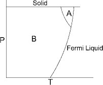
Figure 1: Pressure (P) - Temperature (T) Phase Diagram of ${}^{3}\text{He}$

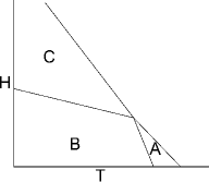
Figure 2: Magnetic Field (H) - Temperature (T) Phase Diagram of $\text{UPt}_{3}$ with B field $\perp$ z axis

Material	Fluctuations	Reps	Order Parameter	A	B
$\text{UPt}_{3}$	AFM	E	$k_{x}k_{z},k_{y}k_{z}$	(1,0)	(1,$i\delta$)
$\text{PrOs}_{4}\text{Sb}_{12}$	AFQ	E	$2k_{z}^{2}-k_{x}^{2}-k_{y},k_{x}^{2}-k_{y}^{2}$	$\times$	$\times$
		T	$k_{y}k_{z},k_{x}k_{z},k_{x}k_{y}$	(1,0,0)	$(1,i\delta,0)$ or $(1,0,i\delta)$
				(1,1,1)	$(1,1+i\delta\cos\theta,1+i\delta\sin\theta)$
$\text{U}_{1-x}\text{Th}_{x}\text{Be}_{13}$	AFM	E	$2k_{z}^{2}-k_{x}^{2}-k_{y},k_{x}^{2}-k_{y}^{2}$	(1,0)	$(1+i\delta,0)^{*}$ or $(1,i\delta)^{*}$
				(0,1)	$(0,1+i\delta)^{*}$ or $(i\delta,1)^{*}$
		T	$k_{y}k_{z},k_{x}k_{z},k_{x}k_{y}$	(1,0,0)	$(1+i\delta,0,0)^{*}$ or $(0,1+i\delta,0)$

Table 1: Table summarizing our results. The fluctuations column shows the fluctuations responsible for spin fluctuation feedback effect, whose Q vector dependence can be found in the text. The reps label the irreducible representation (reps) of the order parameter. The order parameter gives a representative basis function of the superconducting order parameter and displays the symmetry properties of it’s components. The A column is the time-reversal symmetric state, where each state is multiplied by an overall $\eta_{0}$ magnitude. The B state is the time-reversal symmetry-breaking B state grown out the A state, where the “or” separates different B reps, and we only write one state for each rep, the other degenerate states are in the text and appendix. Here $\delta$ represents a small number, which grows positively from 0 at the second transition. The $()^{*}$ is for A–B transitions which are Kerr inactive. The $\times$ represents that this channel is ruled out.

I ${}^{3}\text{He}$

${}^{3}\text{He}$ is a strongly correlated Landau-Fermi liquid, whose quasiparticle excitations pair to form a spin-triplet p-wave superfluid Leggett (1975); Vollhardt and Wölfle (2013). The gap function is $\Delta$(k) = $i(d_{i}(\textbf{k})\sigma_{i})\sigma_{y}$, with $d_{i}=d_{i\alpha}\hat{\mathbf{k}}_{\alpha}$, in this manuscript we use the Einstein summation convention. The order parameter $d_{i\alpha}$ is a 3 $\times$ 3 matrix with complex entries, where $i$ is the spin index and $\alpha$ is the orbital index and both run over $x$, $y$ and $z$. By comparing to experiments, the ${}^{3}\text{He}$-A phase was identified with the Anderson-Brinkman-Morel (ABM) state with $d_{xx}=\frac{\Delta}{\sqrt{2}},d_{xy}=i\frac{\Delta}{\sqrt{2}}$ and all other $d_{ij}=0$, while B state was associated with Balian-Wethamer (BW) which has $d_{ij}=\frac{\Delta}{\sqrt{3}}\delta_{i,j}$ Vollhardt and Wölfle (2013); Leggett (1975). Weak coupling theory showed that the BW state is stable for all temperatures Balian and Werthamer (1963), implying that a strong coupling approach was needed to explain the existence of the high temperature high pressure A phase. Anderson-Brinkman Anderson and Brinkman (1973) used spin fluctuation feedback effect to stabilize the A phase, which relied on the pairing glue in ${}^{3}\text{He}$ being paramagnetic fluctuations. This implies that the formation of the superfluid alters the pairing interaction, where the type of modification depends on which state is formed Leggett (1975). Thus the A state can be stabilized despite being unstable under weak coupling theory. The A–B transition in this case is first order as the B state is not a subgroup of the A state.

Here spin fluctuation feedback effect shall be recaptured in a phenomenological manner, by coupling the superfluid order parameter to paramagnetic fluctuations, and calculating the resulting change to the bare free energy. The bare free energy density of superfluid ${}^{3}\text{He}$ is given as

$$\beta f_{sf}=\alpha d_{i\alpha}d^{*}_{i\alpha}+\beta_{1}d_{i\alpha}d_{i\alpha}d^{*}_{j\beta}d^{*}_{j\beta}+\beta_{2}d_{i\alpha}d_{j\alpha}d^{*}_{i\beta}d^{*}_{j\beta}+\beta_{3}d_{j\alpha}d_{j\beta}d^{*}_{i\alpha}d^{*}_{i\beta}+\beta_{4}d_{i\alpha}d^{*}_{i\alpha}d_{j\beta}d^{*}_{j\beta}+\beta_{5}d^{*}_{i\alpha}d_{j\alpha}d_{i\beta}d^{*}_{j\beta}$$ (1)

To this we add the coupling of superfluidity and magnetic fluctuations, which is constructed to be invariant under independent rotations in orbital and spin space. The free energy density is given as

$$\beta f_{sf-m}=A_{1}m_{i}m_{i}+K_{1}m_{i}m_{i}d_{j\alpha}d^{*}_{j\alpha}+K_{2}m_{i}m_{j}d_{i\alpha}d^{*}_{j\alpha}+K_{3}im_{i}(\epsilon_{ijk}d_{j}d_{k}^{*})+B(\nabla_{i}m_{j})^{2},$$ (2)

where $m_{i}$ is the magnetic order parameter associated with spin fluctuations. The $K$’s are the couplings between the spin fluctuations and the superfluid order parameter, and the B term is the spatial variation (i.e. q dependence) of the spin order. We assume $A_{1}$ is parametrically small and positive (i.e. $A_{1}\rightarrow 0$) to indicate that we have large fluctuations. We have the following Hamiltonian

$$\beta\mathcal{H}=\beta\mathcal{H}_{0}+\mathcal{K}=\int d^{3}x\left[A_{1}m_{j}^{2}+B(\nabla_{i}m_{j})^{2}\right]+\int d^{3}x\left[K_{1}(m_{i}^{2})(d_{j\alpha}d^{*}_{j\alpha})+\right.\left.K_{2}m_{i}m_{j}d_{i\alpha}d^{*}_{j\alpha}+K_{3}im_{i}(\epsilon_{ijk}d_{j\alpha}d_{k\alpha}^{*})\right],$$ (3)

here $\beta\mathcal{H}_{0}$ is the Guassian theory for spin fluctuations, while $\mathcal{K}$ is the coupling between superfluid order and the spin order fluctuations. After Fourier transforming we get the following

$$\beta\mathcal{H}=\int\frac{d^{3}\textbf{q}}{(2\pi)^{3}}\left(A_{1}+Bq^{2}\right)\absolutevalue{\tilde{m}(q)}^{2}+\mathcal{K},$$ (4)

The coupling between superfluidity and magnetic fluctuations in Fourier space is

$$\mathcal{K} =\int\frac{d^{3}\mathbf{q}_{1}d^{3}\mathbf{q}_{2}d^{3}\mathbf{q}_{3}d^{3}\mathbf{q}_{4}}{(2\pi^{3})^{4}}(2\pi)^{3}\delta^{3}(\mathbf{q_{1}}+\mathbf{q_{2}}+\mathbf{q_{3}}+\mathbf{q_{4}})\left[K_{1}\tilde{m}_{i}(\mathbf{q_{1}})\tilde{m}_{i}(\mathbf{q_{2}})\tilde{d}_{j\alpha}(\mathbf{q_{3}})\tilde{d}_{j\alpha}^{*}(\mathbf{q_{4}})\right.$$

$$+K_{2}\left.\tilde{m}_{i}(\mathbf{q_{1}})\tilde{m}_{j}(\mathbf{q_{2}})\tilde{d}_{i\alpha}(\mathbf{q_{3}})\tilde{d}_{j\alpha}^{*}(\mathbf{q_{4}})\right]+K_{3}\int\frac{d^{3}\mathbf{q}_{1}d^{3}\mathbf{q}_{2}d^{3}\mathbf{q}_{3}d^{3}\mathbf{q}_{4}}{(2\pi^{3})^{3}}(2\pi)^{3}\delta^{3}(\mathbf{q_{1}}+\mathbf{q_{2}}+\mathbf{q_{3}})i\tilde{m}_{i}(\mathbf{q_{1}})\epsilon_{ijk}\tilde{d}_{j\alpha}(\mathbf{q_{2}})\tilde{d}_{k\alpha}^{*}(\mathbf{q_{3}})$$ (5)

Near the superfluid transitions, the coupling $\mathcal{K}$ can be treated perurbatively around the Gaussian theory of the magnetic fluctuations (i.e. $\beta\mathcal{H}_{0}$). This quadratic theory for spin fluctuations is valid as long as we are more than a Ginzburg temperature away from the critical temperature associated with magnetic ordering. Thus the coupling can be evaluated as

$$\beta\mathcal{H}=\beta\mathcal{H}_{0}-\ln\expectationvalue{\exp^{-\mathcal{K}}}_{m},$$ (6)

here $\expectationvalue{}_{m}$ implies that we are calculating the expectation values with respect to the Gaussian $\beta\mathcal{H}_{0}$ theory. The last expression can be expanded perturbatively around the Gaussian theory (See for e.g. Kardar (2007)) as follows

$$\ln\expectationvalue{\exp^{-\mathcal{K}}}_{m}=-\expectationvalue{\mathcal{K}}_{m}+\frac{1}{2}\left(\expectationvalue{\mathcal{K}^{2}}_{m}-\expectationvalue{\mathcal{K}}^{2}_{m}\right)+...$$ (7)

We keep upto only the $2^{nd}$ order in $\mathcal{K}$, as this will introduce corrections of $\order{d^{4}}$ to the superfluid free energy density, which will be responsible for stabilizing the A state. The first term $\expectationvalue{\mathcal{K}}_{m}$ can be evaluated and will introduce a correction to quadratic term in the superfluid Hamiltonian

$$-\expectationvalue{\mathcal{K}}_{m}= -\frac{\left(3K_{1}+K_{2}\right)}{2}\int\frac{d^{3}\mathbf{q}_{1}d^{3}\mathbf{q}_{2}d^{3}\mathbf{q}_{3}d^{3}\mathbf{q}_{4}}{(2\pi)^{12}}(2\pi)^{3}\delta^{3}(\mathbf{q_{1}}+\mathbf{q_{2}}+\mathbf{q_{3}}+\mathbf{q_{4}})\frac{(2\pi)^{3}\delta^{3}(\mathbf{q_{1}}+\mathbf{q_{2}})}{A_{1}+Bq_{1}^{2}}\tilde{d}_{i\alpha}(\mathbf{q_{3}})\tilde{d}^{*}_{i\alpha}(\mathbf{q_{4}}).$$

$$= -\frac{\left(3K_{1}+K_{2}\right)}{2}\int\frac{d^{3}\mathbf{q}_{3}}{(2\pi)^{3}}\tilde{d}_{i\alpha}(\mathbf{q_{3}})\tilde{d}^{*}_{i\alpha}(\mathbf{-q_{3}})\int\frac{d^{3}\mathbf{k}}{(2\pi)^{3}}\frac{1}{A_{1}+Bk^{2}},$$ (8)

Performing an inverse Fourier transformation we obtain the following correction to the bare superfluid free energy density

$$\beta f_{eff} =\left(\alpha+\frac{\left(3K_{1}+K_{2}\right)(2\pi)^{3}}{2\Lambda^{3}}\int^{\Lambda^{3}}\frac{d^{3}\mathbf{k}}{(2\pi)^{3}}\frac{1}{A_{1}+Bk^{2}}\right)d_{i\alpha}d^{*}_{i\alpha}+\beta_{1}d_{i\alpha}d_{i\alpha}d^{*}_{j\beta}d^{*}_{j\beta}+\beta_{2}d_{i\alpha}d_{j\alpha}d^{*}_{i\beta}d^{*}_{j\beta}$$

$$+\beta_{3}d_{j\alpha}d_{j\beta}d^{*}_{i\alpha}d^{*}_{i\beta}+\beta_{4}d_{i\alpha}d^{*}_{i\alpha}d_{j\beta}d^{*}_{j\beta}+\beta_{5}d^{*}_{i\alpha}d_{j\alpha}d_{i\beta}d^{*}_{j\beta},$$ (9)

where $\Lambda^{3}$ is a cutoff wavelength. We see that first order correction from spin fluctuation feedback effect has changed the bare $T_{c}$. The coefficient of the quadratic term is the inverse susceptibility i.e. $\chi^{-1}=A_{1}+Bq^{2}+\frac{\left(3K_{1}+K_{2}\right)(2\pi)^{3}}{\Lambda^{3}}\int^{\Lambda^{3}}\frac{d^{3}\mathbf{k}}{(2\pi)^{3}}\frac{1}{A_{1}+Bk^{2}}$. Next we calculate the crucial second order $\frac{1}{2}\left(\expectationvalue{\mathcal{K}^{2}}_{m}-\expectationvalue{\mathcal{K}}^{2}_{m}\right)$ correction which will change the coefficient of the quartic terms in the bare free energy density. We follows the exact same process as outlined above and after inverse Fourier transforming we get the following free energy density

$$\beta f_{eff}=\left(\alpha+\frac{\left(3K_{1}+K_{2}\right)(2\pi)^{3}}{2\Lambda^{3}}\int^{\Lambda^{3}}\frac{d^{3}\mathbf{k}}{(2\pi)^{3}}\frac{1}{A_{1}+Bk^{2}}\right)d_{i\alpha}d^{*}_{i\alpha}+\beta_{1}d_{i\alpha}d_{i\alpha}d^{*}_{j\beta}d^{*}_{j\beta}+\beta_{2}d_{i\alpha}d_{j\alpha}d^{*}_{i\beta}d^{*}_{j\beta}$$

$$+\left(\beta_{3}-\frac{K^{2}_{2}(2\pi)^{3}}{4\Lambda^{3}}\int^{\Lambda^{3}}\frac{d^{3}\mathbf{k}}{(2\pi)^{3}}\frac{1}{(A_{1}+Bk^{2})^{2}}\right)d_{j\alpha}d_{j\beta}d^{*}_{i\alpha}d^{*}_{i\beta}+\left(\beta_{5}-\frac{K^{2}_{2}(2\pi)^{3}}{4\Lambda^{3}}\int^{\Lambda^{3}}\frac{d^{3}\mathbf{k}}{(2\pi)^{3}}\frac{1}{(A_{1}+Bk^{2})^{2}}\right)d^{*}_{i\alpha}d_{j\alpha}d_{i\beta}d^{*}_{j\beta}$$

$$+\left(\beta_{4}-\frac{\left(K^{2}_{2}+6K_{1}^{2}+4K_{1}K_{2}\right)(2\pi)^{3}}{2\Lambda^{3}}\int^{\Lambda^{3}}\frac{d^{3}\mathbf{k}}{(2\pi)^{3}}\frac{1}{(A_{1}+Bk^{2})^{2}}\right)d_{i\alpha}d^{*}_{i\alpha}d_{j\beta}d^{*}_{j\beta}$$

$$-\frac{K^{2}_{3}(2\pi)^{3}}{2\Lambda^{3}}\int^{\Lambda^{3}}\frac{d^{3}\mathbf{k}}{(2\pi)^{3}}\frac{1}{(A_{1}+Bk^{2})}\left(i\vec{d}\times\vec{d}^{*}\right)^{2},$$ (10)

Let us now consider a simpler situation, where we ignore the cost of spatial variation in the spin fluctuation order parameter (i.e. $B$ = 0). Thus we have the following coupling

$$\beta f_{sf-m}=A_{1}m_{i}m_{i}+K_{1}m_{i}m_{i}d_{j\alpha}d^{*}_{j\alpha}+K_{2}m_{i}m_{j}d_{i\alpha}d^{*}_{j\alpha}+K_{3}im_{i}(\epsilon_{ijk}d_{j\alpha}d_{k\alpha}^{*}),$$ (11)

The magnetic partition function is given as

$$\mathcal{Z}_{m}=\int Dm_{i}e^{-\beta\mathcal{H}}=\int Dm_{i}e^{-\int d^{3}xf_{sf-m}}=\int Dm_{i}e^{-\int d^{3}xA_{ij}m_{i}m_{j}},$$ (12)

where $A_{ij}$ contains couplings between magnetic and superconducting orders, and give corrections the bare superconducting free energy density. Integrating out the quadratic (Gaussian) magnetic fluctuations, gives an effective free energy density

$$\beta f_{eff} =\left(\alpha+\frac{3K_{1}}{2A_{1}}+\frac{K_{2}}{2A_{1}}\right)d_{i\alpha}d^{*}_{i\alpha}+\beta_{1}d_{i\alpha}d_{i\alpha}d^{*}_{j\beta}d^{*}_{j\beta}+\beta_{2}d_{i\alpha}d_{j\alpha}d^{*}_{i\beta}d^{*}_{j\beta}+\left(\beta_{3}-\frac{K_{2}^{2}}{4A_{1}^{2}}\right)d_{j\alpha}d_{j\beta}d^{*}_{i\alpha}d^{*}_{i\beta}$$

$$+\left(\beta_{4}-\frac{K_{2}^{2}+6K_{1}^{2}+4K_{2}K_{1}}{2A_{1}^{2}}\right)d_{i\alpha}d^{*}_{i\alpha}d_{j\beta}d^{*}_{j\beta}+\left(\beta_{5}-\frac{K_{2}^{2}}{4A_{1}^{2}}\right)d^{*}_{i\alpha}d_{j\alpha}d_{i\beta}d^{*}_{j\beta}-\frac{K_{3}^{2}}{2A_{1}}\left(i\vec{d}\times\vec{d}^{*}\right)^{2},$$ (13)

Now if we compare Eq. (I) and Eq. (I), we note that even though the corrections introduced to the free energy density have different forms in both cases, the sign of the correction introduced is the same, i.e. in both cases the spin fluctuation feedback effect leads to corrections which can stabilize a different state than the state preferred by the weak coupling theory. Subsequently, for clarity, we use the simplified result since it yields qualitatively the same results.

The $\beta_{i}$ quartic terms in Eq. (I) are associated with the free energy density without coupling to fluctuations, here assumed to be derived from weak-coupling theory and the quartic terms with the $K$’s originate from spin fluctuation feedback effect.

For large paramagnetic fluctuations, i.e. a small but positive $A_{1}$, the terms that dominate are those that are proportional to $A_{1}^{-2}$ and we ignore terms of order $A_{1}^{-1}$ (for e.g. couplings of the form $m^{2}d^{4}$ ). The $K_{3}$ term in Eq. (I) shows that paramagnetic fluctuations can favor non-unitary states Gorkov (1987); Mineev and Samokhin (1999); Choi and Muzikar (1989); Walker and Samokhin (2002), but will neglected here due to it’s weaker $A_{1}^{-1}$ dependence.

Weak coupling theory gives $\beta_{2}=\beta_{3}=\beta_{4}=-\beta_{5}=2\beta_{1}=\frac{6}{5}s$, where $s$ is a positive valued constant Leggett (1975); Vollhardt and Wölfle (2013). When the spin fluctuation feedback effect is turned off (i.e. $K_{i}=0$), the BW state is energetically favorable with $f_{eff}=\frac{5}{3}s$, while the A state has a slightly larger free energy density of $f_{eff}=2s$. The spin fluctuation feedback effect coupling lowers the energy of the A state by $K_{2}^{2}/3A_{1}^{2}$ compared to the B state and thus for large fluctuations (i.e. $K_{2}^{2}/3A_{1}^{2}>\frac{1}{3}s$) can stabilize the A state. Kuroda (1975)

The A–B transition stems from the different temperature dependence of the weak coupling quartic terms versus the spin fluctuation feedback effect corrections to the quartic terms. Quartic (i.e. $\beta$) terms originating from weak coupling theory generically have a $\frac{1}{\text{T}^{2}}$ dependence Mineev and Samokhin (1999), while microscopic calculations show that quartic terms originating from the spin fluctuation feedback effect have a $\frac{1}{\text{T}}$ dependence Brinkman et al. (1974); Leggett (1975); Kuroda (1975). These calculations assumed quadratic, Gaussian spin fluctuations and imply that at high temperatures, strong fluctuations may stabilize the A phase, while at lower temperature the weak coupling terms will dominate and the system will undergo a first order transition into the state preferred by weak coupling theory i.e. the B phase. Recent calculations done for twisted bilayer graphene Kozii et al. (2019), show that the same temperature dependence of the quartic terms is seen for both spin density and charge density wave fluctuations, again considering Gaussian fluctuations. This suggests that the weak-coupling quartic terms and spin-fluctuation corrections to these terms generically have a $1/T$ and $1/T^{2}$ temperature dependence respectively. We will assume this to be the case in the correlated fermion materials considered below.

II $\text{UPt}_{3}$

$\text{UPt}_{3}$ is a hexagonal crystal with $D_{6h}$ point group symmetry and has two distinct phases under zero field, a high temperature A phase and a low temperature B phase Stewart et al. (1984); Joynt and Taillefer (2002). However, unlike ${}^{3}\text{He}$, the A phase is time-reversal symmetric while the B phase is time-reversal symmetry-breaking as seen in muon spin relaxation ($\mu$SR) and polar Kerr measurements Luke et al. (1993); Schemm et al. (2014). $\text{UPt}_{3}$ has four 2D (reps) labeled $E_{1u/g}$ and $E_{2u/g}$, where the order parameter transforms like $\eta_{1}\sim k_{x}k_{z}$, $\eta_{2}\sim k_{y}k_{z}$ and $\eta_{1}\sim k_{x}^{2}-k_{y}^{2}$, $\eta_{2}\sim 2k_{x}k_{y}$ respectively. The free energy density is the same for all the $E$ reps and is given as Sigrist and Ueda (1991).

$$\beta f_{sc}=\alpha\left(\absolutevalue{\eta_{1}}^{2}+\absolutevalue{\eta_{1}}^{2}\right)+\beta_{1}\left(\absolutevalue{\eta_{1}}^{2}+\absolutevalue{\eta_{1}}^{2}\right)^{2}+\beta_{2}\absolutevalue{\eta_{1}^{2}+\eta_{2}^{2}}^{2}$$ (14)

The coefficient of $\absolutevalue{\eta_{i}^{2}}^{2}$ determines the behavior below $T_{c}$, with $\beta_{2}>0$ favoring the time-reversal symmetry-breaking $(1,i)$ state, and $\beta_{2}<0$ stabilizing the time-reversal symmetric $(1,0)$ state. To explain the existence of multiple phases, the currently accepted model involves coupling superconductivity to antiferromagnetic order Machida et al. (1989); Hess et al. (1989). This splits the $T_{c}$ between $\eta_{1}$ and $\eta_{2}$ and allows for two transitions.

However, recent experiments raise questions over the existence of true antiferromagnetic order near the two closely spaced superconducting transitions. The Bragg peaks in inelastic nuetron scattering are not resolution limited near the superconducting transitions of $T_{cA}=530mK$ and $T_{cB}=480mK$ Joynt and Taillefer (2002); Koike et al. (1998, 1999), in addition to the absence of signatures of a magnetic transition in specific heat, magnetization and NMR Knight shift experiments around this temperature. The peaks start narrowing only below 50mK and become resolution limited at 20 mK Koike et al. (1998, 1999), which seems consistent with anomalies seen in specific heat Schuberth et al. (1992); Schuberth (1996), thermal expansion Sawada et al. (1996) and magnetization measurements Schöttl et al. (1999) seen near 20mK. Interestingly, NMR experiments show an anomaly at 50mK which is associated with the fluctuations slowing down, though there is no sign of static order down till 15mK Kitaoka et al. (2000); Van Dijk et al. (2002).

This has lead to the current interpretation that these experiments imply the presence of antiferromagnetic fluctuations Gannon et al. (2017), instead of antiferromagnetic order, and we suggest that a generalized spin fluctuation feedback effect then stabilizes a time-reversal symmetric A state.

Our theory is a Ginzburg-Landau theory and is valid near the A–B transition and cannot be extended deep into the B state. However, the use of spin fluctuation feedback effect fluctuations to generate two closely spaced transitions should be valid near the superconducting transitions (i.e. $T_{c}$ $\sim$ 500mK). We note that the Ginzburg temperature for magnetic transitions is generically of the order $1-10^{-2}$mK of the magnetic transition temperature ( which for $\text{UPt}_{3}$ is $T_{cm}\sim 50mK$). Consequently, the superconducting A–B transitions will be insensitive to critical phenomena stemming from the possible ultra low temperature magnetic ordering. Additionally, there are no signatures of quantum critical effects in this material and the other materials considered in this manuscript. Hence arguments similar to those developed for superfluid ${}^{3}\text{He}$ can be used to explain two transitions in $\text{UPt}_{3}$, and it suffices to consider a Gaussian theory of spin fluctuations.

We shall proceed analogously to ${}^{3}\text{He}$, and assume that the B time-reversal symmetry-breaking state is favored by the weak coupling theory, while strong fluctuations can stabilize a time-reversal symmetric A phase. The fluctuations are characterized by wave vectors Q₁=$\frac{1}{2}$ a^∗, Q₂=$\frac{1}{2}$(b^∗-a^∗), Q₃= -$\frac{1}{2}$b^∗ Aeppli et al. (1988); Koike et al. (1998) which are associated with the magnetic order parameters $m_{1}$, $m_{2}$ and $m_{3}$ respectively. The coupling of superconductivity to the magnetic fluctuations is constructed to be invariant under $D_{6h}\times U(1)\times\mathscr{T}$, where $\mathscr{T}$ is time-reversal symmetry and is expressed as Machida et al. (1989)

$$\beta f_{sc-m}=A_{1}m_{i}^{2}+K_{1}(m_{i}^{2})(\eta_{j}\eta_{j}^{*})+K_{2}\left[(2m_{1}^{2}-m_{2}^{2}-m_{3}^{2})(\absolutevalue{\eta_{1}}^{2}-\absolutevalue{\eta_{2}}^{2})+\sqrt{3}(m_{3}^{2}-m_{2}^{2})(\eta_{1}\eta_{2}^{*}+\eta_{2}\eta_{1}^{*})\right].$$ (15)

Integrating out the fluctuations as before gives the following free energy density:

$$\left(\alpha+\frac{3}{2}\frac{K_{1}}{A_{1}}\right)\left(\absolutevalue{\eta_{1}}^{2}+\absolutevalue{\eta_{1}}^{2}\right)+\left(\beta_{1}-\frac{3}{4}\frac{K_{1}^{2}}{A_{1}^{2}}\right)\left(\absolutevalue{\eta_{1}}^{2}+\absolutevalue{\eta_{1}}^{2}\right)^{2}+\left(\beta_{2}-\frac{6}{4}\frac{K_{2}^{2}}{A_{1}^{2}}\right)\absolutevalue{\eta_{1}^{2}+\eta_{2}^{2}}^{2}.$$ (16)

We see that the terms originating from the generalized spin fluctuation feedback effect have introduced negative valued corrections to the quartic terms, which most importantly changes the $\absolutevalue{\eta_{i}^{2}}^{2}$ coefficient. Thus for large fluctuations, these spin fluctuation feedback effect terms can stabilize the A state, instead of the time-reversal symmetry-breaking B by making this coefficient negative.

This also interestingly implies that two transitions will occur only if the B state is a broken time-reversal symmetry state. In particular, if the B state was time-reversal symmetric then the spin fluctuation feedback effect terms would simply further stabilize the time-reversal symmetric nematic state.

As argued earlier, the quartic terms that stem from weak-coupling theory should increase more strongly as temperature is decreased than the quartic terms which arise from the generalized spin fluctuation feedback effect. This allows the coefficient of the $\absolutevalue{\eta_{1}^{2}+\eta_{2}^{2}}^{2}$ to change sign as temperature is decreased, so that a transition into the a broken time-reversal symmetry state is possible. We discuss this in more detail below.

II.1 Effective theory for A–B transitions

A complete phenomenological description of a second phase transition within a single multi-dimensional rep requires a free energy density that is at least eighth order in the order parameter Gufan (1995); Toledano and Toledano (1987). For this reason, we consider a simpler approach and model the A–B transition as an effective phenomenological theory in which we start with $(1,0)$ state for $\text{UPt}_{3}$ and allow the B state to continuously grow out of this i.e. $(1+\tilde{\eta}_{1i},0+\tilde{\eta}_{2i})$, where $\tilde{\eta}_{i}$ is small near the transition. Time-reversal symmetry allows us to classify the order parameter $\tilde{\eta}_{i}$ for the A–B transition into a real part $\tilde{\eta}_{R}$ which is invariant under $\mathscr{T}$, and an imaginary part $\tilde{\eta}_{I}$ which changes sign under $\mathscr{T}$, with the following transformation properties.

$$\tilde{\eta}_{R}\overset{\mathcal{T}}{\rightarrow}\tilde{\eta}_{R}\hskip 35.00005pt\tilde{\eta}_{I}\overset{\mathcal{T}}{\rightarrow}-\tilde{\eta}_{I}.$$ (17)

The condition that the second transition is observed to break time-reversal symmetry, allows us to consider only the imaginary order parameter. The $(1,0)$ state has $D_{2}(C_{2})\times\mathscr{T}$ and $D_{2}\times\mathscr{T}$ Gorkov (1987) symmetry for the $E_{1u/g}$ and $E_{2u/g}$ reps respectively. The order parameter $\tilde{\eta}_{1I}$ belongs to the $A_{1}$ rep of $D_{2}$, while $\tilde{\eta}_{2I}$ belongs to the $B_{1}$ rep. Hence our mechanism only allows these two possible symmetries for the $B$ phase.

II.2 Constraints from polar Kerr effect

The observation of a polar Kerr signal for the A–B transition Schemm et al. (2014) further constrains the possible order parameters. In particular, polar Kerr experiments shows that signal can be trained with an applied magnetic field Schemm et al. (2014). This implies that the only viable order parameters are those which belong to the same representation as a component of the magnetic field ($H_{x}$, $H_{y}$, $H_{z}$). This follows because a Kerr signal that can be trained in field is only possible if the superconducting order parameter couples linearly to the applied field. These order parameters shall be referred to as Kerr active (in the literature, this is sometimes labeled as belonging to a ferromagnetic class Volovik and Gor’kov (1985)). This rules out the $A_{1}$ order parameter since it is Kerr inactive. The $\tilde{\eta}_{2I}$ order parameter has $H_{z}$ symmetry, which is consistent with the direction of the training field applied along the c-axis in the experiment. Thus the A–B transition can be modeled by the effective order parameter $\tilde{\eta}_{2I}$ with the following free energy $\beta f_{A\rightarrow B}=\alpha_{1I}\tilde{\eta}_{2I}^{2}+\beta_{1I}\tilde{\eta}_{2I}^{4}$. We shall use this approach subsequently to constrain the possible symmetries of the order parameters.

III $\text{PrOs}_{4}\text{Sb}_{12}$

$\text{PrOs}_{4}\text{Sb}_{12}$ (POS) is a Pr based tetrahedral correlated fermion skutterudite superconductor with a $T_{h}$ point group, and like $\text{UPt}_{3}$ has two distinct phases Vollmer et al. (2003). Polar Kerr and $\mu$SR measurements show a time-reversal symmetry-breaking B phase Aoki et al. (2003); Levenson-Falk et al. (2018), while the A phase is time-reversal symmetric. POS has been studied by phenomenological methods Sergienko and Curnoe (2004), however there is no satisfactory mechanism for the double transition. Inelastic nuetron scattering experiments indicate the presence of antiferro-quadrupolar fluctuations with a Q = (1, 0, 0) Kaneko et al. (2007); Kuwahara et al. (2005), which is a single Q order, invariant under the point group operations. The order parameter of these antiferro-quadrupolar fluctuations is 3D with components that transform as $m_{1}\sim k_{y}k_{z}$, $m_{2}\sim k_{x}k_{z}$ and $m_{3}\sim k_{x}k_{y}$ Shiina (2004); Shiina and Aoki (2004). The antiferro-quadrupolar fluctuations can stabilize a time-reversal symmetric A phase for both the $E$ and $T$ reps as shown below.

For the $E$ reps, where the order parameter transforms as $\eta_{1}\sim 2k_{z}^{2}-k_{x}^{2}-k_{y}^{2}$, $\eta_{2}\sim k_{x}^{2}-k_{y}^{2}$, the coupling is

$$\beta f_{sc-m} =A_{1}(m_{i}^{2})+K_{1}(m_{j}^{2})(\eta_{j}\eta_{j}^{*})+K_{2}\left[(2m_{3}^{2}-m_{1}^{2}-m_{2}^{2})(\absolutevalue{\eta_{1}}^{2}-\absolutevalue{\eta_{2}}^{2})-\sqrt{3}(m_{1}^{2}-m_{2}^{2})(\eta_{1}\eta_{2}^{*}+\eta_{2}\eta_{1}^{*})\right]$$

$$+K_{3}\left[\sqrt{3}(m_{1}^{2}-m_{2}^{2})(\absolutevalue{\eta_{1}}^{2}-\absolutevalue{\eta_{2}}^{2})+(\eta_{1}\eta_{2}^{*}+\eta_{2}\eta_{1}^{*})(2m_{3}^{2}-m_{1}^{2}-m_{2}^{2})\right].$$ (18)

As noted in $\text{UPt}_{3}$, we shall consider the simple case of $B(\nabla\vec{m})^{2}=0$. Integrating out the antiferro-quadrupolar fluctuations, we obtain the effective free energy density

$$\beta f_{eff}=\left(\alpha+\frac{3K_{1}}{2A_{1}}\right)(\eta_{j}\eta_{j}^{*})+\left(\beta_{1}-\frac{3K_{1}^{2}}{4A_{1}^{2}}-\frac{3K_{2}^{2}}{2A_{1}^{2}}-\frac{3K_{3}^{2}}{2A_{1}^{2}}\right)\left(\eta_{j}\eta_{j}^{*}\right)^{2}+\left(\beta_{2}-\frac{3K_{2}^{2}}{2A_{1}^{2}}-\frac{3K_{3}^{2}}{2A_{1}^{2}}\right)(\eta_{1}\eta_{2}^{*}-\eta_{2}\eta_{1}^{*})^{2}.$$ (19)

This generalized spin fluctuation feedback effect may again stabilize a time-reversal symmetric A state $(\phi_{1},\phi_{2})$ with $D_{2}\times\mathscr{T}$ symmetry Sergienko and Curnoe (2004); Mukherjee and Agterberg (2006), instead of the time-reversal symmetry-breaking B phase $(1,i)$ with $T(D_{2})$ symmetry by changing the sign of the $(\eta_{1}\eta_{2}^{*}-\eta_{2}\eta_{1}^{*})^{2}$ term from positive to negative. The A phase has the two components with the same magnitude but an arbitrary phase Sergienko and Curnoe (2004). Similar to $\text{UPt}_{3}$ two transitions are possible only when the B state is time-reversal symmetry-breaking. The A–B transition is modeled similar to $\text{UPt}_{3}$, however both $\eta_{1I/2I}$ have $A_{1}$ Kerr inactive symmetry and are ruled out due to presence of Kerr effect, thereby eliminating the 2D E reps scenario for $\text{PrOs}_{4}\text{Sb}_{12}$.Thus we can see just using these general symmetry considerations we are able to rule out a pairing scenario with this mechanism.

For the 3D $T_{g/u}$ reps, with order parameter which transforms for example as $\eta_{1}\sim k_{y}k_{z}$, $\eta_{2}\sim k_{x}k_{z}$ and $\eta_{3}\sim k_{x}k_{y}$, the coupling is

$$\beta f_{sc-m} =A_{1}\left(m_{i}^{2}\right)+K_{1}(\eta_{j}\eta_{j}^{*})\left(m_{j}^{2}\right)+K_{2}\left[3\left(\absolutevalue{\eta_{2}}^{2}-\absolutevalue{\eta_{3}}^{2}\right)\left(m_{2}^{2}-m_{3}^{2}\right)+\left(2\absolutevalue{\eta_{1}}^{2}-\absolutevalue{\eta_{2}}^{2}-\absolutevalue{\eta_{3}}^{2}\right)\right.$$

$$\times\left.\left(2m_{1}^{2}-m_{2}^{2}-m_{3}^{2}\right)\right]+K_{3}\left[\left(\absolutevalue{\eta_{2}}^{2}-\absolutevalue{\eta_{1}}^{2}\right)\left(2m_{1}^{2}-m_{2}^{2}-m_{3}^{2}\right)-\left(2\absolutevalue{\eta_{1}}^{2}-\absolutevalue{\eta_{2}}^{2}-\absolutevalue{\eta_{3}}^{2}\right)\left(m_{2}^{2}-m_{3}^{2}\right)\right]$$

$$+K_{4}\left[\left(\eta_{2}\eta_{3}^{*}+\eta_{2}^{*}\eta_{3}\right)m_{2}m_{3}+\left(\eta_{3}\eta_{1}^{*}+\eta_{3}^{*}\eta_{1}\right)m_{3}m_{1}+\left(\eta_{1}\eta_{2}^{*}+\eta_{1}^{*}\eta_{2}\right)m_{1}m_{2}\right].$$ (20)

Integrating out the Gaussian antiferro-quadrupolar fluctuations gives the following effective free energy density:

$$\beta f_{eff} =\left(\alpha+3\frac{K_{1}}{A_{1}}\right)(\eta_{j}\eta_{j}^{*})+\left(\beta_{1}-\frac{6K_{1}^{2}}{A_{1}^{2}}+\frac{6K_{2}^{2}}{A_{1}^{2}}+\frac{2K_{3}^{2}}{A_{1}^{2}}-\frac{K_{4}^{2}}{4A_{1}^{2}}\right)\left(\eta_{j}\eta_{j}^{*}\right)^{2}+\left(\beta_{2}-\frac{K_{4}^{2}}{4A_{1}^{2}}\right)\absolutevalue{\eta_{i}^{2}}^{2}$$

$$+\left(\beta_{3}-\frac{18K_{2}^{2}}{A_{1}^{2}}-\frac{6K_{3}^{2}}{A_{1}^{2}}+\frac{K_{4}^{2}}{2A_{1}^{2}}\right)\left(\absolutevalue{\eta_{1}}^{4}+\absolutevalue{\eta_{2}}^{4}+\absolutevalue{\eta_{3}}^{4}\right).$$ (21)

Again the generalized spin fluctuation feedback effect has changed the coefficient of the bare free energy density and hence allows for the possibility of a time-reversal symmetric A state. Interestingly, here we may have two transition even if the A state is time-reversal symmetry-breaking, due the indeterminant sign of the correction to the $\beta_{3}$ coefficient. However since this does not agree with the experimental identification of the B state having broken time-reversal symmetry, we don’t consider this possibility. This rep has two states which are time-reversal symmetric, the $(1,0,0)$ state with $D_{2}(C_{2})\times\mathscr{T}$ symmetry and the $(1,1,1)$ state with $C_{3}\times\mathscr{T}$ symmetry. Both of these allow for a transition to a time-reversal symmetry-breaking B state which is Kerr active and hence provide two viable channels for the transition. The physics of this is similar to the 2D rep case for $\text{UPt}_{3}$ and is worked out in the appendix, the results of which are collected in Table 1. It would be of interest to carry out Kerr measurements Levenson-Falk et al. (2018) under different directions of training field to further constrain the possible pairing channels.

IV $\text{U}_{1-x}\text{Th}_{x}\text{Be}_{13}$

$\text{U}_{1-x}\text{Th}_{x}\text{Be}_{13}$ is a cubic material with an $\text{O}_{h}$ point group, which also has two transitions Heffner et al. (1990); Zieve et al. (2004), but only for a doping range of 2 % $<$ x $<$ 4 %. The B phase is again a time-reversal symmetry-breaking state Heffner et al. (1990). Antiferromagnetic fluctuations are seen in inelastic nuetron scattering with a wave vector of Q₃ = (1/2, 1/2, 0) Hiess et al. (2002). We consider both the $E$ and $T$ reps and model the system with O_h symmetry, having antiferromagnetic fluctuations with wave vector Q₃. The star of Q₃ gives two additional wave vectors Q₂ = (1/2, 0, 1/2) and Q₁ = (0, 1/2, 1/2), each of which correspond to a 1D order parameter $m_{1}$, $m_{2}$, $m_{3}$. Here $\eta_{1}$ and $\eta_{2}$ transform exactly as $E$ reps of $\text{PrOs}_{4}\text{Sb}_{12}$. The coupling is

$$\beta f_{sc-m} =A_{1}(m_{i}^{2})+K_{1}(m_{i}^{2})(\eta_{j}\eta_{j}^{*})+K_{2}\left[(2m_{3}^{2}-m_{1}^{2}-m_{2}^{2})(\absolutevalue{\eta_{1}}^{2}-\absolutevalue{\eta_{2}}^{2})-\sqrt{3}(m_{1}^{2}-m_{2}^{2})(\eta_{1}\eta_{2}^{*}+\eta_{2}\eta_{1}^{*})\right].$$ (22)

The $K_{3}$ term present in Eq. III is absent above, due to additional symmetry elements present in the $O_{h}$ as compared to $T_{h}$ point group. The correction to the free energy density from these fluctuations is

$$\beta f_{eff}=\left(\alpha+\frac{3K_{1}}{2A_{1}}\right)(\eta_{j}\eta_{j}^{*})+\left(\beta_{1}-\frac{3K_{1}^{2}}{4A_{1}^{2}}-\frac{3K_{2}^{2}}{2A_{1}^{2}}\right)\left(\eta_{j}\eta_{j}^{*}\right)^{2}+\left(\beta_{2}-\frac{3K_{2}^{2}}{2A_{1}^{2}}\right)(\eta_{1}\eta_{2}^{*}-\eta_{2}\eta_{1}^{*})^{2}.$$ (23)

There are two possible time-reversal symmetric A states. The details of the A–B effective theory follows that of $\text{UPt}_{3}$ and is in the appendix, with the possible A state being (1,0) with $D_{4}\times\mathscr{T}$ symmetry and (0,1) with $D_{4}^{(1)}(D_{2})\times\mathscr{T}$ symmetry Volovik and Gor’kov (1985). These states are Kerr inactive, and we suggest that a polar Kerr measurement be performed on this material. If a field-trainable polar Kerr signal is seen then the 2D order parameter can be ruled out.

For the 3D order parameter case, we note that, $\text{U}_{1-x}\text{Th}_{x}\text{Be}_{13}$ has four $T$ reps, one which transforms exactly like $T$ reps of $\text{PrOs}_{4}\text{Sb}_{12}$ which we call $T_{2g/u}$ and the other $T_{1g/u}$ which transforms as $\eta_{1}\sim k_{y}k_{z}(k_{y}^{2}-k_{z}^{2})$, $\eta_{1}\sim k_{z}k_{x}(k_{z}^{2}-k_{x}^{2})$ and $\eta_{3}\sim k_{x}k_{y}(k_{x}^{2}-k_{y}^{2})$. The coupling for these $T$ reps is

$$f_{sc-m}=A_{1}\left(m_{i}^{2}\right)+K_{1}\left(m_{i}^{2}\right)(\eta_{j}\eta_{j}^{*})+K_{2}\left[3\left(\absolutevalue{\eta_{2}}^{2}-\absolutevalue{\eta_{3}}^{2}\right)\left(m_{2}^{2}-m_{3}^{2}\right)+\left(2\absolutevalue{\eta_{1}}^{2}-\absolutevalue{\eta_{2}}^{2}-\absolutevalue{\eta_{3}}^{2}\right)\left(2m_{1}^{2}-m_{2}^{2}-m_{3}^{2}\right)\right].$$ (24)

The $K_{3}$ term found in Eq. III is absent because of higher $O_{h}$ symmetry compared to the $T_{h}$ symmetry, while the $K_{4}$ term is forbidden as $m_{i}m_{j}$ is not translationally invariant for this Q vector. The effective free energy density obtained is

$$\beta f_{eff}=\left(\alpha+3\frac{K_{1}}{A_{1}}\right)(\eta_{j}\eta_{j}^{*})+\left(\beta_{1}-\frac{3K_{1}^{2}}{4A_{1}^{2}}+\frac{3K_{2}^{2}}{A_{1}^{2}}\right)\left(\eta_{j}\eta_{j}^{*}\right)^{2}+\beta_{2}\absolutevalue{\eta_{j}^{2}}^{2}+\left(\beta_{3}-\frac{9K_{2}^{2}}{A_{1}^{2}}\right)\left(\absolutevalue{\eta_{1}}^{4}+\absolutevalue{\eta_{2}}^{4}+\absolutevalue{\eta_{3}}^{4}\right).$$ (25)

Interestingly, here unlike $\text{PrOs}_{4}\text{Sb}_{12}$ there is no change to $\beta_{2}$, which is a result of the $K_{4}$ coupling being absent for Eq. 25 in contrast to Eq. III. There are four possible time-reversal symmetric A state, two for each $T$ reps, i.e. (1,0,0) and (1,1,1). However due to there being no change to coefficient of the $\absolutevalue{\eta_{i}^{2}}^{2}$ term, the (1,0,0) is the only time-reversal symmetric A state which allows for a viable transition to a time-reversal symmetry-breaking B state Gorkov (1987). This state has $D_{4}(C_{4})\times\mathscr{T}$ and $D_{4}^{(2)}(D_{2})\times\mathscr{T}$ symmetry for the $T_{1}$ and $T_{2}$ reps respectively Volovik and Gor’kov (1985). The A–B transition, follows similar to $\text{UPt}_{3}$, and is modeled in the appendix. Polar Kerr measurements especially if trainable by field, may be useful as they can rule out the $E_{g/u}$ reps scenario, and can eliminate other 3D $T_{g/u}$ order parameters.

V Conclusions

In analogy to superfluid ${}^{3}\text{He}$, we have argued that a generalized spin fluctuation feedback effect can account for multiple transitions seen in correlated fermion materials. We have provided a simple phenomenological framework to capture this and show that this naturally provides a unifying mechanism for two superconducting transitions observed in $\text{UPt}_{3}$, $\text{PrOs}_{4}\text{Sb}_{12}$ and $\text{U}_{1-x}\text{Th}_{x}\text{Be}_{13}$. In addition, the use of this generalized spin fluctuation feedback effect allows us to constrain various pairing symmetries. The results of this analysis are tabulated in Table 1. In particular, we are able to rule out the 2D ($E_{g/u}$) scenario for $\text{PrOs}_{4}\text{Sb}_{12}$, while for the the 3D ($T_{g/u}$) reps of $\text{U}_{1-x}\text{Th}_{x}\text{Be}_{13}$ only one of two possible A states is allowed. Additionally, if a polar Kerr signal is observed for $\text{U}_{1-x}\text{Th}_{x}\text{Be}_{13}$, we will be able to rule out the 2D ($E_{g/u}$) for $\text{U}_{1-x}\text{Th}_{x}\text{Be}_{13}$, and place further constraints on other pairing channels.

Acknowledgments.- Adil Amin and D.F.A. acknowledge financial support through the UWM research growth initiative. We would like to thank Aharon Kapitulnik, Bill Halperin, Deep Chatterjee and Joseph O’ Halloran for useful discussions.

Appendix A Effective theory for A–B transition

$\text{PrOs}_{4}\text{Sb}_{12}$.- For the 3D $T_{1g/u}$ reps, we have two possible time-reversal symmetric A states the $(1,0,0)$ state with $D_{2}(C_{2})\times\mathscr{T}$ symmetry and the $(1,1,1)$ state with $C_{3}\times\mathscr{T}$ symmetry. Both of these allow for a transition to a time-reversal symmetry-breaking B state which is Kerr active and hence provide two viable channels for the transition. In the case of $(1+\tilde{\eta}_{1I},0+\tilde{\eta}_{2I},0+\tilde{\eta}_{3I})$, $\tilde{\eta}_{1I}$ belongs to the $A_{1}$ Kerr inactive reps and hence is not considered, while $\tilde{\eta}_{2I}$ and $\tilde{\eta}_{3I}$ belong to the Kerr active $B_{1}$ and $B_{2}$ reps respectively. The form of the free energy will look similar to the 1D A–B transition in $\text{UPt}_{3}$, and the exact transition would depend on which rep has a higher $T_{c}$. The free energy will be

$$\beta f_{A\rightarrow B}=\alpha_{I}\tilde{\eta}_{2/3I}^{2}+\beta_{I}\tilde{\eta}_{2/3I}^{4}.$$ (26)

For the $(1+\tilde{\eta}_{1I},1+\tilde{\eta}_{2I},1+\tilde{\eta}_{3I})$ state we have a 1D $A_{1}$ Kerr inactive order parameter defined as $\eta_{A}=\tilde{\eta}_{1}+\tilde{\eta}_{2}+\tilde{\eta}_{3}$ and which is ignored, and a 2D Kerr active $E$ order parameter, defined as

$$\eta_{x}=\frac{1}{\sqrt{6}}(2\tilde{\eta_{3}}-\tilde{\eta_{2}}-\tilde{\eta_{3}}),\hskip 5.0pt\eta_{y}=\frac{1}{\sqrt{2}}(\tilde{\eta_{1}}-\tilde{\eta_{2}}),$$ (27)

where $\eta_{x},\eta_{y}$ belong to the 2D Kerr active $E$ reps of $C_{3}$. The free energy for this $E$ rep is

$$\beta f^{E}_{A\rightarrow B}=\alpha_{I}\eta_{i}^{2}+\beta_{1I}\left(\eta_{i}^{2}\right)^{2}+\gamma\left(\eta_{i}^{2}\right)^{3}+\gamma_{1}\eta_{xI}^{2}(\eta_{xI}^{2}-3\eta_{yI}^{2})^{2}+\gamma_{2}\eta_{yI}^{2}(3\eta_{xI}^{2}-\eta_{yI}^{2})^{2}+\gamma_{3}\eta_{xI}\eta_{yI}(\eta_{xI}^{2}-3\eta_{yI}^{2})(3\eta_{xI}^{2}-\eta_{yI}^{2})$$ (28)

Once $\alpha_{I}$ changes sign the ground state will be $\eta$ = $\eta_{I}$($\cos\theta,\sin\theta$), where the value of $\theta$ will depend on the value of the coefficients ($\gamma_{i}$) of the 6${}^{\text{th}}$ order terms, and hence provides a viable mechanism for a transitions to a time-reversal symmetry-breaking B phase.

$\text{U}_{1-x}\text{Th}_{x}\text{Be}_{13}$.- For the 2D $E_{g/u}$ reps there are two possible time-reversal symmetric A states. We model the A–B transition as done before, with the A state being (1,0) possessing $D_{4}\times\mathscr{T}$ symmetry and (0,1) with $D_{4}^{(1)}(D_{2})\times\mathscr{T}$ symmetry Volovik and Gor’kov (1985). The B state grows as $(1+\tilde{\eta}_{1I},0+\tilde{\eta}_{2I})$, where $\tilde{\eta}_{1I}$ belongs to the $A_{1}$ and $\tilde{\eta}_{2I}$ belongs to $B_{1}$ reps of $D_{4}$, while for the $(0,1)$ state, the situation is reversed. In that case the the B state grows as $(0+\tilde{\eta}_{1I},1+\tilde{\eta}_{2I})$, with with $\tilde{\eta}_{1I}$ having $B_{1}$ symmetry and $\tilde{\eta}_{2I}$ belonging to the $A_{1}$ rep of $D_{4}$. The free energy will be the same as for the 1D order parameters

$$\beta f_{A\rightarrow B}=\alpha_{I}\tilde{\eta}_{1/2I}^{2}+\beta_{I}\tilde{\eta}_{1/2I}^{4}.$$ (29)

Interestingly due the absence of a Kerr measurement experiment, the $A_{1}$ rep is viable, and the same physics applies here as discussed for the $s+is$ states in the iron based superconductors Mettout et al. (1996); Carlström et al. (2011); Maiti and Chubukov (2013); Garaud et al. (2018). These states are Kerr inactive, and can be ruled out depending on the results of a trainable polar Kerr measurement in $\text{U}_{1-x}\text{Th}_{x}\text{Be}_{13}$.

For the 3D reps $T_{1g/u}$ and $T_{2u/g}$ there are four possible time-reversal symmetric A states, two for each $T$ reps, i.e. (1,0,0) and (1,1,1). However, as explained in the main text, the (1,0,0) is the only viable time-reversal symmetric A state which allows for a transition to a time-reversal symmetry-breaking B state, due to the form of the coupling between superconductivity and antiferromagnetic fluctuations. This state has $D_{4}(C_{4})\times\mathscr{T}$ and $D_{4}^{(2)}(D_{2})\times\mathscr{T}$ symmetry for the $T_{1}$ and $T_{2}$ reps respectively Volovik and Gor’kov (1985). The A–B transition is modeled similar to $\text{PrOs}_{4}\text{Sb}_{12}$ i.e. $(1+\tilde{\eta}_{1I},0+\tilde{\eta}_{2I},0+\tilde{\eta}_{3I})$, except here $\tilde{\eta}_{1I}$ belongs to the $A_{1}$ rep of $D_{4}$ and would again have the $s+is$ physics with the standard free energy for 1D reps

$$\beta f_{A\rightarrow B}=\alpha_{I}\tilde{\eta}_{1I}^{2}+\beta_{I}\tilde{\eta}_{2I}^{4},$$ (30)

while $(\tilde{\eta}_{2I},\tilde{\eta}_{3I})$ belong to the 2D Kerr active $E$ reps of $D_{4}$. The free energy for the $E$ rep is

$$\beta f^{E}_{A\rightarrow B}=\alpha_{I}\tilde{\eta}_{i}\tilde{\eta}_{i}+\beta_{1I}(\tilde{\eta}_{i}\tilde{\eta}_{i})^{2}+\beta_{2I}\tilde{\eta}_{2I}^{2}\tilde{\eta}^{2}_{3I}.$$ (31)

For $\beta_{2}>0$ will pick the $\eta_{I}$(1,0) and for $\beta_{2}<0$ the $\eta_{I}$(1,1) state, both of which break time-reversal symmetry.

References

- Qi and Zhang (2011) Xiao-Liang Qi and Shou-Cheng Zhang, “Topological insulators and superconductors,” Reviews of Modern Physics 83, 1057 (2011).
- Sato and Ando (2017) Masatoshi Sato and Yoichi Ando, “Topological superconductors: a review,” Reports on Progress in Physics 80, 076501 (2017).
- Schnyder et al. (2008) Andreas P Schnyder, Shinsei Ryu, Akira Furusaki, and Andreas WW Ludwig, “Classification of topological insulators and superconductors in three spatial dimensions,” Physical Review B 78, 195125 (2008).
- Read and Green (2000) Nicholas Read and Dmitry Green, “Paired states of fermions in two dimensions with breaking of parity and time-reversal symmetries and the fractional quantum hall effect,” Physical Review B 61, 10267 (2000).
- Schemm et al. (2014) ER Schemm, WJ Gannon, CM Wishne, William P Halperin, and Aharon Kapitulnik, “Observation of broken time-reversal symmetry in the heavy-fermion superconductor UPt3,” Science 345, 190 (2014).
- Levenson-Falk et al. (2018) Eli M Levenson-Falk, ER Schemm, Y Aoki, MB Maple, and Aharon Kapitulnik, “Polar Kerr Effect from Time-Reversal Symmetry Breaking in the Heavy-Fermion Superconductor PrOs4Sb12,” Physical Review Letters 120, 187004 (2018).
- Schemm et al. (2015) E. R. Schemm, R. E. Baumbach, P. H. Tobash, F. Ronning, E. D. Bauer, and A. Kapitulnik, “Evidence for broken time-reversal symmetry in the superconducting phase of URu2Si2,” Physical Review B 91, 140506 (2015).
- Kasahara et al. (2007) Y. Kasahara, T. Iwasawa, H. Shishido, T. Shibauchi, K. Behnia, Y. Haga, T. D. Matsuda, Y. Onuki, M. Sigrist, and Y. Matsuda, “Exotic Superconducting Properties in the Electron-Hole-Compensated Heavy-Fermion “Semimetal” URu2Si2,” Physical Review Letters 99, 116402 (2007).
- Heffner et al. (1990) RH Heffner, JL Smith, JO Willis, P Birrer, C Baines, FN Gygax, B Hitti, E Lippelt, HR Ott, A Schenck, et al., “New phase diagram for (U,Th)Be13: A muon-spin-resonance and HC1 study,” Physical Review Letters 65, 2816–2819 (1990).
- Yanase and Shiozaki (2017) Youichi Yanase and Ken Shiozaki, “Möbius topological superconductivity in UPt3,” Physical Review B 95, 224514 (2017).
- Kozii et al. (2016) Vladyslav Kozii, Jörn W. F. Venderbos, and Liang Fu, “Three-dimensional majorana fermions in chiral superconductors,” Science Advances 2, e1601835 (2016).
- Goswami and Balicas (2013) Pallab Goswami and Luis Balicas, “Topological properties of possible Weyl superconducting states of URu2Si2,” arXiv preprint arXiv:1312.3632 (2013).
- Agterberg et al. (2017) DF Agterberg, PMR Brydon, and C Timm, “Bogoliubov fermi surfaces in superconductors with broken time-reversal symmetry,” Physical Review Letters 118, 127001 (2017).
- Luke et al. (1993) GM Luke, A Keren, LP Le, WD Wu, YJ Uemura, DA Bonn, L Taillefer, and JD Garrett, “Muon spin relaxation in UPt3,” Physical Review Letters 71, 1466 (1993).
- Joynt and Taillefer (2002) Robert Joynt and Louis Taillefer, “The superconducting phases of UPt3,” Reviews of Modern Physics 74, 235 (2002).
- Ott et al. (1985) H. R. Ott, H. Rudigier, Z. Fisk, and J. L. Smith, “Phase transition in the superconducting state of U1-xThxBe13 (x=0-0.06),” Physical Review B 31, 1651–1653 (1985).
- Zieve et al. (2004) RJ Zieve, R Duke, and JL Smith, “Pressure and linear heat capacity in the superconducting state of thoriated UBe13,” Physical Review B 69, 144503 (2004).
- Aoki et al. (2003) Y Aoki, A Tsuchiya, T Kanayama, SR Saha, H Sugawara, H Sato, W Higemoto, A Koda, K Ohishi, K Nishiyama, et al., “Time-Reversal Symmetry-Breaking Superconductivity in Heavy-Fermion PrOs4Sb12 Detected by Muon-Spin Relaxation,” Physical Review Letters 91, 067003 (2003).
- Adenwalla et al. (1990) Shireen Adenwalla, SW Lin, QZ Ran, Z Zhao, JB Ketterson, JA Sauls, L Taillefer, DG Hinks, M Levy, and Bimal K Sarma, “Phase diagram of UPt3 from ultrasonic velocity measurements,” Physical Review Letters 65, 2298 (1990).
- Hess et al. (1989) DW Hess, TA Tokuyasu, and JA Sauls, “Broken symmetry in an unconventional superconductor: a model for the double transition in UPt3,” Journal of Physics: Condensed Matter 1, 8135 (1989).
- Machida et al. (1989) Kazushige Machida, Masa-aki Ozaki, and Tetsuo Ohmi, “Unconventional superconducting class in a heavy Fermion system UPt3,” Journal of the Physical Society of Japan 58, 4116–4131 (1989).
- Aeppli et al. (1988) G. Aeppli, E. Bucher, C. Broholm, J. K. Kjems, J. Baumann, and J. Hufnagl, “Magnetic order and fluctuations in superconducting UPt3,” Physical Review Letters 60, 615–618 (1988).
- Koike et al. (1998) Yoshihiro Koike, Naoto Metoki, Noriaki Kimura, Etsuji Yamamoto, Yoshinori Haga, Yoshichika Onuki, and Kunihiko Maezawa, “Long Range Antiferromagnetic Ordering Observed Below 20 mK in the Heavy Fermion Superconductor UPt3,” Journal of the Physical Society of Japan 67, 1142–1145 (1998).
- Gannon et al. (2017) WJ Gannon, William P Halperin, MR Eskildsen, Pengcheng Dai, UB Hansen, K Lefmann, and A Stunault, “Spin susceptibility of the topological superconductor UPt3 from polarized neutron diffraction,” Physical Review B 96, 041111 (2017).
- Kuwahara et al. (2005) Keitaro Kuwahara, Kazuaki Iwasa, Masahumi Kohgi, Koji Kaneko, N Metoki, S Raymond, M-A Méasson, J Flouquet, H Sugawara, Y Aoki, et al., “Direct observation of quadrupolar excitons in the heavy-fermion superconductor PrOs4Sb12,” Physical Review Letters 95, 107003 (2005).
- Hiess et al. (2002) A Hiess, RH Heffner, JE Sonier, GH Lander, JL Smith, and JC Cooley, “Neutron elastic and inelastic scattering investigations of U0.965 Th0.035Be13,” Physical Review B 66, 064531 (2002).
- Leggett (1975) Anthony J Leggett, “A theoretical description of the new phases of liquid 3He,” Reviews of Modern Physics 47, 331 (1975).
- Vollhardt and Wölfle (2013) Dieter Vollhardt and Peter Wölfle, The superfluid phases of helium 3 (Courier Corporation, 2013).
- Balian and Werthamer (1963) R Balian and NR Werthamer, “Superconductivity with pairs in a relative p wave,” Physical review 131, 1553 (1963).
- Anderson and Brinkman (1973) P.W. Anderson and W.F. Brinkman, “Anisotropic superfluidity in 3He: A possible interpretation of its stability as a spin-fluctuation effect,” Physical Review Letters 30, 1108 (1973).
- Brinkman et al. (1974) WF Brinkman, JW Serene, and PW Anderson, “Spin-fluctuation stabilization of anisotropic superfluid states,” Physical Review A 10, 2386 (1974).
- Kuroda (1975) Y. Kuroda, “Paramagnon and the BCS State in He3. II,” Progress of Theoretical Physics 53, 349–365 (1975).
- Kardar (2007) Mehran Kardar, Statistical physics of fields (Cambridge University Press, 2007).
- Gorkov (1987) LP Gorkov, “Superconductivity in heavy fermion systems,” Sov. Sci. Rev. A Phys 9 (1987).
- Mineev and Samokhin (1999) Vladimir P Mineev and K Samokhin, Introduction to unconventional superconductivity (CRC Press, 1999).
- Choi and Muzikar (1989) C. H. Choi and Paul Muzikar, “Gradient free energy and intrinsic angular momentum in unconventional superconductors,” Phys. Rev. B 40, 5144–5146 (1989).
- Walker and Samokhin (2002) MB Walker and KV Samokhin, “Model for superconductivity in ferromagnetic ZrZn2,” Physical Review Letters 88, 207001 (2002).
- Kozii et al. (2019) Vladyslav Kozii, Hiroki Isobe, Jörn WF Venderbos, and Liang Fu, “Nematic superconductivity stabilized by density wave fluctuations: Possible application to twisted bilayer graphene,” Physical Review B 99, 144507 (2019).
- Stewart et al. (1984) GR Stewart, Z Fisk, JO Willis, and JL Smith, “Possibility of Coexistence of Bulk Superconductivity and Spin Fluctuations in UPt3,” Physical Review Letters 52, 679 (1984).
- Sigrist and Ueda (1991) Manfred Sigrist and Kazuo Ueda, “Phenomenological theory of unconventional superconductivity,” Reviews of Modern Physics 63, 239 (1991).
- Koike et al. (1999) Y Koike, N Metoki, N Kimura, E Yamamoto, Y Haga, Y Ōnuki, and K Maezawa, “Neutron scattering study of the antiferromagnetic ordering in UPt3 at mK-temperatures,” Physica B: Condensed Matter 259, 662–663 (1999).
- Schuberth et al. (1992) EA Schuberth, B Strickler, and K Andres, “Specific-heat anomaly in superconducting UPt3 at 18 mK,” Physical Review Letters 68, 117 (1992).
- Schuberth (1996) Erwin A Schuberth, “Some heavy fermion systems at very low temperatures,” International Journal of Modern Physics B 10, 357–398 (1996).
- Sawada et al. (1996) Anju Sawada, Takehiro Kubo, Yasuhisa Fujii, Takemi Komatsubara, Yoshichika Ònuki, Noriaki Kimura, Etsuji Yamamoto, and Yoshinori Haga, “Thermal expansion anomaly of UPt3 below 70mK,” Czechoslovak Journal of Physics 46, 803–804 (1996).
- Schöttl et al. (1999) Stephan Schöttl, Erwin A Schuberth, Karol Flachbart, Jan B Kycia, JI Hong, DN Seidman, William P Halperin, J Hufnagl, and Ernst Bucher, “Anisotropic dc magnetization of superconducting UPt3 and antiferromagnetic ordering below 20 mK,” Physical Review Letters 82, 2378 (1999).
- Kitaoka et al. (2000) Y Kitaoka, H Tou, K Ishida, N Kimura, Y Ōnuki, E Yamamoto, Y Haga, and K Maezawa, “Nmr studies on upt3,” Physica B: Condensed Matter 281, 878–881 (2000).
- Van Dijk et al. (2002) NH Van Dijk, P Rodière, B Fåk, A Huxley, and J Flouquet, “Weak antiferromagnetic order and superconductivity in upt3 studied by neutron scattering,” Physica B: Condensed Matter 319, 220–232 (2002).
- Gufan (1995) Y. M. Gufan, “Superconducting classes generated by a single irreducible multidimensional representation,” Soviet Journal of Experimental and Theoretical Physics 80, 485–499 (1995).
- Toledano and Toledano (1987) Jean-Claude Toledano and Pierre Toledano, The Landau theory of phase transitions: application to structural, incommensurate, magnetic and liquid crystal systems, Vol. 3 (World Scientific Publishing Company, 1987).
- Volovik and Gor’kov (1985) GE Volovik and LP Gor’kov, “Superconducting classes in heavy-fermion systems,” Soviet Physics-JETP 61, 843 (1985).
- Vollmer et al. (2003) R Vollmer, A Faißt, C Pfleiderer, H v Löhneysen, ED Bauer, P-C Ho, V Zapf, and MB Maple, “Low-Temperature Specific Heat of the Heavy-Fermion Superconductor PrOs4Sb12,” Physical Review Letters 90, 057001 (2003).
- Sergienko and Curnoe (2004) I. A. Sergienko and S. H. Curnoe, “Superconducting states in the tetrahedral compound PrOs4Sb12,” Phys. Rev. B 70, 144522 (2004).
- Kaneko et al. (2007) K Kaneko, N Metoki, R Shiina, TD Matsuda, M Kohgi, K Kuwahara, and N Bernhoeft, “Neutron scattering study on the field-induced O x y-type antiferroquadrupolar ordering of the heavy-fermion superconductor PrOs4Sb12,” Physical Review B 75, 094408 (2007).
- Shiina (2004) Ryousuke Shiina, “Multipolar Moments in Pr-based Filled-Skutterudite Compounds with Singlet-Triplet Crystal-Field Levels,” Journal of the Physical Society of Japan 73, 2257–2265 (2004).
- Shiina and Aoki (2004) Ryousuke Shiina and Yuji Aoki, “Theory of Field-Induced Phase Transition in PrOsSb,” Journal of the Physical Society of Japan 73, 541–544 (2004).
- Mukherjee and Agterberg (2006) S Mukherjee and DF Agterberg, “Microscopic theories for cubic and tetrahedral superconductors: Application to PrOs4Sb12,” Physical Review B 74, 174505 (2006).
- Mettout et al. (1996) Bruno Mettout, Pierre Tolédano, and Vladimir Lorman, “Unconventional s-pairing wave superconductivity,” Physical Review Letters 77, 2284 (1996).
- Carlström et al. (2011) Johan Carlström, Julien Garaud, and Egor Babaev, “Length scales, collective modes, and type-1.5 regimes in three-band superconductors,” Physical Review B 84, 134518 (2011).
- Maiti and Chubukov (2013) Saurabh Maiti and Andrey V Chubukov, “s+ i s state with broken time-reversal symmetry in fe-based superconductors,” Physical Review B 87, 144511 (2013).
- Garaud et al. (2018) Julien Garaud, Alberto Corticelli, Mihail Silaev, and Egor Babaev, “Properties of dirty two-band superconductors with repulsive interband interaction: Normal modes, length scales, vortices, and magnetic response,” Physical Review B 98, 014520 (2018).