Calibrating Iodine Cells for Precise Radial Velocities

Abstract

High fidelity iodine spectra provide the wavelength and instrument calibration needed to extract precise radial velocities (RVs) from stellar spectral observations taken through iodine cells. Such iodine spectra are usually taken by a Fourier Transform Spectrometer (FTS). In this work, we investigated the reason behind the discrepancy between two FTS spectra of the iodine cell used for precise RV work with the High Resolution Spectrograph (HRS) at the Hobby-Eberly Telescope. We concluded that the discrepancy between the two HRS FTS spectra was due to temperature changes of the iodine cell. Our work demonstrated that the ultra-high resolution spectra taken by the TS12 arm of the Tull Spectrograph One at McDonald Observatory are of similar quality to the FTS spectra and thus can be used to validate the FTS spectra. Using the software IodineSpec5, which computes the iodine absorption lines at different temperatures, we concluded that the HET/HRS cell was most likely not at its nominal operating temperature of 70^∘C during its FTS scan at NIST or at the TS12 measurement. We found that extremely high resolution echelle spectra (R$>$200,000) can validate and diagnose deficiencies in FTS spectra. We also recommend best practices for temperature control and nightly calibration of iodine cells.

1 Introduction

Precise Doppler spectroscopy with iodine cells as calibrators is an effective way to achieve 1–3 m/s radial velocity (RV) precision (Butler et al. 1996, 2017). As starlight passes through the iodine cell before entering the spectrograph, the iodine inside the gas cell imprints dense and narrow absorption lines on top of the stellar spectrum, providing wavelength and spectrograph calibration and enabling precise RV extraction from the observed stellar plus iodine spectrum. The iodine method has played an important role in exoplanet discovery, such as the detection of the first stars with multiple planets (Butler et al. 1999), the first Earth-density planet (Howard et al. 2013; Pepe et al. 2013), and also the characterization of first sample of transiting sub-Neptune and super-Earth planets (Marcy et al. 2014) which enabled the first studies on the demographics of small exoplanets (e.g., Wu & Lithwick 2013; Weiss & Marcy 2014; Rogers 2015; Wolfgang & Lopez 2015; Wolfgang et al. 2015).

As of early 2019, most of the spectrographs with precise RV capabilities on 8–10 meter class telescopes use iodine cells as calibrators. They are Keck’s High Resolution Echelle Spectrometer (HIRES; Vogt et al. 1994 and the Hobby-Eberly Telescope (HET)’s High Resolution Spectrograph (HRS; Tull 1998, undergoing instrument upgrade as of early 2019) in the Northern Hemisphere. In the South, there is the Ultraviolet and Visual Echelle Spectrograph (UVES; Dekker et al. 2000 and the Planet Finder Spectrograph (PFS) on Magellan (Crane et al. 2010). All of these spectrometers have achieved an RV precision of 1–2 m/s, except for HET/HRS, which has an RV precision of 3-5 m/s (Baluev 2009). Our work is motivated by this apparent under-performance of HRS in comparison with other iodine calibrated RV spectrographs such as HIRES.

HET’s HRS has multiple settings to meet a variety of science goals, with its RV mode typically having a spectral resolution of $R=60,000$ (and sometimes 120,000). The spectral image is captured by 2 CCDs, covering a spectral range of 4200-11000Å. Unlike Keck’s HIRES, HRS is a fiber fed spectrograph, with choices of science and calibration fibers feeding into the spectrograph and slits with various widths placed at the fiber exit to provide a variety of spectral resolutions. The first planet discovered by HRS is HD 37605$b$ (Cochran et al. 2004; Wang et al. 2012), and since then it has contributed to several detections of exoplanet systems (e.g., Cochran et al. 2007; Wittenmyer et al. 2009; Niedzielski et al. 2016) and performed Kepler follow-up (e.g., Endl et al. 2014). As fibers provides more stability in the spectrograph response function, or the instrumental profile (IP), in principle, HRS should achieve a higher RV precision than the slit-fed spectrographs such as HIRES.

We began our investigation in the HRS precision problem by examining the fidelity of the calibrator that holds the key to its precise RV capability – the iodine cell and its atlas, which is the focus of this paper. The iodine atlas, or the iodine reference spectrum, originates from a Fourier Transform Spectrometer (FTS) scan of the iodine cell illuminated by a continuum source (see, e.g., Crause et al. 2018). It typically has a very high signal-to-noise ratio (SNR) and an extremely high spectral resolution (typically 200,000–500,000). Therefore, the iodine atlas is generally regarded as the “ground truth” for the cell, which is critical for forward modeling the lower-resolution (60,000) RV spectra (Butler et al. 1996). An accurate knowledge of the iodine absorption lines is the basis for accurate and precise calibration for the wavelengths and IP variation, and both are critical for achieving high RV precision from the observed spectra.

The work in this paper is motivated by the fact that we could not model the iodine spectra taken by HRS well enough (meaning consistent within photon-limited noise) using its iodine atlases. There are several potential reasons behind this mismatch: an inappropriate model for the instrumental profile (i.e., the spectrograph response function), modal noise in the fiber, errors in the raw reduction, a genuine mismatch between the true spectrum of the iodine cell and the measured atlases, and so on. Here we investigate the fidelity of the iodine atlases by comparing them with each other and also through a new method using ultra-high resolution echelle spectra and a code that computes theoretically the absorption lines of iodine.

This paper describes our work and findings in diagnosing and validating the FTS atlases of the HRS iodine cell. In Section 2, we describe the two FTS spectra of the HRS cell and how they differ, which motivated our work. Section 3 describes a new way of validating the iodine atlas, using the Tull spectrograph (Tull et al. 1995) on the 2.7-meter Harlan J. Smith telescope at McDonald Observatory. In Section 4, we used the software IodineSpec5 (Knöckel et al. 2004) to determine the temperatures of the iodine cell and to test the hypothesis that temperature variation was why multiple HRS iodine atlases do not agree. Section 5 explores possibles reasons behind the temperature variation of the HRS cell, and Section 6 summarizes the paper and concludes with some recommendations for using iodine cells for precise RV purposes.

2 Two Different Atlases for the HRS Iodine Cell

The first atlas of the HRS iodine cell is from an FTS spectrum taken at the National Solar Observatory at KPNO using the McMath-Pierce 1-meter FTS (nicknamed “Barbar” for its large size; this FTS has been decommissioned) in 1993 (we refer to this spectrum as the “KPNO spectrum” here and after). In 2011, we decided to take another FTS spectrum of the iodine cell for the following reasons:

(1) In our effort to bring HRS to a higher RV precision, we were unable to model the iodine calibration frames to a photon-limited precision, as we could with HIRES spectra. Iodine calibration frames are iodine spectra taken with a continuum lamp or with a hot, fast rotating star with A or B spectral type, and our forward modeling code model them with the iodine atlas as the input or reference spectrum, and then convolve it with an IP model designed for the spectrograph, with free parameters being the IP parameters and parameters for the wavelength solution for the CCD grid (see, e.g., Valenti et al. 1995).

(2) the KPNO spectrum was taken almost two decades ago, and during this time the cell may have gone through changes (such as a temperature change, leaking or condensation, etc., though unlikely, since the cell was designed to be stable).

Therefore, we arranged the HET/HRS cell to be sent to the Atomic Spectroscopy Group at the National Institute of Standards and Technology (NIST) facility in Gaithersburg, Maryland, USA, and obtained a new FTS spectrum on November 15, 2011. A close comparison between this new spectrum from NIST and the old spectrum from KPNO reveals that they have many differences:

• The overall line depths are very different — the NIST spectrum has deeper lines in general.

• The absolute wavelength solutions are different, and the drifting of wavelength solution or the dispersion scales at different wavelengths are also different.

• Even after we adjust the normalization or continuum level of the NIST spectrum (assuming the FTS data has normalization issues, contamination from a continuum source, or low frequency noise/offset), the line ratios of the two FTS spectra still exhibits differences.

Figure 1 shows the comparison between the two FTS spectra in a selected 1.5Å region. As the two FTS spectra also differ in resolution (the NIST spectrum has a higher resolution), the middle panel is a more direct comparison: the NIST spectrum has been convolved down to the same resolution with the KPNO spectrum; it is also shifted in wavelength space so that the two FTS spectra match in absolute wavelength solution; and it is adjusted to a different normalization level to match with the KPNO spectrum as much as possible in order to compare their relative line ratios.

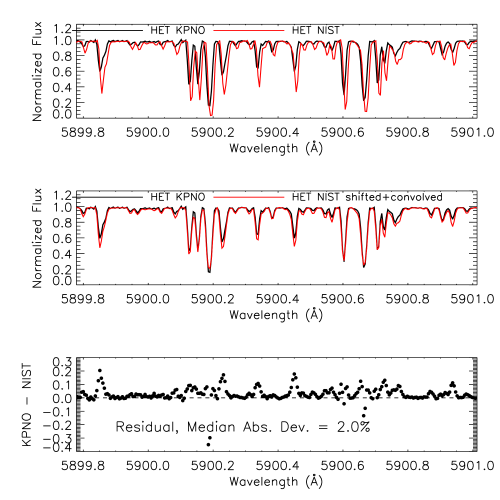
Figure 1: Comparison of the KPNO FTS spectrum (black) and the NIST FTS spectrum (red) for the HRS iodine cell for a selected 1.5Å chunk. Top: Two FTS spectra at their original resolution and original wavelength solution. Middle: Comparison of the two FTS spectra after adjusting the normalization, shifting the wavelengths, and applying convolution for the NIST spectrum to match the KPNO spectrum for a more direct comparison of line depths/ratios. Bottom: Residuals of the middle panel, i.e., the adjusted NIST spectrum minus the KPNO spectrum. The median absolute deviation between the two spectra is 0.02 (2%), though at many places, especially at line centers, the two can differ by up to 20%.

We initially suspected that the NIST spectrum was problematic. The reason is illustrated in the left panel of Figure 2, where it shows the histogram of $\chi_{\nu}^{2}$ values for fitting a selected iodine calibration frame (a $R=60,000$ lamp observation through the iodine cell) using the two FTS spectra, respectively. Each $\chi_{\nu}^{2}$ value is for a 2Å chunk in this selected iodine spectrum. It is clear that the NIST spectrum provides a worse fit.

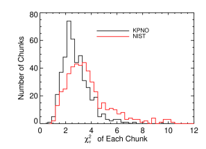
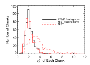
Figure 2: Both plots are histograms of $\chi_{\nu}^{2}$ values of all the spectral chunks in a single iodine calibration frame taken by HRS. Each $\chi_{\nu}^{2}$ value in the histogram represents the $\chi_{\nu}^{2}$ goodness of fit for a $\sim$2Å spectral chunk in this selected iodine spectrum (each iodine spectrum is divided into several hundred of chunks and is fitted independently using a Levenberg-Marquardt least $\chi^{2}$ fitter). Left: $\chi_{\nu}^{2}$ histograms for the fit of the iodine observation using the KPNO spectrum (black) or the NIST (red) spectrum as the model input iodine reference spectrum, respectively. The KPNO spectrum performs better. Right: $\chi_{\nu}^{2}$ histograms for the two FTS spectra, but both with spectral normalization offset for the atlas as a free parameter for each chunk. The two spectra now perform at essentially the same level. Dashed red line is the same red histogram as plotted in the left panel. Notably, the KPNO spectrum also performs better when we float the normalization offset.

Since the middle panel of Figure 1 presents a much better match between the NIST spectrum and the KPNO spectrum, we decided to add a free parameter to account for an offset term in the spectral continuum of the iodine atlas, in case any of the two FTS spectra has problems in continuum normalization from data reduction or has contamination in the continuum, for example. The right panel of Figure 2 shows the $\chi_{\nu}^{2}$ histograms for the same iodine observation using the two FTS spectra, but adding a free parameter as the normalization offset when fitting each chunk (note: this normalization offset parameter is a free parameter for each chunk, not a single global parameter). The two FTS spectra then performed at essentially the same level in term of goodness of fit for an iodine frame, with the KPNO spectrum performing slightly better.

This was both encouraging and worrisome at the same time. It was encouraging because it seemed that we have found the problem with the NIST spectrum (i.e., the continuum) and also had a solution for it. It was very worrisome because this revealed that:

• Even the KPNO spectrum performed visibly better when we floated the normalization parameter. This may suggest that there are normalization issues or low frequency errors/noise in the KPNO spectrum as well.

• Obtaining high-quality, reliable FTS spectra of iodine cell is not an easy task, and the FTS spectra cannot be naively trusted as the “ground truth”, ultra-accurate templates of the complicated iodine spectrum.

• The reason why adding a floating normalization fitted the data better might be because it accounted for optical depths difference between the atlas and the actual observations, which may be a result of changes in the cell temperature or the iodine column density.

• The forward modeling code, when floating normalization as a free parameter, could not distinguish which FTS spectrum was more accurate (by comparing $\chi_{\nu}^{2}$) even when the two FTS spectra differed as much as $\sim$5–10% at places and also had obvious line ratio differences (see comparison in bottom panel of Figure 1). However, this level of difference in FTS may affect the RV precision, and not knowing which atlas is the correct one definitely affects our ability to search for a better IP model (which was also suspected to be a limiting factor for HRS; see Wang 2016) and improve the RV precision of HRS.

It was perhaps even more alarming and more puzzling that, when we used the KPNO spectrum for the HIRES iodine cell to fit an HRS iodine frame, it yielded smaller $\chi_{\nu}^{2}$ values than using any of the other two FTS spectra of the HRS cell (Figure 3). The HRS cell’s KPNO spectrum was taken at the same time using the same FTS machine as the spectrum for the HIRES cell (Butler et al. 1996). However, the temperatures of these two cells were very different: the HIRES cell was designed to work at 50 ^∘C, while the HRS cell was designed to work at $70^{\circ}$C. A closer look revealed that the HRS KPNO spectrum and the HIRES KPNO spectrum had very similar line depths, with the HIRES cell’s FTS spectrum having slightly deeper lines (due to a higher iodine molecule column density; see more later in Section 4).

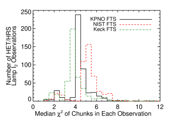
Figure 3: Comparison of the median $\chi_{\nu}^{2}$ values for the fits of HRS iodine frames using the HRS KPNO spectrum (black solid line), the HRS NIST spectrum (red dashed), and the HIRES KPNO spectrum (green dotted-dashed). Each data point represents the median of the $\chi_{\nu}^{2}$ values of all the chunks in a single iodine spectrum (these are all lamp-illuminated iodine calibration frames, not from A/B stars, i.e., through the HRS calibration fiber instead of the science fiber). Over 500 iodine calibration frames were used for this plot to ensure the statistical significance. The HIRES KPNO spectrum provided a better fit than the both HRS FTS spectra when fitting HRS iodine observations.

The findings above prompted us to seek an independent way to perform quality checks for any FTS spectrum — not just comparing their relative qualities or performances. One natural choice would be to obtain spectra taken with high-resolution echelle spectrographs, which are measurements of the iodine spectrum directly in the real wavelength space instead of in the Fourier space, and thus they could serve as good reference spectra as they would suffer from different types of error compared with FTS spectra. Since FTS spectra are usually at a very high spectral resolution ($200,000$–$500,000$), this limited our choice to essentially only one spectrograph at the time (circa 2014) — the TS12 configuration of the Tull Spectrograph One (TS1) at the 2.7-meter Harlan J. Smith Telescope at McDonald Observatory (Tull et al. 1995).

Our goal for taking spectra with TS12 was to answer the following questions: which FTS spectrum better describes the HRS iodine cell: the KPNO one, or the NIST one? And why? Why did the FTS spectrum for the HIRES cell work even better than the HRS FTS spectra? While adding an additional normalization offset parameter provided better fits for the iodine frames, we could not afford to add such an additional parameter when extracting RVs from star plus iodine spectral data – this normalization offset parameter would be degenerate with the Doppler shift and the wavelength solution parameters and thus would lead to a decrease in the RV precision. Therefore, we needed to resolve the issue instead of adding an additional free parameter to mend the FTS spectrum.

3 Validating FTS spectra of Iodine Cells using the Tull Spectrograph One

To break the tie between various FTS spectra, we used the TS12 configuration of the Tull Spectrograph One (Tull 1972). The Tull spectrograph with TS12 was the highest resolution spectrograph on sky at the time of our experiment around 2013. It employs a double pass on the echelle grating to achieve a resolution of $\sim$500,000, based on ThAr line measurements taken during our observations. TS12 was frequently used for studying lines of the interstellar medium in the 1990s (e.g., Sembach et al. 1996), and was rarely used in the recent years.

We had two rounds of TS12 observing session, both during day time and when the telescope was scheduled for Cassegrain instruments and the Tull Spectrograph in the coudé room was free for use. For the first run (from September 7 to September 9, 2013; done by Sharon X. Wang and Ming Zhao), we measured the iodine absorption spectrum for the iodine cell of the Sandiford Spectrograph at the 2.1-meter telescope at McDonald Observatory, because the HRS cell was unavailable (it was still under active use for planet search programs at HET). The main purpose of the first run was to validate the quality of the TS12 spectrum and whether we could use it to validate the FTS spectra. The Sandiford cell also had a KPNO FTS spectrum, which was taken together with the KPNO spectrum of the HRS cell in 1993, so it also served the purpose of testing the overall quality of the KPNO FTS spectra.

In the second TS12 run, we measured the spectrum for the HRS iodine cell in its original enclosure and temperature controller (the enclosure and the thermal control system have been rebuilt since then). We also took spectra of other iodine cells, including the MINERVA (Swift et al. 2015) iodine cell and the iodine cell used at the McDonald 2.7-meter Smith telescope. The run was from October 13 through October 16, 2014 and was carried out by Ming Zhao, Kimberly M. S. Cartier, and Joseph R. Schmitt, with the help of Phillip MacQueen in setting up the cells.

The hardware settings and data reduction methods are the same for both runs, which are described below.

Hardware Settings: We used the TS12 configuration of the Tull Spectrograph One, and the specific instrument settings we used are listed in Table 1. Slit #23 is chosen to maximize SNR while maintaining sufficient resolution — it is among the longest slits and is the second narrowest slit. The slit is $0\arcsec.32$ wide and $30\arcsec$ tall, or 5.8 by 543 pixels, given the plate scale of TS12 with the TK4 CCD being $0.55\arcsec$ per pixel. The Sandiford cell was kept at a temperature of 49.9–50.1^∘C, the same as its working temperature for RV observations and also the same as its temperature when the KPNO was taken (50 ^∘C). The HRS cell was measured at four different temperatures: room temperature, 50 ^∘C, 60 ^∘C, and 70 ^∘C (its working temperature).

Table 1: Hardware Settings for TS12

Tull Spectrograph One, TS12, Coude107
Echelle	E1
Cross Disperser	c
CCD	TK4, 1024$\times$1056
On-chip Binning	1$\times$1
Slit	#23 (L$\times$W $=30\arcsec\times 0\arcsec.32$)

Observations: A single exposure frame for the iodine spectrum covers about 1.9Å (Figure 4). The dispersion direction runs vertically along the chip with increasing wavelength when increasing the $y$-axis pixel. The dispersion scale is about 0.002Å per pixel, with $\sim$7 pixels per resolution element. We immediately preceded or followed each exposure with a flat fielding frame in the same echelle and cross disperser positions as the iodine frame. The exposure times for the iodine and flat frames are both 45 seconds (90 seconds for the HRS cell) to achieve a signal-to-noise ratio (SNR) of 160 per CCD pixel (again, higher for the HRS cell). Neighboring frames differ by about 1Å in absolute wavelength, leaving ample overlapping regions between frames for post-reduction stitching of the spectrum. If prominent Solar or ThAr line was predicted within the wavelength coverage of a frame, then we also took a Solar or ThAr frame to verify the rough wavelength solution. The exposure times for these Solar or ThAr frames varied — typically from a couple minutes to up to 10 minutes. We took dark frames (45s each, about 10 frames) in the morning at the beginning of each day.

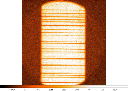
Figure 4: One raw image frame taken using the TS12 setting of Tull Spectrograph One. It contains about 1.9Å of iodine absorption spectrum.

Reduction: We combined and averaged all available dark frames and created a master dark frame. Then we subtracted the master dark from all flat and iodine frames. After outlier rejection (cosmic rays, chip defects, etc.), we modeled the scattered light for each row of pixels by using the region on the CCD outside of the slit image. To estimate the scattered light in an image row, we added the flux in 160 neighboring rows (80 above and 80 below the target row) along the column direction (i.e., the dispersion direction). We then fitted a third order polynomial to the added flux outside of the slit image region to construct a model of the scattered light. Then we evaluated the values of scattered light within the slit image region using the best-fit polynomial and subtracted it off. Both the flat and iodine frames have scattered light removed. Then we normalized the flat frames and divided each iodine frame by its associated normalized flat (for the slit image regions only).

Extraction: As the slit does not lie perfectly along the $x$-axis direction on the chip, we rectified the image before extraction by first taking columns along the dispersion direction and cross-correlating these columns. The relative shift between columns was determined via oversampling the two spectra by a factor of 10, and then performing cross correlation to determine the amount of shift by fitting a Moffat function to the cross correlation function. Then we interpolated the columns via spline interpolation to a common pixel grid after shifting them to create an aligned image. We then added the flux along the row direction (i.e., cross-dispersion direction) and obtained the reduced, extracted spectrum. Each spectrum is then normalized by dividing the estimated continuum (top 5% counts). Due to lower quality of scattered light removal near the edge of the chip, we discarded the top 80 and bottom 80 rows of pixels. Thus the extracted spectrum from each frame is about 1.6Å across (instead of 1.9Å). The reduced frames are then stitched together by finding the overlapping region through cross correlation of each pair of neighboring frames while taking into account the changes and differences of dispersion scales across frames.

Mapping onto FTS: The extracted TS12 spectra are not wavelength calibrated naturally like the FTS spectra. To compare with the FTS spectra, we divided the TS12 spectrum into 2Å chunks and projected each chunk onto the FTS spectrum via cross correlation. In this way we obtained the absolute wavelength solution and dispersion scale (as set by the wavelength solution of the FTS spectrum) for the TS12 spectrum.

The results from our first TS12 run using the Sandiford cell demonstrated that an iodine cell spectrum taken with TS12 has the same quality as an FTS spectrum to serve as the “true solution” of the iodine spectrum in the forward modeling process for RV extraction (although a wavelength solution would have to be derived). The left panel of Figure 5 shows a direct comparison of the reduced TS12 spectrum (a random 2Å chunk) with the KPNO FTS spectrum, at their native resolutions.

To make a more direct comparison and also to see the differences of the two spectra (if any) would make a significant impact when fitting a typical iodine observation with a spectral resolution of $60,000$, we degraded the resolution of both spectra to $60,000$ by convolving them with a Gaussian IP. The right panel of Figure 5 illustrates the comparison of the two spectra at $R\sim 60,000$, with residuals of the TS12 spectrum minus the KPNO FTS spectrum plotted in the bottom panel. The two spectra differ by a median absolute deviation of 0.3% ($0.4\%$ for the entire $\sim$30Å spectrum available as shown in Figure 6). As the TS12 spectrum has a SNR of about 160 per pixel and we have convolved the comparison spectrum down to $R\sim 60,000$, the expected shot noise should be $\sim 1/160\times\sqrt{450,000/60,000}=0.23\%$. The additional $\sim 0.1\%$–$0.2\%$ of noise may come from flat fielding, scattered light removal, cosmic ray removal and interpolation between pixels, stitching of spectra, projection onto the FTS spectrum and interpolation for comparison purposes, and so on.

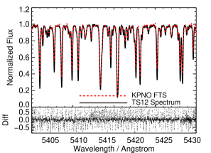
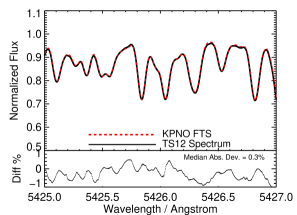
Figure 5: Comparison of the Sandiford iodine cell KPNO FTS spectrum and the spectrum taken with TS12. Left: Comparison of the two spectra in their native resolutions (both about $400,000$–$500,000$). Right: Comparison of the two spectra convolved down to about $60,000$ resolution, which is the resolution of typical iodine observations or radial velocity observations (star$+$iodine). Bottom panel shows the residuals in percentage of the TS12 spectrum minus the KPNO spectrum, with a median absolute deviation of 0.3%.

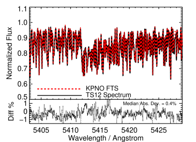
Figure 6: The same as the right panel of Figure 5, the KPNO spectrum and the TS12 spectrum for the Sandiford cell both at $60,000$, but for the entire $\sim$30Å TS12 spectrum available.

After demonstrating that we can use TS12 spectrum to validate FTS spectra using the Sandiford cell, we performed our second TS12 run with the HRS cell (and the 2.7-meter cell and the MINERVA cell). For the 2.7-meter cell, its TS12 spectrum matches very well to its FTS atlas, similar to the results with the Sandiford cell, proving again that TS12 is an appropriate tool for validating FTS atlases. For the HRS iodine cell, the story is very different and the results are very informative:

(1) Assuming that the HRS cell temperature control was reliable during our TS12 run, then temperature change on the order of 5–10 ^∘C in iodine cell should induce a visible change in the absorption spectrum (right panel of Figure 7). On the other hand, the temperature of the iodine gas in the cell does not seem to be at $70^{\circ}$C as set by the temperature controller during the NIST spectrum (left panel of Figure 7; see more in Section 4). This could explain the difference between HRS cell’s NIST spectrum and the KPNO spectrum. The HRS cell during the NIST FTS scan appears to have stayed at a temperature higher than $70^{\circ}$C during the entire FTS scan, at the same high temperature with three different temperature settings at 65, 70, and $75^{\circ}$C. The HIRES cell was also scanned at three different temperatures (50, 60, and 70 ^∘C) at KPNO in 1993, and there are also visible differences between these three sets of FTS spectra, unlike HRS cell’s NIST spectrum.

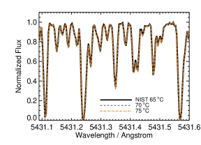
(a)

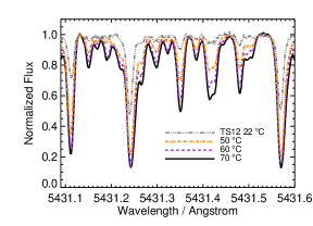
(b)

Figure 7: Left: HRS cell NIST FTS spectrum at three different temperatures. Right: HRS cell TS12 spectra at four different temperatures for the same wavelength region, which, unlike the NIST FTS spectra, shows significant difference when the temperature of the cell changes by 10 ^∘C.

(2) The TS12 spectrum at $70^{\circ}$C matches better with the more recent but potentially problematic NIST FTS spectrum (Figure 8). In fact, the TS12 spectrum does not match the NIST FTS spectrum well enough given the high SNR nature of both spectra, so they are actually inconsistent, although less so compared with the KPNO FTS spectrum. If the HRS cell was indeed at $70^{\circ}$C during the KPNO spectrum, as we have seen that the KPNO FTS spectra are validated using the TS12 spectra for both the Sandiford cell and the 2.7-meter cell, then Figure 8 suggested that the HRS cell was not at its set temperature of $70^{\circ}$C during either the TS12 run or the NIST spectrum. Or, perhaps the amount of iodine vapor was somehow different.

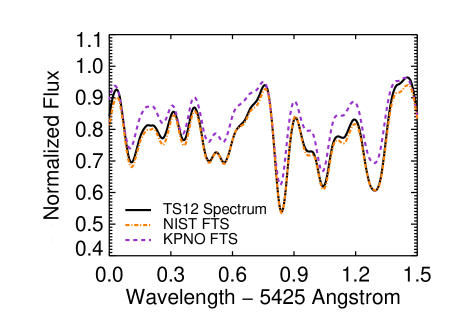
Figure 8: TS12 spectrum (black solid line) vs. NIST FTS (orange dot-dashed) vs. KPNO FTS (purple dashed) for the HRS iodine cell at 70 ^∘C, all convolved down to a resolution of R $=$ 60k (the same as a typical HRS observation) for comparison purposes. The TS12 spectrum matches the NIST FTS better, having deeper lines compared to the original KPNO FTS. The remaining difference between NIST FTS and the TS12 spectrum might be due to differences in cell temperatures or other changes with the cell.

These results prompted us to resolve for a second route to try to break the tie: using synthetic iodine absorption spectra, which is described in the next subsection.

4 Measuring iodine cell temperatures using IodineSpec5

Using the TS12 spectra, we found that the temperature of the iodine gas in the cell might not be the same one as reported by the temperature controller. However, we still could not break the tie between the KPNO spectrum and the NIST spectrum for the HRS cell: the KPNO spectrum provided a better fit to real observed data, but the TS12 spectrum showed us that the NIST spectrum looked closer to the “truth” as defined by TS12 (if that was the truth). Nor did we understand why the KPNO spectrum for the HIRES cell worked the best for HRS data.

To answer these questions, we found a second venue that provided reliable, ultra-high resolution, and wavelength calibrated iodine atlas – a theoretical code that computes synthetic iodine transmission spectrum (at any specified temperature) based on both quantum physics and empirical calibrations (IodineSpec5; Knöckel et al. 2004). The direct output of the code contains arrays of wave numbers and, effectively, opacity ($\alpha$) for user-specified iodine isotope mix (for our purposes we only add ${}^{127}I_{2}$), temperature, wave number range, and a line broadening kernel (we chose thermal/Gaussian). To use the output of IodineSpec5 to fit an actual iodine absorption spectrum, there are two parameters: gas temperature and a constant which scales with iodine molecular column density, which we simply refer to as the column density hereafter.

A quick comparison between the NIST spectrum and the IodineSpec5 models revealed that the NIST spectrum seems to be around 110 ^∘C, based on visually examining the line ratios (Figure 9). However, the synthetic iodine spectrum and the FTS spectra have different broadening kernels. In order to “fit” the NIST spectrum with the synthetic spectra at various temperatures, we convolved the NIST spectrum with a single Gaussian kernel with $\sigma=0.0078$ (roughly at $R=$ 200,000 to match the HIRES cell KPNO spectrum for comparison and illustration purposes). Except for the HIRES cell’s FTS spectrum, we did the same to lower the resolution of other FTS spectra or TS12 spectra when using IodineSpec5 to determine their best-fit temperatures. There are four parameters in our fit: temperature, column density, resolution ($\sigma$ for the single Gaussian kernel to convolve with the synthetic IodineSpec5 spectrum), and a wavelength shift (since it is common for different FTS spectra to have offsets in wavelengths due to calibration errors). We first optimized the column density, $\sigma$, and the wavelength shift while fixing the temperature (using a levenberg-Marquardt least-$\chi^{2}$ fitter with the mpfitfun package in IDL), and then we compare the goodness of fit of each model at different temperatures to determine which temperature best describes the FTS spectrum or the TS12 spectrum at hand. The reason for this two-step optimization is that we had to generate the IodineSpec5 model spectra on a discrete temperature grid.

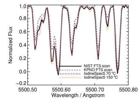
Figure 9: NIST FTS (black solid line) and KPNO FTS (gray dashed) spectra for the HRS cell compared with theoretically computed iodine lines by IodineSpec5 at 70 ^∘C (purple dot-dashed) and 150 ^∘C (orange dotted). All spectra are at their original resolution. There are two free parameters for the theoretical lines: temperature and iodine column density. For this plot, we optimized the iodine column density for the theoretical lines at both temperatures to try to match the NIST FTS. As illustrated, neither the 70 ^∘C nor the 150 ^∘C spectrum can produce a good match, and, as shown later, the best-fit temperature is around 110 ^∘C. Note that the theoretical lines and the NIST spectrum have different broadening kernels.

We first fitted the HIRES cell KPNO FTS spectrum, whose temperature was known (50 ^∘C) and probably reliable. We knew that this FTS spectrum was probably true to its reported temperature since the HIRES iodine atlas fitted the data very well, as described in the previous section. Choosing a region with temperature-sensitive lines, we found the best-fit temperature for the HIRES cell’s KPNO spectrum was 55 ^∘C, although synthetic spectra ranging from 40-70 ^∘C all had a similar goodness of fit and they were hard to distinguish by eye (column density and temperature are parameters with some degeneracy in the fitting). We thus conclude that IodineSpec5 is reliable for estimating temperatures for iodine FTS spectra, at least to an accuracy of 5-10 ^∘C.

We then fitted the NIST spectrum, which has the highest SNR and the highest resolution among all FTS spectra and the TS12 spectra (we also had a rough idea about its temperature from the visual comparison in Figure 9). The results are shown in Figure 10, where the top panel shows the best-fit models at different temperatures, and the bottom panel compares the NIST spectrum with its best-fit model at 110 ^∘C, the KPNO spectrum, and the HIRES cell’s KPNO spectrum.

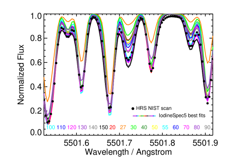
(a)

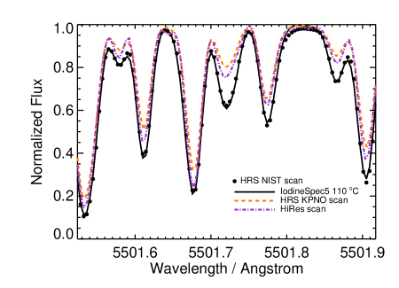
(b)

Figure 10: Top: Fitting the HRS NIST spectrum (black dots; when temperature was set at 70 ^∘C) with the best-fit IodineSpec5 synthetic iodine lines at various temperatures (colored lines, with corresponding temperatures labeled in colored numbers). Bottom: The HRS NIST spectrum (black dots) over-plotted with the best-fit IodineSpec5 model (black solid line; at 110 ^∘C) and the KPNO FTS spectra for the HRS cell (orange dashed) and the HIRES cell (purple dot-dashed). All spectra in both panels are convolved down to a resolution of 200,000 (roughly at the HIRES cell’s KPNO FTS spectral resolution) to minimize the difference in line shapes due to IP differences between the FTS spectra (with a sinc function IP) and also the synthetic spectrum (with only natural thermal broadening kernels).

When we fitted the HRS KPNO spectrum, the high degeneracy between column density and temperature hindered us from getting an accurate estimate for the temperature. Models in 40-80 ^∘C appear to fit equally well with varying column densities. However, only the fit at $70^{\circ}$C has the same column density as the best-fit value derived from the NIST fit. We thus fixed the column density in our fits for the HRS cell’s KPNO spectrum, and the best-fit temperature came out to be $70^{\circ}$C, as expected. Therefore, we conclude that during the NIST FTS spectrum, the HRS cell was at a different gas temperature than the set temperature of $70^{\circ}$C, and the cell was at the right temperature during the KPNO spectrum.

But how about the TS12 spectrum? Again, using the best-fit column density derived from our best-fits for the NIST and KPNO FTS spectra, we estimated the temperatures for the three TS12 spectra with temperatures reported to be set at 50, 60, and 70 ^∘C. The best-fit temperature turns out to be 55 ^∘C for claimed 50 ^∘C TS12 spectrum, 80 ^∘C for the 60 ^∘C one, and 100 ^∘C for the 70 ^∘C one. The results from fitting the “70 ^∘C” TS12 spectrum are illustrated in Figure 11.

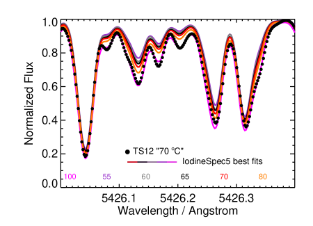
(a)

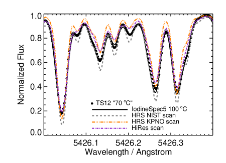
(b)

Figure 11: Top: Fitting the TS12 spectrum (temperature set at 70 ^∘C; black dots) with IodineSpec5 models, with fixed column density derived from the best fits for the HRS KPNO and NIST FTS spectra. Again, colored lines are best-fit IodineSpec5 models with different temperatures labeled in colored numbers. Bottom: The best-fit temperature for the TS12 spectrum is 100 ^∘C (black solid line). It is clearly at a lower temperature than the NIST spectrum (gray dashed) but at a higher one than the KPNO spectrum (orange triple-dot-dashed). For comparison, the HIRES cell’s FTS spectrum is also plotted (purple dot-dashed). Again, all spectra in both panels were convolved down to $R=$ 200,000.

These findings on the HRS cell temperatures could explain the fits to the observed data. If the HRS cell was kept at a higher temperature (e.g., $\sim 100^{\circ}$C) instead of $70^{\circ}$C when it was in active use for precise RV calibration (despite what the temperature control reported), or if the actual temperature of the gas in the cell changed over time, then the KPNO FTS spectrum, which was done at $70^{\circ}$C, certainly cannot fit the observed data very well or provide precise calibrations to measure RVs to the same level as HIRES, which had a correct iodine atlas. The bottom panel of Figure 11 provided some clues for why the HIRES cell’s FTS spectrum provided the best fits to HRS data (Figure 3) – if the gas temperature was between 70 and 110 ^∘C during actual HRS observations (and perhaps more often closer to 70 ^∘C), then an iodine atlas which has line depths in between the KPNO (at 70 ^∘C) and the NIST (at 110 ^∘C) FTS spectra would provide a better fit than both, which the HIRES cell’s FTS spectrum happened to satisfy by coincidence.

Why was the temperature of the iodine gas in the cell higher than 70 ^∘C as set by its temperature controller? We explore potential causes for the rise of HRS cell temperature in the next section.

5 Cause for a Higher Iodine Gas Temperature

Throughout the FTS spectra at NIST and our TS12 observation, the readings of the temperature probe on the HRS iodine cell stayed at 70 ^∘C. However, as discussed above, the temperature of the iodine gas in the cell appears to be higher: 110 ^∘C for the NIST FTS spectrum and 100 ^∘C for the TS12 spectrum with the $70^{\circ}$C setting.

One potential explanation for this temperature discrepancy is that the temperature probe was malfunctioning. It does not report a true temperature but is biased towards a lower reading than the actual temperature. In preparation for HRS’s instrumental upgrade, the thermal enclosure and temperature control system was rebuilt since our TS12 experiment, so fortunately this old thermal system, functioning properly or not, would no longer affect any future HET’s RV observations.

An alternative explanation is that the temperature probe was working, but either there was a temperature gradient in the cell, or the gas was at a higher temperature while the glass cell stayed cool. These two alternative scenarios seem plausible, especially as an explanation for the high temperature of the gas for the NIST FTS spectra. We noticed that the halogen lamp used for the NIST spectrum, which provided the continuum emission shining through the iodine cell, was exceptionally bright compared with other commonly used halogen lamps, probably in order to provide the high SNR needed for the high resolution FTS spectra. It was a lamp with a power of $1\ kW$ and the room was considerably warmed up by this lamp. We discuss the possibility of these two scenarios below through order-of-magnitude estimates. The properties of the HRS iodine cell are as follows: it is a Pyrex glass cylinder cell, 70 mm in length and 50 mm in diameter with 6.35 mm thick windows. The cell is shorter than the typical 4 inch cell (such as the HIRES cell) in order to fit into the spectrograph, and as a result, it was run at a higher temperature of 70 ^∘C than the HIRES cell to compensate for the shorter column length. We used a gas pressure similar to the HIRES cell, at 0.01 atm at its operating temperature (Butler et al. 1996;), which may not be accurate for the HRS cell but should suffice for our order-of-magnitude calculations.

5.1 Temperature Gradient in the Glass

We first explore if shining a very bright light, such as using the Xenon lamp at NIST, at the HRS iodine cell would induce a large enough temperature gradient in the cell glass (Pyrex) to explain the difference between the gas temperature (110 ^∘C) and the temperature probe reading (70 ^∘C, assuming correct). The HRS cell had one temperature probe taped at one of the side windows of the cell (the HIRES cell has two probes: one in the middle within the heating wraps and one at the window of the cell). A temperature gradient in the glass cell could mean that the heated glass on one side can bring the gas inside to a higher temperature, while the glass on the other side with the temperature probe stays at $70^{\circ}$C. To sustain a temperature gradient, there needs to be a continuous heat input, which would be the Xe lamp shining on the cell at NIST. According to the law of heat conduction, or Fourier’s law (in its 1-D differential form), the temperature gradient can be estimated via:

$$q=-k\frac{dT}{dx},$$ (1)

where $q$ is the heat flux density in $W/m^{2}$, $k$ is the thermal conductivity of the material in $W/m\cdot K$, and $dT/dx$ is the temperature gradient in $K/m$.

The heat flux density coming from the Xe lamp can be derived by

$$q=I_{\rm lamp}\cdot\Delta\lambda\cdot f_{\rm absorption},$$ (2)

where $I_{\rm lamp}=200$ $mW/m^{2}/$nm is the irradiance of the Xe lamp used in the scan for the wavelength region of 400–700 nm at a distance of 0.5 m, which is set by two colored glass filters (GG495 and BG40) that restrict the emission to the iodine region. Therefore $\Delta\lambda$ would be 300 nm. We assume a distance of 0.5 m here since we do not have the exact measurement of the setup at the NIST FTS scan, but this number should be close enough for the purpose of this estimate. $f_{\rm absorption}$ is the fraction of radiation absorbed by the glass.

To estimate $f_{\rm absorption}$, we need the absorption spectrum of cell material, Pyrex. Pyrex is largely transparent in the optical, but it has an absorption feature near 2.7 $\mu$m and it heavily absorbs UV light short of 300 nm and IR light longer than 5 $\mu$m. Considering the filters used between the lamp and the iodine cell at the NIST scan, $f_{\rm absorption}$ would mostly come from 400–700 nm region, where its average $f_{\rm absorption}$ is roughly 8%. Therefore, the heat flux density coming from the Xe lamp would be $q=4.8~{}W/m^{2}$.

For a broader application of our estimate here, we also want to consider other common setups at astronomical observatories. Here we also estimate the heat flux density coming from a commonly used halogen lamp at a distance of 1 m with just a UV filter in between the lamp and the iodine cell. The heat flux density coming from the halogen lamp can be derived by

$$q=P_{\rm lamp}\cdot f_{\rm beaming}\cdot f_{\rm absorption}/4\pi D^{2},$$ (3)

where $P_{\rm lamp}=1\ kW$ is the power of the lamp, $f_{\rm beaming}$ is the beaming factor of the lamp (as it is not isotropically radiating towards all directions), $f_{\rm absorption}$ is the fraction of radiation absorbed by the glass, and $D$ is the distance from the lamp to the cell.

For a rough estimate, here we assume $f_{\rm beaming}=3$ (meaning the light from the lamp is filling a solid angle of $4\pi/3$) and $D=1$ m. To estimate $f_{\rm absorption}$, we assume the halogen lamp spectrum is a black-body spectrum with peak around $1\mu$m, which is typical for this type of lamps. Considering the UV filter between the lamp and the iodine cell, $f_{\rm absorption}$ would mostly come from IR. This fraction can be estimated by numerically integrate the Planck function for the intervals $[2.5,3.0]\ \mu$m and $[5.0,\inf]\ \mu$m, and $f_{\rm absorption}$ turns out to be about 6% of the total lamp emission. From these numbers, $q$ is estimated to be 14.3 $W/m^{2}$. Since this number is much larger than the heat flux density from the Xe lamp at NIST, we carry on our calculation using this number from the halogen lamp setup. As shown later, this heat flux density is not large enough to explain the temperature anomaly we saw, and therefore the same conclusion holds for the NIST setup using Xe lamp.

Now we continue with our estimate for heat conduction in the iodine cell. The thermal conductivity ($k$) of Pyrex is a well known number, as it is a widely used and manufactured material, and it is about $k=1.1\ W/m\cdot K$.

Plugging in $q=14.3~{}W/m^{2}$, $k$, and using $dx=7$ cm or 0.07 m (the length of the iodine cell), $dT$ turns out to be about 1.0 $K$. Considering the fact that the light was shining on the window of the glass cell and then being conducted down the thin cylinder shell, and perhaps the distance between the lamp and the cell $D$ was smaller than 1 meter, $q$ may be boosted by a factor of a few (assuming the thickness of the glass cylinder is a couple mm), up to perhaps 10 $K$. Therefore, we conclude that the temperature gradient is unlikely to be as large as $40\ ^{\circ}$C, though not completely ruled out given our crude method of estimation. In any case, this amount of heat may not be large enough to heat the glass from $70\ ^{\circ}$C to $110\ ^{\circ}$C, or even sustain the high temperature of the glass, because of its relatively high cooling rate estimated below.

First, the amount of input energy from the lamp is probably too small to cause a significant temperature rise in the glass. Using the specific heat of Pyrex, $C_{P}=0.75\ J/g\cdot K$, assuming the weight of the glass cell to be $M_{\rm glass}=100\ g$, and using an input power of $q\times\pi r^{2}$, where $r=0.025$ m is the radius of the iodine cell window, the rate of the temperature rise in Pyrex from heating of the lamp is:

$$dT/dt=q\cdot\pi r^{2}/C_{P}M_{\rm glass}=3.8\times 10^{-4}\ K/s.$$ (4)

Even assuming the glass does not cool, this means the temperature would only rise for about 4 $K$ in an hour.

Second, the thermal radiation from the glass alone would cool the glass off fast enough. At $T=100\ ^{\circ}$C $=375.15\ K$, the thermal radiation has a power of $\sigma T^{4}=1123\ W/m^{2}$ – much larger than the input energy from the halogen lamp (recall that $q=14.3\ W/m^{2}$). Even considering that the glass was wrapped in thermal insulators and only its two windows were exposed to the air, the thermal radiation would still be large enough to cool the glass down fast enough and prevent continuous rising of the glass temperature (which would be too slow anyway, as argued above).

Therefore, if the temperature probe was working, it was mostly likely that the entire glass stayed at its reported temperature instead of having a temperature gradient as large as $40\ ^{\circ}$C during the NIST FTS spectra.

5.2 Heated Gas within a Cooler Glass

Next, we investigate the temperature of the iodine gas inside the cell and whether it might be decoupled in temperature from its glass cell container. If the gas was heated up to a higher temperature without the glass cell being heated up considerably, then perhaps the temperature probe was working but it was only reporting the temperature of the glass instead the gas. Below we argue that this is unlikely to be the case.

First, the small mean free path of the iodine molecule in the cell suggests that they primarily thermalize with themselves and then with the glass, which seems to support the hypothesis of the thermal decoupling between the gas and the glass, but we argue later with other evidence that is against this hypothesis. The mean free path of iodine molecules is estimated by using ideal gas assumption:

$$\lambda=(\sqrt{2}\sigma\cdot n)^{-1}=\frac{k_{B}T}{\sqrt{2}\pi d^{2}P},$$ (5)

where $\sigma$ is the interaction cross section of the molecule, $n$ is the number density of molecules, $k_{B}$ is the Boltzmann constant, $d$ is the effective diameter of the molecule, and $P$ is the pressure of the gas. The iodine gas in the cell has a pressure of about 0.01 atm or 1 kPa (Butler et al. 1996), at a temperature of $110\ ^{\circ}$C or 385 $K$, with an effective diameter of about 5Å (Juhola 1975; Topley 1926). Using these numbers, the mean free path is estimated to be 4.8 $\mu$m, much smaller than the size of the glass cell. This means that the gas is not tenuous enough so that their thermalization is completely dominated by the glass enclosure. But more evidence is needed to support this hypothesis of thermal decoupling.

Second, assuming the gas was thermally decoupled from the glass, then what was the dominating heating source for the iodine gas? There were three heating sources for the gas during the NIST FTS scan: (1) the heat from the temperature enclosure heater conducted via the glass, (2) the heat from the halogen lamp absorbed by the glass then conducted to the gas, and (3) the direct radiation from the halogen lamp. For heat source (1), according to the calculation in the previous subsection and our assumption here of a working temperature probe, the glass cell would have stayed at $70\ ^{\circ}$C, so it was not heating up the gas to a higher temperature.

For heat source (2), the additional heat received by the glass from the lamp, we have worked out the amount to be 14.3 $W/m^{2}$ in the previous subsection. This is too small to heat up the glass, but could this small amount of heat be conducted to the iodine gas inside and heat it up? There are four outlets for this received energy: radiative cooling of the glass, thermal conduction to the rest of the glass cell, thermal conduction to the air, and thermal conduction to the iodine gas within. The thermal conductivity of the Pyrex glass is 1.14 $W/m\cdot K$, as mentioned before, and the thermal conductivity of the air is about $2\times 10^{-2}\ W/m\cdot K$. Both are much larger than the thermal conductivity of the iodine gas, which is on the order of $10^{-4}$-$10^{-3}\ W/m\cdot K$. This means that the glass will primarily conduct along the glass cell itself, and then a smaller fraction to the air, and then an even smaller fraction to the iodine gas. Considering the factor of $100-1000$ difference in thermal conductivity between glass/air and iodine gas, probably only a $<1$% of the heat input $q=14.3\ W/m^{2}$ is being conducted to the iodine gas, i.e., $<0.14\ W/m^{2}$. This number would be even smaller if thermal radiation of the glass is considered.

For heat source (3), the direct radiation from the halogen lamp, we estimate below that it would be contributing a power of $q\sim 1.7\ W/m^{2}$ (or $3.3\ mW$, given the radius of the cell window is 2.5 cm) to the iodine gas. This number is estimated by using equation 3 for $q$, but substituting $f_{\rm absorption}$ with $0.3\times 0.024$, 0.3 being the approximate fraction of light the iodine molecules absorbs in the optical window $[500,650]$ nm, and 0.024 is the fraction of energy emitted by the halogen lamp in this wavelength range (again assuming its a blackbody as before). If the gas was heated to above $70\ ^{\circ}$C, this would be the primary source of heating. However, this amount of power is probably too small. Again, the thermal radiation of any $100\ ^{\circ}$C material is $1123\ W/m^{2}$, as calculated above, much larger than the $1.7W/m^{2}$ input power. Plus the iodine gas also cools via band emission (Waser & Wieland 1947). Therefore, it is very unlikely that the iodine gas was actually heated up to $110\ ^{\circ}$C because of the halogen lamp.

Additionally, although the thermalization between the glass and the gas might be slow, it would not be at a longer timescale than the FTS scan (about a few hours). The specific heat of Pyrex is $C_{P}=0.75\ J/g\cdot K$, and assuming the iodine gas is at $T=100\ ^{\circ}$C and the glass is at $T=70\ ^{\circ}$C:

$$dT/dt=\frac{(\sigma T_{\rm gas}^{4}-\sigma T_{\rm glass}^{4})\cdot A}{C_{P}M_{\rm glass}}=0.05\ K/s,$$ (6)

where $A$ is the surface area of the iodine cell, on the order of $10^{-2}\ m^{2}$. This is probably a lower limit, because the iodine gas would also emit band emission which will be absorbed by the glass (in UV) and the glass would not cool very efficiently as it was wrapped in thermal insulators. Therefore, if the gas was heated up to $100\ ^{\circ}$C, then the glass would be heated up by the gas fast enough to change the reading on the temperature probe on a timescale of minutes.

To summarize the findings above, it is highly unlikely that the glass underneath the temperature probe was at $70\ ^{\circ}$C while the iodine gas inside was at $110\ ^{\circ}$C. This means that a biased temperature probe and/or a malfunctioning temperature controller is the most likely explanation for high temperatures we found for the NIST FTS spectra and the TS12 spectra in Section 4. One possible scenarios is that, if the heater of the temperature controller was turned on the entire time, the temperature of the cell and the gas would have kept rising until they had reached a thermal equilibrium, for example, with its thermal radiation. If this were the case, then the power of the temperature controller heater would be $1123W/m^{2}\times 10^{-2}\ m^{2}=11\ W$, which sounds plausible. This could explain why all three NIST spectra, supposedly taken at 65, 70, and 75 ^∘C, all seemed to be at $110\ ^{\circ}$C instead.

We conclude that the difference between the iodine atlas and the iodine observations was a result of mismatched iodine gas temperatures, and this would be the most likely culprit behind HRS’s under-performance in terms of RV precision compared with HIRES.

6 Summary and Conclusion

Iodine cell atlases are critical for obtaining precise RVs with iodine-calibrated high resolution spectrographs. In this paper, we investigated the reason behind the difference between the two iodine FTS atlases of the HET HRS iodine cell, and concluded that it was due to a temperature difference of the iodine gas caused by a malfunctioning thermal enclosure and controller.

We have established a new method for validating iodine FTS atlases or performing quality checks of iodine cells in general — using spectra taken by the ultra-high resolution arm, TS12, of the Tull Spectrograph One at McDonald Observatory. We have demonstrated that the TS12 spectra have similar quality to the FTS spectra, and in principle, the TS12 spectra could serve as the “true solution” of the iodine spectrum in forward modeling if wavelength calibrated. We have also found that the software IodineSpec5 is very useful for determining the iodine gas temperature through fitting theoretically computed iodine absorption spectra to high SNR, high resolution iodine spectra, such as FTS spectra or the TS12 spectra. We also explored and ruled out two alternative explanations for the high temperature we found for the HRS iodine cell besides a malfunctioning temperature controller: a temperature gradient in the glass cell and thermal decoupling of the iodine gas and the glass cell.

Based on our work in this paper, we recommend that when diagnosing RV precision problems, it would be helpful to start with checking goodness of fit for the iodine calibration frames (lamp plus iodine, or O/B/A type star plus iodine observations). Ideally, the residuals of fits to these frames should be very close to a photon-limited precision. In addition, for iodine cells that would be exposed to extreme hot or cold weather, and especially short cells with a relatively large surface area at the windows, we recommend two temperature probes — one at the body within the heating wraps and one at one of the windows near the light path.

When the validity of the iodine atlas is in question, one could resort to IodineSpec5 to fit for the temperature to see if it is consistent with the working temperature of the cell. Besides IodineSpec5, Perdelwitz & Huke (2018) has taken a suite of iodine FTS spectra under a series of temperatures from 23 ^∘C to up to 66 ^∘C. Ultra-high resolution echelle spectra taken through TS12 or using PEPSI (Potsdam Echelle Polarimetric and Spectroscopic Instrument; Strassmeier et al. 2015) on the Large Binocular Telescope can be helpful in diagnosing iodine atlas problems as well.

In addition, given that the HIRES iodine atlas is at a resolution around 250,000, it would be reasonable to speculate that PEPSI spectrum, upon wavelength calibration with a standard atlas and/or IodineSpec5, could be used as the iodine atlas in replacement for FTS scans as well. However, since HIRES operates at a resolution of $\sim 60,000$, more tests need to be done to validate if an iodine atlas at $R\sim$250,000 would be sufficient to model spectra at higher resolutions such as $R\sim$120,000. We have also briefly explored the possibility of using the spectra generated by IodineSpec5 (with the best-fit temperature and optical depth) as the iodine atlas to fit a selected 2Å chunk (note: larger than the typical $\sim 0.5$Å areas we chose to present for temperature diagnoses in the figures) of spectrum from an iodine calibration frame taken by HRS, and concluded that the IodineSpec5 spectrum is not accurate enough to serve as an atlas.

Given that the iodine atlas provides the first order “ground truth” in precise RV work with iodine cells as calibrators, it is important to make sure that they accurately describe the state of the cell at its regular working stage. We recommend that, for iodine-calibrated precise RVs works, routine diagnostic data analysis on the iodine calibration spectra should be performed to track the quality and stability of the iodine cell as a calibrator.

References

- Baluev (2009) Baluev, R. V. 2009, MNRAS, 393, 969
- Butler et al. (1999) Butler, R. P., Marcy, G. W., Fischer, D. A., et al. 1999, ApJ, 526, 916
- Butler et al. (1996) Butler, R. P., Marcy, G. W., Williams, E., et al. 1996, PASP, 108, 500
- Butler et al. (2017) Butler, R. P., Vogt, S. S., Laughlin, G., et al. 2017, AJ, 153, 208
- Cochran et al. (2007) Cochran, W. D., Endl, M., Wittenmyer, R. A., & Bean, J. L. 2007, ApJ, 665, 1407
- Cochran et al. (2004) Cochran, W. D., Endl, M., McArthur, B., et al. 2004, ApJ, 611, L133
- Crane et al. (2010) Crane, J. D., Shectman, S. A., Butler, R. P., et al. 2010, in Proc. SPIE, Vol. 7735, Ground-based and Airborne Instrumentation for Astronomy III, 773553
- Crause et al. (2018) Crause, L. A., Butler, R. P., Nave, G., et al. 2018, in Society of Photo-Optical Instrumentation Engineers (SPIE) Conference Series, Vol. 10702, Ground-based and Airborne Instrumentation for Astronomy VII, 107025S
- Dekker et al. (2000) Dekker, H., D’Odorico, S., Kaufer, A., Delabre, B., & Kotzlowski, H. 2000, in Proc. SPIE, Vol. 4008, Optical and IR Telescope Instrumentation and Detectors, ed. M. Iye & A. F. Moorwood, 534–545
- Endl et al. (2014) Endl, M., Caldwell, D. A., Barclay, T., et al. 2014, ApJ, 795, 151
- Howard et al. (2013) Howard, A. W., Sanchis-Ojeda, R., Marcy, G. W., et al. 2013, Nature, 503, 381
- Juhola (1975) Juhola, A. 1975, Carbon, 13, 437 . http://www.sciencedirect.com/science/article/pii/0008622375900160
- Knöckel et al. (2004) Knöckel, H., Bodermann, B., & Tiemann, E. 2004, European Physical Journal D, 28, 199
- Kotani et al. (2014) Kotani, T., Tamura, M., Suto, H., et al. 2014, in Proc. SPIE, Vol. 9147, Ground-based and Airborne Instrumentation for Astronomy V, 914714
- Kuzuhara et al. (2018) Kuzuhara, M., Hirano, T., Kotani, T., et al. 2018, in Society of Photo-Optical Instrumentation Engineers (SPIE) Conference Series, Vol. 10702, Ground-based and Airborne Instrumentation for Astronomy VII, 1070260
- Mahadevan et al. (2012) Mahadevan, S., Ramsey, L., Bender, C., et al. 2012, in Proc. SPIE, Vol. 8446, Ground-based and Airborne Instrumentation for Astronomy IV, 84461S
- Marcy et al. (2014) Marcy, G. W., Isaacson, H., Howard, A. W., et al. 2014, ApJS, 210, 20
- Metcalf et al. (2019) Metcalf, A. J., Anderson, T., Bender, C. F., et al. 2019, arXiv e-prints, arXiv:1902.00500
- Nave & Sansonetti (2011) Nave, G., & Sansonetti, C. J. 2011, J. Opt. Soc. Am. B, 28, 737. http://josab.osa.org/abstract.cfm?URI=josab-28-4-737
- Niedzielski et al. (2016) Niedzielski, A., Deka-Szymankiewicz, B., Adamczyk, M., et al. 2016, A&A, 585, A73
- Pepe et al. (2013) Pepe, F., Cameron, A. C., Latham, D. W., et al. 2013, Nature, 503, 377
- Pepe et al. (2010) Pepe, F. A., Cristiani, S., Rebolo Lopez, R., et al. 2010, in Proc. SPIE, Vol. 7735, Ground-based and Airborne Instrumentation for Astronomy III, 77350F
- Perdelwitz & Huke (2018) Perdelwitz, V., & Huke, P. 2018, MNRAS, 479, 768
- Rogers (2015) Rogers, L. A. 2015, ApJ, 801, 41
- Sembach et al. (1996) Sembach, K. R., Danks, A. C., & Lambert, D. L. 1996, ApJ, 460, L61
- Strassmeier et al. (2015) Strassmeier, K. G., Ilyin, I., Järvinen, A., et al. 2015, Astronomische Nachrichten, 336, 324
- Swift et al. (2015) Swift, J. J., Bottom, M., Johnson, J. A., et al. 2015, Journal of Astronomical Telescopes, Instruments, and Systems, 1, 027002
- Topley (1926) Topley, B. 1926, Nature, 118, 802
- Tull (1972) Tull, R. G. 1972, in Auxiliary Instrumentation for Large Telescopes, 259–274
- Tull (1998) Tull, R. G. 1998, in Society of Photo-Optical Instrumentation Engineers (SPIE) Conference Series, Vol. 3355, Society of Photo-Optical Instrumentation Engineers (SPIE) Conference Series, ed. S. D’Odorico, 387–398
- Tull et al. (1995) Tull, R. G., MacQueen, P. J., Sneden, C., & Lambert, D. L. 1995, PASP, 107, 251
- Valenti et al. (1995) Valenti, J. A., Butler, R. P., & Marcy, G. W. 1995, PASP, 107, 966
- Vargaftik (1993) Vargaftik, N. 1993, Handbook of Thermal Conductivity of Liquids and Gases (Taylor & Francis). https://books.google.com/books?id=DFo1sZBwdNgC
- Vogt et al. (1994) Vogt, S. S., Allen, S. L., Bigelow, B. C., et al. 1994, in Proc. SPIE, Vol. 2198, Instrumentation in Astronomy VIII, ed. D. L. Crawford & E. R. Craine, 362
- Wang (2016) Wang, S. X. 2016, PhD thesis, The Pennsylvania State University, doi:10.5281/zenodo.58227
- Wang et al. (2012) Wang, Sharon, X., Wright, J. T., Cochran, W., et al. 2012, ApJ, 761, 46
- Waser & Wieland (1947) Waser, J., & Wieland, K. 1947, Nature, 160, 643
- Weiss & Marcy (2014) Weiss, L. M., & Marcy, G. W. 2014, ApJ, 783, L6
- Wenger et al. (2000) Wenger, M., Ochsenbein, F., Egret, D., et al. 2000, A&AS, 143, 9
- Wittenmyer et al. (2009) Wittenmyer, R. A., Endl, M., Cochran, W. D., Levison, H. F., & Henry, G. W. 2009, ApJS, 182, 97
- Wolfgang & Lopez (2015) Wolfgang, A., & Lopez, E. 2015, ApJ, 806, 183
- Wolfgang et al. (2015) Wolfgang, A., Rogers, L. A., & Ford, E. B. 2015, ArXiv e-prints, arXiv:1504.07557
- Wu & Lithwick (2013) Wu, Y., & Lithwick, Y. 2013, ApJ, 772, 74