Multiwavelength observations of GRB 140629A: ^,

Abstract

Aims. We investigate the long gamma-ray burst (GRB) 140629A through multiwavelength observations to derive the properties of the dominant jet and its host galaxy.

Methods. The afterglow and host galaxy observations were taken in the optical (Swift/UVOT and various facilities worldwide), infrared (Spitzer), and X-rays (Swift/XRT) between 40 seconds and 3 yr after the burst trigger.

Results. Polarisation observations by the MASTER telescope indicate that this burst is weakly polarised. The optical spectrum contains absorption features, from which we confirm the redshift of the GRB as originating at z=2.276$\pm$0.001. We performed spectral fitting of the X-rays to optical afterglow data and find there is no strong spectral evolution. We determine the hydrogen column density $N_{H}$ to be $7.2\times 10^{21}$cm^-2 along the line of sight. The afterglow in this burst can be explained by a blast wave jet with a long-lasting central engine expanding into a uniform medium in the slow cooling regime. At the end of energy injection, a normal decay phase is observed in both the optical and X-ray bands. An achromatic jet break is also found in the afterglow light curves $\sim$0.4 d after trigger. We fit the multiwavelength data simultaneously with a model based on a numerical simulation and find that the observations can be explained by a narrow uniform jet in a dense environment with an opening angle of $6.7^{\circ}$ viewed $3.8^{\circ}$ off-axis, which released a total energy of $1.4\times 10^{54}$erg. Using the redshift and opening angle, we find GRB 140629A follows both the Ghirlanda and Amati relations. From the peak time of the light curve, identified as the onset of the forward shock (181s after trigger), the initial Lorentz factor ($\Gamma_{0}$) is constrained in the range 82-118. Fitting the host galaxy photometry, we find the host to be a low mass, star-forming galaxy with a star formation rate of log(SFR)=$1.1_{-0.4}^{+0.9}$ M_⊙yr^-1. We obtain a value of the neutral hydrogen density by fitting the optical spectrum, log$N_{HI}=21.0\pm 0.3$, classifying this host as a damped Lyman-alpha. High ionisation lines (N V,Si IV) are also detected in the spectrum.

1 Introduction

Gamma-ray bursts (GRBs) are the most violent explosions in the Universe, releasing $10^{48}-10^{54}$ ergs (if considered isotropic) typically within a few seconds in gamma rays; but these explosions have been observed up to a few hours in some instances (Zhang et al. 2014; Greiner et al. 2015). Gamma-ray bursts can be divided into two classes depending on their duration: long (¿2 s) and short ($\leq$2 s) (Kouveliotou et al. 1993), the progenitors of which are thought to be the collapse of massive stars or the merger of two compact objects (Zhang & Mészáros 2004; Kumar & Zhang 2015), respectively. In the final stages of merger or collapse, a highly collimated ejecta is released, which has a typical opening angle $\theta_{jet}=5^{\circ}$-$10^{\circ}$ (Racusin et al. 2009; Zhang et al. 2015). An internal dissipation process within the jet is thought to produce prompt gamma-ray emission (Rees & Meszaros 1994; Kobayashi et al. 1997; Daigne & Mochkovitch 1998; Maxham & Zhang 2009; Hu et al. 2014), while a longer lived, multiwavelength afterglow is expected to be produced as the jet ploughs into the circumstellar medium (of constant density or a stellar-wind-like density; Mészáros & Rees 1997; Sari & Piran 1997). The relativistic effect implies that emission from the jet is beamed into a cone of half-opening angle 1/$\varGamma_{0}$ (Rhoads 1997; Piran 2004; Granot 2007; Liang et al. 2008; van Eerten & MacFadyen 2013), where $\varGamma_{0}$ is the initial Lorentz factor of the jet, typically of a value of several hundred (Piran 1999). The beamed geometry leaves a clear signature on the afterglow light curve, manifesting itself as an achromatic break known as a jet break, occurring simultaneously at all frequencies, days to weeks after the burst (Sari et al. 1999; Rhoads 1999). This jet break, resulting in a steeper decay index, occurs when $\varGamma_{0}$ has decreased to 1/$\theta_{jet}$. The shallower decay index, observed prior to the jet break, is maintained owing to the observer receiving emission from an increasing proportion of the jet as $\varGamma$ decreases (Zhang et al. 2006). Once the observer sees the entire jet, the jet break is observed. The geometry and angular size of the jet, directly affects measurements of the GRB energy and event rate. The isotropic energy should therefore be corrected by the collimation correction factor, $f_{b}$=(1-$\cos\theta_{jet}$), which solves the energy budget problem (Bloom et al. 2003; Frail et al. 2001; Friedman & Bloom 2005; Kocevski & Butler 2008; Racusin et al. 2009). Hence, the detection of a jet break in the afterglow light curve is an important diagnosis for constraining the outflow geometry and burst energetics. Although the determination of the jet opening angle from the observed break in the afterglow light curves depends on the model (e.g. assumed jet structure, radiation efficiency, and circumburst matter density profile; Sari et al. 1999; Frail et al. 2001).

Much of our current understanding of GRB jets has been built upon observational data. Generations of facilities, including the Compton Gamma-ray Observatory (CGRO), Beppo-SAX, High Energy Transient Explorer 2 (HETE-2), Konus-WIND, INTErnational Gamma-Ray Astrophysics Laboratory (INTEGRAL) (Meegan et al. 1992; Aptekar et al. 1995; Costa et al. 1997; Ricker et al. 2003; Rau et al. 2005) have been used to study such catastrophic events since they were first detected almost half a century ago. In particular, the Neil Gehrels Swift Observatory (henceforth Swift), a multiwavelength observatory, has made great contributions to the understanding of the GRB phenomenon since its launch in 2004 (Gehrels et al. 2004). The Burst Alert Telescope (BAT; Barthelmy et al. 2005) on board Swift triggers during the prompt emission of a GRB and broadcasts the location to the ground stations. The rapid slewing capacity of Swift enables the two onboard narrow-band telescopes, the X-ray telescope (XRT;  Burrows et al. (2005)), and the Ultraviolet Optical Telescope (UVOT;  Roming et al. (2005)) to observe the X-ray and optical/UV emission within $\sim$1 min with observations continuing up to several days after the trigger. X-ray emission has even been observed in one case for several years after the trigger (De Pasquale et al. 2016). One of the most important discoveries by Swift/XRT is the existence of a canonical X-ray light curve with five power law components (Zhang et al. 2006): a steep decay, plateau, normal decay, post jet-break decay, and an X-ray flare (in  50% of cases; Falcone et al. (2007)).

In addition to UVOT, early IR/optical follow-up is also possible with ground-based robotic telescopes such as MASTER-net (Lipunov et al. 2010) and BOOTES (Castro-Tirado et al. 1999). The MASTER-net (Mobile Astronomical System of Telescope-Robots) includes eight observatories located in Russian, South Africa, Spain (Canarias), and Argentina: MASTER-Amur, MASTER-Tunka, MASTER-Ural, MASTER-Kislovodsk, MASTER-Tavrida, MASTER-SAAO, MASTER-IAC, and MASTER-OAFA. MASTER-net began operating in full mode in 2010 (Lipunov et al. 2004, 2010; Kornilov et al. 2012; Gorbovskoy et al. 2013). Each MASTER-II telescope contains a twin-tube aperture system with a total field of view of 8 square degrees with a photometer in the Johnson-Cousins system and polarising filters that were manufactured using linear conducting nanostructure technology (Kornilov et al. 2012; Gorbovskoy et al. 2013; Kornilov et al. 2012; Ahn et al. 2005).

The Burst Observer and Optical Transient Exploring System (BOOTES) has been part of the effort to follow-up GRBs since 1998 (Castro-Tirado et al. 1999, 2012). Each BOOTES station has a Ritchey-Chretien 60 cm aperture fast-slewing telescope, which cover a 10’$\times$10’ field of view and is equipped with clear, Sloan g r i, and WFCAM/VISTA Z and Y filters. Each system operates autonomously. Swapping from a pre-planned target list to active observations of GRBs is accomplished by switching the filters, focussing, and pointing the telescope to the event coordinates received from the Gamma-ray Coordinates Network (GCN; Barthelmy et al. 1998). Thanks to the capability to react autonomously and to slew promptly, the robotic telescope has increased optical samples, particularly during the early epoch immediately following a GRB trigger.

In this paper, we present observations of GRB 140629A, a GRB that was observed from $\sim$40 s after the trigger (Yurkov et al. 2014) as a consequence of the rapid dissemination of alerts from space to ground-based telescopes. This allowed us to obtain rich multiwavelength data from early to late epochs ($\sim$ 4 d), making this object a good case study for constraining jet properties and host environment. We present multiwavelength observations performed by $\it Swift$, $Konus$-WIND, $\it Spitzer,$ and various ground-based facilities worldwide as well as results of our modelling of the jet and its properties. The rest of the paper is organised as follows: the observations and data reduction are presented in Section 2, the analysis of the afterglow and its host galaxy are given in Section 3; and discussions are presented in Section 4. The concordance cosmology adopted in our analysis has parameters of $H_{0}$ = 71 kms^-1Mpc^-1,$\Omega_{M}$ = 0.3 and $\Omega_{\Lambda}$ = 0.7. Errors are given at 1$\sigma$ unless otherwise stated.

2 Observations and data reduction

2.1 High-energy observations

The Swift/BAT triggered and located GRB 140629A on June 29, 2014 at 14:17:30 UT (T₀) (Lien et al. 2014; Evans et al. 2009). The BAT light curve is multiply-peaked with a duration T₉₀=42$\pm$14.3 s (see Figure 1) and exhibited a peak count rate of $\sim$ 2000 counts/s in the 15-350 keV range at $\sim$ 0 s after the trigger. The time-averaged spectrum from T₀-7.53 to 56.47 s was fitted by a simple power law model with a photon index 1.86 $\pm$ 0.11 (Cummings et al. 2014). The prompt emission light curve from BAT is shown in Figure 1. GRB 140629A triggered the S2 detector of the Konus-WIND GRB spectrometer at 14:17:30:00 UT in waiting mode (Golenetskii et al. 2014). This instrument observed a double-peaked light curve . A power law with an exponential cut-off is the best fit model to the time integrated spectrum with parameters $\alpha$ = $1.42\pm 0.54$ and $E_{p}$ = $86\pm 17$ keV. The spectrum resulted in a fluence of $3.4(\pm 0.5)\times 10^{-6}$ erg/cm² in the 20-10000 keV energy range. The isotropic energy release in rest frame is $E_{r,iso}=4.4\times 10^{52}$erg (Golenetskii et al. 2014).

The Swift/XRT began observing the field 94.2 s after the BAT trigger and found a bright, fading uncatalogued X-ray source. An astrometrically corrected X-ray position was reported of RA(J2000)=$16^{h}$ $35^{m}$ $54.52^{s}$, Dec(J2000)=+$41^{\circ}$ $52^{\prime}36.8^{\prime\prime}$ with an uncertainty of $1.7^{\prime\prime}$ (90% confidence radius; Evans et al. 2014). The initial XRT spectral analysis resulted in a power law photon index of $1.98\pm 0.10$ and a column density of 5.2 $(+2.2,-2.0)$ $\times$ $10^{20}$ cm^-2 (90 $\%$ confidence), in excess of the galactic value at 3.5$\sigma$ (9.3 $\times$ $10^{19}$ cm^-2; Osborne et al. 2014).

2.2 Optical observations

2.2.1 MASTER

Three stations of MASTER-net observed GRB 140629A: MASTER-Amur (in Blagoveschensk), MASTER-Tunka (near Baykal Lake), and MASTER-Kislovodsk (Yurkov et al. 2014; Gorbovskoy et al. 2014).The MASTER II robotic telescope in Blagoveschensk pointed to GRB 140629A 33 s after the BAT trigger time (T₀) and 15 s after notice time at 14:18:03.19 UT, June 29 (Yurkov et al. 2014) and was the first ground-based telescope to observe the burst. The first two MASTER observations were obtained during the gamma-ray emission. A transient object of brightness 14.26$\pm 0.06$ mag was detected. Unfortunately, observations at Blagoveschensk were carried out in only one of the two tubes of the twin-tube aperture system as a result of technical disrepair. Observations at this location lasted until $\sim$800 s after the trigger and finished when weather conditions became unsuitable. During this time ten images with increasing exposure from 10 s to 120 s were obtained.

The MASTER II robotic telescope in Tunka pointed to GRB 140629A 78 s after T₀ on June 29, 2014,14:18:48.10 UT, during the evening twilight sky (the Sun was about five degrees below the horizon). For this reason, the first few images are overexposed. Nevertheless, the object is visible at the 4$\sigma$ level in one polarisation at 14:36:16 UT (1060 s after trigger) with 3 min exposure during the evening sky observations. Following this, a small pause in observations was made for focussing. The observations were restarted in Tunka at 15:01:25 in the R and V filters. From 15:31:52 ($\sim$2600 s after trigger) observations were performed with two mutually perpendicular polarisers. Observations continued until dawn at 18:51:36 UT ($\sim$4.5 h after trigger).

MASTER II in Kislovodsk pointed to GRB 140629A approximately 3.2 h after T₀, which was when the weather conditions first became suitable after sunset. A total of about 40 good frames each of 180 s exposure were obtained in white light (C) and R filters. The optical transient is not detected in individual images but is visible in summed images. Frames were grouped into three sets, added together, and processed.

2.2.2 Swift/UVOT

Following the detection by Swift/BAT and XRT, the UVOT began settled observations 101.15 s after the BAT trigger and detected a fading candidate consistent with the XRT error circle (Breeveld & Lien 2014). A series of images was taken with $v$, $b$, $u$, $uvw1$, $uvm2$, $uvw2,$ and $white$ filters. The source was detected in all filters, except $uvm2$ and $uvw2$.

2.2.3 BOOTES

The 60 cm robotic telescope BOOTES-2/TELMA, in La Mayora, Malaga, Spain (Castro-Tirado et al. 2012) automatically responded to the GRB alert as soon as its position was observable. Observations started on June 29, 22:19:47.227 UT, $\sim$8 hrs after the Swift/BAT trigger, in the clear and Sloan-i band filters, with exposure of 60 s. The source was observed until 2014-06-30 03:46:32.804 UT, $\sim$13.5 hrs after the burst. The clear exposures were smeared and were thus discarded. For the i-band exposures the object was faint and not visible in the single frames, but it was detectable in stacked images.

2.2.4 OSN

At the Sierra Nevada mountain range (Granada, Spain), the 1.5 m telescope of Sierra Nevada Observatory (OSN) pointed to the source at 2014-06-29 21:06:27.23 UT $\sim$6.82 hrs after trigger. The GRB field was also observed on June 30 and July 3. A series of images were obtained in Johnson-Cousins broadband filters: R filter with 300 s exposure and V, I filters with 600 s exposure.

2.2.5 BTA

The optical counterpart of GRB 140629A was also observed with the 6 m Big Telescope Alt-azimuth (BTA) of SAO-RAS (Caucasus Mountains, Russia) on June 29, starting 4.1 h after the detection of the burst by Swift (Lien et al. 2014; Yurkov et al. 2014). Observations of the field were carried out with the Scorpio-I optical reducer (Afanasiev & Moiseev 2005) set in the BTA primary focus. Long-slit spectroscopy was also taken with the grism VPHG440, covering 4000 to 9800 Å. A 43.6 min spectral observation was obtained. The particular configuration of the device in combination with the $1^{\prime\prime}$ slit achieves a resolution of full width at half maximum (FWHM)=13 Å.

2.2.6 GTC

The 10.4 m Gran Telescopio CANARIAS (GTC, Canary Islands, Spain) obtained several images with the Optical System for Imaging and low Resolution Integrated Spectroscopy (OSIRIS) camera  (Cepa et al. 2000) on Feburary 27, 2015 and February 7, 2017, $\sim$8 months and 2.7 yr after the burst respectively in order to detect the host galaxy. Eight images were obtained in the first epoch with Sloan-g, r, i filters. Four images were taken with the Sloan-i filters of 90 s exposure, three images were taken with the Sloan-g filter of 140 s exposure, and one 90 s exposure was taken with the Sloan-r filter. In the second epoch, 22 images were obtained: seven images each in the Sloan-g and Sloan-r filters with 150 s exposure and 120 s exposure, respectively, and eight images with 90 s exposure in Sloan-i band.

2.3 Infrared observations

The Spitzer Space Telescope (SST) also observed the source with the InfraRed Array Camera (IRAC) instrument at a wavelength of 3.6 $\mu m$ (Perley et al. 2016a, b). The total exposure time is 2 h. The data were downloaded from the Spitzer data archive center. The source was observed on June 6, 2015, $\sim$1 yr after the trigger.

3 Data analysis and results

3.1 Photometry

The final photometry for the MASTER telescopes was extracted using the IRAF package (Tody 1993). The MASTER observations were taken with the polariser R, V, and C bands (P0, P45, P90, V, R, C at Fig.1). The C filter is white light corresponding to 0.2B+0.8R. The polarisation observations were taken with orientations 0^∘, 45^∘, and 90^∘ to the celestial equator. Automatic astrometric and photometric calibrations were performed with a method common to all MASTER observatories (Kornilov et al. 2012; Gorbovskoy et al. 2013). For these data, a robust ‘centroid’  algorithm was used to determine the background level. This algorithm allows us to exclude the influence of nearby objects. The data were corrected for the fluctuations with atmospheric opacity using the Astrokit  programme (Burdanov et al. 2014), which implements a slightly modified algorithm to that described in Everett & Howell (2001). This programme conducts differential photometry using an ensemble of stars that are close to an object. The details of the photometry calibration can be found in Gorbovskoy et al. (2012). For the polarisation observations, stars with zero polarisation are required for the channel calibration. We assume the polarisation of light from stars in the field of view is small. This can be checked using Serkowski law (Serkowski et al. 1975). The difference in magnitudes between two polariser orientations averaged for all reference stars gives the correction that takes into account different channel responses.

Swift/UVOT sky images were downloaded from the Swift science data centre and the magnitudes were extracted following standard UVOT procedure (Poole et al. 2008). In this work, a 3$\sigma$ upper limit is given when signal to noise is ¡3. For individual filters after 2000 s, the data are binned with $(\delta t)/t$ = 0.2 to improve the signal to noise.

In order to obtain the instrumental magnitudes for the other instruments, point spread function (PSF) photometry was applied with the DAOPHOT tool in the IRAF package. Photometric magnitudes from the OSN were calibrated with the nearby reference stars in USNO-B1, GSC2.3 catalogue (Monet et al. 2003; Lasker et al. 2008). For the GTC, magnitudes were calibrated with the standard star $STD\_$PG1323-086D.

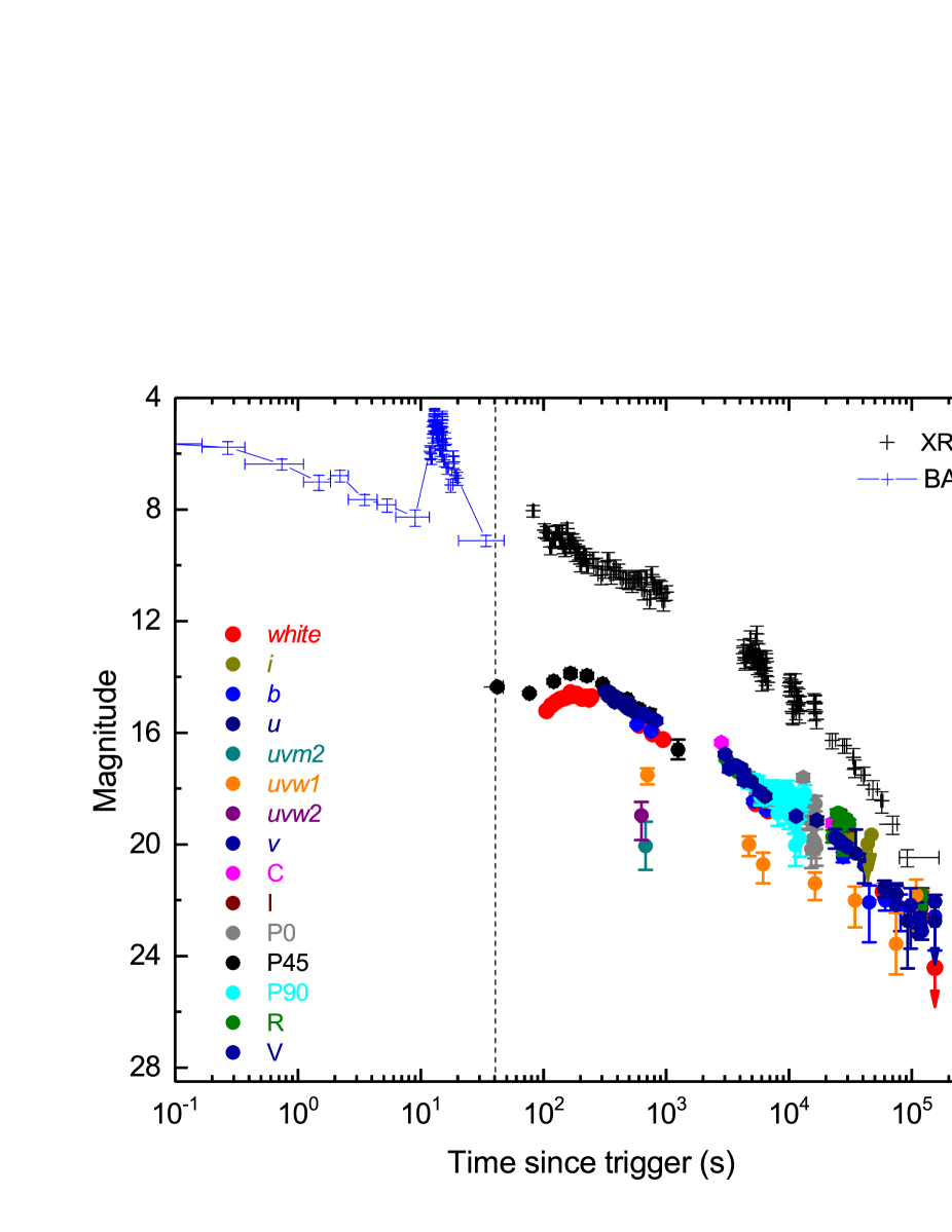
The observation log of GRB 140629A is given in Table 1 and the photometry for all filters and polarisations is presented in Table 8. All magnitudes are presented in Vega system except the GTC host galaxy observations, which are calibrated using the AB system. The final magnitude errors include the systematic error from the reference star calibration. The magnitudes in the table are not corrected for galactic extinction owing to the reddening of E(B-V) = 0.01 in the direction of the burst (Schlegel et al. 1998). For clarity, the afterglow light curves are shown in Figure 1.

Figure 1: X-ray and optical light curves for GRB 140629A. Observations from both BAT and XRT are given with blue crosses and black crosses, respectively. The BAT data are normalised to the same energy range as XRT. The optical data are shown with circles. The vertical dash line indicates the end of the prompt emission, given by $T_{90}$.

Table 1: Observation log of GRB 140629A.

$t_{start}$	$t_{end}$	Filters
MASTER
2014 Jun 29 14:18:03	Jun 29 21:58:09	C,V,R
$\it{Swift}$/UVOT
		white,u,v,b
2014 Jun 29 14:19:10	Jul 03 09:33:28	uvw1,uvw2
		uvm2
BOOTES
2014 Jun 29 22:19:47	Jun 30 03:47:33	i
OSN
2014 Jun 29 21:06:27	Jun 29 22:54:33	V,I,R
2014 Jun 30 22:20:55	Jul 01 00:19:09	V,I,R
2014 Jul 03 22:52:42	Jul 04 00:16:30	R
GTC
2015 Feb 27 06:03:20	Feb 27 06:23:50	u,g,r,i
2017 Feb 06 04:43:04	Feb 06 05:36:08	u,g,r,i
Spitzer
2015 Jun 05 16:48:20	Jun 05 19:00:48	3.6um

3.2 Temporal properties of the afterglow: An empirical fit

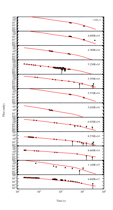
In this section, we fitted the light curves in X-ray and optical band with the empirical multi-segment smooth broken power law models  (Beuermann et al. 1999; Jóhannesson et al. 2006; Molinari et al. 2007).

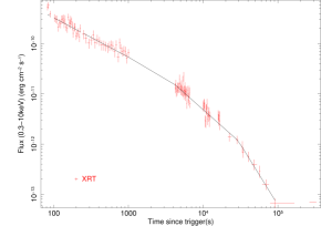
The X-ray light curve (0.3-10 keV) was obtained from the UK Swift Science Data Centre at the University of Leicester (Evans et al. 2009). As shown in Figure 2, the GRB 140629A X-ray light curve appears to show a canonical structure. An initial shallow decay is followed by a normal decay and then a steep decay (Zhang et al. 2006). To ensure two breaks are required, we first attempted to fit the light curve with a single broken power law. This resulted in a poor fit with a reduced chi square ($\chi^{2}$)$=1.32\leavevmode\nobreak\ (110\leavevmode\nobreak\ d.o.f.)$, and corresponding null hypothesis probability of only $0.01\%$. We then tested a smooth broken power law, which showed an improvement giving a reduced $\chi^{2}=1.10\leavevmode\nobreak\ (110\leavevmode\nobreak\ d.o.f.)$. For this model the best fitting parameters are $\alpha_{1}=0.84\pm 0.02$, $\alpha_{2}=1.87\pm 0.08$ with a break time $(8.8\pm 1.3)\times 10^{3}$ s. We then tried a smooth double broken power law model. This again improved the fit giving a reduced $\chi^{2}/d.o.f.$= 0.99/108. According to the Akaike information criterion (Akaike 1974; Liddle 2007, AIC), the smooth double broken power law model gives a lower AIC value in comparison to the smooth broken power law, suggesting the second break is required. This is also confirmed by the F-test, which suggests the second break is statistically required at more than 3$\sigma$ confidence. We can also check the need for an additional break using a Monte Carlo simulation. We create 10000 synthetic light curves by randomly selecting, for each data point of the observed light curve, a new flux and flux error using a Gaussian function for which the mean and standard deviation is equal to the original observed flux and flux error. Each of the synthetic light curves are then fitted with both a broken power law and a double broken power law. From the resulting distribution of the change in reduced $\chi^{2}$, we find that 98.2% of the simulated light curves have a change in reduced $\chi^{2}$ that is equal to or greater than that obtained for the observed X-ray light curve. The Monte Carlo simulation thus suggests that the double break power law is preferred over the broken power law model at the 2$\sigma$ confidence level. We do not identify any X-ray flares in the light curve.

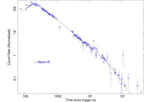
For the optical data, we normalised the observations in the different filters to Johnson-R band using the period between 3000 s and 30000 s, during which the light curves appear to decay in the same fashion (Oates et al. 2007). The resulting light curve is shown in Figure 2. We exclude data prior to 70 s from our analysis since the data are likely contaminated by the prompt emission. When fitting the optical data, we tested both a smooth double broken and a smooth triple broken power law against the data. The reduced $\chi^{2}$ changed from 1.53 (d.o.f = 123) to 1.38 (d.o.f=121) with the addition of third break. The smooth triple broken power law model is preferred according to F-test, which provides a chance probability of 0.0008. We also used the Monte Carlo method, which we used to determine the significance of improvement of an additional break in the X-ray light curve, on the optical data. The synthetic light curves in optical are fitted with both a double broken and a triple broken power law model. In the resulting distribution of the change in reduced $\chi^{2}$, we find that 99.9% of the simulated light curves have a change in reduced $\chi^{2}$ that is equal or greater than that obtained from the observed light curve. Thus the Monte Carlo simulation suggests the triple break power law is preferred over the double break power law at 3$\sigma$ confidence level. The values of the best fitting parameters for the optical and X-ray light curves are shown in Table 2 and the temporal fits are shown in Figure 2.

Figure 2: Fitting of the X-ray and optical GRB 140629A data. The normalised optical data are shown on the top panel with blue circles. The X-ray data are plotted on the bottom panel with red crosses. The black lines indicate the fitting results.

Table 2: Results of the best fit model to the X-ray and optical afterglows of GRB 140629A.

Optical		X-ray
Para	Value	Para	Value
$\alpha_{o,1}$	$-0.72^{+0.15}_{-0.33}$
$t_{o,b_{1}}$	$176.85^{+3.48}_{-3.22}$
$\alpha_{o,2}$	$0.91^{+0.03}_{-0.04}$	$\alpha_{x,1}$	$0.78^{+0.04}_{-0.04}$
$t_{o,b_{2}}$	$638.69^{+126.31}_{-105.89}$	$t_{x,b_{1}}$	$3428.52^{+1167.48}_{-808.52}$
$\alpha_{o,3}$	$1.17^{+0.01}_{-0.01}$	$\alpha_{x,2}$	$1.33^{+0.09}_{-0.07}$
$t_{o,b_{3}}$	$36164.96^{+7895.06}_{-5064.96}$	$t_{x,b_{2}}$	$31179.38^{+12470.62}_{-6560.38}$
$\alpha_{o,4}$	$1.97^{+0.18}_{-0.10}$	$\alpha_{x,3}$	$2.46^{+0.49}_{-0.24}$
$\chi^{2}/d.o.f.$	1.38/121	$\chi^{2}/d.o.f.$	0.99/108

3.3 Spectral analysis

3.3.1 Optical spectroscopy

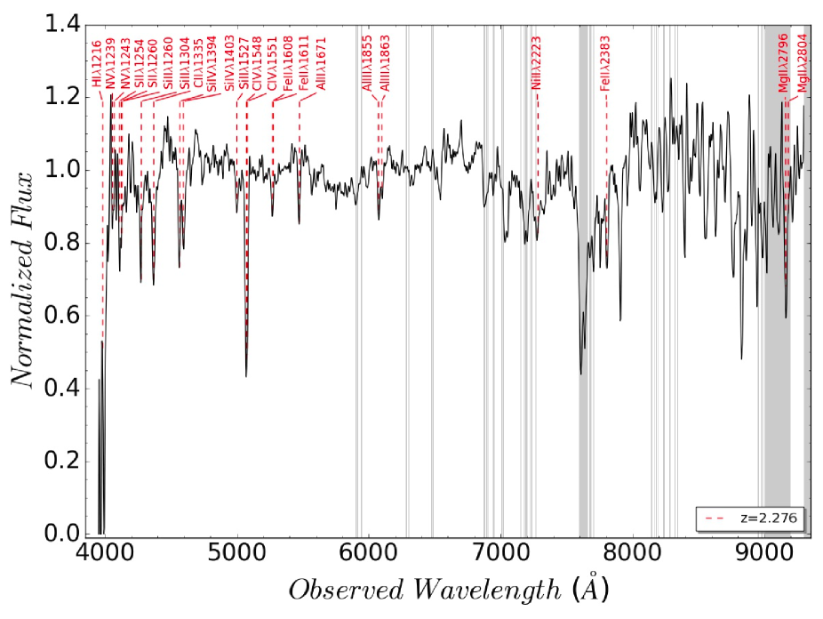
The optical spectrum observed by the 6 m BTA telescope, given in Figure 3, shows multiple absorption lines that we identify as Lyman-$\alpha$ (Ly-$\alpha$) absorption, Al III (1854.72Å, 1862.78Å), C IV (1548.20Å, 1550.77Å), C II (1334.53Å), N V (1238.81Å, 1242.80Å) Fe II (1608.45Å), Mg II (2803.53Å, 2796.35Å), Si ii (1260.42Å, 1304Å, 1526.72Å), Si IV (1393.76Å, 1402.77Å), and Al II (1670.79Å). All these absorption features can be attributed to a single intergalactic cloud at a common redshift z= 2.276 $\pm$0.001. This measurement is consistent with and refines previous determinations (Moskvitin et al. 2014; D’Avanzo et al. 2014; Xin et al. 2018) of the redshift of the GRB and its host galaxy. Both random and systematic errors are included in the uncertainty of the redshift. There are a few absorption features probably due to intervening systems in the line of sight, but we are not able to identify nor determine their redshift. In addition, we do not find any obvious strong emission lines in our spectrum. The absorption lines associated with the host galaxy at z=2.276 are identified on the spectrum provided in Fig 3.

We measured the equivalent widths (EW) of the detected absorption features (see Table 3). We found that the C IV line has a rest-frame EW value of 4.11$\AA$. This makes it the strongest absorption feature in the spectrum, confirming the identifications made by de Ugarte Postigo et al. (2012) and Xin et al. (2018). The EWs of the high ionisation species are higher than average, as compared to the results of de Ugarte Postigo et al. (2012), while the low ionisation species show no peculiarities. This implies the line of sight has a stronger ionisation absorption than is typically found for GRBs. We are also able to derive the EW ratio of ${C\textsc{IV}}/{C\textsc{II}}=2.72\pm 0.15$, which is consistent with the result of Xin et al. (2018), but higher than the median value found for GRBs in de Ugarte Postigo et al. (2012). We find the ratio of ${Al\textsc{III}}/{Al\textsc{II}}=1.44\pm 0.09$ and the ratio of ${Si\textsc{IV}}/{Si\textsc{II}}=5.1$, which are both higher than the median values found for GRBs de Ugarte Postigo et al. (2012). Using the ratios of ${C\textsc{IV}}/{C\textsc{II}}$ and ${Si\textsc{IV}}/{Si\textsc{II}}$, we find this GRB to be consistent with the highly ionised tail of the distribution of ionisation ratios of carbon and silicon; see Fig.11 in de Ugarte Postigo et al. (2012).

Figure 3: Overall view of the optical spectrum from BTA, obtained $\sim$4.1 hr after the GRB 140629A trigger. These metal lines of the absorption system in the GRB host galaxy are labelled in red, showing the corresponding transitions. The wavelength range with strong telluric absorption features are indicated by grey vertical lines.

Table 3: Spectroscopic information for the GRB 140629A.

Wave	Rest EW	Feature	$z$
(Å)	(Å)
4057.8	0.95 $\pm$ 0.12	N V$\lambda$1238.8	2.27553
4071.2	0.51 $\pm$ 0.07	N V$\lambda$1242.8	2.27581
4127.5	$<$ 0.48	S II$\lambda$1259.52 + Si II$\lambda$1260.42	–
4272.5	2.01 $\pm$ 0.11	O i$\lambda$1302.170 + Si II$\lambda$1304.4	–
4289.5	0.66 $\pm$ 0.06	Si II$\lambda$1309.3	2.27622
4374.9	1.51 $\pm$ 0.08	C II$\lambda$1334.5 + C II*$\lambda$1335.7	–
4584.6	2.96 $\pm$ 0.11	Si IV$\lambda$1393.8+1402.8	–
5007.2	0.58 $\pm$ 0.08	Si II$\lambda$1526.71	–
5077.4	4.11 $\pm$ 0.07	C IV$\lambda$1548.2+1550.8	–
5275.9	0.84 $\pm$ 0.06	Fe II$\lambda$1608.4+1611.2	–
5474.7	1.01 $\pm$ 0.05	Al II$\lambda$1670.8	2.27672
6085.6	1.45 $\pm$ 0.06	Al III$\lambda$1854.7+1862.8	–
7809.7	1.59 $\pm$ 0.16	Fe II$\lambda$2383.8	2.27616
9161.8	2.66 $\pm$ 0.13	Mg II$\lambda$2796.4+2803.5	–

3.3.2 Afterglow spectral analysis

As reported above, our temporal analysis of the X-ray light curve shows it to be best fit by a double broken power law that has two breaks at $\sim$3000 s and $\sim$30000 s. For each X-ray segment, we extracted an X-ray spectrum from the Swift/XRT GRB spectrum repository (Evans et al. 2009). We fit each spectra with a power law and two photoelectric absorption components: one for our Galaxy and the other for the host galaxy of the burst. The fitting results are shown in Table 4. The spectral indices of the three spectra are consistent with each other at 1$\sigma$ confidence. Therefore, the spectral slope does not show any evidence for evolution across the three X-ray light curve segments.

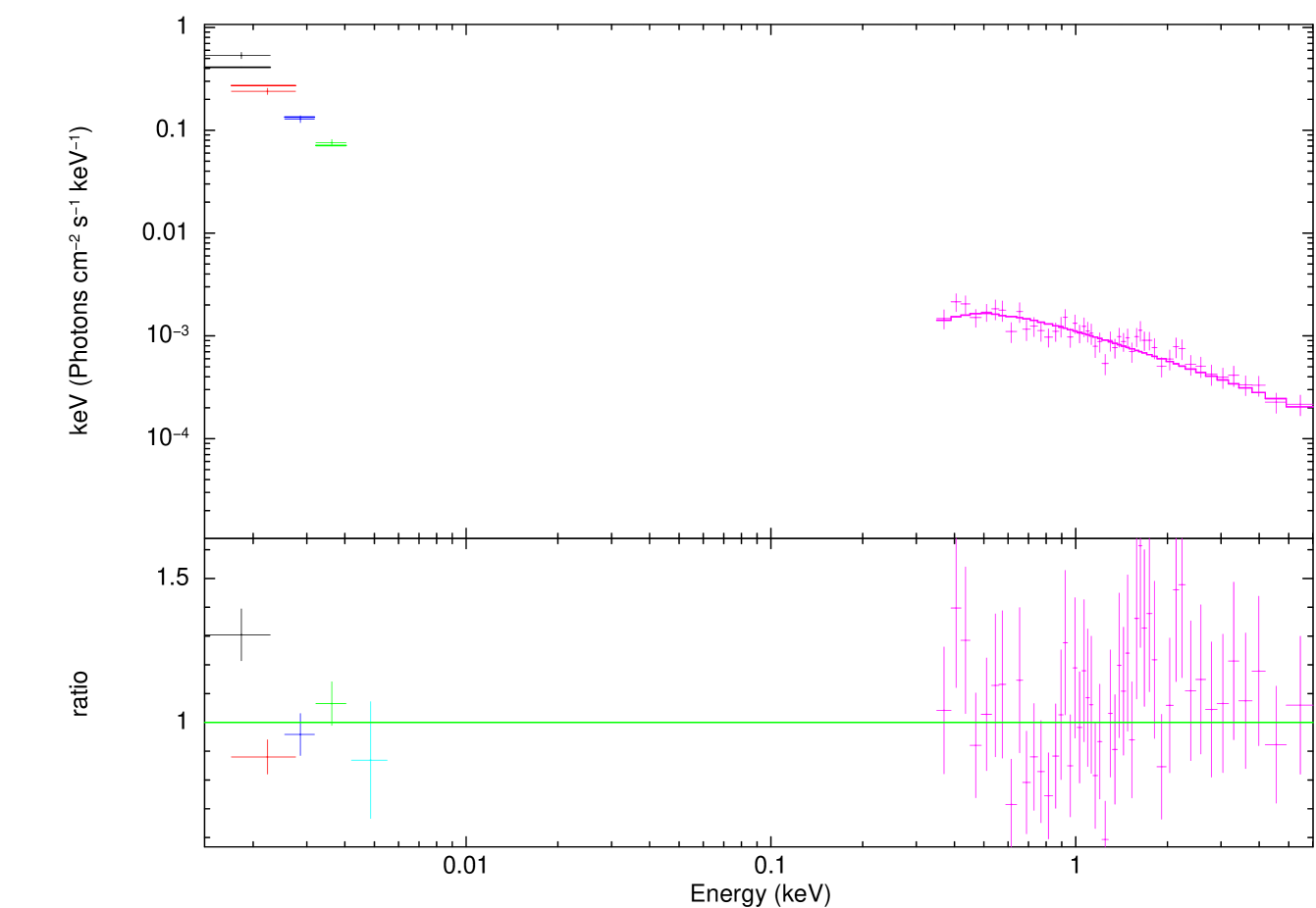
In order to constrain the spectral properties of the optical and the X-ray afterglow, we produced spectral energy distributions (SEDs) at $\sim$775 s and $\sim$9350 s after trigger, respectively. The joint SEDs (see Figure 4) were fit using Xspec 12.9.0 in the HEAsoft package (Arnaud 1996). We fit both a power law and a broken power law model to each of the SEDs, including components for dust and photoelectric absorption for both our Galaxy and the GRB host galaxy. We expect the synchrotron cooling frequency to be the cause of the spectral break in the broken power law model, therefore we fixed the difference in the two spectral indices to be $\Delta\beta=$0.5. For the extinction in our Galaxy, we fixed the dust component to have an $E_{B-V}=0.0067$ (Schlegel et al. 1998) and used the Milky Way (MW) extinction curve. We fixed the hydrogen column density of the MW to be 9.3$\times$ $10^{19}$cm^-2 (Kalberla et al. 2005; Osborne et al. 2014). The fitting results are listed in Table 5. We tested three extinction laws for the GRB host galaxy: $R_{V}$=3.08, $R_{V}$=2.93 and $R_{V}$=3.16 for the MW, Small Magellanic Cloud (SMC), and Large Magellanic Cloud (LMC), respectively.

In the SED obtained at 775s, we consider the power law to be the best model, since the F-test indicates that the broken power law model does not provide a significant improvement. Of the extinction models, the MW model provides the best chi-square of the three extinction models, but the reduced $\chi^{2}$ is similar for all three scenarios. For the SED at 9350s (see Fig 4), we find that the SMC model gives a better fit compared to the other two extinction models for both the power law and broken power law models. Again for this SED, the F-test indicates that the broken power law model does not improve the fit compared to the single power law model. The AIC supports this conclusion, as the AIC value increases for the broken power law model compared to the power law model. While there is no strong preference for a particular extinction law for the 775 s, the 9350 s SED clearly indicates the SMC extinction law is the best model. This is consistent with the preference for an SMC extinction law found for a large number of GRBs (Schady et al. 2010). We therefore assume this model during further investigation of this GRB. Comparing the SMC power law models of both SEDs, we find the parameters from the 775 s and 9350 s SEDs are consistent at 3$\sigma$ confidence level and that the $N_{H}$ values are consistent at 1$\sigma$ confidence with the best fit values determined from the X-ray spectrum.

Figure 4: Optical and X-ray SED in time interval of 9350s fitted with the SMCxBKP model.

Table 4: Spectral analysis of the X-ray light curve of the GRB 140629A afterglow fitted with three segments.

Segment	Time interval	Photon	$N_{H}$
	(s)	index	($10^{21}$cm-2)
1	$100-3\times 10^{3}$	$1.86_{-0.13}^{+0.14}$	$6.9_{-4.0}^{+4.4}$
2	$3\times 10^{3}-3\times 10^{4}$	$1.93_{-0.11}^{+0.11}$	$7.1_{-3.3}^{+3.6}$
3	$3\times 10^{4}-10^{5}$	$1.91_{-0.33}^{+0.36}$	$7.0_{-7.0}^{+12.5}$

Table 5: Fit results for the GRB 140629A afterglow SEDs.

Model	R-chi.	$E_{B-V}$	$N_{H}$	Photon
	/D.O.F	(mag)	($10^{21}$cm-2)	index
775s
MW$\times$POW	0.94/27	$0.131^{+0.017}_{-0.017}$	$3.30^{+2.24}_{-2.02}$	$1.948^{+0.026}_{-0.026}$
LMC$\times$POW	1.02/27	$0.108^{+0.013}_{-0.013}$	$3.69^{+2.27}_{-2.04}$	$1.963^{+0.027}_{-0.027}$
SMC$\times$POW	1.05/27	$0.085^{+0.011}_{-0.011}$	$3.40^{+2.24}_{-2.02}$	$1.952^{+0.025}_{-0.026}$
MW$\times$BKP	0.94/26	$0.160^{+0.006}_{-0.006}$	$6.23^{+2.13}_{-1.90}$	$1.563^{+0.010}_{-0.010}$
LMC$\times$BKP	0.99/26	$0.125^{+0.005}_{-0.005}$	$4.67^{+2.05}_{-1.84}$	$1.502^{+0.010}_{-0.010}$
SMC$\times$BKP	1.02/26	$0.098^{+0.004}_{-0.004}$	$4.35^{+2.04}_{-1.83}$	$1.489^{+0.010}_{-0.010}$
9350s
MW$\times$POW	1.92/50	$0.135^{+0.017}_{-0.017}$	$6.52^{+2.01}_{-1.86}$	$2.020^{+0.024}_{-0.024}$
LMC$\times$POW	1.44/50	$0.122^{+0.013}_{-0.013}$	$7.51^{+2.05}_{-1.89}$	$2.052^{+0.023}_{-0.023}$
SMC$\times$POW	1.25/50	$0.083^{+0.010}_{-0.009}$	$7.20^{+2.01}_{-1.85}$	$2.039^{+0.020}_{-0.020}$
MW$\times$BKP	1.95/49	$0.135^{+0.017}_{-0.017}$	$6.52^{+2.01}_{-1.86}$	$2.020^{+0.024}_{-0.024}$
LMC$\times$BKP	1.47/49	$0.122^{+0.013}_{-0.013}$	$7.51^{+2.05}_{-1.89}$	$2.053^{+0.023}_{-0.023}$
SMC$\times$BKP	1.28/49	$0.085^{+0.010}_{-0.009}$	$7.16^{+2.01}_{-1.85}$	$2.040^{+0.020}_{-0.020}$

3.4 Host galaxy SED fitting

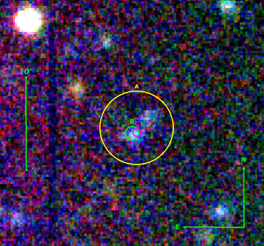
In order to study the GRB host galaxy, late time observations were taken by 10.4 m GTC at two separate epochs. An object was found within the XRT and UVOT error circles in the second epoch, 2.7 yr after the trigger (as shown in Figure 5). Spitzer also observed the field $\sim 1$ yr after the burst in the infrared in the 3.6 $\mu m$ band. By this time, the afterglow contribution is negligible.

The brightness of the host galaxy is 24.94$\pm$0.24 mag in Sloan-r band, which is within the brightness distribution for GRB host galaxies (see Fig. 2. in Guziy et al. (2005)). It is slightly fainter than the reference $M^{\star}_{r}$ galaxy at the same distance, where $M^{\star}_{r}$ is the r-band absolute magnitude, considering $M^{\star}_{r}$=-20.29+5log$(H_{0}/100)$ (Lin et al. 1996) and adopting an Einstein-de Sitter Universe model where the spectrum of the $M^{\star}_{r}$ galaxy was assumed to be a power law with an index of 2.

Figure 5: Sloan gri-bands false colour image of the field of GRB 140629A taken with the 10.4 m GTC on July 2, 2017. Circle A (yellow dash circle) represents the 4 arcsec radius error circle of the XRT. The circle B (green circle) and C (pink circle) represent the UVOT observation in 0.74 arcsec and 0.42 arcsec, respectively (Lien et al. 2014; Breeveld & Lien 2014). The host galaxy is clearly found at the burst location. North is up and east to the left.

Figure 6: GRB 140629A host galaxy observations overlaid with the best fit host galaxy template.

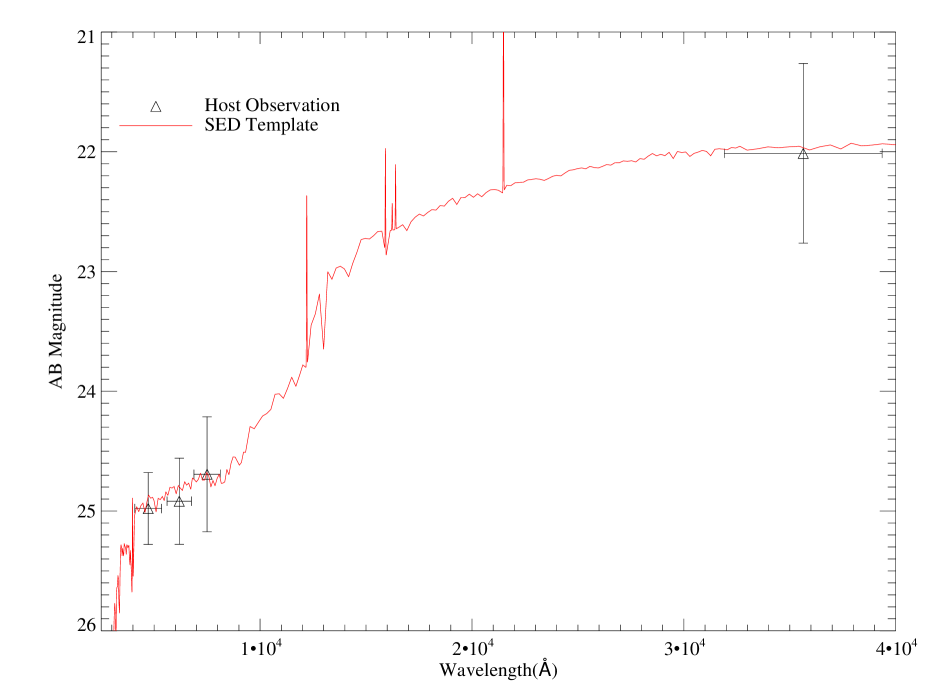
The four photometric magnitudes for the host galaxy were fit with a set of galaxy templates based on the models from  Bruzual & Charlot (2003) at a fixed redshift  (Castro-Tirado et al. 2007; Krühler et al. 2011) using the LePhare package (v.2.2;  Arnouts et al. 1999; Ilbert et al. 2006). As shown in Figure 6, the optical SED is reproduced best (reduced $\chi^{2}$/dof=0.1/3) by a template of a galaxy with a starburst age of $1.14_{-0.35}^{+1.03}$ Gyr and a mass of log($M_{*}/M_{\odot}$)=$8.3_{-0.4}^{+0.9}$ , which is lower but consistent within errors with $10^{9.3}M_{\odot}$, i.e. the average value of GRB hosts (Savaglio et al. 2009). The absolute bolometric magnitude of the host galaxy is -22.49 mag and the star formation rate (SFR) is log(SFR)=$1.1_{-0.4}^{+0.9}$ M_⊙ yr^-1, which is determined from the UV luminosity of the rest-frame SED (Kennicutt 1998). The specific star formation rate (SSFR) for this burst is log(SSFR)=$-7.5_{-1.3}^{+0.6}$ yr^-1.

3.5 Polarisation

According to our observations with the MASTER network, GRB 140629A reached maximum optical brightness $\sim$150 s after the burst with 13.8 mag in white light, measured using the polariser, after which it decays as a power law. The difference between the signals obtained in the two polarisers for the time interval from 4463 s to 11596 s were computed as $Q=\frac{I_{1}-I_{2}}{I_{1}+I_{2}}$. It was found that the dimensionless time-averaged Stokes parameter is $Q=2.5\pm 2.6\%$. For the derived uncertainty of 2.6%, the 1$\sigma$ upper limit for the degree of linear polarisation P is about 18% (see Fig. 14 of Gorbovskoy et al. (2012): the value of P = 18% matches 1$\sigma$ probability $L=100\%-68\%=32\%$ for the curve corresponding to a relative accuracy 2.6%). At the same time, a non-evolving, weak polarisation result was obtained by Hiroshima one-shot wide-field polarimeter(HOWPol) at the Kanata telescope. They found P $\sim 2\%$ between $\sim 70$ to $\sim 1200$ s in the burst frame (Fig.10 in  Gorbovskoy et al. (2016)). Our upper limit is consistent with their result.

4 Discussion

We have studied the optical and X-ray afterglow of GRB 140629A. There is no strong evidence for spectral evolution, with the spectral indices consistent within $3\sigma$. The optical light curve begins with an initial rise, which decays thereafter with two breaks. The X-ray light curve decays from the start of observations and also decays with two breaks. A weak polarisation signal was found in the afterglow observations and we were able to obtain information on the host by fitting the host galaxy SED. In the following subsections, we examine the closure relations between the temporal and spectral indices. Then we use the data to test the jet structure to determine a plausible scenario to explain this burst. Finally, we explore the properties of the host.

4.1 Closure relationship in optical and X-ray data

The closure relations are a set of equations that relate observational parameters, namely the spectral and temporal indices, with the microphysical parameters, for example $p$ (the electron energy spectral index), $\upsilon_{m}$ (the characteristic synchrotron frequency of the electrons at the minimum injection energy) and $\upsilon_{c}$ (the cooling frequency). Typically, the closure relations are used to determine the location of the observing bands relative to the synchrotron frequencies, $\upsilon_{m}$ and $\upsilon_{c}$, and also the environment in which the burst occurs (Sari et al. 1998; Sari & Piran 1999; Piran 2004; Zhang & Mészáros 2004; Zhang et al. 2006).

For GRB 140629A, we examined the three segments of the X-ray light curve. Spectral evolution is not observed across these segments. We first examined the second segment since this is expected to be consistent with the normal decay phase. After the first break at $\sim 3000$ s, the light curve becomes steeper with $\alpha_{x,2}=1.33^{+0.09}_{-0.07}$. This slope is typical of the normal decay phase ($\sim$1.1-1.5; Zhang et al. (2006)). The spectral slope for this segment is $\beta_{X,2}=0.93^{+0.11}_{-0.11}$. During this phase, the temporal index and spectral index are consistent with the closure relation $\alpha=3\beta/2$, which is for electrons that are slow cooling within the range $\upsilon_{m}<\upsilon_{x}<\upsilon_{c}$ without energy injection in a uniform circumstellar medium. The first segment decays with $\alpha_{x,1}=0.78^{+0.04}_{-0.04}$ until 3430 s and the spectral index is $\beta_{X,1}=0.86^{+0.14}_{-0.13}$. We first tested a simple non-injected model and found that neither $\alpha=3\beta/2$, $\alpha=(3\beta+1)/2$ and $\alpha=(1-\beta)/2$ agree with the theoretic prediction (¿3 $\sigma$). Only the relation $\alpha=(3\beta-1)/2$ in the $\upsilon_{x}>\upsilon_{c}$ case can fit the indices at  1$\sigma$. However, comparing the best fit closure relations between the first and second segments implies there must be a spectral break between the two segments which is not observed. We therefore examined more complex closure relations that include energy injection. It is assumed that the luminosity evolves as $L(t)=L_{0}(t/t_{b})^{-q}$, where $q$ is the luminosity index affected by the energy injection (Zhang et al. 2006). The relation satisfied is $\alpha=(q-1)+(2+q)\beta/2$. This is for a constant density medium with slow cooling electrons, where $\upsilon_{m}<\upsilon_{x}<\upsilon_{c}$. This relation requires $q=0.59\pm 0.05$. This relation can also be used in the case $\upsilon<\upsilon_{m}$, but we can able to rule this out since the observed slope is 3$\sigma$ away from the predicted slope. Therefore, the change between the first two segments most likely signals the end of additional energy injection, after which the afterglow enters the normal decay phase. The origin of the shallow decay phase (plateau) is also an issue that has been debated. The plateau may be categorised as having an internal or external origin, depending on the behaviour of the temporal index of the next light curve segment. The internal plateau is followed by a steep decay whose index is larger than 3, even as large as 10. This plateau is a result of the internal dissipation of a millisecond magnetar as it spins down (Liang et al. 2007; Troja et al. 2007; Yi et al. 2014). In this case when the energy injection ceases a sharp drop in the light curve is observed. The decay index following an external origin for the plateau is typically smaller than 3 and is well explained by energy injection into the external shocks from either slower travelling shells that are received later or by a long-lived central engine (Dai & Lu 1998; Zhang & Mészáros 2001; Tang et al. 2019). For GRB 140629A, the plateau is followed by a normal decay with a slope of 1.33, indicating that it has an external origin. The change in slope across the second break at $\sim$30000s is $\Delta\alpha\sim 1.1$. We immediately ruled out several potential interpretations for this break, including the transition of the cooling frequency across the band that predicts a $\Delta\alpha\sim 0.25$ (Sari et al. 1998); an energy injection from refreshed shocks; a long-lasting central engine that predicts a $\Delta\alpha\sim 0.7$ (Rees & Mészáros 1998; Sari & Mészáros 2000; Zhang & Mészáros 2002), or an external density change, which in order to achieve such a large change in alpha, the density would have to decrease by a factor larger than $10^{3}$ (Nakar & Granot 2007; Fong et al. 2012). Therefore, this observed break can only be explained by the jet geometry, for example a jet break. The light curve after the jet break should follow $\varpropto t^{-p}$. For the third segment, the best fitting closure relation is for a spreading jet with slow cooling, where $\upsilon_{m}<\upsilon_{x}<\upsilon_{c}$ is consistent with the previous segments. Using the spectral index for X-ray segment 3, we found a temporal slope of $-2.82\pm 0.35$, which is consistent with the observed temporal slope at 1.1 sigma.

For the optical afterglow, we excluded data before 70 s from the fitting process as they were observed during the prompt emission phase and thus may be dominated by the tail of the prompt emission. The best fit to the rest of the optical data required four segments. The first segment is an initial rise that peaks at 180 s. This is likely to be the onset of the afterglow and is discussed in more detail in Sec 4.4. In that section we focus on the decay segments. After the peak, a slope of $\alpha_{o,2}=0.91^{+0.03}_{-0.04}$ can be explained by the scenario of energy injection in a slow cooling interstellar medium (ISM) model with $\upsilon_{m}<\upsilon_{o}<\upsilon_{c}$. We obtained a value of $q=0.73\pm 0.04$, which is consistent with that derived from the X-ray energy injected decay segment at 2$\sigma$ confidence level. Furthermore, the next segment with a temporal index of $\alpha_{o,3}=1.17^{+0.01}_{-0.01}$ is in agreement with the $\alpha=3\beta/2$ at 3$\sigma$ confidence level, which also suggests that the afterglow ceases to be energy injected and enters the normal decay phase in which electrons are slow cooling in uniform medium. Other explanations are ruled out because the temporal indices derived using the spectral indices and the other closure relations are inconsistent with the measured values at ¿3$\sigma$. The last optical decay segment breaks to a steeper decay at a time ($\sim$30000s) consistent, at 1$\sigma$, with the jet break in the X-ray light curve. The optical decay slope for this segment is shallower than $-2.82\pm{0.35}$ derived using the X-ray spectral index, but is consistent within 3$\sigma$ confidence level. As the jet break is a geometric effect, it should have an achromatic break time and the same post-break decay index at all frequencies. For GRB 140629A, the break is achromatic in time, but the slopes of the post-break power law components are only marginally consistent; the decay index of the X-ray light curve is steeper than that in the optical. This has also been found for other GRBs such as GRB 050730 and GRB 051109A (Panaitescu 2007).

Overall, our analysis of the optical and X-ray light curves draws a consistent picture. The light curves are both produced by the blast wave jet impinging on the constant density circumstellar medium in the slow cooling regime, where $\upsilon_{m}<\upsilon_{o}<\upsilon_{x}<\upsilon_{c}$. A long-lasting central engine is still active after the prompt emission has vanished, which when it ceases, causes the light curve to enter the normal decay phase. At $\sim$30000 s, an achromatic break is observed in the optical and X-ray light curves, which can be attributed to the jet break. The same process in both bands supports the X-ray radiation and the optical radiation originating from a single component outflow.

4.2 Physical model

Following  Zhang et al. (2015), we fitted the multiwavelength data with a model based on numerical simulations to obtain further information about the jet. This process is based on a 2D relativistic hydrodynamics (RHD) simulation, which assumes a jet with a top-hat Blandford-McKee profile (Blandford & McKee 1976) that decelerates into a constant density medium. An ISM-type medium can be assumed as it has been found to explain the observations of most GRB afterglows (Panaitescu & Kumar 2001; Racusin et al. 2009; Schulze et al. 2011) and is consistent with our analysis of GRB 140629A, as discussed in the previous section. Other assumptions of the model include that the radiation and dynamics of the collimated relativistic blast wave are assumed to be separate, and that the fraction of energy contained within the magnetic field at the front of the blast wave is low. The RHD simulation is performed with a relativistic adaptive mesh that employs a high-resolution adaptive mesh refinement (AMR) algorithm (Zhang & MacFadyen 2006). This algorithm calculates the radiation transfer at a given observer time, angle, and distance along a line of sight (van Eerten et al. 2012; van Eerten & MacFadyen 2013). The numerical model takes into account all the factors that can affect the shape of a jet break: (i) lateral expansion, (ii) edge effects, and (iii) off-axis effects. By fitting such a model to the optical and X-ray light curves, we are able to constrain some key physical parameters of the jet.

Because the data before the onset of the afterglow are still dominated by the prompt emission, we only model the data after 180 s. We corrected the optical data for extinction from the MW (Schlafly & Finkbeiner 2011; Schlegel et al. 1998) and the host galaxy, assuming the best fit host extinction law from the SED fitting (SMC) (for details see the previous section, Pei 1992; Schady et al. 2007, 2010). We then converted the extinction corrected light curves to flux density at the central wavelength of the corresponding filter. For the X-ray light curve, the galactic and host neutral hydrogen absorption was also corrected to get the intrinsic flux density at 1 keV.

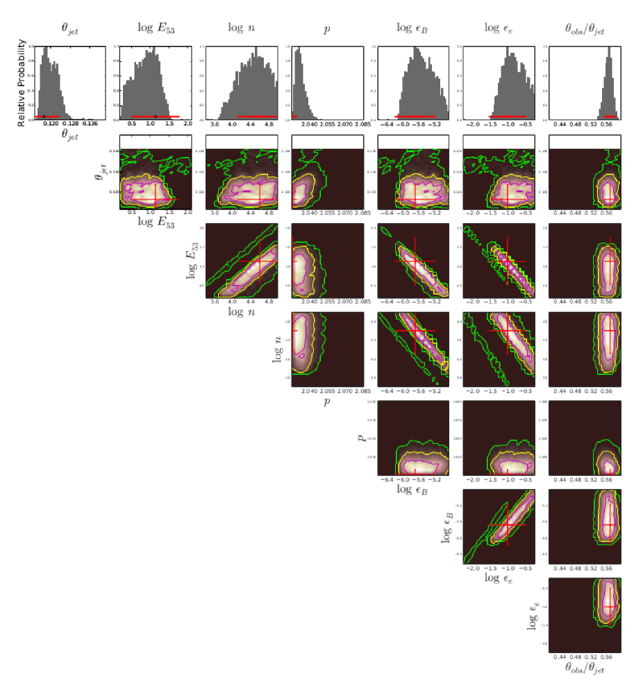
The numerical modelling calculates the flux density at any frequency and observer time. The Markov Chain Monte Carlo method is used to determine the best parameter values (i.e. the smallest $\chi^{2}$ value) (Laskar et al. 2016; Sánchez-Ramírez et al. 2017). The parameters determined include the total energy $E_{tot,iso,53}$, the fraction of shock energy given to the electrons $\epsilon_{e}$, the fraction of shock energy given to the magnetic fields $\epsilon_{B}$, the density of the medium $n$, the electron energy index $p$, the jet opening angle $\theta_{jet}$ and the observed angle $\theta_{obs}$. The starting ranges for each parameter are $\theta_{jet}\in$ [0.045,0.5], $E_{tot,iso,53}\in$ [$10^{-10}$,$10^{3}$], $n\in$ [$10^{-5}$,$10^{5}$], $p\in[2,4]$, $\epsilon_{B}\in$ [$10^{-10}$,1], $\epsilon_{e}\in$ [$10^{-10}$,1], and $\theta_{obs}$/$\theta_{jet}\in$ [0,1]. For more details, see Zhang et al. (2015).

Table 6: Best fit parameters of the numerical simulation to the multiwavelength afterglow.

Modelling fitting
Parameters	Value	Err (-)	Err (+)
$\theta_{jet}$	0.1171	0.0002	0.0061
$\log\,E_{tot,iso,53}$	1.1414	0.6226	0.0675
$\log\,n$	4.6106	0.5047	0.1875
$p$	2.0263	0.0008	0.0039
$\log\,\epsilon_{B}$	-5.6730	0.1616	0.5201
$\log\,\epsilon_{e}$	-0.9974	0.1347	0.5294
$\theta_{obs}$/$\theta_{jet}$	0.5713	0.0163	0.0048

With these settings, the resulting best fit parameters and their uncertainties are listed in Table 6. The uncertainty on the parameters are calculated at the $68\%$ confidence level in the local mode region. The best fit to each light curve for the different wavelengths is shown in Figure 7 and the parameter distribution is given in Figure 13. In this case, the numerical model finds a solution with best fit parameters of $\theta_{jet}\sim 6.7^{\circ}$ and $\theta_{obs}\sim 3.8^{\circ}$, giving a total energy release of $1.4\times 10^{54}$erg. Since the modelling focusses on the effects of the jet break and based on a 2D RHD simulation, the energy injection is not taken into account, but the fit can still roughly describe most of the data. Furthermore the analytic approach ($p=2.8\pm 0.3$) and the simulation both have $p$ values that agree at 3$\sigma$. We find the opening angle to be typical of GRBs (Zhang et al. 2015; Racusin et al. 2009). The relative off-axis angle, $\theta_{obs}/\theta_{jet}=0.57$, is also consistent with the distribution, which peaks at 0.8, given in Zhang et al. (2015). We also obtained a high circumstellar density value that suggests this burst originated in a dense environment. In addition, our value for $\log\,\epsilon_{B}\sim$-5.7 is consistent with the modelling result from (Xin et al. 2018).

Figure 7: Best fit model determined from the numerical simulations overlaid on the observations at different wavelengths. The corresponding frequency is shown on the right corner in each panel in unit of Hz. The x-axis is the time since trigger in units of seconds. The observed flux density of each instrument is indicated on the y-axis in units of mJy. All data were corrected for MW and host galaxy absorption and extinction effects before modelling. Red solid lines represent the modelled light curves.

4.3 Jet angle and empirical relation

The $E_{r,iso}$ is the energy in $\gamma$-rays calculated assuming that the emission is isotropic. The collimation corrected energy is calculated following

$$E_{\gamma} = E_{\gamma,\rm iso}f_{\rm b}=E_{\gamma,\rm iso}\left(1-\cos\theta_{\rm j}\right),$$ (1)

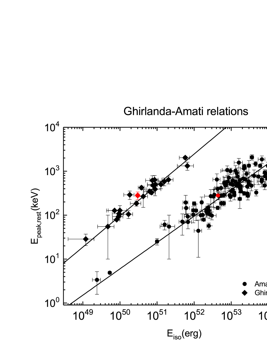
where $f_{\rm b}$ is the collimation correction factor. For GRB 140629A, from the high-energy emission, we determined the isotropic rest-frame energy to be $E_{\gamma,\rm iso}=4.4\times 10^{52}$ erg and the observed $E_{peak}$= $86\pm 17$ keV. The peak of the energy spectrum in the rest frame is $E_{p,rest}$=$E_{peak}\times(1+z)$= $281\pm 55$ keV. The $E_{\gamma,\rm iso}$ and $E_{p,rest}$ of this burst lie within the distribution of Amati correlation as shown in Figure 8 (Amati et al. 2002, 2008, 2009; Nava et al. 2012).

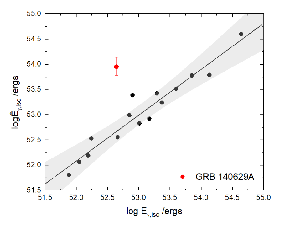
From the numerical modelling, we obtained a jet opening angle, $\theta_{jet}=6.7^{\circ}$. The collimation corrected energy is $E_{\gamma}=3.0(\pm 0.3)\times 10^{50}$erg. Together with $E_{p,rest}$, this burst is also consistent with the Ghirlanda relation (Ghirlanda et al. 2004, 2007) also shown in Figure 8. GRB 140629A is denoted with a red point on both these empirical relations. The bootstrap method is used to estimate their errors. We also tested the relation between $E_{\gamma,\rm iso}$, $E_{p,rest}$ and $t_{b,rest}$ (the jet break time) known as Liang-Zhang relation (Liang & Zhang 2005), but GRB 140629A is inconsistent with this correlation, shown in Figure 9. It is unclear why this GRB appears to be an outlier of the Liang-Zhang relation; it could be due to selection effects relating to the GRB prompt emission.

Figure 8: Location of GRB 140629A (red point) with the Ghirlanda (black prism) and Amati relation (black circle) derived from other typical GRBs (data from Ghirlanda et al. 2007; Amati et al. 2008, 2009). The two straight lines indicate the two empirical relations.

Figure 9: Location of GRB 140629A (red point) with the Liang-Zhang relation (black circle) derived from other typical GRBs (data from Liang & Zhang 2005). $\hat{\rm{E}}_{\gamma,iso}$ represents the calculated energy with the Liang-Zhang relation. The straight line indicates the empirical relations and the grey zone corresponds to the 3$\sigma$ confidence level.

4.4 Early optical rise

Both MASTER and UVOT observed a peak at $\sim$180 s (see Figure 1). There are several explanations for this rise based on physical mechanisms and geometric scenarios, which include the passage of the peak synchrotron frequency through the observing band, the reverse shock, decreasing extinction with time, an off-axis jet, two component outflows, and the onset of the forward shock in the case of an isotropic outflow (Oates et al. (2009)). We discuss each of these options in turn.

The peak synchrotron frequency of the forward shock $\nu_{m,f}$ is expected to cross from blue to red frequencies, producing a chromatic peak which evolves at $t^{2/3}$. If the peak were due to the crossing of $\nu_{m,f}$ across the optical bands, the spectrum after peak is expected to be consistent with $\nu^{-(p-1)/2}$ for $\nu_{m}<\nu<\nu_{c}$ (Sari et al. 1998). The effective frequency of the MASTER clear filter and the UVOT white filter are $5746\AA$ and $3469\AA$ respectively (Poole et al. 2008; Kornilov et al. 2012), thus the MASTER clear filter is the redder filter. Using the central wavelengths of the white and clear filters converted to frequency and assuming $p$=2, we predicted the peak in the bluer filter should appear 54 s earlier than the peak in the redder filter. We therefore selected the optical data from the MASTER clear filter and UVOT white filter between 90 s and 600 s and fit with a smooth broken power law model. The results are shown in Table 7. The measured difference between the peak times of the two filters is only 9 s and are the same within a 1$\sigma$ confidence level. This is inconsistent with the predicted peak time difference by 4$\sigma$. This therefore makes it unlikely that the passage of $\nu_{m,f}$ is the cause of the peak in the optical filters.

Table 7: Fitting result from the first optical bump in two filters.

Ins.	Slope1	Peak time	Slope2
MASTER	$-0.87_{-0.15}^{+0.16}$	$170.0_{-11.8}^{+13.6}$	$1.09_{-0.13}^{+0.12}$
UVOT	$-1.01_{-0.10}^{+0.10}$	$179.9_{-3.0}^{+3.4}$	$0.94_{-0.02}^{+0.03}$

For the reverse shock model, we just considered the constant density medium as this is consistent with the results of Section 4.1. In this case, when the peak synchrotron frequency of the reverse shock $\nu_{m,r}$ is lower than the optical wavelength, $\nu_{m,r}<\nu_{opt}$, the light curve is expected to decay after the peak with $\alpha=(3p+1)/4$ (Zhang et al. 2003) with $p\sim 2$ in this case, $\alpha\sim-1.75$. On the contrary, if $\nu_{m,r}>\nu_{opt}$, then the temporal index after the peak should be $\alpha\sim-0.5,$ which is followed by a decay of $\alpha=(3p+1)/4$. The slope after the early optical peak is inconsistent (¿3$\sigma$ confidence) with both these scenarios for GRB 140629A.

Another option to produce the rise could be dust destruction. An initially high level of dust could cause optical extinction, as this dust is destroyed by the radiation from the GRB, a chromatic peak is produced with different rise indices for the different filters (Klotz et al. 2008). As dust affects the bluest filters more strongly, the redder filters rise less steeply compared to the blue filters. While the redder MASTER filter has a shallower rise compared to the bluer UVOT filter, the slopes are consistent within 1$\sigma$ and we do not consider this to be a likely cause of the optical rise.

In the forward shock model, a peak is observed when the jet ploughs into the external medium. It is expected to produce an achromatic rise with $\alpha\sim 1$ in the thick shell case with a constant density medium (Sari & Piran 1999; Granot et al. 2002). This is consistent with the rising slopes given in Table 6. We can exclude more complex jet geometry such as off-axis viewing and two component outflows. If the observer’s viewing angle is larger than the half-opening angle of the jet a rise is produced when the Lorentz factor $\varGamma$ decrease to $(\theta_{obs}-\theta)^{-1}$ (Granot et al. 2002, 2005). However, the modelling result shows that the observer angle is smaller than the half-opening angle, thus this explanation can be excluded. Also the two-component outflow can be ruled out because we find that the afterglow can be explained by a single component outflow in Sec 4.1. Thus, the achromatic peak and consistent slope make the forward shock the most likely option for GRB 140629A early optical bump.

4.5 Initial bulk Lorentz factor

The initial Lorentz factor ($\varGamma_{0}$) is an important parameter describing the initial parameters of the jet. A common way to estimate the initial Lorentz factor is to use the peak time of the early afterglow light curve. The peak time determines the deceleration time of the external forward shock and occurs when roughly half of the blast wave jet energy is transferred to the surrounding medium, as predicted in the blast wave jet model (Sari et al. 1999; Kobayashi & Zhang 2007). At this point, the Lorentz factor is half that of the $\varGamma_{0}$. For a constant density medium, the initial Lorentz factor can be expressed as

$$\varGamma_{\rm 0}=2.0\left[\frac{3E_{\rm\gamma,iso}(1+z)^{3}}{32{\pi}nm_{\rm p}c^{5}{\eta_{\gamma}}t_{\rm p}^{3}}\right]^{1/8},$$ (2)

where $z$ is the redshift, $n$ is the density of the external medium, $m_{p}$ is the proton mass, $c$ is the speed of light, $\eta_{\gamma}$ is the radiation efficiency, and $t_{p}$ is the peak time of the afterglow onset bump (Sari et al. 1999; Liang et al. 2010). In the optical data, we found the early onset bump peaks at $\sim$180 s after trigger. Using the parameters, $n$ and $\eta_{\gamma}$, obtained from the modelling, the initial Lorentz factor for GRB 140629A is $\varGamma_{0}=118\pm 5$. Lü et al. (2012) corrected the coefficient to 1.4 by integration of blastwave dynamics before the deceleration time. Using the revised equation, we obtained a Lorentz factor of $\varGamma_{0}=82\pm 4$, which is lower than the value of 315 obtained by (Xin et al. 2018). We likely got such different results because the parameters $\eta_{\gamma}$ and $n$ obtained from our modelling are one or two magnitudes higher than those used by Xin et al. (2018). For GRB 140629A, the radiative efficiency, defined as $\eta_{\gamma}$=$E_{\rm\gamma,iso}$/$(E_{\rm\gamma,iso}$+$E_{\rm K,iso})$=$E_{\rm\gamma,iso}$/$E_{tot,iso}$, is 3.1%; this is within the radiative efficiency distribution for long GRBs (see figure 10 in Racusin et al. 2011).

4.6 Properties of the optical polarisation

The optical polarisation of GRBs provides additional clues to determine the structure and radiation mechanisms of the jet (Covino et al. 2004; Granot & Ramirez-Ruiz 2010). Most GRB polarisation observations have been taken during the afterglow as the prompt emission is short lived. Both linear and circular polarisations have been found at optical wavelengths (Covino et al. 1999; Wiersema et al. 2014). In our observation of 140629A, we find an upper limit of $P<18\%$, which is consistent with the result from HOWPol (Gorbovskoy et al. 2016). Such a low degree of linear polarisation implies this burst is weakly polarised. This is considered to be confirmation that the dominant afterglow emission mechanism is synchrotron radiation. Moreover, the polarisation measurement suggests an average dust-to-gas ratio in the GRB host galaxy along the line of sight lower than our Galaxy (Klose et al. 2004), which is consistent with our findings in Section 4.7. It has been proposed that the polarisation light curves have varied trends for various jet structures, especially at the jet break time (Rossi et al. 2004; Granot & Ramirez-Ruiz 2010). However, our polarisation observations were taken before the jet break and therefore we cannot use them to constrain the jet models for this burst.

4.7 Properties of the host galaxy and environment

The optical to X-ray SED at 9350 s gives the $N_{H}$ along the line of sight as 7.2$\times 10^{21}$cm^-2, which is higher than that of our Galaxy ($N_{H}^{MW}$=9.3$\times$ $10^{19}$cm^-2 ) by two orders of magnitude. In addition, the intrinsic $E_{B-V}$ is 0.083 $\pm$ 0.009, which is also one order of magnitude higher than that of our Galaxy. Therefore, the dust-gas ratio along the line of sight to GRB 140629A is $N_{H}/A_{V}=2.96\times 10^{22}$cm^-2. This is lower than that of our Galaxy by one order of magnitude and is slightly lower than the mean value of $3.3\times 10^{22}$cm^-2 for the SMC extinction model from Schady et al. 2010. This burst does not show any distinct feature in comparison with the other typical GRBs in the $N_{H}-A_{V}$ plane (see Figure 9 in Littlejohns et al. 2015).

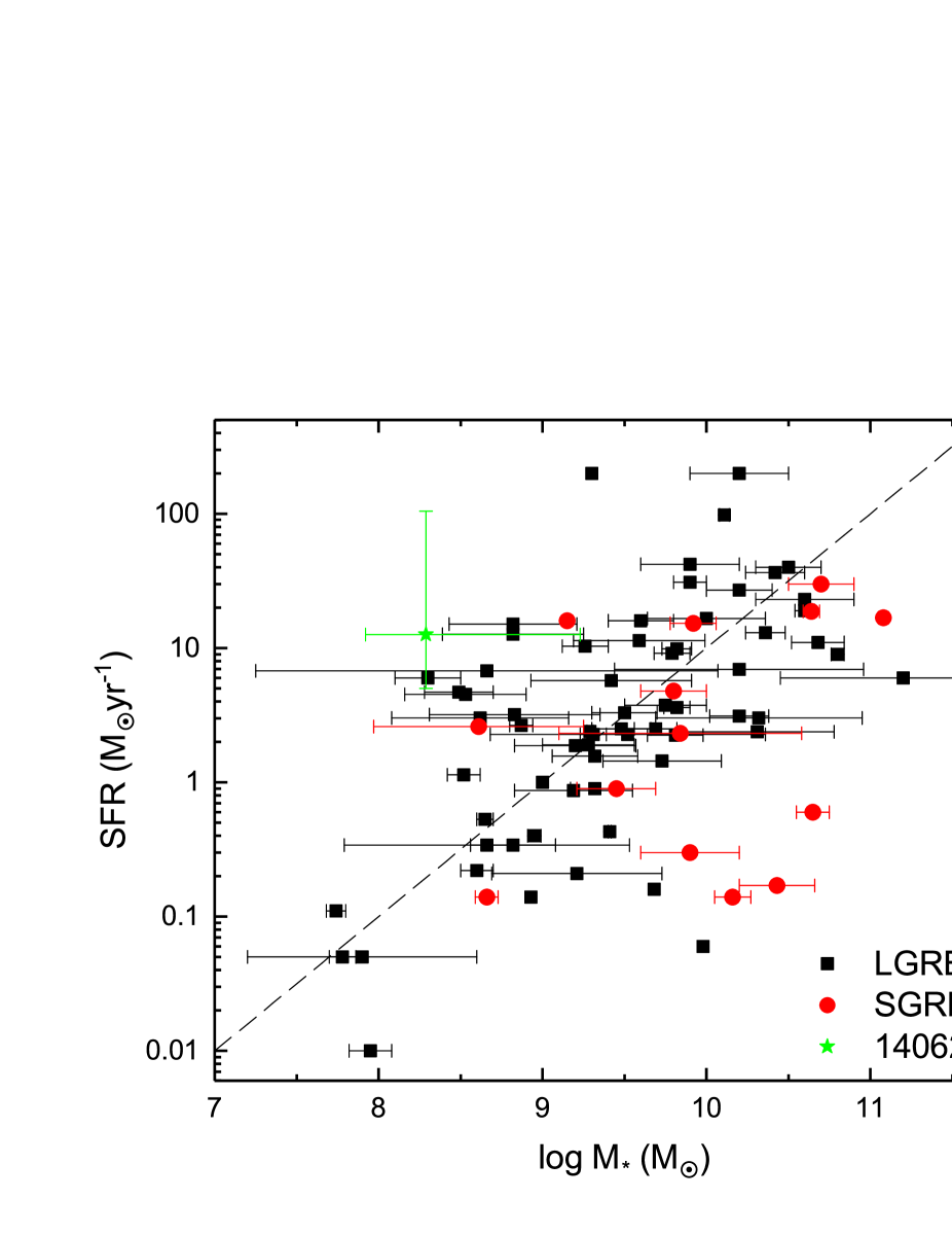
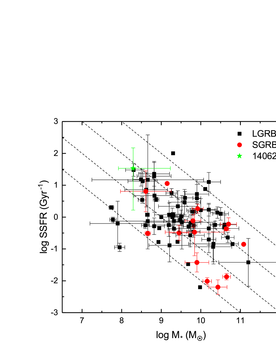
The best fit of the host galaxy SED suggests the host galaxy has a SFR of log(SFR)=$1.1_{-0.4}^{+0.9}$ M_⊙ yr^-1. Compared to other GRB host galaxies, the SFR is higher than the median value 2.5M_⊙ yr^-1 (Savaglio et al. 2009), but within 2$\sigma$ of the distribution. The host galaxy is consistent with the SFR and stellar mass correlation for star-forming galaxies, known as the star formation main sequence (Daddi et al. 2007), while it is at the edge of the distribution in the GRB sample shown in Figure 10 (Savaglio et al. 2009). This may indicate the mass of this galaxy is lower than other semi-SFR galaxies, although the errors are fairly large. The specific SFR is higher than the average value of  0.8Gyr^-1, but it follows the correlation between the SSFRs and the stellar mass (Christensen et al. 2004; Savaglio et al. 2009), as shown in Figure 11. The growth timescale in this case is lower than the Hubble time (Savaglio et al. 2009) at the burst distance, which suggests the galaxy is in a bursty mode.

Damped Lyman-alpha  (DLA; Wolfe et al. 1986, 2005) systems trace the bulk of neutral hydrogen available for star formation processes and are usually found in the lines of sight towards quasars  (QSOs; Noterdaeme et al. 2012; Sánchez-Ramírez et al. 2016) and GRBs (Fynbo et al. 2009; Thöne et al. 2013). Since GRBs are produced in star-forming regions, their sight-lines probe their surrounding neutral environments within a few hundred parsecs of the sites of the bursts (Vreeswijk et al. 2013; D’Elia et al. 2014). Hence, burst afterglow absorption spectroscopy at z $\geq$1.8 (for which the Lyman-alpha absorption line is red-shifted out of the atmospheric blue cut-off) provides a unique tool to investigate the amount of metals produced by vicinal star formation process. At a redshift of 2.276, GRB 140629A is therefore at a suitable distance from which we were able to obtain the constituents of the GRB environment.

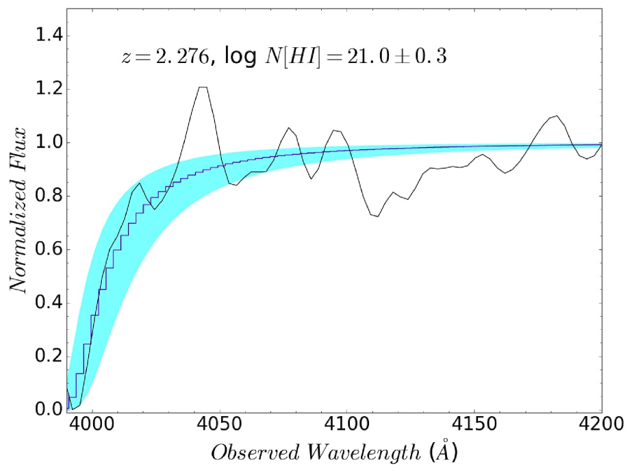
In order to investigate the neutral hydrogen content at the redshift of the host galaxy, we fitted the red damping wing of the Lyman-alpha absorption with the Voigt profile using the same prescription and tools described in Sánchez-Ramírez et al. (2016), obtaining a column density value of log $N_{HI}$=21.0$\pm$0.3, as shown in Figure 12. The large error in the fit mostly comes from the uncertainties in the continuum determination due to the low S/N at the blue end of the spectra. In particular, the neutral hydrogen column density is the characteristic indicator with which to distinguish if the host galaxy is a DLA system, by definition of $N_{HI}\geq 2\times 10^{20}$cm^-2(Wolfe et al. 2005). Therefore, the associated absorption system is technically classified as a DLA.

The measured column density is lower than the peak value $N_{HI}=10^{21.5}$cm^-2 found in the GRB-DLAs distribution  (Fynbo et al. 2009), but is still higher than the mean value of QSO-DLAs. Compared to other GRB-DLAs, this one does not show any properties distinct to the sample of bursts in Figure 4 of  Toy et al. (2016). This value is unusual in the QSO-DLA sample, but frequently observed in GRB sight-lines, suggesting once more that both samples are drawn from distinct populations.

In addition, we also identified strong high-ionisation lines, such as C IV, Si IV, and N V, which are present at the redshift of the absorber. In a previous analysis, it was found that the EWs of the GRB absorption feature are, on average, 2.5 times larger than those in QSO-DLAs (de Ugarte Postigo et al. 2012). As shown in Table 3, those features in GRB 140629A are still consistent and even have an excess on the high-ionisation lines, which is at least six times larger than the median value from QSO sample. Therefore, this burst also provides evidence for EWs in GRB-DLA systems being larger than those in QSO-DLAs. That may imply that GRBs are produced inside the most luminous regions of star-forming galaxies and that the light from the burst has to interact with much more host galaxy material. The N V lines can be used to trace collisionally ionised gas near long GRBs, since $N^{3+}$ has a high ionisation potential that makes the production of $N^{4+}$ difficult. The cold N V lines indicate that the GRB progenitor occurred within a dense environment $n\geq 10^{3}$cm^-2 (Prochaska et al. 2008) within the photo-ionisation scenario. This indirectly supports the dense medium found through numerical modelling of GRB 140629A. Nevertheless, we can neither constrain the distance of the N V absorption to the progenitor, nor the metal abundance owing to the low signal-to-noise ratio and resolution of the spectrum.

Figure 10: Plot of SFR vs. stellar mass for a sample of GRB hosts, inferred from template fitting to their photometric SEDs. The host of GRB 140629A is shown by a green star. Black squares and red dots represent the long burst and short burst hosts with SFRs measured from GHostS from 1997 to 2014 (Savaglio et al. 2006, 2009). The dashed line indicates a constant specific SFR of 1 Gyr^-1.

Figure 11: Plot of specific SFR vs. stellar mass for a sample of GRB hosts, inferred from template fitting to their photometric SEDs. The host of GRB 140629A is shown by a green star. Black dots indicate burst hosts with SFRs measured from GHostS from 1997 to 2014 (Savaglio et al. 2006, 2009). The dashed lines indicate the constant specific SFR of 0.1, 1, 10, and 100 Gyr^-1 from left to right.

Figure 12: Voigt profile fit to the DLA in the spectrum of GRB 140629A. The figure shows the data (black solid line) and the best fit damped profile (blue solid line) with its 1$\sigma$ confidence interval (cyan area).

5 Conclusions

Thanks to the rapid response of several robotic telescopes and continued follow up by larger facilities, in this paper we are able, to present multiwavelength photometric and spectroscopic observations of the long duration GRB 140629A, providing a unique dataset on which to test models for this GRB. A detailed analysis of this burst was carried out to uncover the jet and host galaxy properties. This analysis is based on the data obtained by MASTER net, OSN, BOOTES, GTC, and BTA, as well as the public data from Swift and Spitzer. Optical spectroscopy obtained with BTA shows absorption features at a redshift of z=$2.276\pm 0.001$ for this burst.

The signals in two orthogonal polarisations, measured by the MASTER telescope of GRB 140629A, set an upper limit of 18% at 1$\sigma$ confidence level which implies that it is a weakly polarised burst and that synchrotron radiation dominates the afterglow emission. Using the closure relations, we found that the afterglow in X-ray and optical bands can be well explained by a long-lasting central engine which produces continued energy injection at the beginning. After the end of energy injection, the normal decay phase is observed in both bands. The scenario in which a blast wave jet expands in a constant density ISM with slow cooling electrons, in the range $\upsilon_{m}<\upsilon_{o}<\upsilon_{x}<\upsilon_{c}$, can describe this burst well during the phases with and without energy injection. We identify the final X-ray break at 31000 s as a jet break. This break is achromatic and is observed in the optical at the same time and has break times consistent at 1$\sigma$. The afterglow is well explained by a single component outflow.

We also attempted to model the broadband data with a blast wave jet model based on the prescription of Zhang et al. (2015). The modelled result shows that this burst has a total energy release of $1.4\times 10^{54}$ergs with an opening angle of $6.7^{\circ}$ viewed $3.8^{\circ}$ off-axis. In addition, a high circumstellar density is obtained from modelling and is also inferred indirectly from the identification of a high ionisation line (N V).

After correcting for redshift and the opening angle, for GRB 140629A we find the peak energy in the rest frame and collimation-corrected energy are consistent with the Ghirlanda and Amati relations but not with the Liang-Zhang relation. The optical light curve displays a peak, which we identified as the afterglow onset produced by the forward shock which is the $\varGamma_{0}$ indicator. The onset is found at 181 s and indicates an initial Lorentz factor of 82-118.

Based on analysis of the host galaxy photometry, a low mass galaxy template with a SFR of log(SFR)=$1.1_{-0.4}^{+0.9}$ M_⊙ yr^-1 at an age of $1.14_{-0.35}^{+1.03}$Gyr is obtained. This result implies the host galaxy is consistent with the star formation main sequence in a star-forming galaxy. Fitting the spectroscopy at  4000$\AA$ with a Voigt profile, a neutral hydrogen density log$N_{HI}=21.0\pm 0.3$ derived indicates that we detect a DLA system in the GRB host galaxy.

——————————-

Table 8: Photometric observations at the GRB 140629A field at optical wavelengths. No correction for galactic extinction is applied.

Ins.	Band	T-T0 (s)	Exp(s)	Mag	Err
UVOT	$v$	643	10	15.30	0.09
UVOT	$v$	817	10	15.57	0.10
UVOT	$v$	4219	100	17.72	0.14
UVOT	$v$	5654	100	18.10	0.14
UVOT	$v$	10933	453	18.99	0.10
UVOT	$v$	23772	93	19.75	0.40
UVOT	$v$	40923	205	20.74	0.65
UVOT	$v$	74215	454	¿22.2	nan
UVOT	$v$	91482	6229	22.19	1.54
UVOT	$v$	142800	11769	¿22.1	nan
UVOT	$v$	265545	25697	¿23.9	nan
UVOT	$v$	328350	54	¿21.9	nan
UVOT	$b$	569	10	15.70	0.06
UVOT	$b$	742	10	15.94	0.07
UVOT	$b$	5039	100	18.45	0.08
UVOT	$b$	6474	100	18.76	0.10
UVOT	$b$	27297	281	20.45	0.20
UVOT	$b$	44612	233	22.08	1.43
UVOT	$b$	56976	3651	22.00	0.38
UVOT	$b$	80901	364	22.26	0.85
UVOT	$b$	142563	11702	22.59	1.21
UVOT	$b$	264961	25578	23.41	2.01
UVOT	$b$	328171	42	¿21.5	nan
UVOT	$u$	313	5	14.52	0.08
UVOT	$u$	323	5	14.57	0.08
UVOT	$u$	333	5	14.69	0.08
UVOT	$u$	343	5	14.56	0.08
UVOT	$u$	353	5	14.65	0.08
UVOT	$u$	363	5	14.77	0.08
UVOT	$u$	373	5	14.89	0.09
UVOT	$u$	383	5	14.72	0.08
UVOT	$u$	393	5	14.81	0.08
UVOT	$u$	403	5	14.77	0.08
UVOT	$u$	413	5	14.86	0.09
UVOT	$u$	423	5	14.92	0.09
UVOT	$u$	433	5	14.89	0.09
UVOT	$u$	443	5	14.96	0.09
UVOT	$u$	453	5	14.90	0.09
UVOT	$u$	463	5	15.05	0.09
UVOT	$u$	473	5	15.01	0.09
UVOT	$u$	483	5	15.13	0.10
UVOT	$u$	493	5	14.94	0.09
UVOT	$u$	503	5	15.07	0.09
UVOT	$u$	513	5	15.14	0.10
UVOT	$u$	523	5	15.12	0.10
UVOT	$u$	533	5	15.20	0.10
UVOT	$u$	543	5	15.25	0.10
UVOT	$u$	553	5	15.23	0.10
UVOT	$u$	717	10	15.44	0.08
UVOT	$u$	4834	100	17.74	0.08
UVOT	$u$	6269	100	18.27	0.10
UVOT	$u$	16707	116	19.13	0.15
UVOT	$u$	34925	6	¿20.3	nan
UVOT	$u$	56063	3776	21.56	0.34
UVOT	$u$	69374	5761	21.79	0.41
UVOT	$u$	86665	6117	22.73	1.72
UVOT	$u$	108800	305	¿23.1	nan
UVOT	$u$	142443	11665	¿22.7	nan
UVOT	$u$	264669	25515	¿23.1	nan
UVOT	$u$	328082	42	¿21.6	nan
UVOT	$white$	101	5	15.21	0.05
UVOT	$white$	111	5	15.01	0.05
UVOT	$white$	121	5	14.89	0.05
UVOT	$white$	131	5	14.80	0.05
UVOT	$white$	141	5	14.76	0.05
UVOT	$white$	151	5	14.72	0.05
UVOT	$white$	161	5	14.56	0.05
UVOT	$white$	171	5	14.66	0.05
UVOT	$white$	181	5	14.61	0.05
UVOT	$white$	191	5	14.70	0.05
UVOT	$white$	201	5	14.77	0.05
UVOT	$white$	211	5	14.72	0.05
UVOT	$white$	221	5	14.72	0.05
UVOT	$white$	231	5	14.80	0.05
UVOT	$white$	241	5	14.70	0.05
UVOT	$white$	593	10	15.74	0.04
UVOT	$white$	767	10	16.05	0.05
UVOT	$white$	868	75	16.25	0.03
UVOT	$white$	5244	100	18.54	0.05
UVOT	$white$	6678	57	18.80	0.08
UVOT	$white$	57887	225	21.69	0.29
UVOT	$white$	142681	11739	¿24.4	nan
UVOT	$white$	265252	25641	¿27.0	nan
UVOT	$white$	328259	42	¿21.5	nan
UVOT	$uvw1$	692	10	17.52	0.33
UVOT	$uvw1$	4629	100	20.01	0.41
UVOT	$uvw1$	6064	100	20.71	0.68
UVOT	$uvw1$	15801	450	21.39	0.60
UVOT	$uvw1$	34019	450	22.02	0.96
UVOT	$uvw1$	51655	5523	¿21.8	nan
UVOT	$uvw1$	68467	5757	¿23.6	nan
UVOT	$uvw1$	85759	5610	¿21.7	nan
UVOT	$uvw1$	107894	450	21.83	1.27
UVOT	$uvm2$	677	10	20.05	0.86
UVOT	$uvw2$	628	10	18.96	0.89
OSN	V	24852	600	19.83	0.11
OSN	V	27020	600	19.96	0.11
OSN	V	29186	600	20.07	0.11
OSN	V	115713	600	22.63	0.19
OSN	V	117851	600	22.97	0.22
OSN	V	120677	600	23.11	0.30
OSN	I	25781	600	18.99	0.20
OSN	I	27944	600	19.14	0.20
OSN	I	29931	600	19.33	0.20
OSN	I	116628	600	22.17	0.35
OSN	I	119433	600	22.29	0.33
OSN	I	121592	600	22.03	0.46
OSN	R	24537	300	18.89	0.15
OSN	R	25469	300	18.89	0.15
OSN	R	26393	300	19.03	0.15
OSN	R	26706	300	19.04	0.15
OSN	R	27632	300	19.06	0.15
OSN	R	28557	300	19.09	0.15
OSN	R	28871	300	19.17	0.15
OSN	R	29798	300	19.22	0.15
OSN	R	30723	300	19.28	0.15
OSN	R	115404	300	21.89	0.27
OSN	R	116320	300	21.97	0.26
OSN	R	117235	300	22.32	0.34
OSN	R	117543	2798	21.94	0.20
OSN	R	120369	2130	21.90	0.22
OSN	R	376511	5329	22.65	0.27
BOOTES	i	28937	1200	19.57	0.18
BOOTES	i	30413	1800	19.74	0.18
BOOTES	i	32305	1800	19.94	0.21
BOOTES	i	34310	1800	20.17	0.24
BOOTES	i	40041	2100	20.51	0.30
BOOTES	i	42288	2700	¿19.97	nan
BOOTES	i	45521	2640	¿19.65	nan
GTC	Sloan-g	$2.1\times 10^{7}$	140$\times$3	¿24.7	nan
GTC	Sloan-r	$2.1\times 10^{7}$	90	¿24.3	nan
GTC	Sloan-i	$2.1\times 10^{7}$	90$\times$4	¿24.6	nan
GTC	Sloan-g	$8.2\times 10^{7}$	$150\times 7$	25.01	0.20
GTC	Sloan-r	$8.2\times 10^{7}$	$120\times 7$	24.94	0.24
GTC	Sloan-i	$8.2\times 10^{7}$	$90\times 8$	24.71	0.32
Spitzer	3.6$\mu$m	$2.9\times 10^{7}$	$100\times 72$	22.01	1.00
MASTER-net
Amur	P$\backslash$	37	10	14.26	0.06
Amur	P$\backslash$	72	10	14.48	0.06
Amur	P$\backslash$	111	20	14.06	0.08
Amur	P$\backslash$	151	30	13.78	0.13
Amur	P$\backslash$	206	40	13.86	0.11
Amur	P$\backslash$	277	50	14.15	0.07
Amur	P$\backslash$	348	60	14.61	0.06
Amur	P$\backslash$	443	80	14.70	0.07
Amur	P$\backslash$	550	100	15.05	0.13
Amur	P$\backslash$	672	120	15.23	0.17
Tunka	P$\backslash$	1156	180	16.50	0.35
Tunka	C	2725	180	16.85	0.09
Tunka	V	2924	180	17.06	0.08
Tunka	R	2968	180	16.62	0.08
Tunka	V	3172	180	17.59	0.13
Tunka	R	3218	180	16.88	0.09
Tunka	V	3426	180	17.49	0.12
Tunka	R	3471	180	16.87	0.09
Tunka	V	3691	180	17.49	0.12
Tunka	R	3737	180	17.11	0.11
Tunka	V	3941	180	17.56	0.13
Tunka	R	3987	180	16.98	0.10
Tunka	V	4188	180	17.76	0.16
Tunka	R	4233	180	17.23	0.12
Tunka	P-	4553	180	17.87	0.23
Tunka	P$|$	4553	180	17.55	0.14
Tunka	P$|$	4803	180	17.72	0.15
Tunka	P-	4803	180	17.79	0.22
Tunka	P-	5046	180	17.81	0.22
Tunka	P$|$	5047	180	17.84	0.17
Tunka	P-	5287	180	17.92	0.24
Tunka	P$|$	5289	180	17.98	0.19
Tunka	P$|$	5531	180	17.90	0.17
Tunka	P-	5533	180	17.87	0.23
Tunka	P-	5778	180	18.38	0.32
Tunka	P$|$	5778	180	18.29	0.23
Tunka	P$|$	6023	180	18.16	0.21
Tunka	P-	6025	180	18.08	0.27
Tunka	P$|$	6289	180	18.19	0.21
Tunka	P-	6293	180	18.13	0.28
Tunka	P-	6534	180	18.25	0.30
Tunka	P$|$	6534	180	18.18	0.21
Tunka	P-	6775	180	18.34	0.31
Tunka	P$|$	6777	180	18.41	0.25
Tunka	P$|$	7016	180	18.15	0.21
Tunka	P-	7019	180	18.12	0.27
Tunka	P-	7257	180	18.07	0.27
Tunka	P$|$	7258	180	18.13	0.21
Tunka	P-	7505	180	18.25	0.30
Tunka	P$|$	7507	180	18.25	0.22
Tunka	P$|$	7748	180	18.26	0.22
Tunka	P-	7748	180	18.45	0.34
Tunka	P-	7990	180	18.99	0.45
Tunka	P$|$	7991	180	18.33	0.24
Tunka	P-	8233	180	18.34	0.31
Tunka	P$|$	8234	180	18.34	0.24
Tunka	P$|$	8490	180	18.37	0.24
Tunka	P-	8491	180	18.59	0.36
Tunka	P-	8733	180	18.16	0.28
Tunka	P$|$	8734	180	18.23	0.22
Tunka	P-	8976	180	18.30	0.31
Tunka	P$|$	8977	180	18.35	0.24
Tunka	P-	9228	180	18.43	0.33
Tunka	P$|$	9229	180	18.40	0.25
Tunka	P$|$	9471	180	18.50	0.26
Tunka	P-	9471	180	18.93	0.43
Tunka	P-	9711	180	18.09	0.27
Tunka	P$|$	9716	180	18.59	0.28
Tunka	P$|$	9952	180	18.58	0.28
Tunka	P-	9953	180	19.08	0.47
Tunka	P-	10189	180	18.70	0.38
Tunka	P$|$	10191	180	18.78	0.31
Tunka	P-	10431	180	19.07	0.47
Tunka	P$|$	10432	180	18.68	0.30
Tunka	P-	10682	180	18.42	0.33
Tunka	P$|$	10684	180	18.75	0.31
Tunka	P-	10923	180	19.21	0.50
Tunka	P$|$	10924	180	18.86	0.33
Tunka	P$|$	11175	180	18.79	0.32
Tunka	P-	11176	180	20.13	0.75
Tunka	P-	11431	180	18.87	0.42
Tunka	P$|$	11431	180	18.50	0.26
Tunka	P-	11686	180	19.18	0.49
Tunka	P$|$	11688	180	19.09	0.38
Tunka	P-	11933	180	18.62	0.37
Tunka	P$|$	11934	180	18.45	0.26
Tunka	P-	12173	180	19.88	0.67
Tunka	P$|$	12175	180	18.57	0.28
Tunka	P-	12412	180	18.61	0.37
Tunka	P$|$	12413	180	18.67	0.29
Tunka	P-	12652	180	18.51	0.35
Tunka	P$|$	12654	180	18.82	0.32
Tunka	P$|$	12905	180	17.61	0.14
Tunka	P$|$	13152	180	18.32	0.23
Tunka	P-	13394	180	18.29	0.31
Tunka	P$|$	13396	180	18.70	0.30
Tunka	P$|$	13638	180	18.87	0.33
Tunka	P$|$	13882	180	19.07	0.37
Tunka	P$|$	14119	180	18.78	0.32
Tunka	P$|$	14347	180	18.73	0.31
Tunka	P$|$	14586	180	18.50	0.26
Tunka	P$|$	14819	180	18.91	0.34
Tunka	P$|$	15059	180	20.17	0.68
Tunka	P$|$	15301	180	19.06	0.37
Tunka	P$|$	15550	180	19.81	0.56
Tunka	P$|$	15799	180	18.97	0.35
Tunka	P$|$	16057	180	19.91	0.59
Tunka	P$|$	16302	180	18.54	0.27
Tunka	P$|$	16553	180	20.11	0.66
Kislovodsk	C	22078	1080	19.74	0.13
Kislovodsk	R	22078	1080	19.42	0.22
Kislovodsk	C	23985	1980	19.42	0.13
Kislovodsk	R	24382	1800	19.19	0.22
Kislovodsk	C	26759	1620	19.78	0.13
Kislovodsk	R	26759	2160	19.88	0.22

Figure 13: Triangle plot of the MCMC fitting to our simulation-based model. It shows the posterior distribution and the correlation between the parameters.