New Early Dark Energy
Abstract
New measurements of the expansion rate of the Universe have plunged the standard model of cosmology into a severe crisis. In this letter, we propose a simple resolution to the problem that relies on a first order phase transition in a dark sector in the early Universe, before recombination. This will lead to a short phase of a New Early Dark Energy (NEDE) component and can explain the observations. We model the false vacuum decay of the NEDE scalar field as a sudden transition from a cosmological constant source to a decaying fluid with constant equation of state. The corresponding fluid perturbations are covariantly matched to the adiabatic fluctuations of a sub-dominant scalar field that triggers the phase transition. Fitting our model to measurements of the cosmic microwave background (CMB), baryonic acoustic oscillations (BAO, and supernovae (SNe) yields a significant improvement of the best-fit compared with the standard cosmological model without NEDE. We find the mean value of the present Hubble parameter in the NEDE model to be ( C.L.).
pacs:
98.80.Cq,98.80.-kI Introduction
Recent measurements of the expansion of the Universe have led to an apparent crisis for the standard model of cosmology, the CDM model. Within the CDM model, we can calculate the evolution of the Universe from the earliest times until today, and until recently all our measurements were consistent with the model. In particular, we can use the measurements of the CMB radiation to infer the present value of the Hubble parameter . If the CDM model is correct, this value will have to agree with the value obtained by directly measuring the expansion rate today using supernovae redshift measurements. Now, the problem is that the measurements, direct and indirect, do not agree, and this puts the CDM model in a crisis.
The most precise measurements we have of the temperature fluctuations, polarization and lensing in the CMB radiation are from the Planck satellite, which, assuming the CDM model, infers the value of the expansion rate today to be Aghanim:2018eyx . Comparing that with the expansion rate measured from Cepheids-calibrated supernovae by the SH0ES team Riess:2019cxk , , there is a discrepancy. Other measurements of the current Hubble rate, such as H0LiCoW Chen:2019ejq , are also significantly discrepant with the Planck measurement Verde:2019ivm .
The Planck measurement of the CMB is a very clean experiment with the systematics well under control, and it is therefore unlikely that there is non-understood systematics in the CMB measurements that can explain the discrepancy. The local supernova observations, on the other hand, involves astronomical distance measurements, which are notoriously difficult, and have been plagued by non-understood systematic errors in the past. Various possible sources of systematics have been considered extensively in the literature already Davis:2019wet ; Wojtak:2013gda ; Odderskov:2017ivg ; Wu:2017fpr . So far, astronomers have no commonly accepted idea of possible systematic effects to explain the discrepancy, and an often echoed conclusion is that new physics beyond the CDM model is required to resolve the tension (see e.g., Bernal:2016gxb ; Knox:2019rjx ). While it is important to continue to look for possible systematic effects, in the present paper, we will rather consider a simple solution in terms of new physics.
We will study the possibility that a first order phase transition in a dark sector at zero temperature happened shortly before recombination in the early Universe. Such a phase transition will have the effect of lowering an initially high value of the cosmological constant in the early Universe down to the value today, inferred from the measurement of . Effectively this means that there has been an extra component of dark energy in the early Universe, providing a short burst of additional repulsion. Currently, an extra component of Early Dark Energy (EDE) seems to be a promising way to resolve the tension between the early and late measurements of Poulin:2018dzj ; Poulin:2018cxd ; Smith:2019ihp ; Lin:2019qug ; Kaloper:2019lpl ; Alexander:2019rsc ; Hardy:2019apu ; Knox:2019rjx . So far, people have typically considered a dynamical EDE component that disappears due to a second order phase transition of a slowly rolling scalar field.111The general idea of having an early dark energy component is older and dates back to Wetterich:2004pv ; Doran:2006kp . Such scenarios have complications if monomial potentials are used both at background and perturbative level Agrawal:2019lmo ; Smith:2019ihp , as one needs the potential to be steep and anharmonic at the bottom to end up with a sufficiently stiff fluid but also flat initially to achieve a sound speed for a large enough range of sub-horizon modes. While this problem can be overcome by using specific terms from the non-perturbative form of the axion potential Poulin:2018dzj ; Poulin:2018cxd ; Smith:2019ihp , it represents a non-generic choice Kaloper:2019lpl .222For other proposals to address the Hubble tension operational at late and/or early times see DiValentino:2016hlg ; Kumar:2016zpg ; Kumar:2017dnp ; DiValentino:2017iww ; DiValentino:2017zyq ; Addison:2017fdm ; Buen-Abad:2017gxg ; Mortsell:2018mfj ; Vagnozzi:2018jhn ; Poulin:2018zxs ; Yang:2018euj ; DEramo:2018vss ; Guo:2018ans ; Aylor:2018drw ; Kreisch:2019yzn ; Raveri:2019mxg ; Keeley:2019esp ; DiValentino:2019exe ; Gelmini:2019deq ; Pan:2019gop ; Vagnozzi:2019ezj ; Visinelli:2019qqu ; Pan:2019hac ; DiValentino:2019ffd ; Arendse:2019hev .
On the other hand, we believe that a first order phase transition holds in it the potential to fully resolve the discrepancy between the early and late measurements of much more naturally. In addition, a first order phase transition will lead to different experimental signatures in the details of the CMB and large-scale structure as well as gravitational waves.
Below we explore the simplest NEDE model. For more details and generalizations of the model, as well as a detailed comparison with other models, we refer the reader to our longer subsequent paper long-one .
II The Model
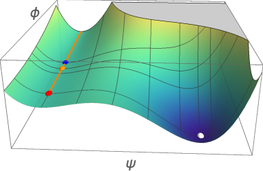
In order to have a change in the vacuum energy due to a field that undergoes a first order phase transition, we will consider a scalar field with two non-degenerate minima at zero temperature. However, if the tunneling probability from the false to the true vacuum is initially high, the field will tunnel immediately and NEDE never makes a sizable contribution. On the other hand, once tunneling commences, we need a large rate in order to produce enough bubbles of true vacuum that will quickly collide. If the rate is too small, then part of the Universe will be in the true and part of it in the false vacuum, which will lead to large inhomogeneities ruled out by observations. We therefore require an additional sub-dominant trigger field that, at the right moment, makes the tunneling rate very high. Analogous to previously considered mechanisms for ending inflation in Linde:1990gz ; Adams:1990ds ; Copeland:1994vg ; Cortes:2009ej , we will therefore consider models with a general potential of the form,
where is the tunneling field and is the trigger field. The sub-dominant trigger field will be frozen as long as its mass is smaller than the Hubble rate, but as soon as the Hubble rate drops below its mass, it will start decaying and this will trigger the tunneling of the field. For a second minimum to develop after the point of inflection, we need to impose , . In Fig. 1, we show a 3D visualization of the evolution of the potential as the trigger field, , starts evolving along the orange path opening up the new vacuum for , to which it tunnels with high probability.
The decay rate per unit volume is , where is a determinant factor which is generically set by the energy scale of the phase transition Callan:1977pt ; Linde:1981zj and is the Euclidian action corresponding to a so-called bounce solution Coleman:1977py . While it is possible to find an analytic expression in the thin wall limit for a single field, the general case requires a numerical approach. In long-one we argue that a good approximation of the Euclidian action (describing the potential as being effectively one-dimensional) can be written as
| (2) |
with numerically determined coefficients Adams:1993zs , , and
| (3) |
We see that becomes large as and vanishes as . As a result, the tunneling rate is suppressed when is frozen at a sufficiently large initial field value (corresponding to ) and becomes maximal as once the Hubble drag is released (corresponding to ).
At early times, we require the transition rate to be highly suppressed, which fixes the initial value of the trigger field, , and can be satisfied consistently with the condition that , which is sufficient to ensure that the contribution of to the total energy density is sub-dominant.
Now, we also have to ensure that NEDE, given by the potential energy in the field, gives a sizable contribution to the energy budget at the time where bubble percolation of the vacuum becomes efficient. We can quantify it in terms of the ratio , where is the liberated vacuum energy and the total energy density. If the transition occurs at a redshift of order , , and , we have and an ultra-light mass scale of order . A microphysical model explaining the mass hierarchy between the and the scale would be a model of axion monodromy with two axion fields (see Kaloper:2008fb for a field theory version). Here, the masses are protected by softly broken shift symmetries.
We also have to make sure that the nucleation itself happens sufficiently quickly. To that end, we define the percolation parameter , where we approximated . Provided , a large number of bubbles is nucleated within one Hubble patch and one Hubble time. In fact, for the above choice of parameters, the huge hierarchy between the scalar masses, , implies that only requires , which according to (2) and (3) can be easily satisfied as . This means that percolation is extremely efficient and will cover the entire space with bubbles of true vacuum in a tiny fraction of a Hubble time. Therefore, we can treat it as an instantaneous process on cosmological time scales, which takes place at time .
As the space is being filled with bubbles of true vacuum, they expand and start to collide when they are of physical size today . Thus, they do not induce anisotropies on scales large enough to be probed using CMB measurements. This phase is governed by complicated dynamics, which can be studied analytically only in simplified two-bubble scenarios as in Hawking:1982ga . As part of the collision process, the complicated condensate starts to decay. Microscopically, the released free energy gets converted into anisotropic stress on small scales, which we expect, after partially being converted to gravitational radiation, to decay as , similar to a stiff fluid component. We leave it for future work to substantiate this picture, which assumes a decoupling of small and large scales, through explicit numerical studies.
III Matching conditions
We use a simple background model describing the instantaneous transition from a background fluid with an equation of state (e.o.s.) parameter that changes from to ,
| (4) |
where the transition happens at time . In terms of our field theory model in (II), this corresponds to a situation where all of the liberated vacuum energy is transferred to a fluid with e.o.s. parameter , and where according to the considerations above, we expect . Describing the bubble wall condensate in terms of a fluid with a constant is a simplifying assumption, which should ultimately be tested with lattice field theory techniques resolving the scalar field and its perturbations explicitly.333The importance of tracking field perturbations was highlighted recently in the case of the second-order, single-field EDE model in Agrawal:2019lmo , although after the NEDE transition, the frequency of the fluctuations is much higher, and the course grained fluid description is expected to be a better approximation.
III.1 Background Matching
The above condition fixes the evolution of the background energy density uniquely,
| (5) |
where . The energy density of NEDE is normalized with respect to the true vacuum and continuous across the transition. The discontinuity of a time dependent function across the transition surface at time is denoted as
| (6) |
Applying this operation to the Friedmann equations, we then find
| (7a) | ||||
| (7b) | ||||
where we used the continuity of the background energy density, , which holds due to (5) and the instantaneous character of the transition. The derivation of (7b) also assumes that the e.o.s. of all other fluid components (except for NEDE) is preserved during the transition. Besides the NEDE component, we also track the evolution of the sub-dominant field to turn on the phase transition.
III.2 Perturbation Matching
Before the decay we can set the perturbations of the NEDE fluid to zero as it behaves as a (non-fluctuating) cosmological constant. This raises the issue of how to initialize perturbations at time . Moreover, since the transition is allowed to happen at a relatively late stage in the evolution of the primordial plasma (in the extreme case right before recombination), we cannot assume that all relevant modes are outside the horizon. In the specific case of our two-field model, we use the trigger field to define the transition surface , explicitly,
| (8) |
This is motivated by the dependence of the parameter in (3) which controls the exponential in the tunneling rate through (2). As a consequence, fluctuations in lead to spatial variations of the time at which the decay takes place. These variations, , then provide the initial conditions for the fluctuations in the NEDE fluid after the phase transition.
In order to match the conventions used in the Boltzmann code community, we work in synchronous gauge,
| (9) |
where in momentum space
| (10) |
and . In the following we will make use of the equations for the metric perturbations that are first order in time derivatives Ma:1995ey ,
| (11a) | ||||
| (11b) | ||||
where and are the total divergence of the fluid velocity and the total energy density perturbation, respectively. The dynamical equations have to be supplemented with Israel’s matching conditions Israel:1966rt ; Deruelle:1995kd . They relate the time derivatives of and before and after the transition,
| (12) |
where is specified in (7b), and we used the residual gauge freedom in the synchronous gauge to bring the matching conditions on this simple form. We further find that all perturbations without a derivative, including the fluid sector, are continuous, i.e. , where . This does not apply to NEDE perturbations because the derivation assumed that the e.o.s. of a particular matter component is not changing during the transition, in contrast with (4). As argued before, we can consistently set
| (13) |
We further introduce the notation and to denote the fluctuations right after the transition. We can now evaluate the discontinuity of Einstein’s equations (11) in order to fix and , providing the initial conditions for the NEDE perturbations after the transition. Using (12) and (7b), we have
| (14a) | ||||
| (14b) | ||||
These two equations together with the junction conditions (12) will allow us to consistently implement our model in a Boltzmann code. In order to close the differential system of the perturbed fluid equations, we set the rest-frame sound speed Hu:1998kj in the NEDE fluid to .
IV Data Analysis and Results
In order to fit the NEDE model to the CMB data, we have incorporated it into the Boltzmann code444The adapted CLASS code is publicly available on GitHub: https://github.com/flo1984/TriggerCLASS CLASS Lesgourgues:2011re ; Blas:2011rf . To that end, we made the simplifying assumption that all liberated vacuum energy is ultimately converted to small scale anisotropic stress and gravitational radiation described as a fluid with . As a specific choice for our data fit, we take the midpoint , which we relax in our subsequent paper long-one . In accordance with our microscopic model the decay is triggered shortly before , where for definiteness we take (which avoids a tuning and is still compatible with a quick decay). The sub-dominant trigger field and its perturbations are evolved explicitly and matched to the fluid perturbations through (14). This scenario also assumes that there are no sizeable oscillations in around the true vacuum, which could give rise to an additional sub-dominant dust component. A more detailed discussion of the corresponding microscopic constraints is provided in Sec. IID in long-one .
The cosmological parameters are then extracted with the Monte Carlo Markov chain code MontePython Audren:2012wb ; Brinckmann:2018cvx , employing a Metropolis-Hastings algorithm. We perform a model comparison by computing the difference in Bayesian evidence (CDM) using the MultiNest algorithm (evidence tolerance 0.1 and 1000 live-points) Feroz:2008xx ; Feroz:2013hea ; Buchner:2014nha . Compared to CDM, we introduce two new parameters: the fraction of NEDE before the decay, , and the logarithm of the mass of the trigger field , which defines the redshift at decay time, , via . In total, we vary eight parameters , on which we impose flat priors. The neutrino sector is modeled in terms of two massless and one massive species with . We impose the initial value to make sure that the trigger field is always sub-dominant and the tunneling rate at early times sufficiently suppressed.
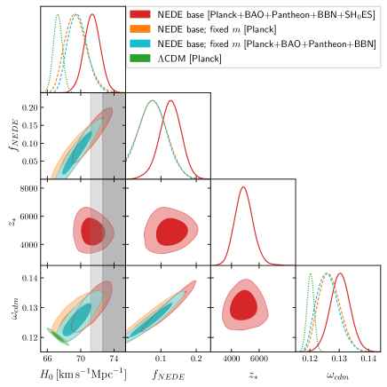
We will use the following data sets: the most recent SH0ES measurement, which is Riess:2019cxk ; the Pantheon data set Scolnic:2017caz comprised of 1048 SNe Ia in a range ; the large- BOSS DR 12 anisotropic BAO and growth function measurements at redshift , and based on the CMASS and LOWZ galaxy samples Alam:2016hwk , as well as small-z, isotropic BAO measurements of the 6dF Galaxy Survey Beutler:2011hx and the SDSS DR7main Galaxy sample Ross:2014qpa at and , respectively (collectively referred to as BAO); the Planck 2018 TT, TE, EE and lensing likelihood Aghanim:2019ame with all nuisance parameters; constraints on the primordial helium abundance from Aver:2015iza (referred to as BBN). We perform one likelihood analysis with all data sets combined (see red contours in Fig. 2), one where we only exclude the SH0ES value (turquoise contours) and one with Planck (TT, TE, EE and lensing) alone (orange contours). For the latter two, we fix in order to avoid sampling volume artifacts in the limit. While we provide an exhaustive discussion of this issue and also results without fixing in our subsequent paper long-one , here, we highlight the main findings supp_material .
For the analysis with all data sets, the best-fit improves by compared to CDM. This improvement is shared between SH0ES [(SH0ES) = -13.8] and the other data sets [(w/o SH0ES) = -1.8]. This observation is crucial at it shows that NEDE does not lead to new tensions. Instead, it also improves the overall fit to the other data sets.555There is a slight degradation of the large- BAO data set of (large- BAO + LSS) = 0.9, which we will explore in our future work about large-scale structure within NEDE Niedermann:2020qbw . Moreover, we find . The decay takes place at , and there is a non-vanishing NEDE fraction , excluding with a significance. This is also supported by the Bayesian evidence measure, which amounts to , corresponding to a “very strong” evidence on Jeffreys’ scale Efron .
This picture is further solidified by our runs without SH0ES, which lead to a (very similar) fit improvement of (Planck) and (Planck+BAO+Pantheon+BBN). In both cases, we find a evidence for a non-vanishing value of and a “weak” (but positive) Bayesian evidence of [when fixing ]. The mean values are and , respectively, which brings the Hubble tension down to , in turn justifying our joint analysis. In short, NEDE introduces an approximate degeneracy in the vs plane (see Fig. 2). The SH0ES measurement is then needed to select NEDE as the favored model.
V Conclusions
We have studied a NEDE model where the decay of NEDE happens through a first order phase transition. This makes our model unique compared to older EDE models (which all rely on a second order phase transition) both from a theoretical and phenomenological perspective. The NEDE model holds in it the potential to fully resolve the discrepancy in as inferred from early CMB and BAO measurements and late time distance ladder measurements. Our first most simplified implementation of the model (fixing as many free parameters as possible by making simple assumptions) already yields a significant improvement in the fit over the CDM model of when including the SH0ES measurement of . Crucially, this does not compromise the fit to the other data sets. Correspondingly, without including the SH0ES prior on , the Hubble tension is reduced to the level. We expect that the model will fit the data even better when the simplifying assumptions made in the present short paper are dropped in future work.
Acknowledgements.
We thank Edmund Copeland, José Espinosa, Nemanja Kaloper, Antonio Padilla and Kari Rummukainen for discussions and/or useful comments on the manuscript. This work is supported by Villum Fonden grant 13384. CP3-Origins is partially funded by the Danish National Research Foundation, grant number DNRF90.References
- (1) N. Aghanim et al. [Planck Collaboration], arXiv:1807.06209 [astro-ph.CO].
- (2) A. G. Riess, S. Casertano, W. Yuan, L. M. Macri and D. Scolnic, Astrophys. J. 876 (2019) no.1, 85 doi:10.3847/1538-4357/ab1422 [arXiv:1903.07603 [astro-ph.CO]].
- (3) G. C.-F. Chen et al., doi:10.1093/mnras/stz2547 arXiv:1907.02533 [astro-ph.CO].
- (4) L. Verde, T. Treu and A. G. Riess, Nature Astronomy 2019 doi:10.1038/s41550-019-0902-0 [arXiv:1907.10625 [astro-ph.CO]].
- (5) T. M. Davis, S. R. Hinton, C. Howlett and J. Calcino, Mon. Not. Roy. Astron. Soc. 490 (2019) no.2, 2948-2957 doi:10.1093/mnras/stz2652 [arXiv:1907.12639 [astro-ph.CO]].
- (6) R. Wojtak, A. Knebe, W. A. Watson, I. T. Iliev, S. Heß, D. Rapetti, G. Yepes and S. Gottlöber, Mon. Not. Roy. Astron. Soc. 438 (2014) no.2, 1805 doi:10.1093/mnras/stt2321 [arXiv:1312.0276 [astro-ph.CO]].
- (7) I. Odderskov, S. Hannestad and J. Brandbyge, JCAP 1703 (2017) 022 doi:10.1088/1475-7516/2017/03/022 [arXiv:1701.05391 [astro-ph.CO]].
- (8) H. Y. Wu and D. Huterer, Mon. Not. Roy. Astron. Soc. 471 (2017) no.4, 4946 doi:10.1093/mnras/stx1967 [arXiv:1706.09723 [astro-ph.CO]].
- (9) J. L. Bernal, L. Verde and A. G. Riess, JCAP 1610 (2016) 019 doi:10.1088/1475-7516/2016/10/019 [arXiv:1607.05617 [astro-ph.CO]].
- (10) L. Knox and M. Millea, Phys. Rev. D 101 (2020) no.4, 043533 doi:10.1103/PhysRevD.101.043533 [arXiv:1908.03663 [astro-ph.CO]].
- (11) V. Poulin, T. L. Smith, D. Grin, T. Karwal and M. Kamionkowski, Phys. Rev. D 98 (2018) no.8, 083525 doi:10.1103/PhysRevD.98.083525 [arXiv:1806.10608 [astro-ph.CO]].
- (12) V. Poulin, T. L. Smith, T. Karwal and M. Kamionkowski, Phys. Rev. Lett. 122 (2019) no.22, 221301 doi:10.1103/PhysRevLett.122.221301 [arXiv:1811.04083 [astro-ph.CO]].
- (13) T. L. Smith, V. Poulin and M. A. Amin, Phys. Rev. D 101 (2020) no.6, 063523 doi:10.1103/PhysRevD.101.063523 [arXiv:1908.06995 [astro-ph.CO]].
- (14) N. Kaloper, Int. J. Mod. Phys. D 28 (2019) no.14, 1944017 doi:10.1142/S0218271819440176 [arXiv:1903.11676 [hep-th]].
- (15) S. Alexander and E. McDonough, Phys. Lett. B 797 (2019) 134830 doi:10.1016/j.physletb.2019.134830 [arXiv:1904.08912 [astro-ph.CO]].
- (16) M. X. Lin, G. Benevento, W. Hu and M. Raveri, Phys. Rev. D 100 (2019) no.6, 063542 doi:10.1103/PhysRevD.100.063542 [arXiv:1905.12618 [astro-ph.CO]].
- (17) E. Hardy and S. Parameswaran, Phys. Rev. D 101 (2020) no.2, 023503 doi:10.1103/PhysRevD.101.023503 [arXiv:1907.10141 [hep-th]].
- (18) C. Wetterich, Phys. Lett. B 594 (2004), 17-22 doi:10.1016/j.physletb.2004.05.008 [arXiv:astro-ph/0403289 [astro-ph]].
- (19) M. Doran and G. Robbers, JCAP 06 (2006), 026 doi:10.1088/1475-7516/2006/06/026 [arXiv:astro-ph/0601544 [astro-ph]].
- (20) P. Agrawal, F. Y. Cyr-Racine, D. Pinner and L. Randall, [arXiv:1904.01016 [astro-ph.CO]].
- (21) E. Di Valentino, A. Melchiorri and J. Silk, Phys. Lett. B 761 (2016), 242-246 doi:10.1016/j.physletb.2016.08.043 [arXiv:1606.00634 [astro-ph.CO]].
- (22) S. Kumar and R. C. Nunes, Phys. Rev. D 94 (2016) no.12, 123511 doi:10.1103/PhysRevD.94.123511 [arXiv:1608.02454 [astro-ph.CO]].
- (23) S. Kumar and R. C. Nunes, Phys. Rev. D 96 (2017) no.10, 103511 doi:10.1103/PhysRevD.96.103511 [arXiv:1702.02143 [astro-ph.CO]].
- (24) E. Di Valentino, A. Melchiorri and O. Mena, Phys. Rev. D 96 (2017) no.4, 043503 doi:10.1103/PhysRevD.96.043503 [arXiv:1704.08342 [astro-ph.CO]].
- (25) E. Di Valentino, A. Melchiorri, E. V. Linder and J. Silk, Phys. Rev. D 96 (2017) no.2, 023523 doi:10.1103/PhysRevD.96.023523 [arXiv:1704.00762 [astro-ph.CO]].
- (26) G. E. Addison, D. J. Watts, C. L. Bennett, M. Halpern, G. Hinshaw and J. L. Weiland, Astrophys. J. 853 (2018) no.2, 119 doi:10.3847/1538-4357/aaa1ed [arXiv:1707.06547 [astro-ph.CO]].
- (27) M. A. Buen-Abad, M. Schmaltz, J. Lesgourgues and T. Brinckmann, JCAP 01 (2018), 008 doi:10.1088/1475-7516/2018/01/008 [arXiv:1708.09406 [astro-ph.CO]].
- (28) E. Mörtsell and S. Dhawan, JCAP 09 (2018), 025 doi:10.1088/1475-7516/2018/09/025 [arXiv:1801.07260 [astro-ph.CO]].
- (29) S. Vagnozzi, S. Dhawan, M. Gerbino, K. Freese, A. Goobar and O. Mena, Phys. Rev. D 98 (2018) no.8, 083501 doi:10.1103/PhysRevD.98.083501 [arXiv:1801.08553 [astro-ph.CO]].
- (30) V. Poulin, K. K. Boddy, S. Bird and M. Kamionkowski, Phys. Rev. D 97 (2018) no.12, 123504 doi:10.1103/PhysRevD.97.123504 [arXiv:1803.02474 [astro-ph.CO]].
- (31) W. Yang, S. Pan, E. Di Valentino, R. C. Nunes, S. Vagnozzi and D. F. Mota, JCAP 09 (2018), 019 doi:10.1088/1475-7516/2018/09/019 [arXiv:1805.08252 [astro-ph.CO]].
- (32) F. D’Eramo, R. Z. Ferreira, A. Notari and J. L. Bernal, JCAP 11 (2018), 014 doi:10.1088/1475-7516/2018/11/014 [arXiv:1808.07430 [hep-ph]].
- (33) R. Y. Guo, J. F. Zhang and X. Zhang, JCAP 02 (2019), 054 doi:10.1088/1475-7516/2019/02/054 [arXiv:1809.02340 [astro-ph.CO]].
- (34) K. Aylor, M. Joy, L. Knox, M. Millea, S. Raghunathan and W. L. K. Wu, Astrophys. J. 874 (2019) no.1, 4 doi:10.3847/1538-4357/ab0898 [arXiv:1811.00537 [astro-ph.CO]].
- (35) C. D. Kreisch, F. Y. Cyr-Racine and O. Doré, Phys. Rev. D 101 (2020) no.12, 123505 doi:10.1103/PhysRevD.101.123505 [arXiv:1902.00534 [astro-ph.CO]].
- (36) M. Raveri, Phys. Rev. D 101 (2020) no.8, 083524 doi:10.1103/PhysRevD.101.083524 [arXiv:1902.01366 [astro-ph.CO]].
- (37) R. E. Keeley, S. Joudaki, M. Kaplinghat and D. Kirkby, JCAP 12 (2019), 035 doi:10.1088/1475-7516/2019/12/035 [arXiv:1905.10198 [astro-ph.CO]].
- (38) E. Di Valentino, R. Z. Ferreira, L. Visinelli and U. Danielsson, Phys. Dark Univ. 26 (2019), 100385 doi:10.1016/j.dark.2019.100385 [arXiv:1906.11255 [astro-ph.CO]].
- (39) G. B. Gelmini, A. Kusenko and V. Takhistov, [arXiv:1906.10136 [astro-ph.CO]].
- (40) S. Pan, W. Yang, E. Di Valentino, E. N. Saridakis and S. Chakraborty, Phys. Rev. D 100 (2019) no.10, 103520 doi:10.1103/PhysRevD.100.103520 [arXiv:1907.07540 [astro-ph.CO]].
- (41) S. Vagnozzi, Phys. Rev. D 102 (2020) no.2, 023518 doi:10.1103/PhysRevD.102.023518 [arXiv:1907.07569 [astro-ph.CO]].
- (42) L. Visinelli, S. Vagnozzi and U. Danielsson, Symmetry 11 (2019) no.8, 1035 doi:10.3390/sym11081035 [arXiv:1907.07953 [astro-ph.CO]].
- (43) S. Pan, W. Yang, E. Di Valentino, A. Shafieloo and S. Chakraborty, JCAP 06 (2020) no.06, 062 doi:10.1088/1475-7516/2020/06/062 [arXiv:1907.12551 [astro-ph.CO]].
- (44) E. Di Valentino, A. Melchiorri, O. Mena and S. Vagnozzi, Phys. Dark Univ. 30 (2020), 100666 doi:10.1016/j.dark.2020.100666 [arXiv:1908.04281 [astro-ph.CO]].
- (45) N. Arendse, R. J. Wojtak, A. Agnello, G. C. F. Chen, C. D. Fassnacht, D. Sluse, S. Hilbert, M. Millon, V. Bonvin and K. C. Wong, et al. Astron. Astrophys. 639 (2020), A57 doi:10.1051/0004-6361/201936720 [arXiv:1909.07986 [astro-ph.CO]].
- (46) F. Niedermann and M. S. Sloth, Phys. Rev. D 102 (2020) no.6, 063527 doi:10.1103/PhysRevD.102.063527 [arXiv:2006.06686 [astro-ph.CO]].
- (47) A. D. Linde, Phys. Lett. B 249 (1990), 18-26 doi:10.1016/0370-2693(90)90521-7
- (48) F. C. Adams and K. Freese, Phys. Rev. D 43 (1991), 353-361 doi:10.1103/PhysRevD.43.353 [arXiv:hep-ph/0504135 [hep-ph]].
- (49) E. J. Copeland, A. R. Liddle, D. H. Lyth, E. D. Stewart and D. Wands, Phys. Rev. D 49 (1994) 6410 doi:10.1103/PhysRevD.49.6410 [astro-ph/9401011].
- (50) M. Cortes and A. R. Liddle, Phys. Rev. D 80 (2009) 083524 doi:10.1103/PhysRevD.80.083524 [arXiv:0905.0289 [astro-ph.CO]].
- (51) C. G. Callan, Jr. and S. R. Coleman, Phys. Rev. D 16 (1977) 1762. doi:10.1103/PhysRevD.16.1762
- (52) A. D. Linde, Nucl. Phys. B 216 (1983) 421 Erratum: [Nucl. Phys. B 223 (1983) 544]. doi:10.1016/0550-3213(83)90293-6, 10.1016/0550-3213(83)90072-X
- (53) S. R. Coleman, Phys. Rev. D 15 (1977) 2929 Erratum: [Phys. Rev. D 16 (1977) 1248]. doi:10.1103/PhysRevD.15.2929, 10.1103/PhysRevD.16.1248
- (54) F. C. Adams, Phys. Rev. D 48 (1993) 2800 doi:10.1103/PhysRevD.48.2800 [hep-ph/9302321].
- (55) N. Kaloper and L. Sorbo, Phys. Rev. Lett. 102 (2009) 121301 doi:10.1103/PhysRevLett.102.121301 [arXiv:0811.1989 [hep-th]].
- (56) S. W. Hawking, I. G. Moss and J. M. Stewart, Phys. Rev. D 26 (1982) 2681. doi:10.1103/PhysRevD.26.2681
- (57) C. P. Ma and E. Bertschinger, Astrophys. J. 455 (1995) 7 doi:10.1086/176550 [astro-ph/9506072].
- (58) N. Deruelle and V. F. Mukhanov, Phys. Rev. D 52 (1995) 5549 doi:10.1103/PhysRevD.52.5549
- (59) W. Israel, Nuovo Cim. B 44S10 (1966) 1 [Nuovo Cim. B 44 (1966) 1] Erratum: [Nuovo Cim. B 48 (1967) 463]. doi:10.1007/BF02710419, 10.1007/BF02712210
- (60) W. Hu, Astrophys. J. 506 (1998), 485-494 doi:10.1086/306274 [arXiv:astro-ph/9801234 [astro-ph]].
- (61) J. Lesgourgues, arXiv:1104.2932 [astro-ph.IM].
- (62) D. Blas, J. Lesgourgues and T. Tram, JCAP 1107 (2011) 034 doi:10.1088/1475-7516/2011/07/034 [arXiv:1104.2933 [astro-ph.CO]].
- (63) B. Audren, J. Lesgourgues, K. Benabed and S. Prunet, JCAP 1302 (2013) 001 doi:10.1088/1475-7516/2013/02/001 [arXiv:1210.7183 [astro-ph.CO]].
- (64) T. Brinckmann and J. Lesgourgues, arXiv:1804.07261 [astro-ph.CO].
- (65) F. Feroz, M. P. Hobson and M. Bridges, Mon. Not. Roy. Astron. Soc. 398 (2009), 1601-1614 doi:10.1111/j.1365-2966.2009.14548.x [arXiv:0809.3437 [astro-ph]].
- (66) F. Feroz, M. P. Hobson, E. Cameron and A. N. Pettitt, Open J. Astrophys. 2 (2019) no.1, 10 doi:10.21105/astro.1306.2144 [arXiv:1306.2144 [astro-ph.IM]].
- (67) J. Buchner, A. Georgakakis, K. Nandra, L. Hsu, C. Rangel, M. Brightman, A. Merloni, M. Salvato, J. Donley and D. Kocevski, Astron. Astrophys. 564 (2014), A125 doi:10.1051/0004-6361/201322971 [arXiv:1402.0004 [astro-ph.HE]].
- (68) D. M. Scolnic et al., Astrophys. J. 859 (2018) no.2, 101 doi:10.3847/1538-4357/aab9bb [arXiv:1710.00845 [astro-ph.CO]].
- (69) S. Alam et al. [BOSS Collaboration], Mon. Not. Roy. Astron. Soc. 470 (2017) no.3, 2617 doi:10.1093/mnras/stx721 [arXiv:1607.03155 [astro-ph.CO]].
- (70) F. Beutler et al., Mon. Not. Roy. Astron. Soc. 416 (2011) 3017 doi:10.1111/j.1365-2966.2011.19250.x [arXiv:1106.3366 [astro-ph.CO]].
- (71) A. J. Ross, L. Samushia, C. Howlett, W. J. Percival, A. Burden and M. Manera, Mon. Not. Roy. Astron. Soc. 449 (2015) no.1, 835 doi:10.1093/mnras/stv154 [arXiv:1409.3242 [astro-ph.CO]].
- (72) N. Aghanim et al. [Planck], [arXiv:1907.12875 [astro-ph.CO]].
- (73) E. Aver, K. A. Olive and E. D. Skillman, JCAP 07 (2015), 011 doi:10.1088/1475-7516/2015/07/011 [arXiv:1503.08146 [astro-ph.CO]].
- (74) See Supplemental Material at [URL] for a comprehensive list of all mean, best-fit and values.
- (75) F. Niedermann and M. S. Sloth, [arXiv:2009.00006 [astro-ph.CO]].
- (76) B. Efron and A. Gous, Lecture Notes - Monogr. Ser.. 38. (2001), 208-246 doi:10.1214/lnms/1215540972.