The Metal Abundances across Cosmic Time ($\mathcal{MACT}$) Survey. III – The relationship between stellar mass and star formation rate in extremely low-mass galaxies

Abstract

Extragalactic studies have demonstrated there is a moderately tight ($\approx$0.3 dex) relationship between galaxy stellar mass ($M_{\star}$) and star formation rate (SFR) that holds for star-forming galaxies at $M_{\star}\sim 3\times 10^{8}$–10${}^{11}~{}M_{\odot}$, i.e., the “star formation main sequence.” However, it has yet to be determined whether such a relationship extends to even lower mass galaxies, particularly at intermediate or higher redshifts. We present new results using observations for 714 narrowband H$\alpha$-selected galaxies with stellar masses between $10^{6}$ and $10^{10}~{}M_{\odot}$ (average of $10^{8.2}~{}M_{\odot}$) at $z\approx$ 0.07–0.5. These galaxies have sensitive UV to near-infrared photometric measurements and optical spectroscopy. The latter allows us to correct our H$\alpha$ SFRs for dust attenuation using Balmer decrements. Our study reveals: (1) for low-SFR galaxies, our H$\alpha$ SFRs systematically underpredict compared to FUV measurements, consistent with other studies; (2) at a given stellar mass ($\approx$10${}^{8}~{}M_{\odot}$), log(specific SFR) evolves as $A\log(1+z)$ with $A=5.26\pm 0.75$, and on average, specific SFR increases with decreasing stellar mass; (3) the SFR–$M_{\star}$ relation holds for galaxies down to $\sim$10${}^{6}~{}M_{\odot}$ ($\sim$1.5 dex below previous studies), and over lookback times of up to 5 Gyr, follows a redshift-dependent relation of $\log{({\rm SFR})}\propto\alpha\log(M_{\star}/M_{\odot})+\beta z$ with $\alpha=0.60\pm 0.01$ and $\beta=1.86\pm 0.07$; and (4) the observed dispersion in the SFR–$M_{\star}$ relation at low stellar masses is $\approx$0.3 dex. Accounting for survey selection effects using simulated galaxies, we estimate the true dispersion is $\approx$0.5 dex.

1 Introduction

A major goal in galaxy formation and evolution studies is to better understand the star formation history of galaxies across cosmic time. To this end, the relationship between galactic star formation rate (SFR) and stellar mass ($M_{\star}$) has been extensively studied (e.g., Brinchmann et al., 2004; Noeske et al., 2007; Dutton et al., 2010; de los Reyes et al., 2015, and references therein). The SFR measures the instantaneous rate at which a galaxy converts its gas into stars, while $M_{\star}$ is an estimate for the total amount of stars formed in the galaxy. Many recent empirical studies demonstrate that there is a relatively tight ($\sigma\sim 0.3$ dex) correlation between the SFRs and stellar masses of galaxies. This positive correlation (SFR $\propto$ $M_{\star}^{\alpha}$ with $\alpha\approx 0.6$–1; Rodighiero et al., 2011) has been called the galaxy “star formation sequence” (Salim et al., 2007) or the “main sequence” (Noeske et al., 2007). It has been seen that this relation holds at high redshifts, such that higher redshift galaxies show higher rates of star formation than local galaxies do (e.g., Whitaker et al., 2012b) with a peak at $z\sim 2$ (e.g., Gonzalez et al., 2011; Madau & Dickinson, 2014).

Much of this observed relation is limited to galaxies with moderate to massive stellar masses ($\gtrsim 3\times 10^{9}\,M_{\odot}$; Karim et al., 2011; Whitaker et al., 2012b; de los Reyes et al., 2015). Recently, McGaugh et al. (2017) have investigated low surface brightness galaxies using H$\alpha$ SFRs in the stellar mass range of $7\times 10^{6}$–10${}^{10}~{}M_{\odot}$ and found that a star-formation sequence holds; however, this study was only for the local Universe. For studies at intermediate to higher redshifts, there have been limitations. For example, while Whitaker et al. (2014) have extended the relation to $2.5\times 10^{8}~{}M_{\odot}$ at $z\sim 0.5$, they had stacked ultraviolet (UV) and infrared measurements to derive average SFRs. In addition, while Atek et al. (2014) investigated the relation at lower stellar masses ($\gtrsim 10^{7}~{}M_{\odot}$) over $0.3\lesssim z\lesssim 2.3$, their higher SFR selection limits their study to only starburst galaxies. Finally, Iyer et al. (2018) also found that the SFR–$M_{\star}$ relation extends to low-mass ($\sim$10${}^{7}~{}M_{\odot}$) galaxies at higher redshifts ($z\gtrsim 4$) by using a statistical approach that involved reconstructing the star formation histories of high-$z$ galaxies. Using methods such as stacking and star formation history reconstruction, and/or being limited to high SFR galaxies, make it difficult to measure the intrinsic dispersion of the SFR–$M_{\star}$ relation. The intrinsic dispersion allows us to understand the impact of stochastic events (e.g., Dave et al., 2012). A loose correlation would imply a more merger-driven and “bursty” star formation history, but a dispersion of 0.3 dex (often observed) in this correlation suggests that the star formation history generally follows a smooth, regulated pattern of growth (e.g., Daddi et al., 2007; Renzini, 2009). Both theoretical and observational evidence have suggested that the dispersion in the star formation sequence increases for lower mass galaxies, $\lesssim 3\times 10^{8}$ $M_{\odot}$ (e.g., Domínguez et al., 2015; Emami et al., 2019).

Only recently has it become feasible to directly measure the star-formation sequence or low stellar masses, $\sim$10${}^{6}-3\times 10^{8}~{}M_{\odot}$, and constrain measurement of its dispersion at intermediate redshifts, $z\lesssim 0.5$, without suffering from mass completeness limits, requiring average SFR measurements from stacking, and/or indirectly inferring SFR based on the star formation histories. This low-mass study is accomplished by identifying galaxies by their nebular emission, which has been demonstrated to provide a better galaxy census than color- or mass-limited selection (Ly et al., 2012b). Here in this study, we use ultra-deep narrowband imaging from the Subaru Deep Field (SDF; Kashikawa et al., 2004) to identify H$\alpha$ emitting galaxies at $z=0.07$–0.5 with stellar masses as low as 10${}^{6}~{}M_{\odot}$. This study uniquely differs from previous star formation sequence studies by (1) measuring SFR with the H$\alpha$ luminosity (sensitive to star formation on timescales of $\lesssim$5 Myr; Kennicutt & Evans, 2012) for individual galaxies, and (2) having deep optical spectroscopy to derive dust attenuation corrections from Balmer decrements. In addition, deep multi-band imaging from the UV to the near-infrared is available in the SDF, which enables accurate stellar mass determinations from modeling the spectral energy distribution (SED).

The paper is outlined as follows. In Section 2 we describe the SDF data as well as follow-up spectroscopic observations. In Section 3, we describe the sample selection used to identify H$\alpha$ emitting galaxies at $z=0.07$–0.5, and the spectral stacking approach that we use to yield average dust attenuation corrections from Balmer decrements and [N ii]/H$\alpha$ flux ratios. In Section 4, we use these measurements to derive H$\alpha$ luminosities and SFRs from the NB excess fluxes with corrections (e.g., [N ii] emission, dust attenuation). We also describe how we obtain stellar masses from SED modeling. In Section 5, we compare our H$\alpha$ and FUV SFRs to examine the reliability of H$\alpha$ as a SFR indicator in low-SFR galaxies. We also discuss how our H$\alpha$ specific SFRs evolve with redshift and depend on stellar mass. We then construct the SFR–$M_{\star}$ relation down to $10^{6}~{}M_{\odot}$ using our sample and fit the relation with a multivariate linear relation between stellar mass, redshift and SFR. We discuss the amount of intrinsic dispersion present in the SFR–$M_{\star}$ relation for our sample, and the selection function of our study. We also compare our results to current empirical studies and discuss our interpretation of the results. Finally, in Section 6 we summarise our work. Throughout this paper, we adopt a flat cosmology with $\Omega_{M}=0.3$, $\Omega_{\Lambda}=0.7$, and $H_{0}=70$ km s^-1 Mpc^-1.

2 Sample selection and observations

2.1 The SDF NB excess emitter sample

The SDF is a deep galaxy survey completed on the 8.4-m Subaru Telescope and has the most sensitive optical imaging in several narrowband (NB) filters, over a field-of-view of 34′ $\times$ 27′ (Kashikawa et al., 2004). The data from SDF were acquired with the prime-focus optical imager, Suprime-Cam (Miyazaki et al., 2002), between March 2001 and May 2007. Acquisition and reduction of the SDF data are extensively discussed in Kashikawa et al. (2004, 2006), Ly et al. (2007, 2012b), and Nagao et al. (2008). The full sample of sources in this paper consists of 7,963 emission-line galaxies selected from the NB704, NB711, NB816, NB921, and/or NB973 filters (Ly et al., 2016). The selection of NB excess emitters used the NB color excess diagram (see e.g., Fujita et al., 2003; Ly et al., 2007). A summary of the properties of these filters is provided in Table 1.

Table 1: Summary of NB filter properties and NB excess emitter samples

Filter	$\lambda_{c}$	FWHM	$z_{\rm FWHM}({\rm H}\alpha)$	$N_{\rm NB}$
(1)	(2)	(3)	(4)	(5)
NB704	7045	100	0.066–0.081	1695
NB711	7126	72	0.078–0.089	1480
NB816	8152	120	0.233–0.251	1602
NB921	9193	132	0.391–0.411	2361
NB973	9749	200	0.471–0.502	1243

• (1): NB filter. (2): Central wavelengths in Angstroms. (3): FWHM in Angstroms. (4): H$\alpha$ redshift corresponding to the FWHM of NB filter. (5): Size of NB excess emitter sample.

2.2 Follow-up optical spectroscopy

MMT’s Hectospec (Fabricant et al., 2005) and Keck-II’s Deep Imaging Multi-Object Spectrograph (DEIMOS; Faber et al., 2003) were used to target a significant fraction ($\approx$21.5%) of these NB emitters with follow-up optical spectroscopy. These MMT/Hectospec and Keck-II/DEIMOS observations are the primary observations for the Metal Abundances across Cosmic Time ($\mathcal{MACT}$) survey (Ly et al., 2016).

MMT/Hectospec and Keck-II/DEIMOS have complementary technical capabilities. For example, while Keck-II/DEIMOS has a higher sensitivity, it can only target $\sim$100 galaxies at a time (within a 5′ $\times$ 17′ field of view) and has no spectral coverage below $\sim$6000 Å. MMT/Hectospec, however, can target up to $\sim$270 galaxies (within a 1$\degree$ field of view) with spectral coverage down to $\sim$3700 Å.

Given these instrumental differences, MMT/Hectospec was primarily used to target lower redshift sources ($z\lesssim 0.5$) and Keck-II/DEIMOS was primarily used for higher redshift sources ($z\gtrsim 0.6$), with some overlap ($z\approx 0.4$–0.65) for improved spectral coverage and consistency checks on emission-line measurements. In the overlapping redshift regime, MMT targeted brighter galaxies while Keck-II targeted fainter galaxies. Cross comparisons between spectral measurements for galaxies with both MMT and Keck-II spectra suggest that the flux calibration is reliable (Ly et al., 2016).

2.2.1 MMT/Hectospec observations

The MMT observations took place over the equivalent of three full nights on 2008 March 13, 2008 April 10–11, 2008 April 14, 2014 February 27–28, 2014 March 25, and 2014 March 28–31. The 270 mm^-1 grating was used, which provided a spectral resolution of $R\sim 1300$, a dispersion of 1.2 Å pixel^-1, and spectral coverage of 3650–9200 Å. Data were reduced using e-specroad, an iraf-based reduction pipeline. There were 686 galaxies reliably detected with MMT, where a reliable detection consisted of two or more emission lines detected from either spectra or NB excess imaging.

The Hectospec data were limited by the spectral cut-off of $\approx$9200 Å, where H$\alpha$ is located for $z\approx 0.4$ NB921 excess emitters. In addition, the flatfielding and sky subtraction were less reliable at longer wavelengths ($\gtrsim$ 8755 Å). This reduced reliability required that we masked the spectra for 154 targets. Each spectrum was inspected manually and masked either (1) across the entire H$\alpha$ emission line range or (2) across the faulty section of the spectrum redward of the H$\alpha$ emission line. The latter depended on the behavior of the spectra near the H$\alpha$ emission line wavelength.

2.2.2 Keck-II/DEIMOS observations

The Keck-II observations were acquired on 2004 April 23–24 (Kashikawa et al., 2006; Ly et al., 2007), 2008 May 1–2 and 2009 April 25–28 (Kashikawa et al., 2011), 2014 May 2 and 2015 March 17/19/26 (Ly et al., 2016). The spectral resolution was $R\sim$ 3600 at 8500 Å with a dispersion of 0.47 Å pixel^-1. Data were reduced using the Keck-II/DEIMOS idl-based spec2d pipeline (Cooper et al., 2012). There were 996 galaxies reliably detected with Keck.

3 Methods

3.1 Identifying H$\alpha$ NB excess emitters

Since the primary purpose of this study is to examine the SFR–$M_{\star}$ relation with H$\alpha$ SFRs, we focus our analysis on H$\alpha$ emitters selected at $z\approx 0.07$–$0.08,z\approx 0.24$, $z\approx 0.40$, and $z\approx 0.50$. These H$\alpha$ emitters were primarily identified through spectroscopic redshifts, where available (see Sections 2.2.1–2.2.2; Ly et al., 2016). When spectroscopy was unavailable, a broadband (BB) color selection technique was used. These color selections were similar to those used in Ly et al. (2007) and Ly et al. (2012a), with modifications based on a larger number of galaxies with spectroscopic redshift. For H$\alpha$ emitters, the color selections are:
NB704, NB711:

$$V-R_{\rm C}\leq 0.84(R_{\rm C}-i^{\prime})+0.125,{\rm~{}and}$$ (1)

$$V-R_{\rm C}\geq 2.50(R_{\rm C}-i^{\prime})-0.240.$$

NB816:

$$R_{\rm C}-i^{\prime}\leq 0.45,{\rm~{}and~{}}B-V\geq 2.0(R_{\rm C}-i^{\prime})$$ (2)

NB921:

$$B-R_{\rm C}\geq 1.46(R_{\rm C}-i^{\prime})+0.58,$$ (3)

$$B-R_{\rm C}\leq 3.0,{\rm~{}and~{}}-0.45\leq R_{\rm C}-i^{\prime}<0.45.$$

NB973:

$$B-R_{\rm C} >2.423(R_{\rm C}-i^{\prime})+0.064,$$ (4)

$$\,-0.4\leq R_{\rm C}-i^{\prime}<0.55,{\rm~{}and~{}}0.5<B-R_{\rm C}\leq 3.0.$$

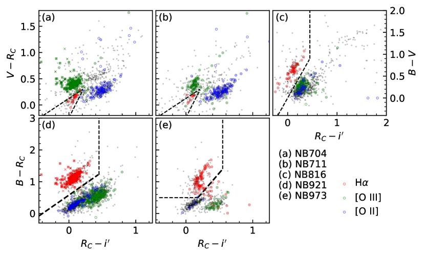
Figure 13: Two color selection of H$\alpha$ excess emitters in (a) NB704, (b) NB711, (c) NB816, (d) NB921, and (e) NB973 filters. The $x$ axes illustrate the $R_{\rm C}-i^{\prime}$ colors while the $y$ axes illustrate $V-R_{\rm C}$ (NB704, and NB711), $B-V$ (NB816), and $B-R_{\rm C}$ (NB921 and NB973). Galaxies with spectroscopic confirmation are indicated with open circles with colors indicating NB emission line: H$\alpha$ (red), [O iii]$\lambda$5007+H$\beta$ (green), and [O ii]$\lambda$3726,3728 (blue). In addition, dual NB704+NB921 emitters are overlaid as crosses, which occurs for two reasons: (1) [O iii]$\lambda$5007 and H$\alpha$ (red crosses), and (2) [O ii]$\lambda$3726,3728 and H$\beta$ (blue crosses), in NB704 and NB921 filters, respectively.

These color selections are illustrated in Figure 13(a)–(e) where spectroscopic samples are overlaid. From the sample of 7,963 emission-line galaxies, 962 of them were identified as H$\alpha$ emitting galaxies in the NB filters. However, nine sources identified as H$\alpha$ NB excess emitters have been excluded from the analysis, further reducing our sample to 953 galaxies. Among these nine galaxies, four galaxies were identified as active galactic nuclei (AGN) candidates, as they have [N ii]$\lambda 6583$/H$\alpha$ values above 0.54 (see Figure 1), the maximum value for star-forming galaxies (Kennicutt et al., 2008). One color-selected H$\alpha$ NB921 emitter had an excess emission in the IA598 (Nagao et al., 2008), an intermediate band filter, which we suspect is due to Ly$\alpha$ based on broad-band color information (the NB921 excess is likely due to [C iii]$\lambda\lambda$1907,1909). A color-selected H$\alpha$ NB816 excess emitter was excluded from the analysis because it had a photometric redshift from eazy (Brammer et al., 2008) suggesting that it may be a high-$z$ galaxy at $z\approx 3$. Another galaxy was excluded because its detection was too faint for its NB excess flux to be accurately obtained. The remaining two galaxies are identified by broad-band colors as H$\alpha$ NB704 emitters. However, they are also emitters in the NB973 filter; the NB704–NB973 combination for these two galaxies suggests that they are likely H$\beta$ NB704 and [S ii]$\lambda\lambda$6717,6731 NB973 emitters at $z\approx 0.45$.

Sources that were identified as H$\alpha$ emitters in the NB704 and/or NB711 filters were all assigned to a combined NB704+NB711 bin as they had similar redshifts, and combining the filters also increased sample sizes for stacking (see Section 3.2). Sources that were initially identified as dual H$\alpha$ emitters in the NB704 and NB921 filters were assigned to the NB921 filter since follow-up spectroscopy indicated that these instances occurred most likely due to [O iii] and H$\alpha$ emission in the NB704 and NB921 filters, respectively. Finally, one galaxy that was identified as a dual H$\alpha$ emitter in the NB816 and NB921 filter was placed in the NB921 bin upon inspection of the photometric detection.

A summary of the redshift ranges of H$\alpha$ emitting galaxies for each NB filter, as well as the NB filter properties, is available in Table 1. Table 2 shows more specific details for spectroscopically confirmed cases with MMT and Keck spectra. Spectroscopically confirmed Keck detections in the NB816 filter are not included in the analysis as they do not have H$\beta$ emission-line coverage.

Table 2: Summary of MMT and Keck spectroscopy

Filter	$N_{\rm H\alpha}$	$N_{\rm tgt}$	$N_{\rm spec}$	MMT				Keck
				$N_{\rm tgt}$	$N_{\rm spec}$	$z_{\rm spec}$		$N_{\rm tgt}$	$N_{\rm spec}$	$z_{\rm spec}$
(1)	(2)	(3)	(4)	(5)	(6)	(7)		(8)	(9)	(10)
NB704	89	31	21	28	21	0.068–0.078		…	…	…
NB711	50	7	3	7	3	0.085–0.091		…	…	…
NB816	191	63	49	61	49	0.229–0.252		…	…	…
NB921	390	222	206	192	180a	0.389–0.413		96	92	0.389–0.428
NB973	233	98	88	70	65	0.453–0.498		57	52	0.458–0.498

• (1): NB filter. (2): H$\alpha$ sample size, $N_{\rm H\alpha}$. (3): Spectroscopic targeted sample from MMT and/or Keck, $N_{\rm tgt}$. (4): Spectroscopic sample with redshift determination from MMT and/or Keck, $N_{\rm spec}$. (5)–(7): $N_{\rm tgt}$, $N_{\rm spec}$ and $z_{\rm spec}$ range for MMT. (8)–(10): $N_{\rm tgt}$, $N_{\rm spec}$ and $z_{\rm spec}$ range for Keck. Note that there are merged detections which were targeted by both MMT and Keck.

• 154 of 180 H$\alpha$ NB921 emitters had their MMT H$\alpha$ measurements excluded (due to poor sky subtraction, flux calibration, and/or being too close to the spectral coverage limit, 9200Å).

3.2 Spectral Stacking Procedure

The main goal of this study is to derive dust-corrected H$\alpha$-based SFRs from NB photometry. This measurement requires that we correct the NB photometry for [N ii] emission and dust attenuation (discussed later in Sections 4.1.2 and 4.1.3, respectively). While these corrections can be derived from measurements on individual galaxies, only 158 of the 953 H$\alpha$ emitting galaxies have emission line measurements reliable enough to obtain corrections. Therefore, in order to derive average corrections for the remainder of the galaxies in our sample, we construct composite spectra from stacking the MMT and Keck spectra.

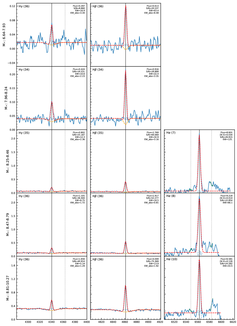
Figure 14: Composite spectra for the MMT NB921 sample (solid blue) with the best-fitting Gaussian profile (dashed red) and the RMS (dashed light blue). For the left and middle panels, the best-fitting Balmer absorption Gaussian profile is overlaid as well (dashed orange). This sample is split into five $M_{\star}$ bins. The $x$-axis is rest-frame wavelength in units of Å and the $y$-axis is flux density in units of 10^-17 erg s^-1 cm^-2 Å^-1. [N ii]$\lambda\lambda$6548,6583 lines are denoted by the vertical dotted lines in the right-most panels. “[N ii]” in the upper right legend denotes the emission-line flux ratio of [N ii]$\lambda$6583 to H$\alpha$. [O iii]$\lambda$4363 lines are denoted by the vertical dotted lines in the left-most panels.

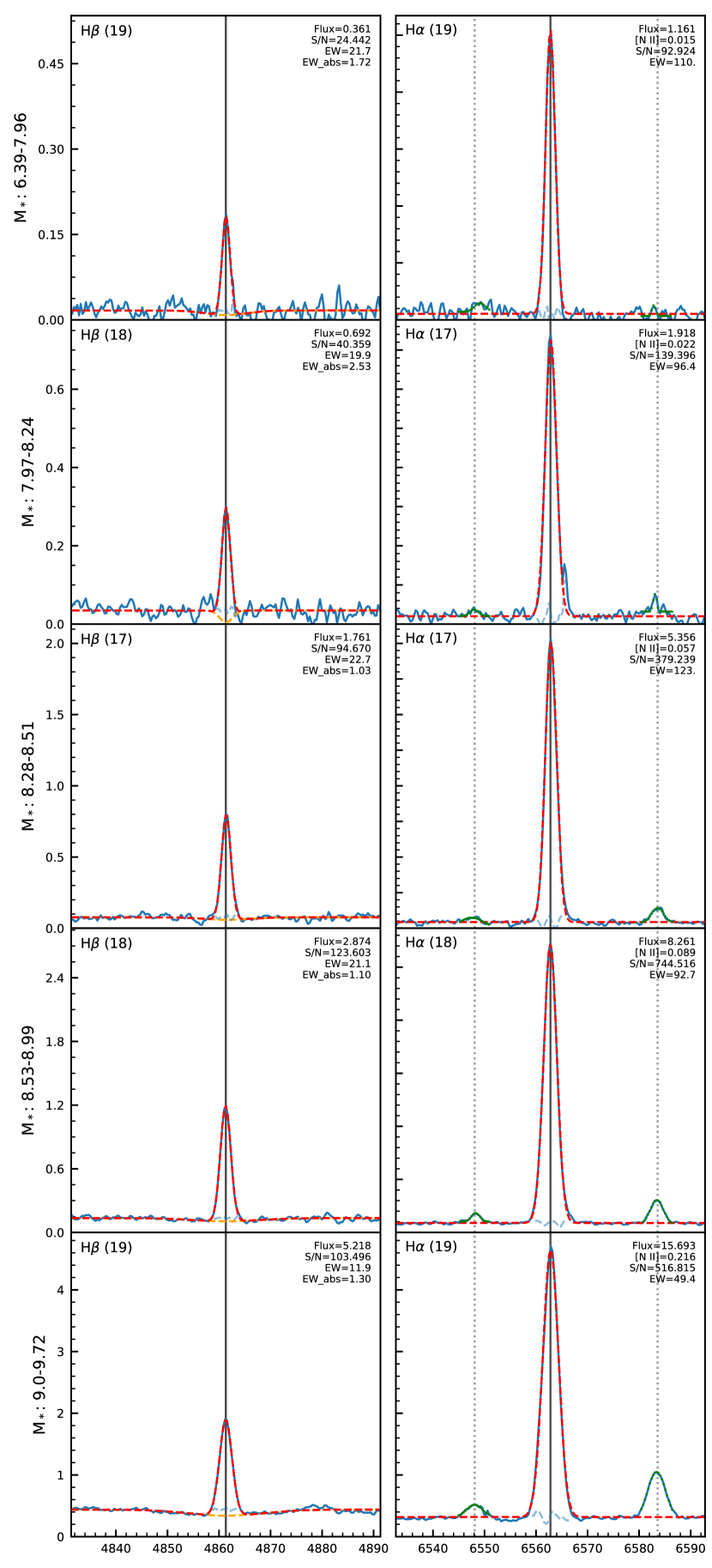
Figure 15: Similar to Figure 14, but for the Keck NB921 sample.

There were 318 galaxies with spectroscopic redshift determination from MMT and 144 from Keck, and 94 of those galaxies have redshift determination from joint spectroscopy. Of the galaxies with spectroscopic redshift determination, 315 have full H$\gamma$ emission-line coverage from MMT and 143 have full H$\beta$ emission-line coverage from Keck, with 91 having redshift determination from joint spectroscopy. The spectra for these galaxies were initially stacked in separate subsamples of redshift ($z$) and $M_{\star}$. Based on the quality of the stacks (high signal-to-noise and large numbers of spectra in each bin), finer stacking was done—a combination of $M_{\star}$ and redshift (hereafter $M_{\star}$–$z$; see Figure 14 for MMT, Figure 15 for Keck).

For the $M_{\star}$–$z$ binning, each galaxy was assigned a $z$ bin according to its corresponding narrowband filter bin (NB704+NB711, NB816, NB921, or NB973 for MMT; NB921 or NB973 for Keck). Then, depending on how many galaxies were in the $z$ bin, each galaxy was further binned into $M_{\star}$ bins. At least two $M_{\star}$ sub-bins and no more than five $M_{\star}$ sub-bins were required. This resulted in at least nine sources per $M_{\star}$–$z$ bin.

The spectral stacking procedure was as follows. First, the spectrum of each galaxy was shifted to the rest-frame and interpolated to a proper rest-frame wavelength grid. We then constructed average spectra and fitted the resulting composite spectra with Gaussian profiles. The H$\gamma$ and H$\beta$ lines were fit using double Gaussian line profiles, each with one positive and one negative component, to accurately account for Balmer stellar absorption near the centre of the emission lines. The H$\alpha$ line was fit using a single positive Gaussian function. The [N ii]$\lambda\lambda$6548,6583 emission lines near the H$\alpha$ lines were also fit in order to correct the NB excess flux measurements for contamination from the [N ii] lines (see Section 4.1.2). In the $M_{\star}$–$z$ stacks, the [N ii]/H$\alpha$ flux ratio, a metallicity indicator, increases as expected with increasing stellar mass (i.e., the mass–metallicity relation; Erb et al., 2006). All fits were done using the scipy.optimize.curve_fit routine (version 1.0.1) in Python (version 3.7.3). From these Gaussian profiles, we derive line fluxes, equivalent widths, and flux ratios for the composite spectra (provided in Tables 6 and 7).

4 Derived properties

This study focuses on the relationship between the H$\alpha$ SFR and stellar mass. These measurements are discussed in Sections 4.1 and 4.2, respectively.

4.1 H$\alpha$-based SFRs

In this study, we use H$\alpha$ luminosities to derive SFRs over other SFR indicators (e.g., UV+IR). There are a few reasons why the H$\alpha$ luminosity is more robust for our study. First, H$\alpha$ directly traces high mass star formation, as it is a recombination line arising from the ionizing radiation produced by short-lived OB stars. Second, for low-luminosity or low-mass galaxies, individual measurements of UV and infrared are either difficult or not feasible. Third, with H$\alpha$ probing a short time-scale ($\lesssim$5 Myr) for star formation, the dispersion of the SFR–$M_{\star}$ relation is more accurately measured.

To obtain dust-corrected H$\alpha$-based SFR measurements, we use emission-line fluxes/luminosities derived from NB excess photometry:

$$F_{\rm NB}=\Delta_{\rm NB}\frac{f_{\rm NB}-f_{\rm BB}}{1-(\Delta_{\rm NB}/\Delta_{\rm BB})},~{}{\rm and}$$ (5)

$$L_{\rm NB}=4\pi d_{L}^{2}F_{\rm NB},$$

where $f_{X}$ is the flux density in erg s^-1 cm^-2 Å^-1 for the relevant band, $\Delta$ is the FWHM of the wave band, and $d_{L}$ is the luminosity distance. For $\Delta$, the NB filter widths are reported in Table 1, and the broad-band filter widths are $\Delta R_{\rm C}$ = 1110 Å for NB704/NB711, $\Delta i^{\prime}$ = 1419 Å for NB816, and $\Delta z^{\prime}$ = 955 Å for NB921/NB973. For $d_{L}$, we either use the spectroscopic redshift (where available) or the central redshift of the NB filter: $z=0.074$, 0.086, 0.242, 0.401, and 0.486 for NB704, NB711, NB816, NB921, and NB973, respectively. For dual NB704+NB711 H$\alpha$ emitters, we use the NB704 measurements since spectroscopy suggests that H$\alpha$ is more accurately captured by the NB704 filter than by the NB711 filter. These NB measurements require three types of corrections to determine H$\alpha$ SFRs: (1) NB filter profile, (2) [N ii] contamination, and (3) dust attenuation.

4.1.1 NB filter profile correction

The NB filter profiles are not flat, and thus the NB excess fluxes or luminosities will depend on the location of the H$\alpha$ emission line within the filter:

$$L_{[\textsc{N~{}ii}]+{\rm H}\alpha}=f_{\rm filt}L_{\rm NB}.$$ (6)

To correct for this effect, we use spectroscopic redshifts to determine the necessary correction relative to the centre of the filter. For excess emitters with spectroscopic redshift, the average (median) NB filter corrections $f_{\rm filt}$ for NB704, NB711, NB816, NB921, and NB973 emitters are 1.08 (1.03), 1.28 (1.07), 1.49 (1.20), 1.13 (1.02), and 1.33 (1.09), respectively. For galaxies without spectroscopic redshifts, we use a fixed statistical correction of 1.29, 1.41, 1.29, 1.33, and 1.30, respectively. These statistical corrections are derived from a weighted average based on the filter profiles.

The discrepancies between the average (median) corrections and the fixed statistical corrections likely have a number of possible reasons. First, many galaxies with spectroscopic follow-up tend to fall closer to the centre of the NB filter profile. Second, selection bias effects may have skewed the redshift distribution towards a narrower one, as NB704 and NB921 dual emitters were targeted more often (higher spectroscopic completeness for two different samples). Third, cosmic variance may have also skewed our distribution, as spectroscopic follow-up (especially in NB921 and NB973 emitters) occurred within a small field of view. Finally, for some cases (e.g., the sample of NB704 or NB9711 emitters), we do not have many spectra, so outliers may heavily influence the redshift distribution of the spectroscopic sample.

4.1.2 [N ii] correction

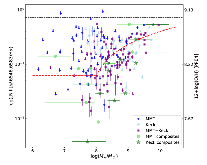
Figure 1: The flux ratio of [N ii]$\lambda\lambda$6548,6583 to H$\alpha$ as a function of stellar mass. Since [N ii]$\lambda$6548 is often undetected, we adopt [N ii]$\lambda 6583$/$\lambda 6548$ = 2.96 (Osterbrock & Ferland, 2006). Arrows indicate upper flux limits for individual galaxies with S/N $<2$ on [N ii]$\lambda 6583$. Horizontal bars indicate the mass range of the composite stacks. The dashed red line indicates the piecewise fit between the [N ii]/H$\alpha$ flux ratio and $M_{\star}$ (Equation 7). The dashed black line indicates the maximum value of [N ii]$\lambda 6583$/H$\alpha$ = 0.54 above which galaxies are likely AGNs instead of star-forming galaxies (Kennicutt et al., 2008).

The NB filters are wide enough ($\sim$100 Å) to include [N ii]$\lambda\lambda$6548,6583 emission (hereafter [N ii]). To correct for this contribution, we use emission-line measurements from individual galaxies (S/N $\geq 2$ on [N ii]$\lambda 6583$) and average measurements from composite spectra (see Section 3.2). The composite spectra used to apply these corrections consist of measurements from Keck $M_{\star}$–$z$ stacks, and measurements from MMT $M_{\star}$–$z$ stacks where Keck measurements are not available (e.g., sources detected in just the NB704, NB711, NB816 filters). We illustrate these [N ii] measurements in Figure 1. For the composite spectra, a least-squares fit was determined between the [N ii]/H$\alpha$ flux ratio and $M_{\star}$. This least-squares fit, also illustrated in Figure 1, is described as:

$$\frac{[\textsc{N~{}ii}]}{{\rm H}\alpha}=0.062~{}(x\leq 8.0),~{}{\rm and}$$ (7)

$$\frac{[\textsc{N~{}ii}]}{{\rm H}\alpha}=0.169x-1.293~{}(x>8.0),$$

where $x\equiv\log(M_{\star}/M_{\odot})$. Since [N ii]$\lambda$6548 is weak, we assume a flux ratio of $\lambda$6583/$\lambda$6548 = 2.96 (Osterbrock & Ferland, 2006). Thus, the observed H$\alpha$ luminosity is:

$$L_{{\rm H}\alpha}=\frac{1}{1+[\textsc{N~{}ii}]/{\rm H}\alpha}L_{[\textsc{N~{}ii}]+{\rm H}\alpha}.$$ (8)

4.1.3 Dust attenuation correction from Balmer decrements

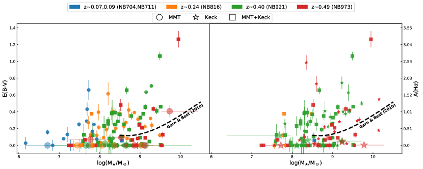
Figure 2: Dust attenuation color excess derived from Balmer decrements for individual sources (small filled shapes) and composite $M_{\star}$–$z$ stacks (large transparent shapes). The H$\alpha$/H$\beta$ Balmer decrements are plotted where they exist; otherwise the H$\gamma$/H$\beta$ Balmer decrements are plotted. Measurements from MMT, Keck, and a combination of both are indicated as circles, stars and squares, respectively. The relationship between $E$($B$–$V$) and stellar mass for local galaxies (Garn & Best, 2010) is illustrated by the black dashed line.

The “gold standard” of dust attenuation correction is the use of Balmer decrements, the H$\alpha$/H$\beta$ and H$\gamma$/H$\beta$ flux ratios from spectroscopic measurements (Osterbrock & Ferland, 2006; Kennicutt & Evans, 2012). The advantage here is that the Balmer decrements trace the dust associated with the source of H$\alpha$ emission, the ionized gas. Our sample has deep spectroscopy for $\approx$34% of the H$\alpha$ emitting sample, and reliable individual Balmer line measurements for $\approx$11% of the sample. Through stacked measurements of emission lines from galaxies with spectroscopic coverage (Section 3.2), we are able to use Balmer decrements to determine dust attenuation corrections for the entire sample. Here, the color excess $E$($B$–$V$) for nebular gas and amount of attenuation at H$\alpha$ are given by

$$\log\left[\frac{({\rm H}n/{\rm H}\beta)_{\rm obs}}{({\rm H}n/{\rm H}\beta)_{0}}\right]=-0.4E(B-V)[k({\rm H}n)-k({\rm H}\beta)],{\rm~{}and}$$ (9)

$$A({\rm H}\alpha)\equiv k({\rm H}\alpha)E(B-V),$$

where H$n$ is either H$\alpha$ or H$\gamma$, $k$(H$n$) is the attenuation coefficient following Cardelli et al. (1989), and the intrinsic Balmer decrements are (H$\alpha$/H$\beta$)${}_{0}=2.86$ and (H$\gamma$/H$\beta$)${}_{0}=0.468$ assuming Case B recombination with an electron temperature of 10⁴ K.

We illustrate $E(B-V)$ and $A({\rm H}\alpha)$ for individual galaxies and for composite stacks in Figure 2. Here, Balmer decrement values from the composite $M_{\star}$–$z$ spectra are used as they most accurately describe what the average dust attenuation is as a function of stellar mass and redshift. The majority of the individual sources have significantly higher $E$($B$–$V$) values than predicted by the empirical $E$($B$–$V$)–$M_{\star}$ relation for local galaxies (Garn & Best, 2010), indicating that adopting this local relation is not ideal for our sample.

For galaxies without spectra or with less reliable detections of the Balmer lines, we use the composite measurements as follows. For NB704, NB711 and NB816 H$\alpha$ emitters, we use the corresponding H$\alpha$/H$\beta$ Balmer decrement from the MMT $M_{\star}$–$z$ composites. For NB921 H$\alpha$ emitters, we use the Keck (MMT) H$\alpha$/H$\beta$ Balmer decrements for stellar masses of $M_{\star}\lesssim 5\times 10^{9}$ ($M_{\star}\gtrsim 5\times 10^{9}$) $M_{\odot}$. Finally for NB973 H$\alpha$ emitters, we use the Keck H$\alpha$/H$\beta$ Balmer decrements. After applying the dust attenuation corrections, the dust-corrected H$\alpha$ luminosity is:

$$\log\left(L_{{\rm H}\alpha,{\rm corr}}\right)=\log\left(L_{{\rm H}\alpha}\right)+0.4A({\rm H}\alpha).$$ (10)

4.1.4 Deriving SFRs

Assuming a Chabrier (2003) initial mass function (IMF) with minimum and maximum masses of 0.1 and 100 $M_{\odot}$ and solar metallicity (Kennicutt, 1998), the SFR can be estimated from the dust-corrected H$\alpha$ luminosity as

$$\frac{{\rm SFR}}{M_{\odot}\ {\rm yr}^{-1}}=4.4\times 10^{-42}\cdot\frac{L_{{\rm H}\alpha,\rm corr}}{{\rm erg}~{}{\rm s}^{-1}}.$$ (11)

However, the majority of our galaxies are at low stellar masses, which suggests that they have low metal abundances. Following Ly et al. (2016), we use a metallicity-dependent SFR–$L$(H$\alpha$) conversion:

$$\log\left[\frac{{\rm SFR}(M_{\odot}\ {\rm yr}^{-1})}{L_{{\rm H}\alpha,\rm corr}({\rm erg}~{}{\rm s}^{-1})}\right]=-41.34+0.39y+0.127y^{2},$$ (12)

where $y=\log({\rm O/H})+3.31.$ This relation was determined using H$\alpha$ luminosity predictions from Starburst99 spectral synthesis models (Leitherer et al., 1999). Here, we adopt the Padova stellar tracks (Bressan et al., 1993; Fagotto et al., 1994), a constant star formation history, and metallicities of 0.02, 0.20, 0.40, 1.0, and 2.5 $Z_{\sun}$. The original estimates were based on a Kroupa (2001) IMF, and were transformed to a Chabrier (2003) IMF with an offset of 0.1 dex. This relation is valid between 0.02$Z_{\sun}$ and 2.5$Z_{\sun}$ or $12+\log({\rm O/H})=7.0$ and 9.1, and thus is applicable to our entire sample. To estimate the oxygen abundances for our galaxies, we use the [N ii]$\lambda$6583/H$\alpha$ flux ratio either from individual or composite measurements (see Figure 1). Specifically, we use the Pettini & Pagel (2004) cubic calibration.

After correcting for the NB filter profile, [N ii] contamination, and dust attenuation, the 953 identified H$\alpha$ emitting NB excess galaxies have SFRs ranging between $10^{-3.57}M_{\odot}\ {\rm yr}^{-1}$ to $10^{1.40}M_{\odot}\ {\rm yr}^{-1}$ (mean: $10^{-1.46}M_{\odot}\ {\rm yr}^{-1}$).

4.2 Stellar masses from SED modeling

The Fitting and Assessment of Synthetic Templates (FAST; Kriek et al., 2009) code was used to determine physical properties of the full NB excess emitter sample by modeling their optical-to-infrared SEDs. FAST fits the broadband photometric data points with modeled fluxes from stellar synthesis models. In our SED modeling, we use either spectroscopic redshifts or central redshifts for the relevant NB filter (see Table 1). Photometric data are obtained from running SExtractor (version 2.5.0; Bertin & Arnouts, 1996) with NB images for source detection. These galaxies have also been imaged in the FUV and NUV bands with GALEX (Martin et al., 2005); for these measurements, more accurate photometry is obtained by point spread function fitting with iraf/daophot (version 2.16; Stetson, 1987). Further GALEX imaging and photometric measurement details are available in Ly et al. (2009), Ly et al. (2011a), and Ly et al. (2016).

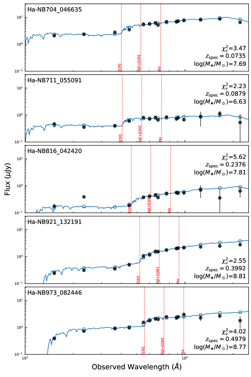
Figure 3: SEDs (grey filled circles) and the best-fitting results from modeling the SED (solid blue line and open blue circles) in each of the five NB filters. These SEDs were randomly selected. Vertical red dashed lines illustrate the location of common spectral features. Good agreement is seen between photometric and modeled fluxes.

In FAST, Bruzual & Charlot (2003) stellar synthesis models, with an exponentially declining star formation history, SFR $\propto$ $\exp(-t/\tau)$, were used. We chose $\log(\tau/{\rm yr})$ = 7.0, 8.0, 9.0, and 10.0 in order to include bursty, intermediate, and roughly constant star formation histories. The Calzetti et al. (2000) dust attenuation relation was adopted, and we assumed a Chabrier (2003) initial mass function (IMF) and a stellar metallicity of $Z=0.02$.

The grid of models FAST considered also included dust reddening ($A_{V}$) at 0.0–3.0 mag in 0.1 mag increments, stellar ages of $\log({\rm age/yr})=7.0$–10.1 in 0.1 dex increments, and redshifts from 0.01–1.70 in 0.001 increments. Some of the physical properties that were determined include best-fitting stellar ages, $A_{V}$, SFR, stellar masses, and $\tau$ values, as well as their respective confidence intervals. These estimates were determined from $\chi^{2}$ minimization; FAST determines every point of the model grid.

A sample of SED fits, for each NB sample, can be seen in Figure 3. The SED models fit the data points well within error bars. Identified H$\alpha$ emitting NB excess galaxies have stellar masses between $10^{4.3}$ to $10^{10.4}~{}M_{\odot}$ (mean: $10^{7.96}~{}M_{\odot}$). Galaxies corresponding to the low end of these stellar masses were ultimately not included in our analysis (Section 5 for discussion).

5 Results & Discussion

We discuss four key results from our study: comparison between UV and H$\alpha$ SFRs (Section 5.1), the H$\alpha$ specific SFR and its evolution with redshift and dependence with stellar mass (Section 5.2), the SFR–$M_{\star}$ relation (Section 5.3), and the dispersion of the SFR–$M_{\star}$ relation (Section 5.4). We also examine the completeness of our survey in Section 5.5.

The following results and analyses required that we further restrict our sample for the following reasons. First, due to a large amount of galaxies detected near the 3$\sigma$ flux limit, a higher sigma selection (4$\sigma$) was imposed on NB excess fluxes. The new selection reduces the sample to 730 galaxies. The revised 4$\sigma$ NB excess flux selections correspond to $7.3\times 10^{-18}$ (NB704), $8.4\times 10^{-18}$ (NB711), $5.9\times 10^{-18}$ (NB816), $7.8\times 10^{-18}$ (NB921), and ${2.3\times 10^{-16}}$ erg s^-1 cm^-2 (NB973).

Additionally, we impose a low-mass cutoff of $10^{6}M_{\odot}$ as none of the galaxies below this cutoff were spectroscopically confirmed, and many of them had unreliable photometric redshifts from eazy. In fact, a number of these low-mass galaxies had photometric redshifts suggestive of different emission lines corresponding to higher redshifts and hence higher stellar masses. This new selection, with both the 4$\sigma$ cut and the low-mass limit cutoff of $10^{6}M_{\odot}$, reduces the sample to 714 galaxies.

In our analyses, we randomise each data point in our observations 10,000 times, assuming a Gaussian with the standard deviation equal to the measurement uncertainty. Each randomization is re-fit with scipy.optimize.curve_fit. Uncertainties for reported averages are derived using the bootstrap approach, where we randomly select galaxies and compute the average 10,000 times. Randomization accounts for measurement uncertainties, examines degeneracies in our fitting parameters, and minimizes the number of underlying assumptions that are adopted.

5.1 Comparisons between H$\alpha$ and UV SFRs

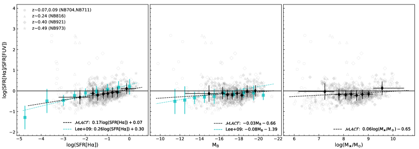
Figure 4: Ratio of observed H$\alpha$-to-FUV SFR against the H$\alpha$ SFR (left panel), B-band absolute magnitude (middle panel), and stellar mass (right panel). Empty (filled) symbols represent galaxies without (with) spectroscopic confirmation. Average values in each 12.5-percentile bin of galaxies with spectroscopic confirmation are represented with solid black diamonds, with 1$\sigma$ scatter plotted as well. A linear least squares fit to the data is overlaid with a dashed black line, with the best-fitting line for each dataset given in the lower right of each panel. For the first two panels, data and results from Lee et al. (2009) are plotted in cyan. A Chabrier (2003) IMF is adopted here.

In addition to H$\alpha$-derived SFRs, our photometric data provide FUV continuum measurements, allowing us to compare two independent SFR estimates. Under the assumption of a continuous star formation history, these two SFR measurements, which probe different time-scale ($\lesssim$5 Myr for H$\alpha$ and $\lesssim$100 Myr for FUV), should agree. However, for low-SFR galaxies, a systematic discrepancy between H$\alpha$- and FUV-derived SFRs has been observed, wherein the H$\alpha$ indicator underpredicts the total SFR compared to the FUV (e.g., Lee et al., 2009). One explanation of this discrepancy is that, at low SFRs, statistically sampling the IMF will not produce enough massive OB stars, resulting in a deficit for H$\alpha$ measurements (Weidner et al., 2013).

To derive UV SFRs, we follow Section 4.1.4 where we use the following metallicity-dependent $L$(FUV)–SFR relation derived from Starburst99 estimates:

$$\log\left[\frac{{\rm SFR}(M_{\odot}\ {\rm yr}^{-1})}{L_{\nu}(1500)({\rm erg}~{}{\rm s}^{-1}~{}{\rm Hz}^{-1})}\right]=-28.179+0.151y+0.053y^{2}.$$ (13)

Here we also adopt a Chabrier (2003) IMF with minimum and maximum masses of 0.1 and 100 $M_{\odot}$. The 1500Å luminosities were obtained from interpolating our best-fitting SEDs derived from our FAST modeling (see Section 4.2).

Under the assumption that the FUV luminosity is a more robust indicator of star formation in low-mass galaxies than H$\alpha$, we can systematically correct our H$\alpha$ SFRs. For robustness, we only consider galaxies with spectroscopic confirmation. As demonstrated in Figure 4, the observed H$\alpha$-to-FUV SFR ratio shows a deficit against the H$\alpha$ SFR, B-band absolute magnitude, and stellar mass. This deficit can be described as follows:

$$\log\left(\frac{{\rm SFR[H\alpha]}}{{\rm SFR[FUV]}}\right)=0.17\psi+0.07,$$ (14)

where $\psi\equiv\log({\rm SFR[H\alpha]})$. Correcting our SFRs for dust attenuation, which is illustrated in Figure 5, we find good agreement with Lee et al. (2009). Our values of observed and dust-corrected H$\alpha$-to-FUV SFR ratios against the H$\alpha$ SFRs, per 12.5-percentile bin of galaxies, are tabulated in Table 3.

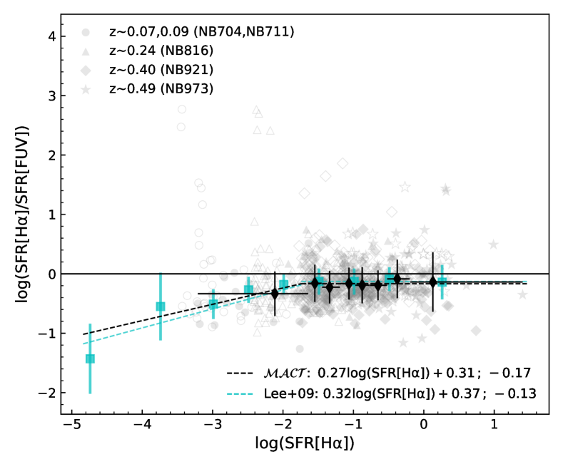
Figure 5: Similar to the left panel of Figure 4, but for dust-corrected SFRs. A piecewise fit to the data is overlaid with a black dashed line and labelled in the lower right corner. The form of the fit is a linear relation for log(SFR[H$\alpha$]) $\leq-1.74$, and a constant at higher SFR. Good agreement is seen with respect to Lee et al. (2009).

Table 3: Summary of UV–H$\alpha$ SFR comparisons

$\log{\left({\rm SFR[H\alpha]}\right)}$	$N_{\rm spec}$	$\log\left(\frac{{\rm SFR[H\alpha]}}{{\rm SFR[FUV]}}\right)$
(1)	(2)	(3)
Observed
–2.24${}_{-0.97}^{+0.46}$	45	–0.31${}_{-0.55}^{+0.89}$
–1.65${}_{-0.12}^{+0.10}$	44	–0.12${}_{-0.50}^{+0.72}$
–1.43${}_{-0.11}^{+0.12}$	44	–0.21${}_{-0.41}^{+0.87}$
–1.18${}_{-0.10}^{+0.10}$	45	–0.15${}_{-0.53}^{+0.54}$
–0.98${}_{-0.10}^{+0.09}$	44	–0.13${}_{-0.44}^{+0.44}$
–0.77${}_{-0.11}^{+0.10}$	44	–0.08${}_{-0.41}^{+0.70}$
–0.54${}_{-0.13}^{+0.15}$	44	–0.07${}_{-0.46}^{+0.83}$
–0.12${}_{-0.26}^{+0.43}$	45	+0.11${}_{-0.38}^{+0.74}$
Dust-corrected
–2.12${}_{-1.09}^{+0.47}$	45	–0.33${}_{-0.93}^{+1.08}$
–1.55${}_{-0.09}^{+0.10}$	44	–0.16${}_{-0.51}^{+0.74}$
–1.34${}_{-0.11}^{+0.15}$	44	–0.23${}_{-0.46}^{+0.80}$
–1.06${}_{-0.12}^{+0.09}$	45	–0.16${}_{-0.67}^{+0.50}$
–0.88${}_{-0.10}^{+0.10}$	44	–0.19${}_{-0.67}^{+0.94}$
–0.65${}_{-0.11}^{+0.13}$	44	–0.19${}_{-0.57}^{+0.70}$
–0.38${}_{-0.14}^{+0.18}$	44	–0.09${}_{-1.07}^{+0.77}$
+0.13${}_{-0.32}^{+1.27}$	45	–0.14${}_{-0.95}^{+1.57}$

• (1): The mean value of the logarithm of the H$\alpha$ SFR values per 12.5-percentile bin of galaxies. The range of the bin is denoted as errors. (2): Number of spectroscopic measurements. (3): The mean value of the logarithm of ratio of H$\alpha$-to-FUV SFRs. The 1$\sigma$ scatter is denoted as errors. Observed values are illustrated in the left-hand panel of Figure 4. Dust-corrected values are illustrated in Figure 5, with dust attenuation corrections based on Balmer decrements (see Section 4.1.3).

Our sample and the sample in Lee et al. (2009) were independently selected using different methods at different redshifts; the agreement between these studies supports the prediction in Lee et al. (2009) whereby the semi-empirical integrated galactic IMF model (Kroupa & Weidner, 2003) could account for the systemic underprediction of H$\alpha$-derived SFRs (Weidner et al., 2013). In the work of Lee et al. (2009), they fit a piece-wise function with turnover at –1.5. Following their approach, our resulting fit is:

$$\log\left(\frac{{\rm SFR[H\alpha]}}{{\rm SFR[FUV]}}\right)=0.27\psi+0.31~{}(\psi\leq-1.74),~{}{\rm and}$$ (15)

$$\log\left(\frac{{\rm SFR[H\alpha]}}{{\rm SFR[FUV]}}\right)=-0.17~{}(\psi>-1.74).$$

To correct for this underprediction, we use the best-fitting relation between the dust-corrected H$\alpha$-to-FUV SFR ratio and the H$\alpha$ SFR. The resulting “true” H$\alpha$ SFR is then:

$$\psi_{\rm true}=\psi-\log\left(\frac{{\rm SFR[H\alpha]}}{{\rm SFR[FUV]}}\right).$$ (16)

In our analyses below, we report results with the H$\alpha$ underprediction correction.

5.2 H$\alpha$ Specific SFRs

The SFR per unit stellar mass, or specific SFR (sSFR), is often used as an indicator of active star formation as it is related to the gas depletion time-scale (e.g., Kennicutt, 1998; Kennicutt & Evans, 2012). Studies have examined how sSFR evolves toward higher redshift below $z\lesssim 2$ (e.g., Lehnert et al., 2015; Tasca et al., 2015) and how it depends on stellar mass (e.g., Salim et al., 2007; de los Reyes et al., 2015; Davies et al., 2019). However, these studies mostly probe higher mass galaxies, and have not examined evolution of galaxies below stellar masses of 10${}^{9}M_{\odot}$.

To address this lack of understanding, we first use the $\mathcal{MACT}$ sample to determine the evolution of sSFR at a given stellar mass, $\log(M_{\star}/M_{\odot})=8.0\pm 0.5$. We selected this stellar mass for two reasons: (1) it is near the average stellar mass of the reduced $\mathcal{MACT}$ sample, $10^{8.3}~{}M_{\odot}$, and (2) all NB redshift bins, from $z=0.07$ to 0.5, are included in this analysis. We explore two redshift dependencies and find significant evolution: $\log({\rm sSFR})\propto A\log(1+z)$ with $A=5.26\pm 0.75$, and $\log({\rm sSFR})\propto Bz$ with $B=1.83\pm 0.26$. This result is consistent with the previously mentioned studies of higher mass galaxies that have found, at fixed stellar mass, increased sSFR evolution toward higher redshift over our redshift range.

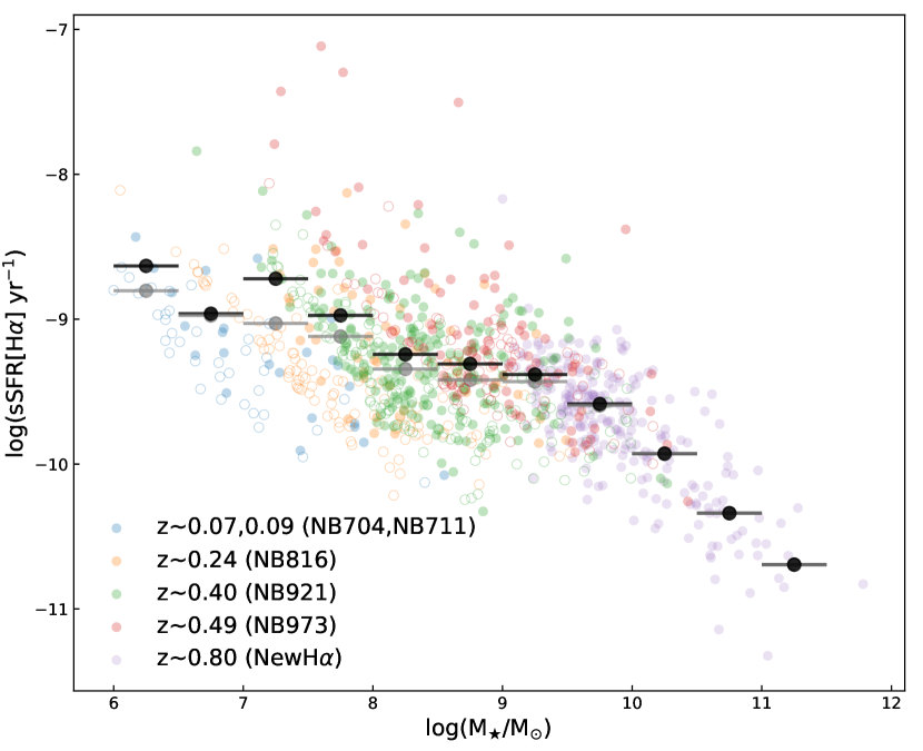
Figure 6: Specific SFRs of NB-selected H$\alpha$ galaxies as a function of stellar mass, spanning six dex in stellar mass and half the age of the Universe (up to $z\approx 0.8$). Colored empty (filled) symbols represent galaxies without (with) spectroscopic confirmation. Gray (black) circles represent the average sSFR for all sources (sources with spectroscopic confirmation) in each stellar mass bin. This figure includes measurements from the NewH$\alpha$ survey (de los Reyes et al., 2015).

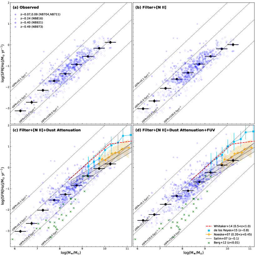
Figure 7: The SFR–$M_{\star}$ relation for H$\alpha$ emitters between $z=0.07$ and $z=0.5$. Empty (filled) symbols represent galaxies without (with) spectroscopic confirmation. (a) the observed sample without any applied corrections, and (b), (c), and (d) have different corrections applied, as indicated in the figure. Average SFRs in each stellar mass bin are represented with solid black dots. Results from other empirical studies are overlaid as follows: Whitaker et al. (2014) with dashed red lines, NewH$\alpha$ measurements from de los Reyes et al. (2015) with cyan squares, Noeske et al. (2007) with orange pluses, Salim et al. (2007) with a solid black line, and Berg et al. (2012) with green crosses.

Next, we examine the correlation of sSFR with stellar mass at $\lesssim 3\times 10^{9}M_{\odot}$, which is illustrated in Figure 6. Since our study is unable to probe high stellar masses ($\gtrsim 3\times 10^{9}M_{\odot}$), we include measurements from the NewH$\alpha$ survey (Ly et al., 2011a; Lee et al., 2012). The NewH$\alpha$ survey identified 394 H$\alpha$ emitting galaxies using a near-infrared NB filter in several deep fields for a total of 0.82 deg² with stellar masses of $3\times 10^{9}$–$10^{11}~{}M_{\odot}$. It probes higher redshifts ($z\approx 0.8$) down to an emission-line flux of ${2\times 10^{-17}}$ erg s^-1 cm^-2 (3$\sigma$) or an observed H$\alpha$ SFR of $0.3M_{\odot}$ yr^-1 at the low-luminosity end, and identified galaxies with a minimum H$\alpha$ rest-frame equivalent width (EW) of 22 Å at the high-mass end. These H$\alpha$-selected galaxies with spectroscopic confirmation (N = 299) are illustrated in Figure 6 in purple. Here we re-derived H$\alpha$ SFRs for the NewH$\alpha$ sample by using our metallicity-dependent SFR relation. To estimate metallicity, we used the tabulated [N ii]/H$\alpha$ ratio from de los Reyes et al. (2015).

With the combined $\mathcal{MACT}$ and NewH$\alpha$ datasets, we find: (1) low-mass galaxies have higher sSFRs than high-mass (${\gtrsim 3\times 10^{9}M_{\odot}}$) galaxies, and (2) the sSFRs appear to plateau for low-mass galaxies unlike high-mass galaxies where there is a strong negative dependence. While the sSFR–$M_{\star}$ relation flattens toward lower stellar masses, it is not entirely a constant. Thus, this result suggests that the SFR–$M_{\star}$ relation has a slope less than unity for most stellar masses. This result is consistent with many studies such as Salim et al. (2007) and Davies et al. (2019) for local Universe galaxies, McGaugh et al. (2017) for low surface brightness local galaxies, and Boogaard et al. (2018) for field star-forming galaxies (see Section 5.3.1). This trend is less evident for galaxies with spectroscopic confirmation, but we caution this may be a selection effect due to spectroscopic constraints of emission line detections. We note that these results are not due to an incompleteness of our study, as higher sSFR galaxies would have easily been detected with our narrowband photometry.

5.3 Star Formation Sequence Relation

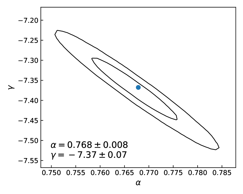
Figure 8: Confidence contours for linear regression fitting following a redshift-independent SFR–$M_{\star}$ relation (Equation 17).

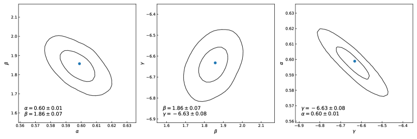
Figure 9: Similar to Figure 8, but fitting was performed with a redshift-dependent relation (Equation 18).

The SFR–$M_{\star}$ relation for our sample of 714 galaxies, with incremental corrections applied (see Section 4.1.1–4.1.3 and Section 5.1), is presented in Figure 7. We find the SFR–$M_{\star}$ relation holds down to our low-mass limit cutoff of $10^{6}M_{\odot}$, pushing the explored mass range to $\sim$1.5 dex below previous studies. (The dispersion is $\sigma\approx 0.3$ dex; see Section 5.4.) For comparison, results from various studies at $z\lesssim 1$ (Noeske et al., 2007; Salim et al., 2007; Berg et al., 2012; Whitaker et al., 2014; de los Reyes et al., 2015) are overlaid. At the high-mass end, our sample is consistent with Noeske et al. (2007) and with the relation of Salim et al. (2007). The sample from Berg et al. (2012) lies consistently below our sample, but this discrepancy may be due to the fact that their galaxies are low-luminosity galaxies in the local Universe, whereas our galaxies are field galaxies at low to intermediate redshifts. Our relation is below the relation of de los Reyes et al. (2015) and Whitaker et al. (2014). This discrepancy is likely due to higher sSFR for higher redshift galaxies.

We fit the H$\alpha$ SFR–$M_{\star}$ relation with three different formalisms. First, we consider a linear relation between mass and SFR:

$$\log{({\rm SFR})}=\alpha\log{(M_{\star}/M_{\odot})}+\gamma.$$ (17)

The confidence contours are illustrated in Figure 8, and the best fit is $\alpha=0.768\pm 0.008$ and $\gamma=-7.37\pm 0.07$, with average residuals of 0.30 dex.

Next, we consider a redshift-dependent relation. We explored various possible redshift-dependent relations, including linear and polynomial dependences on $z$, $(1+z)$, and $\log(1+z)$. Ultimately, we used:

$$\log{({\rm SFR})}=\alpha\log{(M_{\star}/M_{\odot})}+\beta z+\gamma.$$ (18)

In this formalism, the redshift dependence in this relation only shifts the normalization of the relationship, and the slope of the stellar mass dependence is fixed for all redshifts. Of the various redshift-dependent relations we explored, this relation had the lowest residuals (0.26 dex) across stellar mass and redshift, while also having the simplest form. This relation also had lower residuals than the linear, redshift-independent relation considered between mass and SFR. The best fit with this formalism gives $\alpha=0.60\pm 0.01$, $\beta=1.86\pm 0.07$, and $\gamma=-6.63\pm 0.08$. These fit parameters are illustrated in Figure 9 with 68% and 95% confidence contours. The redshift-dependent SFR–$M_{\star}$ relation is provided in Figure 10. The average mass and SFR values in each stellar mass and redshift bin, provided in Table 8, agree with the best-fitting redshift dependent model. Both results indicate a less than unity slope dependence of SFR on mass.

Some studies (e.g., Whitaker et al., 2014; Lee et al., 2015), have found evidence for a ‘turnover’ at some characteristic mass $M_{\rm char}$. Although their values of $M_{\rm char}\sim 10^{10}~{}M_{\odot}$ are at the high end of the mass range of our sample, we consider the possibility that there might be a second turnover point at a lower mass range in our sample. As such, we investigate whether a broken power law with redshift dependence gives a better fit:

$$\log({\rm SFR})=\alpha[\log(M_{\star}/M_{\rm char})]+\beta z+\gamma.$$ (19)

We find that the residuals from considering this broken power law model are similar to those found with the redshift-dependent relation in Equation 18. Given that the redshift-dependent relation has fewer parameters, we decide to use Equation 18 as our best-fitting model for the rest of our analysis.

5.3.1 Comparison against other low-mass SFR–$M_{\star}$ relations

While low-mass galaxy studies have generally been limited, there are two notable studies that do examine the SFR–$M_{\star}$ relation in this domain. First, McGaugh et al. (2017) examined the SFR–$M_{\star}$ relation for low surface brightness galaxies using H$\alpha$ measurements for SFR. They found that these $z\approx 0$ galaxies followed a SFR–$M_{\star}$ sequence that is nearly unity ($1.04\pm 0.06$), much steeper than for more massive star-forming galaxies. However, as discussed in Section 5.1, H$\alpha$ can systematically underpredict massive star formation. Using the UV–H$\alpha$ SFR relation of Lee et al. (2009), we find a shallower slope of $0.68\pm 0.05$. While this slope is higher than our result ($0.60\pm 0.01$), we note that McGaugh et al. (2017) adopted a Salpeter (1955) IMF in their H$\alpha$ SFR estimates instead of a Chabrier (2003). Given the difference in IMF, the $2\sigma$ offset is marginal.

Second, Boogaard et al. (2018) examined low-mass galaxies, $7\leq\log(M_{\star}/M_{\odot})\leq 10.5$, in the Hubble Deep Field using data from the MUSE (Multi Unit Spectroscopic Explorer; Bacon et al., 2010) instrument. They looked at 179 star-forming galaxies at redshift $0.11<z<0.91$ with H$\beta$ and H$\alpha$ emission lines (with high spectroscopic measurements), from which SFRs were determined. The SFR–$M_{\star}$ relation they found was $\alpha^{\prime}=0.83^{+0.07}_{-0.06}$ and $\beta^{\prime}=1.74^{+0.66}_{-0.68}$ for the functional form ${\log(\rm{SFR})\propto\alpha^{\prime}\log(M_{\star}/M_{\odot})+\beta^{\prime}\log(1+z)}$. Notably, their value of $\alpha^{\prime}=0.83$ significantly differs from our value of $\alpha=0.58$. However, there are a few differences in the way our analyses were conducted: (1) their value of $\alpha^{\prime}$ for their redshift-dependent relation spanned a redshift range beyond our own; (2) their high-$z$ sample was dominated by H$\beta$-selected galaxies; and (3) they also did not apply the UV correction as we did.

In order to more directly compare our results, we examine the 72 galaxies for $0.1<z\leq 0.5$ from Boogaard et al. (2018), and derive SFRs in a consistent manner. We find that our samples overlap significantly across the full stellar mass range. We note however, that the fitting methods used differ, and thus differences in the fitting results are expected.

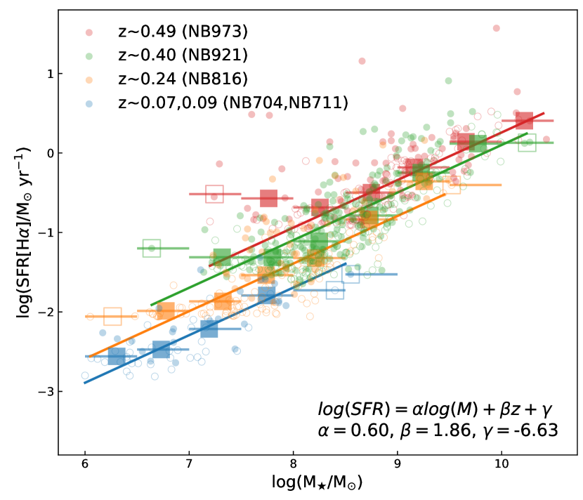
Figure 10: The SFR–$M_{\star}$ relation with the best fitting redshift-dependent functional form overlaid (solid lines; equation provided in the bottom right). Galaxies are represented by different colors depending on their redshift/NB filter. Empty (filled) circles represent galaxies without (with) spectroscopic confirmation. Squares represent the average SFRs and stellar masses of galaxies in each mass bin, with error bars representing the mass range. Open squares signify there are fewer than five galaxies.

5.4 Intrinsic Dispersion of the Star Formation Sequence Relation

The residuals of the SFR–$M_{\star}$ relation, illustrated in Figure 11, are obtained by differencing the dust-corrected SFR values against those predicted by the redshift-dependent SFR–$M_{\star}$ relation (Equation 18). The sample is divided into stellar mass bins, and the observed scatter is illustrated in this figure. Each mass bin also has an associated uncertainty due to systematics, which is derived from adding in quadrature the errors on the NB fluxes and on the $E$($B$–$V$) values. Subtracting in quadrature the systematic uncertainties from the observed scatter yields the estimated intrinsic dispersion as a function of mass for our SFR–$M_{\star}$ relation. These values are provided in Table 4.

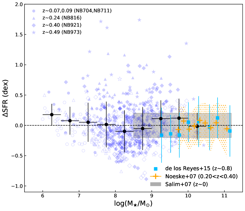
Figure 11: Deviations from the SFR–$M_{\star}$ relation (relative to the redshift-dependent SFR–$M_{\star}$ relation, Equation 18) for H$\alpha$ emitters between $z=0.07$ and $z=0.5$. Empty (filled) symbols represent galaxies without (with) spectroscopic confirmation. Vertical error bars for filled black circles illustrate the average dispersion in each bin, with horizontal error bars indicating the mass range. Results from other empirical studies are overlaid: de los Reyes et al. (2015) with cyan squares, Noeske et al. (2007) with orange pluses, and Salim et al. (2007) with a gray shaded region.

Over the stellar mass range of 10^7.0–10${}^{8.5}~{}M_{\odot}$, we observe that the intrinsic dispersion varies between $\approx$0.25–0.35 dex, with an average of $\approx$0.3 dex. The average intrinsic dispersion across the entire mass range is also $\approx$0.3 dex, suggesting there is no evolution of dispersion towards lower stellar masses. This result is aligned with similar intrinsic dispersion measures found in other studies probing higher mass ranges (e.g., Noeske et al., 2007; Whitaker et al., 2012b; Speagle et al., 2014; Schreiber et al., 2015).

Over similar stellar masses, our intrinsic dispersion is consistent with McGaugh et al. (2017), where they find $\sigma=0.34$ dex. However, our intrinsic dispersion of $\approx$0.3 dex differs from Boogaard et al. (2018), where they found an intrinsic dispersion of $0.44$ dex. One reason for the difference is that our study, as well as other studies mentioned above, are affected by the selection effects that miss low-sSFR galaxies. With our mock galaxy simulations (see Section 5.5), we find that the dispersion can be underestimated by a factor of $\approx$2 such that the SFR–$M_{\star}$ dispersion is $\approx$0.5 dex. Our simulations show a consistent dispersion across the stellar mass range 10⁶–10¹⁰ $M_{\odot}$, which suggests that there does not appear to be a significant evolution with stellar mass. The higher dispersion is consistent with local studies, such as Davies et al. (2019), where they find a dispersion of $\approx$0.4 dex above $3\times 10^{8}$ $M_{\odot}$ with a slow rise toward $\approx$0.6 dex at 10⁷ $M_{\odot}$.

Table 4: Summary of dispersion measurements from the SFR–$M_{\star}$ relation

$\log\left(\frac{M_{\star}}{M_{\odot}}\right)$	$\left<\log{\left(\frac{{\rm SFR}}{M_{\odot}/{\rm yr}}\right)}\right>$	$N$	$\sigma_{\rm obs}$	$\left<\sigma_{\rm sys}\right>$	$\left<\sigma_{\rm int}\right>$
(1)	(2)	(3)	(4)	(5)	(6)
6.0–6.5	–2.50 (–3.02)	18	0.178	0.247	…
6.5–7.0	–2.23 (–2.65)	29	0.230	0.197	0.119
7.0–7.5	–1.74 (–2.02)	68	0.322	0.202	0.251
7.5–8.0	–1.35 (–1.54)	127	0.378	0.190	0.326
8.0–8.5	–1.10 (–1.27)	170	0.347	0.143	0.316
8.5–9.0	–0.68 (–0.85)	164	0.354	0.112	0.336
9.0–9.5	–0.23 (–0.40)	88	0.302	0.053	0.297
9.5–10.0	+0.12 (–0.05)	42	0.322	0.035	0.320
10.0–10.5	+0.34 (+0.17)	8	0.222	0.024	0.220

• (1): Stellar mass range. (2): Average log SFR (average log SFR without FUV corrections). (3): Number of galaxies in each bin. (4)–(6): Observed scatter, average systematic uncertainties, and average intrinsic dispersion on the main sequence relation, respectively. These values are illustrated in Table 11.

5.5 Survey Selection and Completeness

The NB technique selects galaxies with (1) a minimum excess in the NB color (corresponding to a minimum observed emission-line EW) at the bright end; and (2) a 3$\sigma$ NB excess flux limit. These observable limits are provided in Table 5 for all five NB filters.

To understand the completeness of our study, we conduct Monte Carlo analyses where mock emission-line galaxies are created and selected through our NB criteria. This approach allows us to examine the selection effects across a number of observables including stellar mass, emission-line luminosity/flux, and emission-line EW. Our methodology is similar to Ly et al. (2011b) where we first adopt log-normal EW distributions, which are described by two quantities: the mean EW, $\left<\log{\rm EW}\right>$, and the dispersion, $\sigma[\log({\rm EW})]$. We chose a log-normal distribution because a number of studies have found that the H$\alpha$ emission-line EWs follow such a distribution (e.g., Lee et al., 2007).

For our Monte Carlo analysis, we consider a grid of $\left<\log{\rm EW}\right>$ and $\sigma[\log({\rm EW})]$ values, a total of 16 possibilities for each NB filter selection. In each simulation, we assign NB magnitudes for 5,000 modeled galaxies. The magnitudes of these sources are governed by the number counts obtained from the SDF NB SExtractor catalogs (Ly et al., 2007, 2012a, 2012b). By adopting a given log-normal EW distribution, a NB excess EW/color can be assigned to each mock galaxy. This ultimately populates the NB excess selection plot of NB excess color vs. NB magnitude (see Figure 12). For each modeled galaxy, we construct 100 randomizations with photometric uncertainties governed by limiting magnitudes for NB and broadband data. We then apply our NB color selections and identify which mock galaxies are selected. With mock photometry, we determine derived properties such as the emission-line flux and EW from the NB excess. We also apply corrections for the NB filter shape (see Section 4.1.1) and [N ii] contamination (see Section 4.1.2) to derive H$\alpha$ emission-line flux/luminosity and EW. To determine stellar masses for each mock galaxy, we construct an empirical relationship between broadband photometry and stellar mass estimates for our NB emitter samples. For simplicity, we use the broad-band filters that are used in our NB excess selection. We illustrate the derived properties of our mock galaxies in Figure 12.

With 16 possible log-normal EW distribution each with about 500,000 mock galaxies, and five NB filters, a total of 40 million galaxies were constructed to ensure that our simulations cover a wide range of possible priors. To determine which log-normal distribution represented the sample of emission-line galaxies selected in each filter, we compare the distributions of EW and line fluxes against what is measured from the observable samples. Here we normalise the mock distributions against the sample sizes for each filter, and computed reduced $\chi^{2}$ values. The best log-normal EW model for each NB filter was determined by using a weighted $\chi^{2}$ for both EW and line flux. In Table 5 we report the survey completeness at the 50% level for sSFR and SFR. Here the sSFR (SFR) completeness limit is at higher (lower) luminosities, where the minimum EW (NB 3$\sigma$ excess) determines our selection.

With these Monte Carlo simulations, we can determine how our adopted NB color selection impacts the SFR–$M_{\star}$ relation and our results. These color selections preferentially will miss low-mass low-SFR galaxies, which has two immediate effects on the SFR–$M_{\star}$ relation. First the slope can be flattened. Second, the amount of dispersion will be underestimated. We examine these effects in the following manner. We first compare the observed slope (after applying the NB selection) against the intrinsic slope, limiting our analysis to the best-fitting log-normal EW models that we describe above for each filter. We find that the slope is not significantly impacted. The slope will not be notably flattened because low-EW galaxies are not selected across all stellar masses.

For the dispersion, we (1) randomly select, from our mock samples, the number of $\mathcal{MACT}$ galaxies in each $M_{\star}$–$z$ bin, (2) compute the offset relative to the best-fitting SFR–$M_{\star}$ relation for each redshift, and then (3) combine the results of each NB filter to determine the standard deviation. We repeat this computation 1,000 times to estimate the range in dispersion, and then compare our results to the intrinsic dispersion, which is measured in the SFR–$M_{\star}$ relation without any NB color selection applied. We find that the NB-selected SFR–$M_{\star}$ relation under-predicts the SFR dispersion by a factor of $\approx$2 over the stellar mass range of $10^{6}$–$10^{10}$ $M_{\odot}$, suggesting that the dispersion in the SFR–$M_{\star}$ relation is $\approx$0.5 dex.

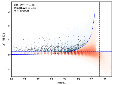
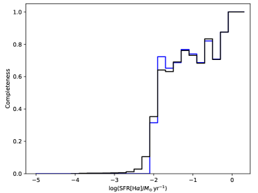
Figure 12: NB selection diagram (left panel) and completeness limit for SFR (right panel) for NB921 excess emitters using the best fit model, $\left<\log{\rm EW}\right>=1.45$ and $\sigma[\log({\rm EW})]=0.45$. Blue dashed lines indicate our NB excess selection with the vertical dashed line indicating the NB921 3$\sigma$ limit. Blue (red) points indicate galaxies that meet (miss) our selection, with color intensity indicating more galaxies. The right panel illustrates that our selection reaches a plateau at high SFRs due to missing low-sSFR galaxies. It then follows a monotonic decrease with lower SFRs. The black (blue) line is based on modeled (measured) SFRs.

Table 5: Summary of NB Selections

Filter	(NB–BB)min	EWobs,min	EWrest,min	$\log{F_{\rm NB}}$	$\left<\log({\rm EW})\right>$	$\sigma[\log({\rm EW})]$	$C$(sSFR)	$C$(SFR[H$\alpha$])
(1)	(2)	(3)	(4)	(5)	(6)	(7)	(8)	(9)
NB704	0.15	16.5	15.4	-17.26	1.25	0.55	-10.22	-3.66
NB711	0.15	11.5	10.6	-17.20	1.05	0.75	-10.20	-3.45
NB816	0.15	19.7	15.9	-17.36	1.25	0.45	-10.19	-2.57
NB921	0.20	32.0	22.8	-17.23	1.45	0.45	-10.06	-1.78
NB973	0.25	70.3	47.3	-16.77	1.25	0.45	-9.69	-0.09

• (1) NB filter. (2) Minimum NB color excess in magnitudes. (3) Minimum observed H$\alpha$+[N ii] EW in Angstroms. (4) Minimum rest-frame H$\alpha$+[N ii] EW in Angstroms. (5) Logarithm of 3-$\sigma$ NB excess flux limit in erg s^-1 cm^-2. (6)–(7) Best log-normal EW distribution model described with mean and dispersion. (8)–(9) Completeness limit at 50% for $\log\left({\rm sSFR/yr}^{-1}\right)$ and $\log\left(\frac{{\rm SFR[H}\alpha]}{M_{\odot}~{}{\rm yr}^{-1}}\right)$.

6 Conclusions

With our sample of 714 H$\alpha$ emitting NB-selected galaxies from the Metal Abundances across Cosmic Time ($\mathcal{MACT}$) Survey, we have been able to observationally extend the “star formation main sequence" and the specific SFR evolution down to 10${}^{6}M_{\odot}$, a domain that had not yet been explored with observed individual galaxies outside of the local Universe ($z\gtrsim 0.07$). Our key results are as follows:

1. Our H$\alpha$-derived SFRs are systematically underpredicted relative to FUV-derived SFRs, in agreement with observations of local galaxies (e.g., Lee et al., 2009).

2. At a given stellar mass, $\log(M_{\star}/M_{\odot})=8.0\pm 0.5$, there is significant evolution for the specific SFR: ${\log\left(\rm sSFR\right)\propto A\log(1+z)}$ with $A=5.26\pm 0.75$. On average, low-mass galaxies have higher sSFR than more massive ($3\times 10^{9}M_{\odot}$) galaxies, with the sSFR nearly reaching a plateau at low stellar masses.

3. The SFR–$M_{\star}$ relation holds for galaxies spanning $\sim$10⁶–$10^{10}~{}M_{\odot}$ at $z\approx$ 0.07–0.5, and follows a redshift-dependent relation of $\log{({\rm SFR})}\propto\alpha\log(M_{\star}/M_{\odot})+\beta z$ with $\alpha=0.60\pm 0.01$ and $\beta=1.86\pm 0.07$. Our results do not significantly differ from recent studies that have also explored the SFR–$M_{\star}$ relation for low-mass galaxies, albeit across slightly different redshift ranges (e.g., McGaugh et al., 2017; Boogaard et al., 2018).

4. The observed intrinsic dispersion of our galaxies appears to be fairly well regulated ($\approx$0.3 dex), in agreement with other observational work at comparable redshifts. With corrections for survey selection effects that miss low specific SFR galaxies, we find that our observed intrinsic dispersion may be underestimated by a factor of $\approx$2 such that the true dispersion is $\approx$0.5 dex. We do not observe any evidence for increasing or decreasing scatter over our mass range, 10⁶–10${}^{10}~{}M_{\odot}$, which is consistent with results obtained at similar or higher masses.

Data availability

The data in this article are available upon request to the corresponding author.

Appendix A Color selection plots

In this appendix, we illustrate the broad-band color selections that were adopted to identify H$\alpha$ emitters. We refer to Section 3.1 for more details on the color selections and the H$\alpha$ samples.

Appendix B Summary of composite spectra measurements

In this appendix, we provide figures that illustrate our composite spectra, as well as tables that summarise our results. We refer to Section 3.2 for more details on the composite spectral stacking and emission-line fitting.

Table 6: Summary of measurements from MMT/Hectospec composite spectra

$\log(M_{\star}/M_{\odot})$	$N_{\rm H\gamma}$	$N_{\rm H\beta}$	$N_{\rm H\alpha}$	$F_{\rm H\beta}$	$F_{\rm H\gamma}$/$F_{\rm H\beta}$	$F_{\rm H\alpha}$/$F_{\rm H\beta}$	$E$($B$–$V$)Hγ	$E$($B$–$V$)Hα	$F_{[\textsc{N~{}ii}]}$/$F_{\rm H\alpha}$
(1)	(2)	(3)	(4)	(5)	(6)	(7)	(8)	(9)	(10)
NB704+NB711 ($z=0.068$–0.091)
6.17–7.20	12	12	12	34.84${}_{-0.54}^{+0.57}$	0.50${}_{-0.01}^{+0.01}$	2.15${}_{-0.01}^{+0.01}$	0.000${}_{-0.035}^{+0.037}$	0.000${}_{-0.006}^{+0.007}$	0.14
7.28–8.55	12	12	12	55.25${}_{-1.18}^{+1.25}$	0.28${}_{-0.02}^{+0.01}$	2.40${}_{-0.04}^{+0.04}$	0.988${}_{-0.098}^{+0.107}$	0.000${}_{-0.016}^{+0.016}$	0.04
NB816 ($z=0.229$–0.252)
7.23–7.60	10	10	10	16.15${}_{-0.67}^{+0.70}$	0.40${}_{-0.03}^{+0.03}$	2.25${}_{-0.04}^{+0.04}$	0.285${}_{-0.133}^{+0.157}$	0.000${}_{-0.017}^{+0.019}$	0.08
7.70–7.93	10	10	10	35.61${}_{-0.66}^{+0.70}$	0.44${}_{-0.01}^{+0.01}$	2.04${}_{-0.01}^{+0.01}$	0.133${}_{-0.037}^{+0.039}$	0.000${}_{-0.006}^{+0.006}$	0.08
7.97–8.17	10	10	10	23.00${}_{-0.55}^{+0.53}$	0.31${}_{-0.02}^{+0.02}$	2.10${}_{-0.01}^{+0.01}$	0.815${}_{-0.107}^{+0.122}$	0.000${}_{-0.004}^{+0.005}$	0.01
8.21–8.60	9	9	9	77.13${}_{-0.66}^{+0.60}$	0.37${}_{-0.00}^{+0.00}$	2.16${}_{-0.01}^{+0.01}$	0.470${}_{-0.024}^{+0.024}$	0.000${}_{-0.004}^{+0.004}$	0.10
8.65–9.49	10	10	10	60.97${}_{-1.03}^{+0.87}$	0.34${}_{-0.01}^{+0.01}$	2.54${}_{-0.02}^{+0.02}$	0.618${}_{-0.056}^{+0.055}$	0.000${}_{-0.007}^{+0.007}$	0.54
NB921 ($z=0.389$–0.413)
6.64–7.93	36	36	1	6.13${}_{-0.28}^{+0.30}$	0.48${}_{-0.03}^{+0.03}$	…	0.000${}_{-0.111}^{+0.131}$	…	…
7.96–8.24	34	34	…	9.16${}_{-0.31}^{+0.33}$	0.46${}_{-0.01}^{+0.01}$	…	0.022${}_{-0.046}^{+0.051}$	…	…
8.25–8.46	35	35	7	17.69${}_{-0.26}^{+0.25}$	0.45${}_{-0.01}^{+0.01}$	1.69${}_{-0.05}^{+0.05}$	0.062${}_{-0.049}^{+0.052}$	0.000${}_{-0.031}^{+0.030}$	0.05
8.47–8.79	36	36	8	19.17${}_{-0.39}^{+0.35}$	0.57${}_{-0.00}^{+0.00}$	2.26${}_{-0.08}^{+0.08}$	0.000${}_{-0.016}^{+0.016}$	0.000${}_{-0.035}^{+0.033}$	0.02
8.81–10.27	36	36	10	40.49${}_{-0.55}^{+0.46}$	0.41${}_{-0.00}^{+0.00}$	1.50${}_{-0.05}^{+0.04}$	0.260${}_{-0.021}^{+0.020}$	0.000${}_{-0.031}^{+0.029}$	0.17
NB973 ($z=0.453$–0.499)
7.24–8.24	13	13	…	17.88${}_{-0.61}^{+0.65}$	0.45${}_{-0.01}^{+0.01}$	…	0.072${}_{-0.040}^{+0.044}$	…	…
8.27–8.74	13	13	…	48.96${}_{-0.96}^{+1.02}$	0.45${}_{-0.00}^{+0.00}$	…	0.092${}_{-0.015}^{+0.015}$	…	…
8.76–8.94	13	13	…	27.12${}_{-0.95}^{+0.91}$	0.58${}_{-0.00}^{+0.00}$	…	0.000${}_{-0.000}^{+0.000}$	…	…
8.98–9.33	13	13	…	34.90${}_{-0.72}^{+0.65}$	0.52${}_{-0.00}^{+0.00}$	…	0.000${}_{-0.015}^{+0.015}$	…	…
9.53–10.43	13	13	…	33.05${}_{-1.00}^{+0.84}$	0.38${}_{-0.01}^{+0.01}$	…	0.406${}_{-0.074}^{+0.076}$	…	…

• (1): Stellar mass range. (2)–(4): Number of galaxies in composite spectra for H$\gamma$, H$\beta$, and H$\alpha$. (5): Emission-line fluxes in units of 10^-18 erg s^-1 cm^-2 for H$\beta$. (6)–(7): H$\gamma$/H$\beta$ and H$\alpha$/H$\beta$ Balmer decrement. (8)–(9): $E$($B$–$V$) derived from H$\gamma$/H$\beta$ and H$\alpha$/H$\beta$ flux ratios. (10): [N ii]$\lambda\lambda$6548,6583/H$\alpha$ flux ratio.

Table 7: Summary of measurements from Keck-II/DEIMOS composite spectra

$\log(M_{\star}/M_{\odot})$	$N_{\rm H\beta}$	$N_{\rm H\alpha}$	$F_{\rm H\beta}$	$F_{\rm H\alpha}$/$F_{\rm H\beta}$	$E$($B$–$V$)Hα	$F_{[\textsc{N~{}ii}]}$/$F_{\rm H\alpha}$
(1)	(2)	(3)	(4)	(5)	(6)	(7)
NB921 ($z=0.389$–0.428)
6.39–7.96	19	19	3.61${}_{-0.14}^{+0.15}$	3.22${}_{-0.10}^{+0.10}$	0.120${}_{-0.032}^{+0.032}$	0.02
7.97–8.24	18	17	6.92${}_{-0.18}^{+0.17}$	2.77${}_{-0.05}^{+0.05}$	0.000${}_{-0.018}^{+0.018}$	0.03
8.28–8.51	17	17	17.61${}_{-0.19}^{+0.19}$	3.04${}_{-0.02}^{+0.03}$	0.062${}_{-0.007}^{+0.008}$	0.08
8.53–8.99	18	18	28.74${}_{-0.24}^{+0.23}$	2.87${}_{-0.02}^{+0.02}$	0.005${}_{-0.007}^{+0.007}$	0.12
9.00–9.72	19	19	52.18${}_{-0.49}^{+0.50}$	3.01${}_{-0.02}^{+0.02}$	0.051${}_{-0.008}^{+0.008}$	0.29
NB973 ($z=0.458$–0.498)
7.24–8.31	11	10	14.56${}_{-0.25}^{+0.26}$	2.61${}_{-0.01}^{+0.01}$	0.000${}_{-0.005}^{+0.005}$	0.00
8.35–8.73	10	8	54.21${}_{-0.23}^{+0.22}$	2.90${}_{-0.00}^{+0.00}$	0.015${}_{-0.001}^{+0.001}$	0.02
8.76–9.05	11	9	40.69${}_{-0.27}^{+0.26}$	3.15${}_{-0.00}^{+0.00}$	0.096${}_{-0.001}^{+0.001}$	0.03
9.13–9.43	9	6	28.34${}_{-0.38}^{+0.36}$	2.98${}_{-0.04}^{+0.04}$	0.040${}_{-0.014}^{+0.014}$	0.11
9.54–10.27	11	7	33.62${}_{-0.44}^{+0.45}$	2.87${}_{-0.00}^{+0.00}$	0.003${}_{-0.001}^{+0.001}$	0.54

• (1): Stellar mass range. (2)–(3): Number of galaxies in composite spectra for H$\beta$ and H$\alpha$. (4): Emission-line fluxes in units of 10^-18 erg s^-1 cm^-2 for H$\beta$. (5) H$\alpha$/H$\beta$ Balmer decrement. (6): $E$($B$–$V$) derived from H$\alpha$/H$\beta$ Balmer decrement. (7): [N ii]$\lambda\lambda$6548,6583/H$\alpha$ flux ratio.

Appendix C Summary of SFR–$M_{\star}$ relation

In this appendix, we summarise in the following table the results of our SFR-$M_{\star}$ relation as function of redshift. We refer to Section 5.3 for the analyses.

Table 8: Summary of redshift-dependent SFR–$M_{\star}$ relation.

$\log\left(\frac{M_{\star}}{M_{\odot}}\right)$	NB704, NB711				NB816				NB921				NB973
	$N$	$\left<M\right>$	$\left<{\rm SFR}\right>$		$N$	$\left<M\right>$	$\left<{\rm SFR}\right>$		$N$	$\left<M\right>$	$\left<{\rm SFR}\right>$		$N$	$\left<M\right>$	$\left<{\rm SFR}\right>$
(1)	(2)	(3)	(4)		(5)	(6)	(7)		(8)	(9)	(10)		(11)	(12)	(13)
6.0–6.5	16	6.30	–2.56 (–3.10)		2	6.27	–2.06 (–2.41)		…	…	…		…	…	…
6.5–7.0	16	6.73	–2.47 (–2.98)		12	6.78	–1.99 (–2.31)		1	6.64	–1.20 (–1.37)		…	…	…
7.0–7.5	16	7.19	–2.21 (–2.63)		31	7.32	–1.87 (–2.15)		18	7.32	–1.31 (–1.48)		3	7.24	–0.52 (–0.68)
7.5–8.0	10	7.75	–1.79 (–2.05)		41	7.74	–1.54 (–1.77)		63	7.80	–1.31 (–1.48)		13	7.76	–0.57 (–0.74)
8.0–8.5	1	8.40	–1.73 (–1.95)		41	8.22	–1.32 (–1.51)		102	8.25	–1.11 (–1.28)		26	8.26	–0.69 (–0.85)
8.5–9.0	1	8.55	–1.53 (–1.69)		18	8.72	–0.84 (–1.00)		79	8.73	–0.79 (–0.95)		66	8.75	–0.50 (–0.67)
9.0–9.5	…	…	…		8	9.26	–0.36 (–0.52)		45	9.23	–0.25 (–0.41)		35	9.16	–0.18 (–0.35)
9.5–10.0	…	…	…		1	9.52	–0.40 (–0.57)		18	9.77	+0.12 (–0.05)		23	9.66	+0.14 (–0.03)
10.0–10.5	…	…	…		…	…	…		2	10.25	+0.13 (–0.04)		6	10.22	+0.41 (+0.24)

• (1): Stellar mass range. (2)–(13): Number of galaxies, average log stellar mass, and average log SFR (average log SFR without FUV corrections) for NB704 and/or NB711 emitters (2)–(4), NB816 emitters (5)–(7), NB921 emitters (8)–(10), and NB973 emitters (11)–(13). Bins with five or fewer galaxies have less reliable derived SFR measurements, possibly due to selection effects of NB emission-line flux limits at the faint end and minimum EW excess at the bright end.

References

- Astropy Collaboration et al. (2013) Astropy Collaboration, Robitaille, T. P., Tollerud, E. J., et al. 2013, A&A, 558, A33
- Astropy Collaboration et al. (2018) Astropy Collaboration, Price-Whelan, A. M., Sipõcz, B. M., et al. 2018, AJ, 156, 123
- Atek et al. (2014) Atek, H., Kneib, J.-P., Pacifici, C., et al. 2014, ApJ, 789, 96
- Bacon et al. (2010) Bacon, R., Accardo, M., Adjali, L., et al. 2010, Proc. SPIE, 773508
- Berg et al. (2012) Berg, D. A., et al., 2012, ApJ, 754, 98
- Bertin & Arnouts (1996) Bertin, E., & Arnouts, S. 1996, A&AS, 117, 393
- Boogaard et al. (2018) Boogaard, L. A., Brinchmann, J., Bouché, N., et al. 2018, A&A, 619, A27
- Brammer et al. (2008) Brammer, G. B., van Dokkum, P. G., & Coppi, P. 2008, ApJ, 686, 1503-1513
- Bressan et al. (1993) Bressan, A., Fagotto, F., Bertelli, G., et al. 1993, A&AS, 100, 647
- Brinchmann et al. (2004) Brinchmann, J., Charlot, S., White, S. D. M., et al. 2004, MNRAS, 351, 1151
- Bruzual & Charlot (2003) Bruzual, G., & Charlot, S. 2003, MNRAS, 344, 1000
- Calzetti et al. (2000) Calzetti, D., Armus, L., Bohlin, R. C., et al. 2000, ApJ, 533, 682
- Cardelli et al. (1989) Cardelli, J. A., Clayton, G. C., & Mathis, J. S. 1989, ApJ, 345, 245
- Chabrier (2003) Chabrier, G. 2003, PASP, 115, 763
- Cooper et al. (2012) Cooper, M. C., Newman, J. A., Davis, M., Finkbeiner, D. P., & Gerke, B. F. 2012, Astrophysics Source Code Library, ascl:1203.003
- Daddi et al. (2007) Daddi, E., Dickinson, M., Morrison, G., et al. 2007, ApJ, 670, 156
- Dave et al. (2012) Dave, R., Finlator, K., & Oppenheimer, B. D. 2012, MNRAS, 421, 98
- Davies et al. (2019) Davies L. J. M., Lagos C. del P., Katsianis A., Robotham A. S. G., Cortese L., Driver S. P., Bremer M. N., et al., 2019, MNRAS, 483, 1881
- de los Reyes et al. (2015) de los Reyes, M. A., Ly, C., Lee, J. C., et al. 2015, AJ, 149, 79
- Domínguez et al. (2015) Domínguez, A., Siana, B., Brooks, A. M., et al. 2015, MNRAS, 451, 839
- Dutton et al. (2010) Dutton, A. A., van den Bosch, F. C., & Dekel, A. 2010, MNRAS, 405, 1690
- Emami et al. (2019) Emami, N., Siana, B., Weisz, D. R., et al. 2019, ApJ, 881, 71
- Erb et al. (2006) Erb, D. K., Shapley, A. E., Pettini, M., et al. 2006, ApJ, 644, 813
- Faber et al. (2003) Faber, S. M., Phillips, A. C., Kibrick, R. I., et al. 2003, Proc. SPIE, 4841, 1657
- Fabricant et al. (2005) Fabricant, D., Fata, R., Roll, J., et al. 2005, PASP, 117, 1411
- Fagotto et al. (1994) Fagotto, F., Bressan, A., Bertelli, G., et al. 1994, A&AS, 105, 29
- Fujita et al. (2003) Fujita, S. S., Ajiki, M., Shioya, Y., et al. 2003, ApJ, 586, L115
- Garn & Best (2010) Garn T., Best P. N., 2010, MNRAS, 409, 421
- Gonzalez et al. (2011) Gonzalez, V., Labbe, I., Bouwens, R. J., et al. 2011, ApJ, 735, L34
- Harris et al. (2020) Harris, C. R., Millman, K. J., van der Walt, S. J., et al. 2020, Nature, 585, 357
- Hunter (2007) Hunter, J. D. 2007, Computing in science & engineering, 9, 90
- Iyer et al. (2018) Iyer, K., et al., 2018, ApJ, 866, 120
- Jones et al. (2001) Jones, E., Oliphant, T., Peterson, P., et al. 2001, http://www.scipy.org/
- Karim et al. (2011) Karim, A., Schinnerer, E., Martínez-Sansigre, A., et al. 2011, ApJ, 730, 61
- Kashikawa et al. (2004) Kashikawa, N., Shimasaku, K., Yasuda, N., et al. 2004, PASJ, 56, 1011
- Kashikawa et al. (2006) Kashikawa, N., Yoshida, M., Shimasaku, K., et al. 2006, ApJ, 637, 631
- Kashikawa et al. (2011) Kashikawa, N., Shimasaku, K., Matsuda, Y., et al. 2011, ApJ, 734, 119
- Kennicutt (1998) Kennicutt, R. C., Jr. 1998, ARA&A, 36, 189
- Kennicutt et al. (2008) Kennicutt, R. C., Jr., Lee, J. C., Funes, J. G., et al. 2008, ApJS, 178, 247
- Kennicutt & Evans (2012) Kennicutt R. C., Evans N. J., 2012, ARA&A, 50, 531
- Kriek et al. (2009) Kriek, M., van Dokkum, P. G., Labbé, I., et al. 2009, ApJ, 700, 221
- Kroupa (2001) Kroupa, P. 2001, MNRAS, 322, 231
- Kroupa & Weidner (2003) Kroupa P., Weidner C., 2003, ApJ, 598, 1076
- Lee et al. (2009) Lee, J. C., et al. 2009, ApJ, 706, 599
- Lee et al. (2012) Lee, J. C., et al. 2012, PASP, 124, 782
- Lee et al. (2015) Lee, N. C., et al. 2015, ApJ, 801, 80
- Lee et al. (2007) Lee, J. C., Kennicutt, R. C., Funes, S. J., José G., Sakai, S., & Akiyama, S. 2007, ApJ, 671, L113
- Lehnert et al. (2015) Lehnert, M. D., van Driel, W., Le Tiran, L., et al. 2015, A&A, 577, A112
- Leitherer et al. (1999) Leitherer, C., Schaerer, D., Goldader, J. D., et al. 1999, ApJS, 123, 3
- Ly et al. (2007) Ly, C., Malkan, M. A., Kashikawa, N., et al. 2007, ApJ, 657, 738
- Ly et al. (2009) Ly, C., Malkan, M. A., Treu, T., et al. 2009, ApJ, 697, 1410
- Ly et al. (2011a) Ly, C., Malkan, M. A., Hayashi, M., et al. 2011a, ApJ, 735, 91
- Ly et al. (2011b) Ly, C., Lee, J. C., Dale, D. A., et al. 2011b, ApJ, 726, 109
- Ly et al. (2012a) Ly, C., Malkan, M. A., Kashikawa, N., et al. 2012, ApJ, 747, L16
- Ly et al. (2012b) Ly, C., Malkan, M. A., Kashikawa, N., et al. 2012, ApJ, 757, 63
- Ly et al. (2016) Ly, C., Malhotra, S., Malkan, M. A., et al. 2016, ApJS, 226, 5
- McGaugh et al. (2017) McGaugh, S. S., Schombert, J. M., & Lelli, F. 2017, ApJ, 851, 22
- Madau & Dickinson (2014) Madau, P., & Dickinson, M. 2014, ARA&A, 52, 415
- Martin et al. (2005) Martin, D. C., Fanson, J., Schiminovich, D., et al. 2005, ApJ, 619, L1
- Miyazaki et al. (2002) Miyazaki, S., Komiyama, Y., Sekiguchi, M., et al. 2002, PASJ, 54, 833
- Nagao et al. (2008) Nagao, T., Sasaki, S. S., Maiolino, R., et al. 2008, ApJ, 680, 100-109
- Noeske et al. (2007) Noeske, K. G., Weiner, B. J., Faber, S. M., et al. 2007, ApJ, 660, L43
- Oliphant (2006) Oliphant, T. E. 2006, A guide to NumPy, Vol. 1 (Trelgol Publishing USA)
- Osterbrock & Ferland (2006) Osterbrock D. E., Ferland G. J., 2006, Astrophysics of gaseous nebulae and active galactic nuclei, 2nd. ed. University Science Books, Sausalito California
- Pettini & Pagel (2004) Pettini, M., & Pagel, B. E. J. 2004, MNRAS, 348, L59
- Renzini (2009) Renzini, A. 2009, MNRAS, 398, L58
- Rodighiero et al. (2011) Rodighiero, G., Daddi, E., Baronchelli, I., et al. 2011, ApJ, 739, L40
- Salim et al. (2007) Salim, S., Rich, R. M., Charlot, S., et al. 2007, ApJS, 173, 267
- Salpeter (1955) Salpeter, E. E. 1955, ApJ, 121, 161
- Schreiber et al. (2015) Schreiber C., Pannella M., Elbaz D., Béthermin M., Inami H., Dickinson M., Magnelli B., et al., 2015, å, 575, A74
- Speagle et al. (2014) Speagle J. S., Steinhardt C. L., Capak P. L., Silverman J. D., 2014, ApJS, 214, 15
- Stetson (1987) Stetson, P. B. 1987, PASP, 99, 191
- Tasca et al. (2015) Tasca, L. A. M., Le Fèvre, O., Hathi, N. P., et al. 2015, A&A, 581, A54
- Virtanen et al. (2020) Virtanen P., Gommers R., Oliphant T. E., Haberland M., Reddy T., Cournapeau D., Burovski E., et al., 2020, NatMe, 17, 261
- Weidner et al. (2013) Weidner C., Kroupa P., Pflamm-Altenburg J., Vazdekis A., 2013, MNRAS, 436, 3309
- Whitaker et al. (2012b) Whitaker, K. E., van Dokkum, P. G., Brammer, G., & Franx, M. 2012, ApJ, 754, L29
- Whitaker et al. (2014) Whitaker, K. E., Franx, M., Leja, J., et al. 2014, ApJ, 795, 104