KEK-TH-2160

F-theory Flux Vacua and Attractor Equations
Yoshinori Honma^a and Hajime Otsuka^b
aDepartment of Current Legal Studies,
Meiji Gakuin University,
Yokohama, Kanagawa 244-8539, Japan
^bTheory Center, Institute of Particle and Nuclear Studies,
High Energy Accelerator Research Organization, KEK,
1-1 Oho, Tsukuba, Ibaraki 305-0801, Japan

We examine the vacuum structure of 4D effective theories of moduli fields in spacetime compactifications with quantized background fluxes. Imposing the no-scale structure for the volume deformations, we numerically investigate the distributions of flux vacua of the effective potential in complex structure moduli and axio-dilaton directions for two explicit examples in Type IIB string theory and F-theory compactifications. It turns out that distributions of non-supersymmetric flux vacua exhibit a non-increasing functional behavior of several on-shell quantities with respect to the string coupling. We point out that this phenomena can be deeply connected with a previously-reported possible correspondence between the flux vacua in moduli stabilization problem and the attractor mechanism in supergravity, and our explicit demonstration implies that such a correspondence generically exist even in the framework of F-theory. In particular, we confirm that the solutions of the effective potential we explicitly evaluated in Type IIB and F-theory flux compactifications indeed satisfy the generalized form of the attractor equations simultaneously.

1 Introduction

Stabilization of extra massless scalar moduli fields of 4D effective theories arising from spacetime compactifications is of particular interest in the field of string theory and its broad applications to cosmology and phenomenology. In particular, remarkable progress for cosmological observations in recent years has motivated us to realize de Sitter spacetime with stabilized moduli in the framework of string theory and contrive a concrete setup in which basic quantum gravitational issues can be thoroughly investigated. In the study of this moduli stabilization problem, one looks at the scalar potential of 4D ${\cal{N}}=1$ effective theories arising from spacetime compactifications. In the language of 4D ${\cal{N}}=1$ supersymmetry, there are two kinds of contributions to the scalar potential of moduli fields, namely the K$\ddot{{\textrm{a}}}$hler potential and the superpotential. String compactifications enables us to derive these quantities quantum mechanically from the geometry of internal compact spaces, often taken to be a Calabi-Yau manifold to use sufficient amount of supersymmetry while keeping the problem nontrivial. Inclusion of background fluxes is a crucial ingredient to generate interactions between moduli fields in superpotential, leading to their stabilization in a controllable way.

To grasp the background and clarify our motivation for the present paper in more detail, let us begin with the 4D effective action arising from Type IIB Calabi-Yau orientifolds or the F-theory on Calabi-Yau fourfolds [1], both of which can be described by the 4D ${\cal{N}}=1$ supergravity language. Suppose the K$\ddot{{\textrm{a}}}$hler moduli fields labeled by $\alpha$ are absent in the superpotential $W$, and also the K$\ddot{{\textrm{a}}}$hler potential $K$ satisfies the condition $K^{\alpha\bar{\alpha}}\partial_{\alpha}K\partial_{\bar{\alpha}}\overline{K}=3$, the $F$-term scalar potential of moduli fields becomes a no-scale type

$$V=e^{K}\left(K^{I\bar{J}}D_{I}WD_{\bar{J}}\overline{W}\right),$$ (1.1)

in the reduced Planck mass unit $M_{\rm Pl}=1$. Here $I,J$ run over the complex structure moduli of a Calabi-Yau threefold and the axio-dilaton in a Type IIB setup, which can be also regarded as a unified complex structure moduli of a Calabi-Yau fourfold from the F-theory perspective. Here $D_{I}\equiv\partial_{I}+(\partial_{I}K)$ denote the K$\ddot{{\textrm{a}}}$hler covariant derivative and $K^{I\bar{J}}$ is the inverse of the K$\ddot{{\textrm{a}}}$hler metric $K_{I\bar{J}}=\partial_{I}\partial_{\bar{J}}K$. Throughout this paper, we focus on this no-scale type potential.

It is well known that the imaginary self-dual three-form fluxes in Type IIB string theory or the self-dual four-form fluxes in F-theory can generate suitable flux superpotential $W$ to stabilize moduli fields at $D_{I}W=0$, leading to stable Minkowski minima [2, 3, 4]. While this prescription completely fix the complex structure moduli and axio-dilaton, the K$\ddot{{\textrm{a}}}$hler moduli of the compactification remain unfixed. In order to fix all the moduli and construct realistic cosmologies describing the accelerated expansion of the universe, quantum $\alpha^{\prime}$-corrections and non-perturbative effects should be further included. This issue has been resolved in the explicit constructions of the Kachru-Kallosh-Linde-Trivedi (KKLT) model [5] and the LARGE Volume Scenario (LVS) [6, 7]. There the small value of de Sitter cosmological constant for the late-time cosmology has been realized by an inclusion of the anti-D3-brane inducing an uplifting potential.

On the other hand, as has been pointed out for instance in [8], effective theories equipped with the no-scale type potential can also accommodate supersymmetry-breaking minima with $V\neq 0$ in complex structure moduli and axio-dilaton directions. There the spontaneous supersymmetry breaking effect due to a small vacuum energy can be regarded as a variant of the anti-D-branes to produce tiny cosmological constant. In the same spirit, several supersymmetry-breaking scenarios has been discussed, for instance, in [9, 10]. While such an uplifting mechanism may have broad applications to de Sitter model building, comprehensive study has not been fully elucidated, possibly due to the complexity of analysis of the non-supersymmetric vacua. One of our goals in the present paper is to fill this gap and understand the characteristics of the flux vacua in general compactifications.

Specifically, we investigate the vacuum structure of two explicit examples in Type IIB string theory and F-theory compactifications while assuming the no-scale structure (1.1). By solving the system numerically and finding the non-supersymmetric flux vacua in both setups, we find that several on-shell quantities exhibit a non-increasing functional behavior with respect to the string coupling. In the process of clarifying an underlying dynamics of this phenomena, we find that this characteristic behavior of flux vacua can be regarded as a direct consequence of a previously-studied possible correspondence between moduli stabilization problem and attractor mechanism in supergravity emphasized in [11] (see also [12, 13, 14, 15, 16]), and our demonstration provides a nontrivial supporting evidence for this kind of correspondence. Especially, one can check that our numerical solutions as well as analytic Minkowski solutions indeed satisfy the appropriately generalized attractor equation simultaneously, even in the framework of F-theory.

This paper is organized as follows. We first take a brief look at an effective theory arising from Type IIB toroidal orientifold compactification and study its vacuum structure in Section 2. In Section 3, we move on to analyze the effective potential of moduli fields arising from F-theory compactified on a Calabi-Yau fourfold. Finally in Section 4, we reconsider our results from another viewpoint and confirm that the moduli stabilization problem discussed in Sections 2 and 3 can be rephrased in terms of the attractor mechanism in supergravity. Section 5 is devoted to conclusions and discussions. In Appendix A, we describes the F-theory generalization of the attractor equation.

2 Type IIB Toroidal Orientifold

First we consider a well-known Type IIB toroidal orientifold model and investigate its vacuum structure. Explicit demonstrations in this simple setup would make the arguments in subsequent sections more intelligible.

2.1 Setup

Here we briefly look at the effective potential of moduli fields in Type IIB string theory compactified on a $T^{6}/\mathbb{Z}_{2}$ toroidal orientifold. We refer the reader to [17, 18] for the details about the construction.

Let us represent the periodic six real coordinates on $T^{6}$ by $x^{i}$ and $y^{i}$ with $i,j=1,2,3$, and take the holomorphic one-forms of the $T^{2}$ submanifolds as $dz^{i}=dx^{i}+\tau^{ij}dy^{j}$. By choosing the orientation as $\int_{T^{6}}dx^{1}\wedge dx^{2}\wedge dx^{3}\wedge dy^{1}\wedge dy^{2}\wedge dy^{3}=1$ and representing the three-form cohomology basis in $H^{3}(T^{6},\mathbb{Z})$ as

$$\begin{split}\alpha_{0}&=dx^{1}\wedge dx^{2}\wedge dx^{3},\ \ \ \ \ \ \ \ \ \ \ \alpha_{ij}=\frac{1}{2}\epsilon_{ikl}dx^{k}\wedge dx^{l}\wedge dy^{j},\\ \beta^{ij}&=-\frac{1}{2}\epsilon_{jkl}dy^{k}\wedge dy^{l}\wedge dx^{i},\ \ \ \ \beta_{0}=dy^{1}\wedge dy^{2}\wedge dy^{3},\end{split}$$ (2.1)

the holomorphic three-form $\Omega\equiv dz^{1}\wedge dz^{2}\wedge dz^{3}$ on $T^{6}/\mathbb{Z}_{2}$ can be described as

$$\Omega=\alpha_{0}+\alpha_{ij}\tau^{ij}-\frac{1}{2}\beta^{ij}(\epsilon_{ikl}\epsilon_{jmn}\tau^{km}\tau^{ln})+\beta^{0}({\rm det}\tau).$$ (2.2)

Here the matrices $\tau^{ij}$ describe the complex structure moduli of the geometry and the three-form cohomology basis is normalized as $\int_{T^{6}}\alpha_{I}\wedge\beta^{J}=\delta_{I}^{J}$. The three-form fluxes $F_{3}$ and $H_{3}$ in RR and NSNS sectors in Type IIB string theory can be expanded in the same basis as

$$\begin{split}&\frac{1}{(2\pi)^{2}\alpha^{\prime}}F_{3}=a^{0}\alpha_{0}+a^{ij}\alpha_{ij}+b_{ij}\beta^{ij}+b_{0}\beta^{0},\\ &\frac{1}{(2\pi)^{2}\alpha^{\prime}}H_{3}=c^{0}\alpha_{0}+c^{ij}\alpha_{ij}+d_{ij}\beta^{ij}+d_{0}\beta^{0},\end{split}$$ (2.3)

where the coefficients $a^{0},a^{ij},b_{0},b_{ij},c^{0},c^{ij},d_{0},d_{ij}\in 2\mathbb{Z}$ describe the quanta of background fluxes. Note that here we focus on even numbers of flux quanta to prohibit the appearance of delicate exotic O3-planes [18].

The explicit form of the K$\ddot{{\textrm{a}}}$hler potential for moduli fields is given by

$$K=-\ln{\left[-i(S-\overline{S})\right]}-\ln{\left[-i\int\Omega\wedge\bar{\Omega}\right]}-2\ln{\cal{V}},$$ (2.4)

where $S$ denotes the axio-dilaton. The hermitian norm of $\Omega$ corresponds to the Weil-Petersson metric of the complex structure moduli space and ${\cal V}$ is a volume of the internal manifold $T^{6}/\mathbb{Z}_{2}$ in the Einstein-frame, measured in units of $2\pi\sqrt{\alpha^{\prime}}$. Plugging (2.4) into the scalar potential (1.1), one finds that $V$ no longer depends on the K$\ddot{{\textrm{a}}}$hler moduli fields except for a prefactor $\frac{1}{{\cal V}^{2}}>0$ treated as a constant throughout this paper. On the other hand, the superpotential induced by background fluxes in Type IIB compactifications takes the following form [3]

$$W=\frac{1}{\sqrt{4\pi}(2\pi)^{2}\alpha^{\prime}}\int\Omega\wedge G_{3},$$ (2.5)

where $G_{3}\equiv F_{3}-SH_{3}$ denotes the combined three-form fluxes. On $T^{6}/\mathbb{Z}_{2}$ geometry, this becomes

$$\begin{split}W=\frac{1}{\sqrt{4\pi}}\Bigg{(}&(a^{0}-Sc^{0}){\rm det}\tau-\frac{1}{2}(a^{ij}-Sc^{ij})\epsilon_{ikm}\epsilon_{jpq}\tau^{kp}\tau^{mq}\\ &-(b_{ij}-Sd_{ij})\tau^{ij}-(b_{0}-Sd_{0})\Bigg{)}.\end{split}$$ (2.6)

Recalling that there exist $2^{6}$ O3-planes on $T^{6}/{\mathbb{Z}}_{2}$ orientifold, the tadpole cancellation condition

$$32-2n_{{\rm D}3}=\frac{1}{(2\pi)^{4}(\alpha^{\prime})^{2}}\int H_{3}\wedge F_{3}=c^{0}b_{0}+c^{ii}b_{ii}-d_{ii}a^{ii}-d_{0}a^{0},$$ (2.7)

must be also satisfied to ensure the global conservation of fluxes inside the compact manifold. Here $n_{{\rm D}3}$ denotes the number of mobile D3-branes, which is set to be zero in the following discussions.

To simplify the analysis, we further focus on an isotropic case for the system, namely we only consider diagonal components of $\tau^{ij}$ and fluxes satisfying the following condition

$$\begin{split}\tau^{11}&=\tau^{22}=\tau^{33}\equiv\tau,\\ a^{11}&=a^{22}=a^{33}\equiv a^{1},\\ b_{11}&=b_{22}=b_{33}\equiv b_{1},\\ c^{11}&=c^{22}=c^{33}\equiv c^{1},\\ d_{11}&=d_{22}=d_{33}\equiv d_{1},\end{split}$$ (2.8)

as well as the fluxes $\{a^{0},b_{0},c^{0},d_{0}\}$. Then the K$\ddot{{\textrm{a}}}$hler potential (2.4) of the $T^{6}/{\mathbb{Z}}_{2}$ orientifold model reduces to be

$$K=-\ln{\left[(S-\overline{S})(\tau-\overline{\tau})^{3}\right]}-2\ln{\cal{V}},$$ (2.9)

and the flux-induced superpotential becomes

$$W=(4\pi)^{-1/2}\left((a^{0}-Sc^{0})\tau^{3}-3(a^{1}-Sc^{1})\tau^{2}-3(b_{1}-Sd_{1})\tau-(b_{0}-Sd_{0})\right).$$ (2.10)

Combining the above setup with the definition of the no-scale type potential (1.1), one can study the vacuum structure of the model explicitly. Here we consider a condition

$$a^{0}=c^{1}=b_{1}=d_{0}=0,$$ (2.11)

and non-zero otherwise, which corresponds to the imaginary self-dual condition allowing (2,1) and (0,3) piece for $F_{3}$ and the imaginary anti-self-dual condition allowing (3,0) and (1,2) piece for $H_{3}$. This asymmetric choice of background fluxes was chosen to completely fix the complex structure moduli and axio-dilaton, coming from the fact that the $T^{6}/{\mathbb{Z}}_{2}$ toroidal orientifold model originally preserves 4D ${\cal{N}}=4$ supersymmetry. In this setup, the model has a Minkowski minimum as a solution to the $F$-term conditions $D_{I}W=0$, where $V$ becomes zero and the values of moduli fields are fixed as

$${\textrm{Re}}\tau={\textrm{Re}}S=0,\ \ \ \ {\textrm{Im}}\tau=\left(\frac{b_{0}{d_{1}}^{\prime}}{a^{1}c^{0}}\right)^{1/4},\ {\textrm{Im}}S=\left(\frac{(a^{1})^{3}b_{0}}{c^{0}{d_{1}}^{\prime 3}}\right)^{1/4},$$ (2.12)

where ${d_{1}}^{\prime}\equiv-d_{1}$. On the other hand, when we consider a condition

$$c^{0}=a^{1}=d_{1}=b_{0}=0,$$ (2.13)

and non-zero otherwise, this choice corresponds to the imaginary self-dual condition for $H_{3}$ and the imaginary anti-self-dual condition for $F_{3}$. Then the model has a Minkowski minimum at which the values of moduli fields are fixed as

$${\textrm{Re}}\tau ={\textrm{Re}}S=0,\ \ \ \ {\textrm{Im}}\tau=\left(\frac{{b_{1}}^{\prime}{d_{0}}^{\prime}}{a^{0}{c^{1}}^{\prime}}\right)^{1/4},\ {\textrm{Im}}S=\left(\frac{a^{0}({b_{1}}^{\prime})^{3}}{({c^{1}}^{\prime})^{3}{d_{0}}^{\prime}}\right)^{1/4},$$ (2.14)

where ${b_{1}}^{\prime}\equiv-b_{1},{c^{1}}^{\prime}\equiv-c^{1}$ and ${d_{0}}^{\prime}\equiv-d_{0}$. Later we will utilize these simple analytic solutions (2.12) and (2.14) when we discuss about a correspondence between the moduli stabilization and a seemingly different topic in supergravity.

2.2 Distribution of non-supersymmetric flux vacua

Having introduced the setup of the $T^{6}/\mathbb{Z}_{2}$ toroidal orientifold model, now we turn to analyze the non-supersymmetric flux vacua with fixed moduli $\Phi_{I}\equiv\{\tau^{ij},S\}$, while taking into account the tadpole cancellation condition for quantized background fluxes appropriately.

As emphasized in [8], the no-scale type potential (1.1) can also accommodate the supersymmetry-breaking minima characterized by

$$(\partial_{I}V)|_{\Phi_{I}^{0}}=0,\qquad V|_{\Phi_{I}^{0}}=\frac{\epsilon}{{\cal V}^{2}}>0,$$ (2.15)

with the mass squared of the moduli fields being strictly positive. Note that the nonzero vacuum energy at $\Phi_{I}^{0}$ is proportional to a constant Calabi-Yau volume arising from the prefactor $e^{K}$ in the scalar potential, as mentioned in the previous section. Numerical constant $\epsilon$ determined by fluxes can take sufficiently small value owing to the richness of the choice of background fluxes, and this becomes a candidate of the source of an uplifting potential. Throughout this paper, we only pick up the solutions satisfying $\epsilon<1$ as true flux vacua, otherwise the effective theory description of the system turns out to be unreliable.

In our numerical analysis, we utilize the “FindMinimum” function in Mathematica to find supersymmetry-breaking minima of the effective potential. To simplify the analysis, let us again focus on the isotropic case for $\tau^{ij}$ and background fluxes in which the the K$\ddot{{\textrm{a}}}$hler potential and the superpotential are given by (2.9) and (2.10), respectively. Within a flux range $-12\leq a^{0},a^{1},b_{0},b_{1},c^{0},c^{1},d_{0},d_{1}\leq 12$ while imposing the tadpole cancellation condition (2.7) with $n_{\rm D3}=0$, we found 962 supersymmetry-breaking minima with no tachyonic instability.

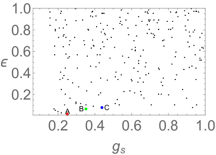
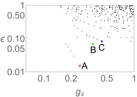
Figure 1: Numerical results for the distribution of flux vacua with nonzero vacuum energy. Each dot corresponds to a solution with different set of fluxes. Note that, however, generically these dots can be degenerated in this 2D plot, due to the existence of another direction of the stabilized moduli $\tau$ which is not depicted here for the simplicity. The right figure represents the log-log plot of the same set of solutions.

The result is depicted in Figure 1, where we plot the height of the normalized potential $\epsilon={\cal V}^{2}V$ with respect to the string coupling $g_{s}\equiv({\rm Im}S)^{-1}$ at the each of the minima. The other on-shell quantities are also shown in Figure 2. Note that generically an ambiguity originating from the Type IIB SL(2,$\mathbb{Z}$) duality transformation generates physically-equivalent solutions and a careful analysis is required. Here and in what follows, we deduct this ambiguity by selecting only the solutions satisfying $|\textrm{Re}S|\leq 1/2$ and $|S|\geq 1$ while keeping the string coupling small but finite: $0<g_{s}<1$.

To provide typical examples of our numerical results, here we pick up three independent flux vacua determined under the following choice of fluxes:

Vacuum	Set of fluxes $(a^{0},a^{1},b_{0},b_{1},c^{0},c^{1},d_{0},d_{1})$
A	$(-2,4,0,-4,0,0,4,-2)$
B	$(4,-4,2,2,0,0,-2,2)$
C	$(-2,2,4,4,0,0,10,-2)$

The vacuum A, B and C are represented in Figure 1 by the red, green and blue points, respectively. Explicit values of stabilized moduli and various on-shell quantities at the each of these flux vacua are summarized in Tables 1 and 2.

Vacuum	$\tau$	$S$	$g_{s}$	$\epsilon$	$W$
A	$0.355+1.64i$	$0.271+3.98i$	0.251	$1.52\times 10^{-2}$	$22.6+5.08i$
B	$0.0468+1.19i$	$0.493+2.84i$	0.352	$6.99\times 10^{-2}$	$-11.6-3.90i$
C	$-0.393+2.48i$	$-0.440+2.29i$	0.438	$8.23\times 10^{-2}$	$14.3+12.6i$

Table 1: Explicit values of stabilized moduli fields and on-shell quantities in $M_{\rm Pl}=1$ unit.

Vacuum	Eigenvalues of mass matrix $\partial_{I}\partial_{J}V\times{\cal V}^{2}$
A	(3.41, 0.603, 0.222, $1.91\times 10^{-2}$)
B	(6.66, 1.30, 0.324, $6.85\times 10^{-2}$)
C	(2.18, 0.690, $7.29\times 10^{-2}$, $9.76\times 10^{-4}$)

Table 2: Mass eigenvalues of normalized scalar potential $\epsilon$ in $M_{\rm Pl}=1$ unit. Note that we have diagonalized the mass matrix ${\cal V}^{2}\partial_{I}\partial_{J}V$ by taking the linear combinations of the basis and the eigenvalues are displayed in the descending order.

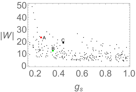
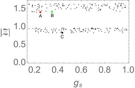
Figure 2: Numerical results for the absolute values of flux superpotential $|W|$ and a quantity $|{\cal Z}|=e^{K/2}|W|$ at the each of the solutions depicted in Figure 1.

From Figures 1 and 2, one finds that the flux vacua of the model seems to be determined such that several on-shell quantities are governed by a nontrivial dynamics, rather than just providing a completely random distribution. Especially, the distribution of a normalized superpotential $|{\cal Z}|=e^{K/2}|W|$ indicates a monotonic, non-increasing functional dependence with respect to the string coupling. As we will see in the next section, another concrete example based on F-theory flux compactification exhibits this kind of dependence of on-shell quantities more clearly. Therefore let us save the arguments for a physical background of this suggestive behavior and its consequences for later discussions in the final section, after looking at the F-theory example and its vacuum structure.

Here we provide some comments on a further consistency check condition to be satisfied, which can be straightforwardly applied to the F-theory compactification described in the next section. To ensure the validity of the effective theory description of the system in the framework of spacetime compactifications, the vacuum energy at the each of the minima needs to be smaller than the mass scales of the Kaluza-Klein and the stringy modes as

$$\langle V\rangle\ll m_{s}^{4},m_{\rm KK}^{4}.$$ (2.16)

In the Type IIB language, these scales are given by $m_{s}=(\alpha^{\prime})^{-1/2}\simeq\frac{g_{s}^{1/4}\sqrt{\pi}}{{\cal V}^{1/2}}$ and $m_{\rm KK}\simeq\frac{\sqrt{\pi}}{{\cal V}^{2/3}}$ in the reduced Planck mass unit. Therefore the above conditions can be rephrased as a requirement that the dimensionless constant $\epsilon$ must satisfy the condition

$$\epsilon\ll{\rm min}({\cal V}^{-2/3}\pi^{2},g_{s}\pi^{2}).$$ (2.17)

For instance if we take a sufficiently large volume ${\cal V}$, e.g. larger than $\simeq{\cal{O}}(10^{2})$, one can estimate that all the numerical solutions summarized in Figure 1 satisfy (2.17). Of course in order to conduct a detailed analysis, ${\cal V}$ needs to be completely fixed by considering an extension of the K$\ddot{{\textrm{a}}}$hler moduli sector beyond our no-scale setup in (2.4).

3 F-theory Model

Let us move on to discuss the 4D ${\cal N}=1$ effective theory based on F-theory flux compactification on a Calabi-Yau fourfold $X_{4}$. After introducing the setup of a model constructed in [25], we numerically analyze the distribution of supersymmetry-breaking minima of its scalar potential in the same manner as performed in the previous section.

3.1 Setup

From the perspective of the F-theory framework, the K$\ddot{{\textrm{a}}}$hler potential for complex structure moduli space of a Calabi-Yau fourfold $X_{4}$ is defined by

$$K=-\ln{\int_{X_{4}}}\Omega\wedge\overline{\Omega},$$ (3.1)

where $\Omega$ denotes a holomorphic $(4,0)$-form on $X_{4}$. The F-theory compactification also generically admits a superpotential of the form [3]

$$W=(4\pi)^{-1/2}\int_{X_{4}}G_{4}\wedge\Omega,$$ (3.2)

in the presence of four-form fluxes $G_{4}$, which is inherited from a duality between F-theory and M-theory on the same manifold [26, 27, 28, 29]. As is the case in the Type IIB orientifold model, background fluxes are required to satisfy the tadpole cancellation condition given by

$$\frac{\chi}{24}=n_{\rm{D3}}+\frac{1}{2}\int_{X_{4}}G_{4}\wedge G_{4},$$ (3.3)

in order to be conserved within a compact manifold $X_{4}$ globally. Here $\chi$ is the Euler characteristic of $X_{4}$ and $n_{\rm{D3}}$ denotes the total number of the mobile D3-branes.

For a Calabi-Yau fourfold $X_{4}$ with $h^{3,1}(X_{4})$ complex structure moduli, the period integrals of holomorphic $(4,0)$-form defined by

$$\Pi_{i}=\int_{\gamma^{i}}\Omega,$$ (3.4)

encode the moduli dependence of the system, and the K$\ddot{{\textrm{a}}}$hler potential for complex structure moduli (3.1) can be rewritten as

$$K=-\ln{\left[\sum_{i,j}\Pi_{i}\eta^{ij}\overline{\Pi}_{j}\right]},$$ (3.5)

where $\gamma^{i}$ with $i=1,\ldots,h^{4}_{H}(X_{4})$ denote a basis of primary horizontal subspace of $H_{4}(X_{4})$. Here we introduced an intersection matrix $\eta^{ij}$ and a dual basis $\hat{\gamma}^{i}$ in $H^{4}_{H}(X_{4})$ defined by

$$\eta^{ij}=\int_{X_{4}}\hat{\gamma}^{i}\wedge\hat{\gamma}^{j},\ \ \ \ \ \ \ \int_{\gamma^{i}}\hat{\gamma}^{j}=\delta^{ij}.$$ (3.6)

Similarly, when we turn on background $G_{4}$ fluxes whose integer quantum numbers are given by

$$n_{i}=\int_{\gamma^{i}}G_{4},$$ (3.7)

they generate a superpotential of the following form

$$W=(4\pi)^{-1/2}\sum_{i,j}n_{i}\Pi_{j}\eta^{ij}.$$ (3.8)

As an explicit example of F-theory compactification, here we consider the background studied in [25] (see also [30, 31, 32, 33, 34]), whose period integrals and topological intersection matrix are given by

$$\begin{split}\Pi_{1}&=1,\ \Pi_{2}=z,\ \Pi_{3}=-z_{1},\ \Pi_{4}=S,\\ \Pi_{5}&=5Sz,\ \Pi_{6}=\frac{5}{2}z^{2},\ \Pi_{7}=2z_{1}^{2},\ \Pi_{8}=-\frac{5}{2}Sz^{2}-\frac{5}{3}z^{3},\\ \Pi_{9}&=-\frac{2}{3}z_{1}^{3},\ \Pi_{10}=-\frac{5}{6}z^{3},\ \Pi_{11}=\frac{5}{6}Sz^{3}+\frac{5}{12}z^{4}-\frac{1}{6}z_{1}^{4},\end{split}$$ (3.9)

$$\eta=\begin{pmatrix}0&0&0&0&1\\ 0&0&0&I_{3}&0\\ 0&0&\widetilde{\eta}&0&0\\ 0&I_{3}&0&0&0\\ 1&0&0&0&0\end{pmatrix},\ \ \ \ \ \ \widetilde{\eta}=\begin{pmatrix}0&\frac{1}{5}&0\\[5.0pt] \frac{1}{5}&\frac{2}{5}&0\\[5.0pt] 0&0&-\frac{1}{4}\end{pmatrix},$$ (3.10)

with the Euler characteristic $\chi=1860$. Here the complex structure moduli of the fourfold $z,z-z_{1},S$ are originated from a bulk quintic modulus, a brane modulus and the axio-dilaton in Type IIB description, respectively. Note that here we have picked up the leading interactions only. While this choice is sufficient for the current purpose, further quantum corrections can be easily calculated by using mirror symmetry technique or supersymmetric localization approach as in [35].

Substituting the topological data (3.9) and (3.10) into the generic formula (3.5), one can obtain the explicit form of the K$\ddot{{\textrm{a}}}$hler potential as

$$K=-\ln{\left[-i(S-\overline{S})\right]}-\ln{\widetilde{Y}}-2\ln{\cal{V}},$$ (3.11)

where

$$\widetilde{Y}=\frac{5i}{6}(z-\bar{z})^{3}+\frac{i}{S-\overline{S}}\left(\frac{5}{12}(z-\bar{z})^{4}-\frac{1}{6}(z_{1}-\bar{z}_{1})^{4}\right).$$ (3.12)

Here we also added the contribution from the classical K$\ddot{{\textrm{a}}}$hler moduli sector. The characteristic property of this kind of F-theory construction based on a particular class of Calabi-Yau fourfold is that the next-to-leading-order correction with respect to the string coupling $g_{s}=({\rm Im}S)^{-1}$ has been incorporated, owing to the elliptically fibered structure of the background geometry. Similarly, the flux-induced superpotential is given by

$$\begin{split}W=\frac{1}{\sqrt{4\pi}}&\Bigg{(}n_{11}+n_{10}S+n_{8}z+n_{6}Sz+\frac{1}{2}\left(n_{5}+2n_{6}\right)z^{2}-\frac{5n_{4}}{6}z^{3}-n_{2}\left(\frac{5}{2}Sz^{2}+\frac{5}{3}z^{3}\right)\\ &\ \ -n_{9}z_{1}-\frac{n_{7}}{2}z_{1}^{2}-\frac{2n_{3}}{3}z_{1}^{3}+n_{1}\left(\frac{5}{6}Sz^{3}+\frac{5}{12}z^{4}-\frac{1}{6}z_{1}^{4}\right)\Bigg{)},\end{split}$$ (3.13)

Note that the tadpole cancellation condition needs to be satisfied by background fluxes (3.7) as

$$\frac{1860}{24}= \ n_{\rm{D3}}+n_{1}n_{11}+n_{2}n_{8}+n_{3}n_{9}+n_{4}n_{10}+\left(\frac{n_{5}+n_{6}}{5}\right)n_{6}-\frac{n_{7}^{2}}{8},$$ (3.14)

which requires that $n_{7}$ must be $2+4k$ with $k\in{\mathbb{Z}}$ and $n_{5}+n_{6}$ or $n_{6}$ must be $5k^{\prime}$ with $k^{\prime}\in{\mathbb{Z}}$, to preserve the integrality of each of the flux quanta.

Here let us impose a condition

$$n_{2}=n_{3}=n_{4}=n_{8}=n_{9}=n_{10}=0,$$ (3.15)

and non-zero otherwise, which corresponds to consider the self-dual $G_{4}$ fluxes only. In this setup, the model has a Minkowski minimum with $V=0$ as a solution to the $F$-term condition and the values of the moduli fields are fixed as [25]

$$\begin{split}{\textrm{Re}}z&={\textrm{Re}}z_{1}={\textrm{Re}}S=0,\\ {\textrm{Im}}z&=\left(\frac{6n_{11}}{5n_{1}}\right)^{1/4}\frac{2\sqrt{n_{6}}}{(8n_{6}(n_{5}+n_{6})-5n_{7}^{2})^{1/4}},\\ {\textrm{Im}}z_{1}&=\left(\frac{30n_{11}}{n_{1}}\right)^{1/4}\frac{\sqrt{n_{7}}}{(8n_{6}(n_{5}+n_{6})-5n_{7}^{2})^{1/4}},\\ {\textrm{Im}}S&=\left(\frac{6n_{11}}{5n_{1}}\right)^{1/4}\frac{n_{5}}{\sqrt{n_{6}}(8n_{6}(n_{5}+n_{6})-5n_{7}^{2})^{1/4}}.\end{split}$$ (3.16)

Again, later we will utilize this analytic solution to discuss about a correspondence between the moduli stabilization problem and a seemingly different topic in supergravity.

3.2 Distribution of non-supersymmetric flux vacua

Based on the above setup, we are now ready to investigate the non-supersymmetric flux vacua with fixed moduli $\Phi_{I}\equiv\{z,z_{1},S\}$ in the framework of F-theory compactification, in a similar way as we demonstrated in Section 2.2.

In order to find general supersymmetry-breaking minima (2.15) for the no-scale potential with (3.11) and (3.13), we again utilize the “FindMinimum” function in Mathematica and also check the absence of tachyons at thus obtained flux vacua by confirming the mass squared of the moduli fields being strictly positive. In the following analysis, we restrict ourselves to the case with $n_{\rm D3}=0$ for simplicity, and we only pick up the solutions satisfying $\epsilon<1$ as true flux vacua in order to ensure the effective theory description of the system. We also need to be careful about the validity of the leading term approximation of the underlying fourfold periods (3.9) from which the scalar potential is determined. During our numerical analysis, thereby we further impose the conditions ${\rm Im}\Phi_{I}>1$ to ensure that the leading terms of the periods are sufficiently large compared to the possible quantum loop and instanton corrections, and thus all the obtained minima become well-defined.

As a result, we numerically found 10058 supersymmetry-breaking flux vacua under the following range of background fluxes

$$n_{1}=n_{2}=0,\quad-8\leq n_{3,4,8,9,10,11}\leq 8,\quad-10\leq n_{5,6}\leq 10,\quad-6\leq n_{7}\leq 6,$$ (3.17)

satisfying the tadpole cancellation condition (3.14). Our numerical results are summarized in Figures 3 and 4. Note that we have not drawn the area over a range $0.6<\epsilon<1$, where we confirmed that there are no appropriate solutions in our present setup.

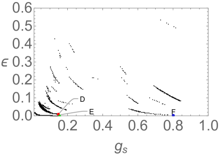
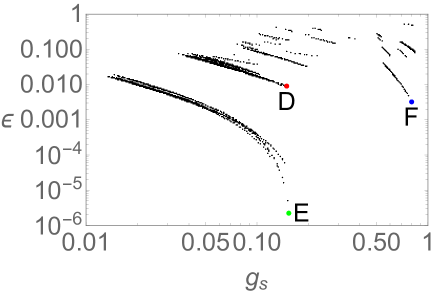
Figure 3: Numerical results for the distribution of non-supersymmetric F-theory flux vacua. Each dot represents a solution with different set of fluxes and the ambiguity from SL(2, $\mathbb{Z}$) duality has been deducted. Note that, as in Figure 1, these dots can be degenerated in this 2D plot, due to the existence of other directions of the stabilized moduli $z$ and $z_{1}$. The right figure is the log-log plot of the same results.

As advocated in the previous section, one can see clearly that the scalar potential and other on-shell quantities thus obtained exhibit a monotonic, non-increasing functional behavior over a wide range of parameter $g_{s}$. One can also check that all the numerical solutions in Figure 3 satisfy the condition (2.17), if we take a sufficiently large volume ${\cal V}$, e.g. larger than $\simeq{\cal{O}}(10^{2})$ for the background geometry.

Here we exemplify our numerical results by picking up three independent flux vacua determined by the following set of fluxes:

Vacuum	Set of fluxes $(n_{1},n_{2}n_{3},n_{4},n_{5},n_{6},n_{7},n_{8},n_{9},n_{10},n_{11})$
D	$(0,0,-2,-8,-8,-2,-6,-4,-7,-8,0)$
E	$(0,0,-3,-7,4,1,-2,-7,-7,-8,-2)$
F	$(0,0,-4,1,-10,-10,2,7,-8,6,0)$

These three examples D, E and F are represented in Figure 3 by the red, green and blue points, respectively. Explicit values of stabilized moduli and various on-shell quantities at the each of the vacua are summarized in Tables 3 and 4. Comparing these results as well as the plots of Figure 3 in F-theory setup with those in Type IIB orientifold model in Section 2.2, it appears that within a finite range of background fluxes of the same amount, the model based on F-theory flux compactification equipped with a next-to-leading-order $g_{s}$ correction prefers a smaller value of the vacuum energy. This preference would provide strong motivation for further studies toward the de Sitter model building in the framework of F-theory dealing with the finite string coupling corrections.

Vacuum	$z_{1}$	$z$	$S$	$g_{s}$	$\epsilon$
D	$-0.703+1.00i$	$-0.0908+2.08i$	$-0.275+6.74i$	0.148	$9.37\times 10^{-3}$
E	$-0.181+1.01i$	$0.0584+2.15i$	$-0.461+6.51i$	0.154	$2.16\times 10^{-6}$
F	$0.243+1.01i$	$0.435+2.03i$	$-0.354+1.25i$	0.802	$3.30\times 10^{-3}$

Table 3: Explicit values of stabilized moduli and on-sell quantities in $M_{\rm Pl}=1$ unit.

Vacuum	$W$	Eigenvalues of mass matrix $\partial_{I}\partial_{J}V\times{\cal V}^{2}$
D	$16.9-32.0i$	(5.13, 2.13, 1.85, 1.26, 0.0446, $2.01\times 10^{-4}$)
E	$-9.16-33.8i$	(3.99, 3.83, 2.89, 1.42, 0.0393, $1.54\times 10^{-6}$ )
F	$25.9+2.33i$	(7.24, 4.56, 3.27, 0.509, 0.154, $7.06\times 10^{-3}$)

Table 4: Explicit values of flux superpotential and mass eigenvalues in $M_{\rm Pl}=1$ unit. Note that we have diagonalized the mass matrix and the eigenvalues are displayed in the descending order.

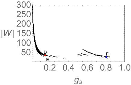
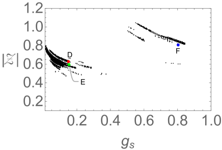
Figure 4: Numerical results for the absolute values of the flux superpotential $|W|$ and $|{\cal Z}|=e^{K/2}|W|$ on each of the flux vacua depicted in Figure 3.

Before ending this section, we would like to discuss about a possible extension of our F-theory setup toward the stabilization of K$\ddot{{\textrm{a}}}$hler moduli and explicit construction of de Sitter spacetime. As can be seen from Figure 4, the absolute value of the superpotential is of, at lowest, ${\cal O}(10)$. This implies that LVS-type extension is more desirable to construct an explicit de Sitter spacetime, rather than utilizing the KKLT-type construction which generically requires an extremely small on-shell value of the flux superpotential. Suppose we employ the LVS-type argument when we extend the K$\ddot{{\textrm{a}}}$hler moduli sector in our F-theory setup, and assume that quantum corrections for K$\ddot{{\textrm{a}}}$hler moduli fields breaking the no-scale structure give rise to a potential

$$V\sim-e^{-\ln\left(2\widetilde{Y}{\rm Im}S\right)}|W_{0}|\frac{\ln{\cal V}}{{\cal V}^{3}}.$$ (3.18)

Then the dimensionless constant $\epsilon$ determined in the dynamics of complex structure moduli sector is further constrained to satisfy a condition $\epsilon\sim e^{K_{\rm CS}}|W_{0}|{\cal V}^{-1}\ln{\cal V}$ such that the total effective potential becomes close to zero as a candidate of the tiny cosmological constant. Since the numerical value of $\epsilon$ obtained in our analysis is sufficiently small to realize this naive expectation, it would be interesting to cast this idea in a rigorous setup.

4 Flux Vacua and Attractor Equations

So far we have analyzed the vacuum structure of effective theories of moduli fields arising from Type IIB and F-theory flux compactifications, aiming to construct appropriate 4D spacetime describing our universe in a consistent and systematic way. There we have shown that the on-shell quantities such as vacuum energy and flux superpotential exhibit a monotonic, non-increasing functional behavior with respect to the string coupling. While this indication strongly motivates us to devote special attention to the significance of F-theory framework for the de Sitter model building, at the same time the following natural question arises: how exactly and why these on-shell quantities on the flux vacua in moduli stabilization problem are determined to exhibit this fascinating behavior?

Here we argue that our findings are deeply connected with a seemingly different topic in the 4D supergravity referred to as the attractor mechanism [40] (see also [41, 42]), where the normalized flux superpotential ${\cal Z}=e^{K/2}W$ of a system can be identified as a central charge of the underlying algebra which is subject to a monotonic flow along the radial direction of a background. More precisely, the attractor mechanism means that in a class of extremal black holes in 4D ${\cal N}=2$ theories, moduli fields are drawn to fixed values at the horizon, regardless of the initial values at the asymptotic infinity. There the fixed values of the moduli fields are determined by the so-called attractor equation. In fact, a possible existence of a correspondence between flux vacua in moduli stabilization and the attractor mechanism in supergravity has been pointed out in [11] (see also [12, 13, 14, 15, 16]). From this perspective, the systematic behavior of various quantities at the distributed flux vacua we observed may reflect the dynamics of a corresponding attracting object, if this kind of correspondence truly exists. Here we provide a supporting evidence for this conjecture by confirming that various solutions we obtained indeed satisfy the suitably generalized attractor equations simultaneously.

First let us reconsider the $T^{6}/\mathbb{Z}_{2}$ toroidal orientifold model as a limit of F-theory on an uplifted fourfold $T^{6}\times T^{2}/\mathbb{Z}_{2}$, in accordance with a prescription illustrated in [11, 12]. Seen from this perspective, the K$\ddot{{\textrm{a}}}$hler potential and flux superpotential in the isotropic case with moduli fields $\Phi_{I}=\{\tau,S\}$ in Section 2.1 can be derived from the generic formulas (3.5) and (3.8) in F-theory compactifications with the following assignment of the fourfold periods

$$\begin{split}\Pi_{1}&=1,\ \Pi_{2}=-S,\ \Pi_{3}=\tau,\ \Pi_{4}=-S\tau,\\ \Pi_{5}&=3\tau^{2},\ \Pi_{6}=-3S\tau^{2},\ \Pi_{7}=-\tau^{3},\ \Pi_{8}=S\tau^{3},\end{split}$$ (4.1)

and the intersection matrix

$$\eta=\begin{pmatrix}0&0&0&0&0&0&0&1\\ 0&0&0&0&0&0&-1&0\\ 0&0&0&0&0&1&0&0\\ 0&0&0&0&-1&0&0&0\\ 0&0&0&-1&0&0&0&0\\ 0&0&1&0&0&0&0&0\\ 0&-1&0&0&0&0&0&0\\ 1&0&0&0&0&0&0&0\end{pmatrix},$$ (4.2)

where the background three-form fluxes in the $T^{6}/\mathbb{Z}_{2}$ model can be reproduced from (3.7) with

$$\vec{n}=\int G_{4}=(-c^{0},a^{0},-c^{1},a_{1},-3d_{1},-3b_{1},d_{0},-b_{0})^{T}.$$ (4.3)

The above reformulation corresponds to geometrize the SL(2, $\mathbb{Z}$) duality of Type IIB string theory into an auxiliary two-torus and combine the various three-forms in Section 2.1 with additional cohomology classes dual to the A- and B-cycles of the torus.

By using above quantities and the central charge ${\cal{Z}}(\tau,\bar{\tau},S,\bar{S})=e^{\frac{K}{2}}W(\tau,S)$, one can check that the Minkowski solutions given by (2.12) and (2.14) of the effective potential also satisfy the attractor equation of a generalized form [11, 43]

$$n_{i}=2{\textrm{Re}}\left[\overline{{\cal{Z}}}\hat{\Pi}_{i}+\overline{D}^{\tau}\overline{D}^{S}\overline{{\cal{Z}}}D_{\tau}D_{S}\hat{\Pi}_{i}\right],$$ (4.4)

where $\overline{D}^{I}\equiv K^{I\bar{J}}{\overline{D}}_{\bar{J}}$ and we have K$\ddot{{\textrm{a}}}$hler-normalized the periods as $\hat{\Pi}_{i}\equiv e^{K/2}\Pi_{i}$. The appearance of this equation can be also understood from the viewpoint of the Hodge structure of allowed four-forms of the system [43]. In a similar fashion, we numerically checked that the non-supersymmetric flux vacua with nonzero scalar potential described in Section 2.2 also satisfy the equation

$$n_{i}=2{\textrm{Re}}\left[\overline{{\cal{Z}}}\hat{\Pi}_{i}-\overline{D}^{I}\overline{{\cal{Z}}}D_{I}\hat{\Pi}_{i}+\overline{D}^{\tau}\overline{D}^{S}\overline{{\cal{Z}}}D_{\tau}D_{S}\hat{\Pi}_{i}\right].$$ (4.5)

More precisely, we have picked up several points in Figure 1 as well as the points A, B and C and confirmed that in all the examples the equation indeed holds up to the accuracy ${\cal{O}}(10^{-20})$, as far as we investigated.

Before moving on to the analysis about F-theory example, we would like to mention that a whole picture of a possible correspondence between flux vacua and attractor mechanism is not completely elucidated even in a simple situation in Type IIB compactification as we actualized above. The main problem is the lack of knowledge about the identification of the exact metric of a corresponding black object, from which the attractor behavior and the entropy can be extracted to confirm the coincidence with the analysis of the flux vacua. Although we naively expect that a warped geometry in 10D spacetime with appropriate fluxes and horizon topology would be relevant, a detailed study of this subject is beyond the scope of the present paper. The simple $T^{6}/\mathbb{Z}_{2}$ toroidal orientifold with a suitable set of background fluxes we thoroughly investigated here may be regarded as a moderate starting point to address this important problem.

Finally, let us discuss about more nontrivial check concerning the F-theory model discussed in Section 3, equipped with the moduli fields $\Phi_{I}=\{z,z_{1},S\}$. After a careful calculation utilizing the fourfold periods (3.9) and the central charge ${\cal{Z}}(z,\bar{z},z_{1},\bar{z_{1}},S,\bar{S})=e^{\frac{K}{2}}W(z,z_{1},S)$, one can check that the Minkowski solution in (3.16) simultaneously satisfies the attractor equation of the following form

$$n_{i}=2{\textrm{Re}}\left[\overline{{\cal{Z}}}\hat{\Pi}_{i}+C^{IJ}D_{I}D_{J}\hat{\Pi}_{i}\right],$$ (4.6)

where $C^{IJ}$ is determined by a condition

$$\overline{D}_{\bar{K}}\overline{D}_{\bar{L}}\overline{Z}=C^{IJ}\biggl{[}R_{I\bar{K}J\bar{L}}+K_{I\bar{K}}K_{J\bar{L}}+K_{I\bar{L}}K_{J\bar{K}}\biggl{]}+\overline{C}^{\bar{I}\bar{J}}e^{K}\overline{Y}_{\bar{I}\bar{J}\bar{K}\bar{L}}.$$ (4.7)

Here $Y_{IJKL}$ represent the classical quadruple intersection numbers of the background Calabi-Yau fourfold whose explicit values can be easily extracted from (3.12), and $R_{I\bar{J}K\bar{L}}$ is the Riemann curvature tensor of the complex structure moduli space defined by

$$R_{I\bar{J}K\bar{L}}=K^{M\bar{N}}(\partial_{\bar{L}}\partial_{\bar{J}}\partial_{M}K)\partial_{I}\partial_{\bar{N}}\partial_{K}K-\partial_{\bar{L}}\partial_{I}\partial_{\bar{J}}\partial_{K}K.$$ (4.8)

Note that the covariant derivative $D_{I}$ appearing in (4.6) and (4.7) is not a simple K$\ddot{{\textrm{a}}}$hler covariant derivative, but also includes the information about the curvature of the moduli space as symbolically represented by $D=\partial+a\partial K+\Gamma.$ Here $a$ is the K$\ddot{{\textrm{a}}}$hler weight of a quantity the covariant derivative acts on, and $\Gamma$ denotes the Christoffel symbol of the second kind of the moduli space metric. For the case of $T^{6}/\mathbb{Z}_{2}$ model discussed above, $\Gamma$ is exactly zero and therefore can be identified with the ordinary K$\ddot{{\textrm{a}}}$hler covariant derivative.

Moreover, we numerically checked that, up to the accuracy ${\cal{O}}(10^{-20})$, the non-supersymmetric flux vacua with nonzero scalar potential found in Section 3.2 satisfy the equation

$$n_{i}=2{\textrm{Re}}\left[\overline{{\cal{Z}}}\hat{\Pi}_{i}-\overline{D}^{I}\overline{{\cal{Z}}}D_{I}\hat{\Pi}_{i}+C^{IJ}D_{I}D_{J}\hat{\Pi}_{i}\right],$$ (4.9)

where the coefficient $C^{IJ}$ is constrained to satisfy (4.7). These results strongly support a possible existence of a F-theory generalization of the attractor mechanism, going beyond the conventional Type IIB setup. Especially, all the explicit results we have shown in the F-theory setup should be regarded as a prediction that if there exists a black object exhibiting the attracting behavior in the framework of F-theory dealing with finite string coupling, its Bekenstein-Hawking entropy and other on-shell quantities would have the same characteristics we have demonstrated above.

5 Conclusions and Discussions

In this paper, we studied several aspects of moduli stabilization in the framework of spacetime flux compactifications by explicitly constructing flux vacua and analyzing their characteristics. Especially we thoroughly investigated the 4D effective theories arising from Type IIB string theory on a toroidal orientifold $T^{6}/\mathbb{Z}_{2}$ and F-theory on a Calabi-Yau fourfold with appropriately quantized background fluxes. As well as clarifying the Minkowski minima with vanishing scalar potential analytically, we numerically solved the extremal conditions of the moduli fields and confirmed that the richness of the choice of background fluxes leads to the existence of vast numbers of stable non-supersymmetric minima of the potential with sufficiently tiny vacuum energy.

Moreover, it turned out that the allowed values of the potential minima and various on-shell quantities show a non-increasing functional behavior with respect to the string coupling $g_{s}$. In particular it appears that within a finite range of background fluxes of the same amount, F-theory model equipped with a next-to-leading-order $g_{s}$ correction prefers a smaller value of the vacuum energy, compared with the simple Type IIB toroidal orientifold model. We hope that several extensions of our results would enrich the stringy construction of the de Sitter spacetime.

We also argued that an interesting conclusion follows from the suggestive behavior of on-shell quantities of Type IIB string and F-theory flux vacua. In the process of clarifying the underlying dynamics of the non-increasing functional behavior of the vacuum energy and the superpotential, we come up with a conclusion that the previously-reported possible correspondence between flux vacua in moduli stabilization problem and attractor mechanism in supergravity lies behind. To provide a nontrivial evidence for this surmise, we have also checked that our analytic and numerical solutions in various flux backgrounds indeed satisfy the suitably generalized attractor equations simultaneously. Especially, our demonstrations in F-theory framework go beyond the conventional Type IIB setups describing the attractor mechanism and may shed new light on this intriguing subject.

Finally, we comment on several possible future research directions in a random order.

• Our studies and demonstrations about the vacuum structure of effective theories would be straightforwardly applicable to broader class of examples based on other type of toroidal orientifolds such as $T^{6}/(\mathbb{Z}_{2}\times\mathbb{Z}_{2})$ [44, 45] and various Calabi-Yau manifolds. Besides providing concrete examples of moduli stabilizations toward the explicit de Sitter model building, this would be connected with a further development of the attractor mechanism in various setups. Within this context, the recent works about asymptotic flux compactifications in [46] and attractor black holes in [47] can be also involved.

• Since our analysis has been restricted to the complex structure moduli as well as the dilaton in Type IIB language, it is indispensable to address the dynamics of the Kähler moduli and their stabilization at the quantum level if one wants to find a landscape of explicit de Sitter minima. As has been emphasized for instance in [48], it will be required to perform a careful analysis with respect to the consistency with the Einstein equations of motion in order to realize the de Sitter spacetime correctly, which should be a highly nontrivial task.

• We naively guess that the standard monotonic gradient flow of the central charge of ordinary attracting extremal BH with respect to the radial direction of a background in SUGRA might be extended at the finite string coupling regime such that the central charge or its derivatives related to the vacuum energy will become also a function of string coupling, whose dependence becomes monotonic if the radial evolution or energy scale in AdS/CFT context and the string coupling are also monotonically correlated. Clarifying this point would be an interesting but highly difficult problem.

• The attractor mechanism states that the evolution of moduli fields is governed by the gradient flow in the radial direction of the 4D background and the central charge ${\cal{Z}}$. On the other hand, it has been recently pointed out that there exists a close relation between the swampland argument and the gradient flow in gravity [49]. Therefore, naively one can expect that our findings about the appearance of the attractor equations in both of the Type IIB string and F-theory flux compactifications might be connected with the basics of the swampland hypothesis. It would be interesting to figure out a more complete description about this expectation.

• About KKLT construction, recent analysis in [50] about the conifold modulus parametrizing the size of three-cycle on the bottom of a warped deformed conifold throat indicates that one must require a large amount of three-form background fluxes to avoid the destabilization, which is generically incompatible with the tadpole cancellation condition in Type IIB flux compactifications. It would be interesting to clarify whether F-theory framework we studied can provide one way to resolve this destabilization problem.

Acknowledgements

We would like to thank K. Ohta, A. Otsuka, K. Sakai and T. Watari for useful discussions and comments. H. O. was supported by a Grant-in-Aid for JSPS Research Fellow No. 19J00664. We appreciate the Yukawa Institute for Theoretical Physics at Kyoto University, where this work was presented during the YITP-W-19-10 on “Strings and Fields 2019”. We are also grateful to the participants of the workshop “KEK Theory Workshop 2018” held at KEK Theory Center for illuminating discussions.

Appendix A Hodge Structure and Attractor Equation

We have described a F-theory generalization of the attractor equation in (4.6) with a condition (4.7). Here let us explain how we arrived at these expressions. In fact, a slight modification of the analysis in [43] leads us to find out appropriate form of the equation.

Along the line of [43] (see also [15]), here we consider an expansion of a generic real four-form flux on a Calabi-Yau fourfold $X_{4}$ as

$$G_{4} =A\hat{\Omega}+B^{I}D_{I}\hat{\Omega}+C^{IJ}D_{I}D_{J}\hat{\Omega}+\overline{A}\overline{\hat{\Omega}}+{\overline{B}}^{\bar{I}}\overline{D}_{\bar{I}}\overline{\hat{\Omega}}+{\overline{C}}^{\bar{I}\bar{J}}\overline{D}_{\bar{I}}\overline{D}_{\bar{J}}\overline{\hat{\Omega}},$$ (A.1)

where the indices $I,J$ label the complex structure moduli of a Calabi-Yau fourfold $X_{4}$, and we have K$\ddot{{\textrm{a}}}$hler-normalized the holomorphic four-form as $\hat{\Omega}(\Phi_{I},\overline{\Phi}_{\bar{I}})\equiv e^{K/2}\Omega(\Phi_{I})$ such that the covariant derivative would acts on $\hat{\Omega}$ as $D_{I}\hat{\Omega}=(\partial_{I}+K_{I}/2)\hat{\Omega}=e^{K/2}D_{I}\Omega$. Let us denote the intersection products of the covariant derivatives of $\hat{\Omega}$ as

$$\begin{split}{\cal N}_{I...J|K...L}&\equiv D_{I}\cdots D_{J}\hat{\Pi}\;\eta^{-1}D_{K}\cdots D_{L}\overline{\hat{\Pi}}=\int_{X_{4}}D_{I}\cdots D_{J}\hat{\Omega}\wedge D_{K}\cdots D_{L}\overline{\hat{\Omega}},\\ {\cal N}^{\prime}_{I...J|K...L}&\equiv D_{I}\cdots D_{J}\hat{\Pi}\;\eta^{-1}D_{K}\cdots D_{L}\hat{\Pi}=\int_{X_{4}}D_{I}\cdots D_{J}\hat{\Omega}\wedge D_{K}\cdots D_{L}\hat{\Omega},\end{split}$$ (A.2)

where we have K$\ddot{{\textrm{a}}}$hler-normalized the fourfold periods of $X_{4}$ as $\hat{\Pi}\equiv e^{K/2}\Pi$. Their explicit forms are known to be given by (see for instance [43])

$$\begin{split}{\cal N}_{I|\bar{J}}&=-K_{I\bar{J}},\\ {\cal N}_{IJ|\bar{K}\bar{L}}&=R_{I\bar{K}J\bar{L}}+K_{I\bar{K}}K_{J\bar{L}}+K_{I\bar{L}}K_{J\bar{K}},\\ {\cal N}_{\bar{I}J|K\bar{L}}&=K_{J\bar{I}}K_{K\bar{L}},\\ {\cal N}^{\prime}_{IJ|KL}&=e^{K}Y_{IJKL},\end{split}$$ (A.3)

where $Y_{IJKL}$ represent classical quadruple intersection numbers of $X_{4}$, and $R_{I\bar{J}K\bar{L}}$ is the Riemann curvature tensor of the complex structure moduli space of $X_{4}$.

Utilizing the above formulas, it turns out that the explicit forms of the coefficients $A$ and $B^{I}$ in (A.1) can be determined by

$$\begin{split}\overline{{\cal{Z}}}&=\int G_{4}\wedge\overline{\hat{\Omega}}=A\int\hat{\Omega}\wedge\overline{\hat{\Omega}}=A,\\ \overline{D}_{\bar{I}}\overline{{\cal{Z}}}&=\int G_{4}\wedge\overline{D}_{\bar{I}}\overline{\hat{\Omega}}=B^{J}\int D_{J}\hat{\Omega}\wedge\overline{D}_{\bar{I}}\overline{\hat{\Omega}}=B^{J}(-K_{J\bar{I}}),\end{split}$$ (A.4)

whereas $C^{IJ}$ and its conjugate are constrained to satisfy

$$\begin{split}\overline{D}_{\bar{K}}\overline{D}_{\bar{L}}\overline{{\cal{Z}}}&=\int G_{4}\wedge\overline{D}_{\bar{K}}\overline{D}_{\bar{L}}\overline{\hat{\Omega}}\\ &=C^{IJ}\int D_{I}D_{J}\hat{\Omega}\wedge\overline{D}_{\bar{K}}\overline{D}_{\bar{L}}\overline{\hat{\Omega}}+\overline{C}^{\bar{I}\bar{J}}\int\ \overline{D}_{\bar{I}}\overline{D}_{\bar{J}}\overline{\hat{\Omega}}\wedge\overline{D}_{\bar{K}}\overline{D}_{\bar{L}}\overline{\hat{\Omega}}\\ &=C^{IJ}\biggl{[}R_{I\bar{K}J\bar{L}}+K_{I\bar{K}}K_{J\bar{L}}+K_{I\bar{L}}K_{J\bar{K}}\biggl{]}+\overline{C}^{\bar{I}\bar{J}}e^{K}\overline{Y}_{\bar{I}\bar{J}\bar{K}\bar{L}}.\end{split}$$ (A.5)

By plugging (A.4) into (A.1) and regarding (A.5) as an additional condition, one can obtain the formulas about the attractor equations discussed in Section 4.

In a generic Type IIB Calabi-Yau compactification, the special K$\ddot{{\textrm{a}}}$hler geometry relation of an underlying Calabi-Yau threefold yields a simplification of the form $D_{i}D_{j}\hat{\Omega}=iY_{ijk}K^{k\bar{l}}D_{\bar{l}}\overline{\hat{\Omega}}$ with $Y_{ijk}$ being classical triple intersection numbers of the threefold with moduli fields $\Phi_{i}$. This makes the basis $D_{i}D_{j}\hat{\Omega}$ in an analogous expansion of a real three-form flux in Type IIB compactifications redundant and as a result the attractor equation in conventional Type IIB setups takes a quite simple form. By contrast, the F-theory compactification based on a generic Calabi-Yau fourfold does not have such a simple structure of special K$\ddot{{\textrm{a}}}$hler geometry and the basis $D_{I}D_{J}\hat{\Omega}$ becomes independent. This is the main reason why a slight modification to the attractor equation is necessary in F-theory framework.

References

- [1] C. Vafa, Nucl. Phys. B 469, 403 (1996) [hep-th/9602022].
- [2] S. B. Giddings, S. Kachru and J. Polchinski, Phys. Rev. D 66 (2002) 106006 [hep-th/0105097].
- [3] S. Gukov, C. Vafa and E. Witten, Nucl. Phys. B 584, 69 (2000) Erratum: [Nucl. Phys. B 608, 477 (2001)] [hep-th/9906070].
- [4] K. Dasgupta, G. Rajesh and S. Sethi, JHEP 9908, 023 (1999) [hep-th/9908088].
- [5] S. Kachru, R. Kallosh, A. D. Linde and S. P. Trivedi, Phys. Rev. D 68 (2003) 046005 [hep-th/0301240].
- [6] V. Balasubramanian, P. Berglund, J. P. Conlon and F. Quevedo, JHEP 0503 (2005) 007 [hep-th/0502058].
- [7] J. P. Conlon, F. Quevedo and K. Suruliz, JHEP 0508 (2005) 007 [hep-th/0505076].
- [8] A. Saltman and E. Silverstein, JHEP 0411 (2004) 066 [hep-th/0402135].
- [9] D. Gallego, M. C. D. Marsh, B. Vercnocke and T. Wrase, JHEP 1710 (2017) 193 [arXiv:1707.01095 [hep-th]].
- [10] J. Blåbck, U. H. Danielsson, G. Dibitetto and S. C. Vargas, JHEP 1510 (2015) 069 [arXiv:1505.04283 [hep-th]].
- [11] R. Kallosh, JHEP 0512, 022 (2005) [hep-th/0510024].
- [12] R. Kallosh, hep-th/0509112.
- [13] R. Kallosh, N. Sivanandam and M. Soroush, JHEP 0603, 060 (2006) [hep-th/0602005].
- [14] M. Alishahiha and H. Ebrahim, JHEP 0611, 017 (2006) [hep-th/0605279].
- [15] S. Bellucci, S. Ferrara, R. Kallosh and A. Marrani, Lect. Notes Phys. 755, 115 (2008) [arXiv:0711.4547 [hep-th]].
- [16] F. Larsen and R. O’Connell, JHEP 0907, 049 (2009) [arXiv:0905.2130 [hep-th]].
- [17] S. Kachru, M. B. Schulz and S. Trivedi, JHEP 0310 (2003) 007 [hep-th/0201028].
- [18] A. R. Frey and J. Polchinski, Phys. Rev. D 65, 126009 (2002) [hep-th/0201029].
- [19] R. D’Auria, S. Ferrara and S. Vaula, New J. Phys. 4, 71 (2002) [hep-th/0206241].
- [20] A. R. Frey and A. Mazumdar, Phys. Rev. D 67, 046006 (2003) [hep-th/0210254].
- [21] M. Dine and N. Seiberg, Phys. Lett. 162B, 299 (1985).
- [22] G. Obied, H. Ooguri, L. Spodyneiko and C. Vafa, arXiv:1806.08362 [hep-th].
- [23] S. K. Garg and C. Krishnan, arXiv:1807.05193 [hep-th].
- [24] H. Ooguri, E. Palti, G. Shiu and C. Vafa, Phys. Lett. B 788, 180 (2019) [arXiv:1810.05506 [hep-th]].
- [25] Y. Honma and H. Otsuka, Phys. Lett. B 774 (2017) 225 [arXiv:1706.09417 [hep-th]].
- [26] K. Becker and M. Becker, Nucl. Phys. B 477, 155 (1996) [hep-th/9605053].
- [27] S. Sethi, C. Vafa and E. Witten, Nucl. Phys. B 480, 213 (1996) [hep-th/9606122].
- [28] M. Haack and J. Louis, Phys. Lett. B 507, 296 (2001) [hep-th/0103068].
- [29] F. Denef, Les Houches 87, 483 (2008) [arXiv:0803.1194 [hep-th]].
- [30] M. Alim, M. Hecht, H. Jockers, P. Mayr, A. Mertens and M. Soroush, Nucl. Phys. B 841, 303 (2010) [arXiv:0909.1842 [hep-th]].
- [31] T. W. Grimm, T. W. Ha, A. Klemm and D. Klevers, JHEP 1004, 015 (2010) [arXiv:0909.2025 [hep-th]].
- [32] H. Jockers, P. Mayr and J. Walcher, Adv. Theor. Math. Phys. 14, no. 5, 1433 (2010) [arXiv:0912.3265 [hep-th]].
- [33] T. W. Grimm, A. Klemm and D. Klevers, JHEP 1105, 113 (2011) [arXiv:1011.6375 [hep-th]].
- [34] Y. Honma and M. Manabe, JHEP 1603, 160 (2016) [arXiv:1507.08342 [hep-th]].
- [35] Y. Honma and M. Manabe, JHEP 1305, 102 (2013) [arXiv:1302.3760 [hep-th]].
- [36] T. W. Grimm, R. Savelli and M. Weissenbacher, Phys. Lett. B 725 (2013) 431 [arXiv:1303.3317 [hep-th]].
- [37] T. W. Grimm, J. Keitel, R. Savelli and M. Weissenbacher, Nucl. Phys. B 903 (2016) 325 [arXiv:1312.1376 [hep-th]].
- [38] R. Minasian, T. G. Pugh and R. Savelli, JHEP 1510, 050 (2015) [arXiv:1506.06756 [hep-th]].
- [39] M. Weissenbacher, arXiv:1901.04758 [hep-th].
- [40] S. Ferrara, R. Kallosh and A. Strominger, Phys. Rev. D 52, R5412 (1995) [hep-th/9508072].
- [41] S. Ferrara, K. Hayakawa and A. Marrani, Fortsch. Phys. 56, 993 (2008) [arXiv:0805.2498 [hep-th]].
- [42] G. W. Moore, hep-th/0401049.
- [43] F. Denef and M. R. Douglas, JHEP 0405 (2004) 072 [hep-th/0404116].
- [44] R. Blumenhagen, D. Lust and T. R. Taylor, Nucl. Phys. B 663, 319 (2003) [hep-th/0303016].
- [45] J. F. G. Cascales and A. M. Uranga, JHEP 0305, 011 (2003) [hep-th/0303024].
- [46] T. W. Grimm, C. Li and I. Valenzuela, arXiv:1910.09549 [hep-th].
- [47] G. Hulsey, S. Kachru, S. Yang and M. Zimet, arXiv:1901.10614 [hep-th].
- [48] K. Dasgupta, R. Gwyn, E. McDonough, M. Mia and R. Tatar, JHEP 1407 (2014) 054 [arXiv:1402.5112 [hep-th]].
- [49] A. Kehagias, D. Lst and S. Lst, arXiv:1910.00453 [hep-th].
- [50] I. Bena, E. Dudas, M. Graa and S. Lst, Fortsch. Phys. 67 (2019) no.1-2, 1800100 [arXiv:1809.06861 [hep-th]].