Parking 3-sphere swimmer
II. The long arm asymptotic regime

Abstract. The paper carries on our previous investigations on the complementary version of Purcell’s rotator (spr₃): a low-Reynolds-number swimmer composed of three balls of equal radii. In the asymptotic regime of very long arms, the Stokes induced governing dynamics is derived, and then experimented in the context of energy minimizing self-propulsion characterized in the first part of the paper.

1. Introduction

In his seminal paper [16], Purcell explains how at small Reynolds numbers any organism trying to swim using the reciprocal stroke of a scallop, which moves by opening and closing its valves, is condemned to go back to its original position at the end of one cycle. This observation leads to the question of finding the simplest mechanisms capable of self-propulsion at these scales; by this, we mean the ability to moving by performing a cyclic shape change, a stroke, in the absence of external forces. Several proposals have been put forward and analyzed (see, e.g., [6, 7, 13, 15, 16, 18] and the review paper [12]).

In this paper, we focus on a very specific microswimmer: the complementary version of Purcell’s three-sphere rotator (spr₃) introduced in [13] and fully described in Section 2. This swimmer consists of three non-intersecting balls $(B_{i})_{i\in\mathbbmss{N}_{3}}$ of $\mathbbmss{R}^{3}$ centered at $b_{i}\in\mathbbmss{R}^{3}$ and of equal radii $a>0$ (for $n\in\mathbbmss{N}$ we set $\mathbbmss{N}_{n}:=\{1,\ldots,n\}$). The three balls can move along three coplanar axes that mutually meet at a point $c\in\mathbbmss{R}^{3}$, the center, with fixed angles of $2\pi/3$ one to another; this reflects a situation where the balls are linked together by very thin telescopic arms that can elongate (see Figure 1). The swimmer can freely rotate around $c$ in the horizontal plane containing the arms, although owing to the symmetries of the system, it is forced to stay in this plane.

Full controllability of spr₃, as well as for a broader class of model swimmers, i.e., the ability of the swimmer to reach any point in the plane with any orientation, has been proved in [4], while analytical investigations on the optimal control problem have been the object of [5]. Compared to [4, 5], we propose here a quantitative analysis and we want to stress that, by contrast to the earlier works on the topic (cf. [1, 2, 3, 6, 7, 8, 9, 15, 16, 17]), here the presence of three control variables and three position variables makes the analysis more involved and rich.

The main aim of this second part is to put the optimality results proved in [5] into a concrete setting, specifically: the Stokes induced governing control system for spr₃ in the asymptotic regime of very long arms. First, we derive closed-form expressions for the dynamics and use asymptotic analysis to simplify the results. Then, we focus on the analysis of energy-minimizing strokes, and we identify the optimal parameters of the control system in terms of the initial length of the arms and the radius of the three balls. Finally, we present numerical simulations that show the qualitative features of the optimal swimming style.

2. Kinematics and Dynamics of spr₃

As the three balls are not allowed to rotate around their axes, the shape of the swimmer can be parametrized by the lengths $\zeta_{1},\zeta_{2},\zeta_{3}$ of its three arms, measured from $c$ to the center of each of the balls. Therefore, the possible geometrical configurations of the swimmer can be described by introducing two sets of variables:

• The vector of shape variables $\zeta{\color[rgb]{0,0,0}{:=}}\left(\zeta_{1},\zeta_{2},\zeta_{3}\right)\in\mathcal{M}{\color[rgb]{0,0,0}{:=}}\left(2a/\sqrt{3},\infty\right)^{3}\subseteq\mathbbmss{R}_{+}^{3}$ from which relative distances $(b_{ij})_{i,j\in\mathbbmss{N}_{3}}$ between the balls are obtained (cf. (2) and (3)). The lower bound on $\mathcal{M}$ is imposed to exclude any overlap of the spheres.

• Position and orientation of spr₃ in the plane are specified by the coordinates of the center $c\in\mathbbmss{R}^{2}\times\{0\}$, and by the angle $\theta$ that one arm, e.g., the arm connected to $B_{1}$, makes with the fixed direction $z_{1}$. We refer to $p=(c,\theta)\in\mathbbmss{R}^{2}\times\mathbbmss{R}$ as the vector of position variables.

Precisely, without loss of generality, we assume that in its initial configuration, the three arms of the swimmer sit in the plane $\mathbbmss{R}^{2}\times\{0\}$. In order to compute the position of the three balls, we take the vertices of the equilateral triangle defined as the convex hull of the unit vectors $z_{1},z_{2},z_{3}\in\mathbbmss{R}^{3}$, with $z_{1}:=(1,0,0)^{\mathsf{T}}$, $z_{2}:=R^{\mathsf{T}}(2\pi/3)z_{1}$, $z_{3}:=R(2\pi/3)z_{1}$, and $R(\phi)$ the planar rotation through an angle $\phi\in\mathbbmss{R}$ around the vector $\hat{e}_{3}=(0,0,1)$:

$$R(\phi){\color[rgb]{0,0,0}{:=}}\left(\begin{array}[]{ccc}\cos\phi&-\sin\phi&0\\ \sin\phi&\cos\phi&0\\ 0&0&1\end{array}\right).$$ (1)

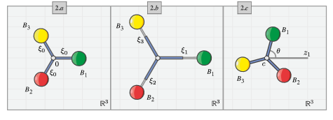
Figure 2. The swimmer spr₃ is fully described by the set of shape variables $\zeta{\color[rgb]{0,0,0}{:=}}\left(\zeta_{1},\zeta_{2},\zeta_{3}\right)\in\mathcal{M}$ and by the set of position variables $p=(c,\theta)\in\mathbbmss{R}^{2}\times\mathbbmss{R}$. [From left to right] In 2. a, the reference configuration. The three spheres are located at the vertices of an equilateral triangle having the origin as barycenter ($c=0$). In 2. b, the set of shape variables $\zeta{\color[rgb]{0,0,0}{:=}}(\xi_{0}+\xi_{1},\xi_{0}+\xi_{2},\xi_{0}+\xi_{3})\in\mathcal{M}$ represents a possible shape state of the swimmer characterized by three different lengths of the arms. In 2. c, a possible position state $(c,\theta)$, with $\theta\neq 0$, is sketched.

Then, the center $b_{i}$ of the $i$-th ball of the swimmer is at position (cf. Figure 2)

$$b_{i}:=c+\zeta_{i}R(\theta)z_{i}\in\mathbbmss{R}^{2},$$ (2)

where, here and in the sequel, we identify $\mathbbmss{R}^{2}$ with $\mathbbmss{R}^{2}\times\{0\}$ and, similarly, we identify the action of $R$ in (1) with its two-dimensional analog. Since the balls cannot intersect, the matrix $b{\color[rgb]{0,0,0}{:=}}(b_{1},b_{2},b_{3})\in\mathbbmss{R}^{2\times 3}$ is constrained to take values into the set

$$\mathcal{B}:=\left\{b\in\mathbbmss{R}^{2\times 3}:\,\min_{i<j\,}|b_{ij}|>2a\right\},\qquad b_{ij}:=b_{i}-b_{j}.$$ (3)

The time evolution of the swimmer can be traced through the state variables $\left(\zeta,p\right)\in\mathcal{M}\times\mathbbmss{R}^{3}$. For $i\in\mathbbmss{N}_{3}$, the instantaneous velocity of the $i$-th sphere is obtained by differentiating relation (2) with respect to time

$$u_{i}\left(\zeta,p\right)=\dot{c}+\dot{\zeta}_{i}R(\theta)z_{i}+\dot{\theta}\zeta_{i}R(\theta)z_{i}^{\bot},$$ (4)

with $z_{i}^{\bot}{\color[rgb]{0,0,0}{:=}}R(\pi/2)z_{i}$.

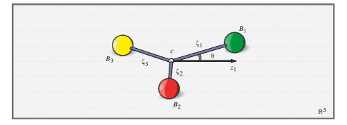
Figure 1. The swimmer spr₃  is composed of three non-intersecting balls $(B_{i})_{i\in\mathbbmss{N}_{3}}$ of $\mathbbmss{R}^{3}$ of equal radii. The three balls are linked together by thin arms that are able to elongate, independently of each other, along three coplanar axes that meet at the center $c\in\mathbbmss{R}^{3}$ and make fixed angles of $2\pi/3$ from one to another.

The viscous resistance of the arms is deemed negligible and, therefore, we assume that the fluid fills up the whole space outside the balls, that is, the exterior domain $\Omega{\color[rgb]{0,0,0}{:=}}\mathbbmss{R}^{3}\backslash\cup_{i=1}^{3}\bar{B}_{i}$. The geometry of $\Omega$ is uniquely determined by the common radius $a$ of the three spheres, and by the matrix $b=(b_{i})_{i\in\mathbbmss{N}_{3}}$ having as columns the centers of the balls. At low Reynolds numbers, the dynamics of the swimmer is governed by the Stokes equations

$$\left\{\begin{array}[]{rll}-\mu\Delta u+\nabla p=&0&\text{in }\Omega,\\ \operatorname{div}u=&0&\text{in }\Omega,\end{array}\right.$$ (5)

where $u$ and $p$ are, respectively, the velocity field and the pressure of the fluid, and $\mu$ is its viscosity. As the structure of the swimmer is deformable but made of rigid balls, the governing equations are subject to no-slip boundary conditions on the balls. Because of the linearity of Stokes equations, the vector $\boldsymbol{u}:=(u_{1},u_{2},u_{3})$ collecting the three velocities in (4) can be expressed in the algebraic form (cf. [11, 15])

$$\boldsymbol{u}=\mathcal{H}\boldsymbol{f},$$ (6)

where $\mathcal{H}$ is the Oseen tensor (which depends on the viscosity) and $\boldsymbol{f}:=(f_{1},f_{2},f_{3})\in\mathbbmss{R}^{6}$ is the vector collecting the forces acting on the balls. Symmetry arguments show that in the long arm asymptotic regime the hydrodynamic relation (6) takes the form:

$$u_{i}=\frac{1}{\nu}f_{i}\;+\sum_{j\neq i\in\mathbbmss{N}_{3}}\mathcal{S}(b_{ij})f_{j}$$ (7)

where the stokeslet

$$\mathcal{S}(x){\color[rgb]{0,0,0}{:=}}\frac{1}{8\pi\mu}\left(\frac{I}{|x|}+\frac{x\otimes x}{|x|^{3}}\right)$$ (8)

represents a fundamental solution of the Stokes system [10], and $\nu:=6\pi\mu a\in\mathbbmss{R}^{+}$ is the drag coefficient linking, at small Reynolds numbers, the force to the velocity of a spherical object of radius $a\in\mathbbmss{R}^{+}$ immersed in a fluid of viscosity $\mu$.

It will be convenient to rewrite (7) in the form

$$\boldsymbol{u}=\left(\frac{1}{\nu}\mathcal{I}+\mathcal{L}\right)\boldsymbol{f},$$ (9)

where $\mathcal{I}:=\operatorname{diag}(I,I,I)$ is the $6\times 6$ identity matrix, and $\mathcal{L}$ the mutual interaction matrix defined by

$$\mathcal{L}:=\left(\begin{array}[]{ccc}0&\mathcal{S}(b_{12})&\mathcal{S}(b_{13})\\ \mathcal{S}(b_{12})&0&\mathcal{S}(b_{23})\\ \mathcal{S}(b_{13})&\mathcal{S}(b_{23})&0\end{array}\right).$$ (10)

3. Dynamics of spr₃ in the limit of very long arms

Due to the negligible inertia, the total viscous force and torque exerted by the surrounding fluid on the swimmer must vanish. In other words, the dynamics is subject to the balance equations

$$\sum_{i\in\mathbbmss{N}_{3}}f_{i}=0\quad\text{and}\quad\sum_{i\in\mathbbmss{N}_{3}}b_{i}\times f_{i}=0.$$ (11)

Here, the cross product stands for the determinant form on $\mathbbmss{R}^{2}$ and the $b_{i}$’s are given by (2). Clearly, for every $i\in\mathbbmss{N}_{3}$, there exist vectors $b_{\bot,i}(\zeta_{i},\theta)\in\mathbbmss{R}^{2}$, such that $b_{\bot,i}(\zeta_{i},\theta)\cdot f_{i}=b_{i}\times f_{i}$, and, therefore, the balance equations (11) can be expressed in the concise form

$$\mathcal{W}(\zeta,\theta)\boldsymbol{f}=0,$$ (12)

where the matrix $\mathcal{W}$ is defined by

$$\mathcal{W}(\zeta,\theta):=\left(\begin{array}[]{ccc}I_{2\times 2}&I_{2\times 2}&I_{2\times 2}\\[2.0pt] b_{\bot,1}^{\mathsf{T}}(\zeta_{1},\theta)&b_{\bot,2}^{\mathsf{T}}(\zeta_{2},\theta)&b_{\bot,3}^{\mathsf{T}}(\zeta_{3},\theta)\end{array}\right).$$ (13)

We assume that the three arms of the swimmer have the same initial length $\xi_{0}\in\mathbbmss{R}^{+}$ with $\xi_{0}\gg a$, and we set $\zeta_{i}:=\xi_{0}+\xi_{i}$ with $|\xi_{i}|\ll\xi_{0}$. We want to show that in the limit of very long arms, and at the leading order, the swimming problem for spr₃ reduces to a control problem of the form

$$\dot{p}\;=F(\xi,\theta)\dot{\xi},$$ (14)

with $\xi:=(\xi_{1},\xi_{2},\xi_{3})$, whose structural symmetries have been fully investigated in the first part of the paper (cf. [5]).

First, since the vector of the velocities depends linearly both on $\dot{\xi}$ and $\dot{p}$, we can recast relations (4) in the form

$$\boldsymbol{u}=\mathcal{X}(\theta)\dot{\xi}+\mathcal{Y}(\xi,\theta)\dot{p}$$ (15)

where $\mathcal{X},\mathcal{Y}$ are the shape matrices given by

$$\begin{array}[]{rll}\mathcal{X}(\theta)&:=&\left(\begin{array}[]{c|c|c}R(\theta)z_{1}&0_{2\times 1}&0_{2\times 1}\\ 0_{2\times 1}&R(\theta)z_{2}&0_{2\times 1}\\ 0_{2\times 1}&0_{2\times 1}&R(\theta)z_{3}\end{array}\right)_{6\times 3},\\[8.0pt] \\ \mathcal{Y}(\xi,\theta)&:=&\left(\begin{array}[]{c|c}I_{2\times 2\;}&(\xi_{0}+\xi_{1})R(\theta)z_{1}^{\bot}\\ I_{2\times 2\;}&(\xi_{0}+\xi_{2})R(\theta)z_{2}^{\bot}\\ I_{2\times 2\;}&(\xi_{0}+\xi_{3})R(\theta)z_{3}^{\bot}\end{array}\right)_{6\times 3}.\end{array}$$ (16)

In the limit of large arms, the mutual interaction matrix becomes a perturbation of the diagonal part $(1/\nu)\mathcal{I}$ and equation (9) can be inverted to give (at the leading order)

$$\boldsymbol{f}=\left(\nu\mathcal{I}-\nu^{2}\mathcal{L}\right)\boldsymbol{u}=\left(\nu\mathcal{I}-\nu^{2}\mathcal{L}\right)\left(\mathcal{X}(\theta)\dot{\xi}+\mathcal{Y}(\xi,\theta)\dot{p}\right)$$ (17)

by use of (15). Multiplying both members by $\mathcal{W}$, and after simplifying by $\nu$, we infer that (cf. (12))

$$\mathcal{W}(\xi,\theta)\left(\mathcal{I}-\nu\mathcal{L}\right)\left(\mathcal{X}(\theta)\dot{\xi}+\mathcal{Y}(\xi,\theta)\dot{p}\right)=0,$$ (18)

with the convenient and not dangerous abuse of notation $\mathcal{W}(\xi,\theta):=\mathcal{W}(\zeta,\theta)$. This is of the desired form (14) with

$$F=-\left(\mathcal{W}\left(\mathcal{I}-\nu\mathcal{L}\right)\mathcal{Y}\right)^{-1}\mathcal{W}\left(\mathcal{I}-\nu\mathcal{L}\right)\mathcal{X}$$ (19)

where, to shorten notation, we left understood the parameters $\xi_{0},\xi$ and $\theta$. Moreover, because of the invariance of Stokes equations under the group of rotations, according to [5] (Prop. 1), we can factorize the control system $F$ in the form $F(\xi,\theta)=R(\theta)F(\xi)$ with $F(\xi):=F(\xi,0)$, and therefore

$$\dot{p}\;=\;R(\theta)F(\xi)\dot{\xi}.$$ (20)

Also (cf. [5] (Prop. 4)), in the limit of small strokes, i.e., in the regime $|\xi|/\xi_{0}<a/\xi_{0}\ll 1$ (see also Section 5), we can expand $F$ to leading order in $\xi$. This gives

$$F(\xi)\dot{\xi}=F_{0}\dot{\xi}+\sum_{k\in\mathbbmss{N}_{3}}(A_{k}\dot{\xi}\cdot\xi)e_{k}.$$ (21)

Here, a straightforward computation shows that $F_{0}:=F(0)$ is given by

$$F_{0}=\varphi(a,\xi_{0})\left(\begin{array}[]{ccc}-2&1&1\\ 0&\sqrt{3}&-\sqrt{3}\\ 0&0&0\end{array}\right),$$ (22)

with

$$\varphi(a,\xi_{0}):=\frac{1}{6}-\frac{1}{16\sqrt{3}}(a/\xi_{0})+\mathcal{O}(a/\xi_{0})^{2}.$$ (23)

Instead, the first order correctors $(A_{k})_{k\in\mathbbmss{N}_{3}}$ (cf. [5] (Corollary 1)) have a special structure which can be fully characterized in terms of four real parameters. Precisely, there exist $\alpha{\color[rgb]{0,0,0}{:=}}\alpha(a,\xi_{0}),\beta{\color[rgb]{0,0,0}{:=}}\beta(a,\xi_{0}),\gamma{\color[rgb]{0,0,0}{:=}}\gamma(a,\xi_{0})$, and $\lambda{\color[rgb]{0,0,0}{:=}}\lambda(a,\xi_{0})$, depending only on the radius $a$ of the balls and on the initial common length $\xi_{0}$ of the arms of spr₃, such that

$$\begin{array}[]{lll}A_{1}&=&\left(\begin{array}[]{ccc}-\lambda&\alpha+\frac{1}{3}\beta&\alpha+\frac{1}{3}\beta\\ -\alpha+\frac{1}{3}\beta&\frac{\lambda}{2}&-\frac{2}{3}\beta\\ -\alpha+\frac{1}{3}\beta&-\frac{2}{3}\beta&\frac{\lambda}{2}\end{array}\right),\\ \\ A_{2}&=&\sqrt{3}\left(\begin{array}[]{ccc}0&\frac{\alpha-\beta}{3}&\frac{\beta-\alpha}{3}\\ \frac{-\beta-\alpha}{3}&\frac{\lambda}{2}&-\frac{2\alpha}{3}\\ \frac{\alpha+\beta}{3}&\frac{2\alpha}{3}&-\frac{\lambda}{2}\end{array}\right),\end{array}$$ (24)

and

$$A_{3}=\left(\begin{array}[]{ccc}0&-\gamma&\gamma\\ \gamma&0&-\gamma\\ -\gamma&\gamma&0\end{array}\right).$$ (25)

With the aid of a symbolic computation software and expanding $F$ in terms of $\xi$ in (19) we can identify the entries and get

$$\alpha(a,\xi_{0}) := \frac{1}{\xi_{0}}\left(\frac{1}{32\sqrt{3}}(a/\xi_{0})+\mathcal{O}(a/\xi_{0})^{2}\right),$$ (26)

$$\beta(a,\xi_{0}) := \frac{1}{\xi_{0}}\left(\frac{1}{16\sqrt{3}}(a/\xi_{0})+\mathcal{O}(a/\xi_{0})^{2}\right),$$ (27)

$$\lambda(a,\xi_{0}) := \frac{1}{\xi_{0}}\left(\frac{5}{48\sqrt{3}}(a/\xi_{0})+\mathcal{O}(a/\xi_{0})^{2}\right),$$ (28)

and

$$\gamma(a,\xi_{0}) := \frac{1}{\xi_{0}^{2}}\left(\frac{1}{6\sqrt{3}}+\mathcal{O}(a/\xi_{0})^{2}\right).$$ (29)

We remark that only the skew-symmetric parts $(M_{k})_{k\in\mathbbmss{N}_{3}}$ of the matrices $(A_{k})_{k\in\mathbbmss{N}_{3}}$ contribute to a net displacement of the swimmer after one stroke (cf. [5]). For any $\xi\in\mathbbmss{R}^{3}$ they can be expressed by the actions

$$M_{1}\xi=\alpha\xi\times\tau_{1},\quad M_{2}\xi=\alpha\xi\times\tau_{2},\quad M_{3}\xi=\gamma\xi\times\tau_{3},$$ (30)

with

$$\tau_{1}{\color[rgb]{0,0,0}{:=}}(0,-1,1),\;\tau_{2}{\color[rgb]{0,0,0}{:=}}\frac{1}{\sqrt{3}}(-2,1,1),\;\tau_{3}{\color[rgb]{0,0,0}{:=}}(1,1,1)$$ (31)

forming an orthogonal basis of $\mathbbmss{R}^{3}$.

4. Optimal swimming

Following the notion of swimming efficiency proposed by Lighthill in [14] (cf. also [9, 17]), we adopt the following notion of kinematic optimality: energy minimizing strokes are those minimizing the kinetic energy dissipated during one stroke in order to reach a prescribed net displacement $\delta p\in\mathbbmss{R}^{3}$. In mathematical terms, the total energy dissipation due to a smooth stroke $\zeta:I\rightarrow\mathcal{M}$, can be evaluated by considering the instantaneous power dissipated at time $t\in I$, defined by $\mathcal{P}(\boldsymbol{u})=\boldsymbol{f}\cdot\boldsymbol{u}$. We note that $\dot{p}$ is linear in $\dot{\xi}$ because of (14), and so are $\boldsymbol{f}$ and $\boldsymbol{u}$ due to (15) and (17). Thus $\mathcal{P}(\boldsymbol{u})$ turns out to be a quadratic form in $\dot{\xi}$ that we write in the following form

$$\mathcal{P}(\boldsymbol{u})=G(\xi)\dot{\xi}\cdot\dot{\xi}$$ (32)

for a suitable matrix-valued function $G$ that, by the rotational invariance of the problem, does not depend on $\theta$.

At the leading order in the limit of small strokes (cf. [5] (§ 5)) the instantaneous power dissipated at time $t\in I$ reads as $\mathcal{P}(\boldsymbol{u}(t))=G_{0}\dot{\xi}(t)\cdot\dot{\xi}(t)$, with $G_{0}:=G(0)$, and the total energy dissipation associated with a stroke $\zeta:I\rightarrow\mathcal{M}$ is given by (recalling that $\zeta_{i}:=\xi_{0}+\xi_{i}$)

$$\mathcal{G}(\zeta){\color[rgb]{0,0,0}{:=}}\int_{I}G_{0}\dot{\xi}(t)\cdot\dot{\xi}(t)\mathrm{d}t.$$ (33)

It can be readily checked that, as derived in [5] (§ 5), the matrix $G_{0}$ is symmetric, positive-definite, and has the following special structure

$$G_{0}=\left(\begin{array}[]{ccc}\kappa&h&h\\ h&\kappa&h\\ h&h&\kappa\end{array}\right),$$ (34)

with the two parameters $h,\kappa$ depending only on the ratio $a/\xi_{0}$ between the radius of the balls of spr₃, and on the common initial length of its arms. Again, a symbolic computation shows that

$$\begin{array}[]{lll}\kappa&:=&\frac{2}{3}+\frac{1}{\sqrt{3}}(a/\xi_{0})+\mathcal{O}(a/\xi_{0})^{2},\\ \\ h&:=&\frac{1}{6}+\frac{7}{16\sqrt{3}}(a/\xi_{0})+\mathcal{O}(a/\xi_{0})^{2}.\end{array}$$ (35)

It is convenient to denote by $g_{1}{\color[rgb]{0,0,0}{:=}}(\kappa-h)$ and $g_{2}{\color[rgb]{0,0,0}{:=}}(\kappa+2h)$ the eigenvalues of $G_{0}$. Note that $g_{1}$ is of multiplicity two. Their expanded expressions read as

$$g_{1} = \frac{1}{2}+\frac{3\sqrt{3}}{16}(a/\xi_{0})+\mathcal{O}(a/\xi_{0})^{2},$$ (36)

$$g_{2} = 1+\frac{5\sqrt{3}}{8}(a/\xi_{0}).$$ (37)

In [5] (Theorem 5.1) we proved that the stroke $\zeta:I\rightarrow\mathcal{M}$ that produces a prescribed change of position and orientation $\delta p\in\mathbbmss{R}^{3}$ of the swimmer at the minimal cost $\mathcal{G}(\zeta)$ is an ellipse of $\mathbbmss{R}^{3}$. This optimal stroke is given by

$$\xi(t){\color[rgb]{0,0,0}{:=}}(\cos t)u+(\sin t)v,$$ (38)

where the vectors $u,v\in\mathbbmss{R}^{3}$ can be fully computed from $\delta p$, the coefficients $\alpha,\gamma$ of the skew-symmetric matrices $(M_{k})_{k\in\mathbbmss{N}_{3}}$, and the eigenvalues of $G_{0}$.

Namely, as shown in [5] (Theorem 5.1), any minimizer is, in $\xi$, an ellipse of $\mathbbmss{R}^{3}$ centered at the origin, and the minimum value of $\mathcal{G}$ is equal to $|\omega|$ where

$$\omega:=\operatorname{diag}\left(\frac{\sqrt{g_{1}g_{2}}}{\sqrt{2}\alpha},\frac{\sqrt{g_{1}g_{2}}}{\sqrt{2}\alpha},\frac{g_{1}}{\sqrt{3}\gamma}\right)\delta p.$$ (39)

More precisely, considering two orthogonal vectors $\varsigma_{1},\varsigma_{2}\in\mathbbmss{R}^{3}$ in the plane orthogonal to $\omega$ and such that $|\varsigma_{1}|^{2}=|\varsigma_{2}|^{2}=|\omega|$, we can compute the vectors $u$ and $v$ in (38) via the relations

$$u{\color[rgb]{0,0,0}{:=}}\frac{U\Lambda^{-1/2}}{\sqrt{2\pi}}\varsigma_{1}\hskip 1.69998pt,\quad v{\color[rgb]{0,0,0}{:=}}\frac{U\Lambda^{-1/2}}{\sqrt{2\pi}}\varsigma_{2},$$ (40)

with $U=(\tau_{i}/|\tau_{i}|)_{i\in\mathbbmss{N}_{3}}$ (cf. (31)) and $\Lambda:=\operatorname{diag}(g_{1},g_{1},g_{2})$.

Summarizing, at the leading order in the range of small strokes and very long arms, the governing dynamics of spr₃ for energy minimizing strokes is given by (cf. (21))

$$\theta(t)=\sigma t\quad\text{with}\quad\sigma{\color[rgb]{0,0,0}{:=}}\gamma(u\times v)\cdot\tau_{3}\in\mathbbmss{R},$$ (41)

$$\dot{c}(t)=R(\sigma t)F_{0}\dot{\xi}(t)+R(\sigma t)\sum_{j\in\mathbbmss{N}_{2}}(A_{j}\dot{\xi}(t)\cdot\xi(t))e_{j},$$ (42)

with $(A_{j})_{j\in\mathbbmss{N}_{2}}$ given by (24), and $u,v\in\mathbbmss{R}^{3}$ given by (40). In particular, the angular velocity of the swimmer is constant in time and is zero when the prescribed net displacement $\delta p$ is purely translational ($\delta p_{3}=0$).

It is easily seen that energy minimizing net displacements along the $x$-axis direction are achieved via elliptic strokes contained in the plane orthogonal to the vector $\tau_{1}$. Similarly pure along-$y$ (resp. along-$\theta$) net displacements are achieved via elliptic strokes contained in the plane orthogonal to $\tau_{2}$ (resp. to $\tau_{3}$).

The results of numerical simulations of (41)-(42) when the control $\zeta$ is the optimal swimming strategy for a prescribed net displacement $\delta p$ along the $x,y$ and $\theta$ directions are shown in Figure 3. Although we put some effort in drawing pictures that give a good feeling of how the swimmer performs, we are aware that the dynamics can be better appreciated by watching a video rather than looking at static frames; in that regard, in the supplementary electronic material, it is possible to find a video demonstrating the motion traced by spr₃ during optimal swimming.

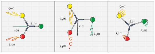
Figure 3. The evolution of $\xi$ and $c$ during optimal strokes. (left) Shape and position changes described by spr₃ to achieve a pure $x$ displacement. (center) Shape and position changes to achieve a pure $y$ displacement. (right) Shape and position changes to achieve a pure $\theta$ displacement.

5. Concluding Remarks

Note that, for $j=1,2$, we have that $\lim_{\xi_{0}\rightarrow\infty}A_{j}(a,\xi_{0})=0$ and $\lim_{a\rightarrow 0}A_{j}(a,\xi_{0})=0$. However, since $\gamma(0,\xi_{0})=1/\left(6\sqrt{3}\xi_{0}^{2}\right)$ and $A_{3}=M_{3}$,

$$\lim_{\xi_{0}\rightarrow\infty}M_{3}(a,\xi_{0})=0,\quad\quad\lim_{a\rightarrow 0}M_{3}(a,\xi_{0})\neq 0.$$ (43)

In other words, the asymptotic limit of very small balls differs from one of very long arms. This is understood by the presence of two fundamental geometric scales: the common radius $a$ of the three balls, and the initial length $\xi_{0}$ of its arms. In this respect, the two following asymptotic regimes are different:

$$\frac{a}{\xi_{0}}\ll\frac{|\xi|}{\xi_{0}}\ll 1,\quad\quad\frac{|\xi|}{\xi_{0}}\ll\frac{a}{\xi_{0}}\ll 1,$$ (44)

where we have denoted by $|\xi|$ the “average” stroke intensity.

• In the limit $a/\xi_{0}\ll|\xi|/\xi_{0}\ll 1$ the swimmer offers great resistance to a net displacement in the $(x,y)$ coordinates, but it is strikingly still able to produce net angular displacements in the $\theta$ variable.

• The second condition in (44) represents the limit of very long arms and is more interesting for the applications as it allows for both translations and rotations.

6. Acknowledgments

This work was partially supported by the Labex LMH (grant ANR-11-LABX-0056-LMH) in the Programme des Investissements d’Avenir. Also, the second author acknowledges support from the Austrian Science Fund (FWF) through the special research program Taming complexity in partial differential systems (Grant SFB F65).

References

• [1] D. Agostinelli, F. Alouges, A. DeSimone et al, Peristaltic waves as optimal gaits in metameric bio-inspired robots, Frontiers in Robotics and AI, 5 (2018), p. 99.
• [2] F. Alouges, A. DeSimone, L. Giraldi, Y. Or, and O. Wiezel, Energy-optimal strokes for multi-link microswimmers: Purcell’s loops and Taylor’s waves reconciled, New Journal of Physics, 21 (2019), p. 43050.
• [3] F. Alouges, A. DeSimone, L. Giraldi, and M. Zoppello, Can magnetic multilayers propel artificial microswimmers mimicking sperm cells?, Soft Robotics, 2 (2015), pp. 117–128.
• [4] F. Alouges, A. DeSimone, L. Heltai, A. Lefebvre-Lepot, and B. Merlet, Optimally swimming stokesian robots, Discrete & Continuous Dynamical Systems-B, 18 (2013), pp. 1189–1215.
• [5] F. Alouges and G. Di Fratta, Parking 3-sphere swimmer I. Energy minimizing strokes, Discrete & Continuous Dynamical Systems-B, 23 (2018), pp. 1797–1817.
• [6] J. Avron, O. Gat, and O. Kenneth, Optimal swimming at low Reynolds numbers, Physical review letters, 93 (2004), p. 186001.
• [7] L. Becker, S. Koehler, and H. Stone, On self-propulsion of micro-machines at low Reynolds number: Purcell’s three-link swimmer, Journal of fluid mechanics, 490 (2003), pp. 15–35.
• [8] R. Dreyfus, J. Baudry, and H. A. Stone, Purcell’s “rotator”: mechanical rotation at low Reynolds number, The European Physical Journal B-Condensed Matter and Complex Systems, 47 (2005), pp. 161–164.
• [9] L. Giraldi, P. Martinon, and M. Zoppello, Optimal design of Purcell’s three-link swimmer, Physical Review E, 91 (2015), p. 23012.
• [10] G. J. Hancock, The self-propulsion of microscopic organisms through liquids, in Proceedings of the Royal Society of London A: Mathematical, Physical and Engineering Sciences, vol. 217, 1953, The Royal Society, pp. 96–121.
• [11] J. Happel and H. Brenner, Low Reynolds number hydrodynamics: with special applications to particulate media, vol. 1, Springer Science & Business Media, 2012.
• [12] E. Lauga and T. R. Powers, The hydrodynamics of swimming microorganisms, Reports on Progress in Physics, 72 (2009), p. 96601.
• [13] A. Lefebvre-Lepot and B. Merlet, A stokesian submarine, in ESAIM: Proceedings, vol. 28, 2009, EDP Sciences, pp. 150–161.
• [14] M. Lighthill, On the squirming motion of nearly spherical deformable bodies through liquids at very small Reynolds numbers, Communications on Pure and Applied Mathematics, 5 (1952), pp. 109–118.
• [15] A. Najafi and R. Golestanian, Simple swimmer at low Reynolds number: Three linked spheres, Physical Review E, 69 (2004), p. 62901.
• [16] E. M. Purcell, Life at low Reynolds number, American Journal of Physics, 45 (1977), pp. 3–11.
• [17] D. Tam and A. E. Hosoi, Optimal stroke patterns for Purcell’s three-link swimmer, Physical Review Letters, 98 (2007), p. 68105.
• [18] G. Taylor, Analysis of the swimming of microscopic organisms, in Proceedings of the Royal Society of London A: Mathematical, Physical and Engineering Sciences, vol. 209, 1951, The Royal Society, pp. 447–461.