On the Exponent of Several Classes of Oscillatory Matrices

Abstract

Oscillatory matrices were introduced in the seminal work of Gantmacher and Krein. An $n\times n$ matrix $A$ is called oscillatory if all its minors are nonnegative and there exists a positive integer $k$ such that all minors of $A^{k}$ are positive. The smallest $k$ for which this holds is called the exponent of the oscillatory matrix $A$. Gantmacher and Krein showed that the exponent is always smaller than or equal to $n-1$. An important and nontrivial problem is to determine the exact value of the exponent. Here we use the successive elementary bidiagonal factorization of oscillatory matrices, and its graph-theoretic representation, to derive an explicit expression for the exponent of several classes of oscillatory matrices, and a nontrivial upper-bound on the exponent for several other classes.

AMS Classification: 15A15, 15A23

1 Introduction

A matrix is called totally positive (TP) [totally nonnegative (TN)] if all its minors are positive [nonnegative]. Such matrices arise in various branches of mathematics and in many applications, including oscillations in mechanical systems [11], stochastic processes and approximation theory [14], planar resistor networks [6], optimal allocation problems [4], and many more [9, 19, 10].

From here on we use $n,m$ to denote integers that are larger than one. One reason for the importance of TP matrices is their variation diminishing property: if $A\in\mathbb{R}^{n\times m}$ is TP, with $n\geq m$, then for any $x\in\mathbb{R}^{m}\setminus\{0\}$ the number of sign variations in $Ax$ is smaller than or equal to the number of sign variations in $x$. Recently, it was shown that this property has important implications in the asymptotic analysis of time-varying linear and nonlinear dynamical systems [18, 3, 17, 2, 22, 1]. In these dynamical systems the number of sign variations in the vector of derivatives is an integer-valued Lyapunov function.

Oscillatory matrices were introduced in the seminal work of Gantmacher and Krein [11] who studied small vibrations of mechanical systems. A matrix $A\in\mathbb{R}^{n\times n}$ is called oscillatory if $A$ is TN and there exists a positive integer $k$ such that $A^{k}$ is TP. Thus, oscillatory matrices are intermediary between TN and TP matrices. Oscillatory matrices enjoy many special properties [11]. For example, the eigenvalues of oscillatory matrices are real, positive and distinct, and the corresponding eigenvectors satisfy a special sign pattern.

An oscillatory matrix $A$ must be non-singular, as $\det(A^{k})>0$. Two useful characterizations of oscillatory matrices are the following.

Proposition 1.

[9, Ch. 2] Let $A\in\mathbb{R}^{n\times n}$ be a TN matrix. Then $A$ is oscillatory if and only if it is non-singular, and $a_{i,i+1}>0,a_{i+1,i}>0$, for all $i=1,\dots,n-1$.

Proposition 2.

[21] A matrix $A\in\mathbb{R}^{n\times n}$ is oscillatory if and only if $A$ is TN, non-singular and irreducible.

The exponent of an oscillatory matrix $A\in\mathbb{R}^{n\times n}$, denoted by $r=r(A)$, is the least positive integer such that $A^{r}$ is TP. It is well-known that if $A$ is oscillatory then $A^{n-1}$ is TP [9, Ch. 2], so $r(A)\leq n-1$. Yet, deriving a closed-form expression for $r$ for various classes of matrices is a nontrivial problem.

Oscillatory matrices have found many applications [11, 20, 9, 13]. Recently, Katz et al. [15] introduced the notion of oscillatory discrete-time systems and used it in the analysis of certain discrete-time, time-varying nonlinear systems. It was shown that if the mapping defining the nonlinear dynamics is $T$-periodic then any trajectory of the system either leaves any compact set or converges to a subharmonic trajectory, i.e. a trajectory that is periodic with a period of $mT$. The positive integer $m$ is bounded by the exponent of an oscillatory matrix.

Fallat and Liu [7] identified classes of oscillatory matrices with $r(A)=n-1$. Motivated by the work in [7, 8], we determine $r(A)$ explicitly for several classes of oscillatory matrices (see Theorem 2 and Corollary 1), and provide nontrivial upper bounds on $r(A)$ for other classes (see Corollary 3).

The remainder of this paper is organized as follows. The next section reviews known tools and results that will be used later on. Section 3 describes our main results. Section 4 concludes and discusses possible directions for future research.

We use standard notation. Vectors [matrices] are denoted by small [capital] letters. $\mathbb{R}^{n}$ [$\mathbb{R}_{+}^{n}$] is the set of vectors with $n$ real [real and nonnegative] entries. For a matrix $A\in\mathbb{R}^{n\times m}$, $a_{ij}$ or $(i,j)$ denotes the entry of $A$ in row $i$ and column $j$, and $A^{T}$ is the transpose of $A$. The square identity matrix is denoted by $I$, with dimension that should be clear from the context.

2 Preliminaries

We begin by reviewing notations and results that will be used later on. Let $A\in\mathbb{R}^{n\times m}$. Pick $k_{1}\in\{1,\dots,n\}$ and $k_{2}\in\{1,\dots,m\}$, and let $\alpha$ [$\beta$] denote a set of $k_{1}$ [$k_{2}$] integers $1\leq i_{1}<\dots<i_{k_{1}}\leq n$ [$1\leq j_{1}<\dots<j_{k_{2}}\leq m$]. Then $A[\alpha|\beta]$ denotes the $k_{1}\times k_{2}$ sub-matrix of $A$ containing the rows indexed by $\alpha$ and the columns indexed by $\beta$. When $k_{1}=k_{2}$, we let $A(\alpha|\beta):=\det(A[\alpha|\beta])$, that is, the minor of $A$ corresponding to the rows indexed by $\alpha$ and columns indexed by $\beta$. A minor corresponding to the same set of row and column indexes (i.e. $A(\alpha|\alpha)$) is called a principal minor.

Pick $A\in\mathbb{R}^{n\times m}$, $B\in\mathbb{R}^{m\times p}$, and let $C:=AB$. The Cauchy-Binet formula [9, Ch. 1] asserts that for any two sets $\alpha\subseteq\{1,\dots,n\}$, $\beta\subseteq\{1,\dots,p\}$, with the same cardinality $k\in\{1,\dots,\min\{n,m,p\}\}$, (i.e. $|\alpha|=|\beta|=k$) we have

$$C(\alpha|\beta)=\sum_{|\gamma|=k}A(\alpha|\gamma)B(\gamma|\beta),$$ (1)

where the sum is over all $\gamma=\{i_{1},\dots,i_{k}\}$, with $1\leq i_{1}<\dots<i_{k}\leq m$. Thus, every minor of $AB$ is the sum of products of minors of $A$ and $B$. Note that (1) implies that if $A$ and $B$ are both TP [TN] then $AB$ is TP [TN], and that the product of an invertible TN and TP is TP. In particular, this implies that if $A\in\mathbb{R}^{n\times n}$ is oscillatory, then $A^{k}$ is TP for all $k\geq r(A)$.

Given $A\in\mathbb{R}^{n\times n}$ and $p\in\{1,\dots,n\}$, the $p$th multiplicative compound (MC) of $A$, denoted $A^{(p)}$, is the $\binom{n}{p}\times\binom{n}{p}$ matrix that includes all the $p\times p$ minors of $A$ ordered lexicographically. The Cauchy-Binet formula yields $(AB)^{(p)}=A^{(p)}B^{(p)},$ justifying the term multiplicative compound. In particular, $(A^{k})^{(p)}=(A^{(p)})^{k}$ for all $k\geq 1$.

An upper-right corner minor of a matrix $A\in\mathbb{R}^{n\times m}$ is a minor $A(\alpha|\beta)$, where $\alpha$ consists of the first $k$ indexes and $\beta$ consists of the last $k$ indexes, for some $k\in\{1,\dots,\min\{n,m\}\}$, that is, the upper-right corner minors are

$$A(\{1,\dots,j\}|\{n-j+1,\dots,n\}),\quad j=1,\dots,n.$$

A minor $A(\alpha|\beta)$ is a lower-left corner minor if $A(\beta|\alpha)$ is an upper-right corner minor. A corner minor is one that is either a lower-left or an upper-right corner minor. If $A\in\mathbb{R}^{n\times n}$ then the corner minors of $A$ are the entries in the first row and last column, and the last row and first column of every $A^{(k)}$, i.e. $A^{(k)}_{1,\binom{n}{k}}$ and $A^{(k)}_{\binom{n}{k},1}$, $k=1,\dots,n$, respectively.

A matrix $A\in\mathbb{R}^{n\times n}$ is TP if all the $\sum_{p=1}^{n}\binom{n}{p}^{2}$ minors of $A$ are positive. If $A$ is known to be TN then verifying that a small subset of the minors are positive implies that $A$ is TP. This is stated in the following result.

Proposition 3.

([9, Ch. 3],[12]) Suppose that $A\in\mathbb{R}^{n\times n}$ is TN. Then $A$ is TP if and only if all corner minors of $A$ are positive.

Our analysis of oscillatory matrices is motivated by the work of Fallat and Liu [7], and is based on the powerful successive elementary bidiagonal factorization of invertible TN matrices [23, 5], and their associated planar networks.

2.1 Successive Elementary Bidiagonal Factorization

Let $E_{i,j}\in\mathbb{R}^{n\times n}_{+}$ denote the matrix whose only nonzero entry is a one in row $i$ and column $j$. For $q\in\mathbb{R}$ and $i\in\{2,\dots,n\}$, let $L_{i}(q):=I+qE_{i,i-1}$ and $U_{i}(q):=(L_{i}(q))^{T}$. For example, for $n=3$, $L_{2}(4)=\begin{bmatrix}1&0&0\\ 4&1&0\\ 0&0&1\end{bmatrix}$. The matrices $L_{i}(q)$ and $U_{i}(q)$ are called elementary bidiagonal (EB) matrices. Several useful relations of EB matrices are:

$$L_{i}(0) =U_{i}(0)=I,\quad\;\; i=2,\dots,n,$$

$$L_{i}(x)^{-1} =L_{i}(-x), i=2,\dots,n,$$

$$U_{i}(x)^{-1} =U_{i}(-x), i=2,\dots,n,$$

$$L_{i}(x)L_{j}(y) =L_{j}(y)L_{i}(x), |i-j|>1,$$

$$U_{i}(x)U_{j}(y) =U_{j}(y)U_{i}(x), |i-j|>1,$$

$$L_{i}(x)U_{j}(y) =U_{j}(y)L_{i}(x), i\neq j.$$ (2)

Theorem 1.

[9, Ch. 2] Let $A\in\mathbb{R}^{n\times n}$ be an invertible TN (I-TN) matrix. Then $A$ can be factorized as:

$$A= [L_{n}(\ell_{1})\cdots L_{2}(\ell_{n-1})][L_{n}(\ell_{n})\cdots L_{3}(\ell_{2n-3})]\cdots[L_{n}(\ell_{k})]D$$

$$[U_{n}(u_{k})][U_{n-1}(u_{k-1})U_{n}(u_{k-2})]\cdots[U_{2}(u_{n-1})\cdots U_{n}(u_{1})],$$ (3)

where $k:=(n-1)n/2$, $\ell_{i},u_{i}\geq 0$, $i=1,\dots,k$, and $D\in\mathbb{R}^{n\times n}$ is a diagonal matrix with positive entries.

Remark 1.

Note that $k\geq n-1$ for all $n\geq 2$. The representation (1) is called the successive elementary bidiagonal (SEB) factorization of the I-TN matrix $A$, and this factorization is unique [9, p. 53]. The $\ell_{j}$’s and $u_{k}$’s are called the multipliers in the factorization.

For example, for $n=4$ we have $k=6$, so any I-TN matrix $A\in\mathbb{R}^{4\times 4}$ can be factorized as:

$$A= [L_{4}(\ell_{1})L_{3}(\ell_{2})L_{2}(\ell_{3})][L_{4}(\ell_{4})L_{3}(\ell_{5})][L_{4}(\ell_{6})]$$

$$D[U_{4}(u_{6})][U_{3}(u_{5})U_{4}(u_{4})][U_{2}(u_{3})U_{3}(u_{2})U_{4}(u_{1})].$$

The derivation of (1) is based on the well-known Neville elimination process [12]. The following example demonstrates this. We use $\operatorname{diag}(d_{1},\dots,d_{n})$ to denote the $n\times n$ diagonal matrix with diagonal entries $d_{1},d_{2},\dots,d_{n}$.

Example 1.

Consider the matrix

$$A=\begin{bmatrix}1&1&1\\ 2&4&8\\ 2&10&29\end{bmatrix}.$$ (4)

It is straightforward to verify that $A$ is I-TN. The first step in the Neville elimination process is to use the second row to null entry $(3,1)$ in $A$. This is done by multiplying $A$ from the left by $L_{3}(-1)$ yielding

$$L_{3}(-1)A=\begin{bmatrix}1&1&1\\ 2&4&8\\ 0&6&21\end{bmatrix}.$$

We next use the first row to null entry $(2,1)$ in $L_{3}(-1)A$ using $L_{2}(-2)$:

$$L_{2}(-2)L_{3}(-1)A=\begin{bmatrix}1&1&1\\ 0&2&6\\ 0&6&21\end{bmatrix}.$$

Next, we use the second row to null entry $(3,2)$ in $L_{2}(-2)L_{3}(-1)A$ using $L_{3}(-3)$:

$$L_{3}(-3)L_{2}(-2)L_{3}(-1)A=\begin{bmatrix}1&1&1\\ 0&2&6\\ 0&0&3\end{bmatrix}:=P.$$

Applying similar row operations to $P^{T}$ yields $L_{3}(-2)L_{2}(-1)L_{3}(-1)P^{T}=D$, where $D:=\operatorname{diag}(1,2,3)$. Thus, $L_{3}(-2)L_{2}(-1)L_{3}(-1)A^{T}L_{3}(-1)^{T}L_{2}(-2)^{T}L_{3}(-3)^{T}=D$, and using (2.1) yields

$$A=[L_{3}(1)L_{2}(2)][L_{3}(3)]D[U_{3}(2)][U_{2}(1)U_{3}(1)],$$ (5)

which is the SEB factorization of $A$.

TP and oscillatory matrices can be characterized in terms of their SEB factorization.

Proposition 4.

[9, Ch. 2] A matrix $A\in\mathbb{R}^{n\times n}$ is TP if and only if in the SEB factorization (1) all the multipliers are positive.

Proposition 5.

[9, Ch. 2] A matrix $A\in\mathbb{R}^{n\times n}$ is oscillatory if and only if in the SEB factorization (1) at least one of the multipliers from each of $L_{n},L_{n-1},\dots,L_{2}$, and from each of $U_{n},U_{n-1},\dots,U_{2}$ is positive.

The case where exactly one of the multipliers above is positive defines a basic oscillatory matrix.

Definition 1.

[9, Ch. 2] An I-TN matrix $A\in\mathbb{R}^{n\times n}$ is called basic oscillatory if and only if in the SEB factorization (1) exactly one of the multipliers from each of $L_{n},\dots,L_{2}$, and exactly one from each of $U_{n},\dots,U_{2}$ is positive.

For example, the factorization of

$$A=\begin{bmatrix}1&6&0&0\\ 2&13&4&20\\ 2&13&5&25\\ 0&0&3&16\end{bmatrix},$$

is $A=L_{3}(1)L_{2}(2)L_{4}(3)IU_{3}(4)U_{4}(5)U_{2}(6)$, so $A$ is a basic oscillatory matrix. Basic oscillatory matrices may be viewed as minimal oscillatory matrices in the sense of the number of SEB factors involved. Every oscillatory matrix $A$ can be written in the form $A=SBT$, where $B$ is a basic oscillatory matrix and $S,T$ are I-TN [9, Ch. 2].

Let $A\in\mathbb{R}^{n\times n}$ be oscillatory. Fallat and Liu [7] derived a necessary and sufficient condition for its exponent to be $n-1$ using the SEB factorization. For example, let

$$A=L_{2}(\ell_{1})L_{3}(\ell_{2})\cdots L_{n}(\ell_{n-1})DU_{n}(u_{n-1})\cdots U_{3}(u_{2})U_{2}(u_{1}),$$ (6)

where every $\ell_{i}$ and $u_{i}$ is positive. Then $A$ is a tridiagonal basic oscillatory matrix (also referred to as a Jacobi matrix), and it is not difficult to see that the entries $(n,1)$ and $(1,n)$ in $A^{n-2}$ are zero. Thus, $r(A)>n-2$ and since $r(A)\leq n-1$, $r(A)=n-1$. In addition, the cases where

$$A=L_{n}(\ell_{1})L_{n-1}(\ell_{2})\cdots L_{2}(\ell_{n-1})DU_{2}(u_{n-1})\cdots U_{n-1}(u_{2})U_{n}(u_{1}),$$ (7)

where every $\ell_{i}$ and $u_{i}$ is positive, also yield $r(A)=n-1$ (see [7]).

More generally, Fallat and Liu [7] established conditions on $\ell_{i},u_{i}$, $i=1,\dots,k$, in (1) that yield $r(A)=n-1$, and conditions that yield $r(A)\leq n-2$. For example, for $n=4$, pick $L=L_{4}(\ell_{1})L_{2}(\ell_{2})L_{3}(\ell_{3})$ or $L=L_{3}(\ell_{1})L_{2}(\ell_{2})L_{4}(\ell_{3})$, and $U=U_{4}(u_{1})U_{2}(u_{2})U_{3}(u_{3})$ or $U=U_{3}(u_{1})U_{2}(u_{2})U_{4}(u_{3})$, with all $\ell_{i},u_{i}$ positive. Then $A=LDU$, where $D$ is diagonal with positive diagonal entries, implies that $A^{2}$ is TP, so $r(A)=2$ (note that $A$ is not TP). On the other hand, $A=L_{2}(\ell_{1})L_{3}(\ell_{2})L_{4}(\ell_{3})DU$ or $A=L_{4}(\ell_{1})L_{3}(\ell_{2})L_{2}(\ell_{3})DU$, with $\ell_{i}$ positive and any $U$, implies that $A^{2}$ is not TP, so $r(A)>2$ and thus $r(A)=3$.

2.2 Planar Networks

An elementary weighted diagram is a weighted and directed graph consisting of $n$ source vertices (on the left of the graph) and $n$ sink vertices (on the right). The sources and sinks are numbered consecutively from bottom to top. All edges in the diagram are directed from left to right.

Figure 1: Elementary diagrams associated with the EB matrix $L_{i}(\ell)$ (left), diagonal matrix $D$ (middle), and EB matrix $U_{i}(u)$ (right). Unmarked edges have weight one.

The elementary weighted diagrams of the EB matrices $L_{i}(\ell)$, $U_{i}(u)$, and a diagonal matrix $D=\operatorname{diag}(d_{1},\dots,d_{n})$ are depicted in Figure 1. All edges in the figure are directed from left to right, and unmarked edges have weight one. The source [sink] vertices on the left [right] side represent the matrix rows [columns] indexes, and an edge of weight $q$ from row index $i$ to column index $j$ implies that the entry $(i,j)$ in the associated matrix is equal to $q$.

Given an elementary diagram, pick $k\in\{1,\dots,n\}$, $1\leq i_{1}<\dots<i_{k}\leq n$ and $1\leq j_{1}<\dots<j_{k}\leq n$. We define a family of paths that connect the sources $\{i_{1},\dots,i_{k}\}$ to the sinks $\{j_{1},\dots,j_{k}\}$ as follows. Each family contains $k$ vertex-disjoint paths (i.e. paths that are non-intersecting and non-touching) joining the vertices $\{i_{1},\dots,i_{k}\}$ on the left side of the diagram with the vertices $\{j_{1},\dots,j_{k}\}$ on the right side. The weight of a path is defined to be the product of the weights of its edges. Note that in an elementary diagram a path contains a single edge, but in the more general diagrams defined below a path consists of several edges. The weight of the family is defined to be the product of the weights of its $k$ paths.

Example 2.

Consider the diagram on the left-hand side of Figure 1, corresponding to $Q=L_{i}(\ell)$, and consider the sources $\{i-1,i\}$ and the sinks $\{i-1,i\}$. There is one corresponding family, namely, $\{i-1\to i-1,i\to i\}$ (the path $i\to i-1$ cannot be included, as the paths must be vertex-disjoint). The weight of each of the two paths is one, and so the weight of the family is also one.

As another example, suppose that $Q=L_{i}(\ell)$, with $i>2$, and consider the sources $\{1,i\}$ and the sinks $\{1,i-1\}$. There is one corresponding family, namely, $\{1\to 1,i\to i-1\}$. The weight of the first [second] path is $1$ [$\ell$], and so the weight of the family is $\ell$.

We now review an important property of these diagrams [9]. Let $Q\in\mathbb{R}^{n\times n}$ be a matrix represented by any one of the diagrams in Figure 1. For any $k\in\{1,\dots,n\}$ and any $1\leq i_{1}<\dots<i_{k}\leq n$ and $1\leq j_{1}<\dots<j_{k}\leq n$ consider all the families of $k$ vertex-disjoint paths joining the vertices $\{i_{1},\dots,i_{k}\}$ on the left side of the diagram with the vertices $\{j_{1},\dots,j_{k}\}$ on the right side. This set of families is unique. We define the weight of the set of families as the sum of the weights of each family in the set. Then the minor

$$Q(\{i_{1},\dots,i_{k}\}|\{j_{1},\dots,j_{k}\})$$

is equal to weight of the set of families (and is zero if and only if there is no such family). For example, consider again the diagram on the left-hand side of Figure 1, corresponding to $Q=L_{i}(\ell)$. Then

$$Q(\{i-1,i\}|\{i-1,i\})=\det(\begin{bmatrix}1&0\\ \ell&1\end{bmatrix})=1,$$

and

$$Q(\{1,i\}|\{1,i-1\})=\det(\begin{bmatrix}1&0\\ 0&\ell\end{bmatrix})\\ =\ell,$$

and this agrees with the results in Example 2.

Given the factorization (1), the corresponding planar network associated with $A$ is obtained by concatenating (in order) left to right the elementary diagrams associated with the EB matrices and $D$ in (1). For example, Figure 2 depicts the planar network associated with the matrix $A$ in (5).

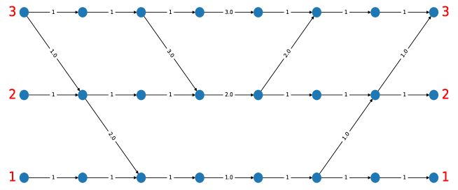
Figure 2: Planar network associated with the I-TN matrix $A$ in (5).

We note in passing that, conversely, any planar network can be associated with a TN matrix [16]. This association is unique in case of an I-TN matrix.

Remark 2.

Since the planar network of any I-TN matrix is associated with an SEB factorization, it admits a special structure. First, all horizontal edges have positive weights, where horizontal edges corresponding to the matrix $D$ (in the center of the network) have weight $d_{i}$, $i=1,\dots,n$, and all other horizontal edges have weight one. In addition, the left-hand side [right-hand side] of the network, corresponding to the product of all $L_{i}$ [$U_{i}$] matrices, consists of only downward [upward] pointing diagonal edges. This structure holds for all I-TN matrices. Only the weights of the diagonal edges and the horizontal edges corresponding to the matrix $D$ differ among different I-TN matrices.

The following important result associates the minors of $A$ to its planar network. Its proof follows from the Cauchy-Binet formula.

Proposition 6.

[9, Ch. 2] Let $A:=A_{1}\cdots A_{p}$, where each $A_{i}$ is either an EB matrix ($L$ or $U$) or a diagonal matrix with positive diagonal entries. Recall that the network associated with $A$ is obtained by concatenating left to right the diagrams associated with $A_{1},\dots,A_{p}$, respectively. Then $A(\{i_{1},\dots,i_{k}\}|\{j_{1},\dots,j_{k}\})$ is equal to the weight of the set of vertex-disjoint families in the network connecting the sources $\{i_{1},\dots,i_{k}\}$ to the sinks $\{j_{1},\dots,j_{k}\}$. In particular, $a_{ij}=A(\{i\}|\{j\})$ is equal to the sum of all the weights of paths that join source $i$ to sink $j$.

The next example demonstrates Proposition 6.

Example 3.

Let

$$A=\begin{bmatrix}3&1&0&0\\ 1&4&1&0.1\\ 0.1&1&5&3\\ 0&0&2&7\end{bmatrix}.$$ (8)

It is straightforward to verify that $A$ is I-TN. The associated network of $A$ is depicted in Figure 3 (all numerical values in this paper are to four-digit accuracy).

There is only one directed path joining the source $2$ with the sink $4$, and the weight of this path is $3.6667\cdot 0.2727\cdot 0.1\approx 0.1$. Indeed, $a_{2,4}=0.1$.

There are two paths that join source $2$ with sink $2$: the horizontal path with weight $3.6667$, and the path with weight $0.3333\cdot 3\cdot 0.3333\approx 0.3333$. The sum of these two path weights is $4$, and this is equal to $a_{22}$.

As another example, consider $A(\{1,3\}|\{2,3\})$. In this case, there are three families of vertex-disjoint paths joining the sources $\{1,3\}$ with the sinks $\{2,3\}$:

1. The path joining source $1$ with sink $2$ with weight $3\cdot 0.3333\approx 1$, and the path joining source $3$ with sink $3$ with weight $4.7364$. This family weight is then $1\cdot 4.7364=4.7364$.

2. The path joining source $1$ with sink $2$ with weight $3\cdot 0.3333\approx 1$, and the path joining source $3$ with sink $3$ with weight $0.1\cdot 3.6667\cdot 0.2727\approx 0.1$. This family weight is then $1\cdot 0.1=0.1$.

3. The path joining source $1$ with sink $2$ with weight $3\cdot 0.3333\approx 1$, and the path joining source $3$ with sink $3$ with weight $0.1636\cdot 3.6667\cdot 0.2727\approx 0.1636$. This family weight is then $1\cdot 0.1636=0.1636$.

The sum over these three families is $4.7364+0.1+0.1636=5$, and $A(\{1,3\}|\{2,3\})=\det(\begin{bmatrix}1&0\\ 1&5\end{bmatrix})=5$.

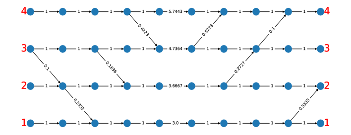
Figure 3: Planar network associated with $A$ in (8).

Proposition 6 links the minors of an I-TN matrix to the topology of the associated planar network. This has many theoretical and practical implications. For example, the following known proposition follows immediately from Proposition 6, as horizontal edges with positive weights always exist in the planar network of any I-TN matrix (see Remark 2).

Proposition 7.

[19, Ch. 1] Let $A\in\mathbb{R}^{n\times n}$ be an I-TN matrix. Then every principal minor of $A$ is positive.

Proposition 6 is one of the main tools we use to derive the results below.

3 Main Results

Since an oscillatory matrix $A$ is in particular TN, Proposition 3 implies that verifying that $A^{k}$ is TP is equivalent to verifying that all the corner minors of $A^{k}$ are positive. The next result shows that when $A$ is the product of matrices that appear in the SEB factorization it is possible in some sense to “decouple” the examination of lower-left corner and upper-right corner minors. We say that a diagonal matrix $D\in\mathbb{R}^{n\times n}$ is positive if all its diagonal entries are positive.

Proposition 8.

Let $A:=A_{1}\cdots A_{p}$, where each $A_{j}\in\mathbb{R}^{n\times n}$ is either an EB matrix ($L_{i}$ or $U_{i}$) or a positive diagonal matrix. Pick $c\in\{1,\dots,n-1\}$, and let $\alpha:=\{n-c+1,\dots,n\}$, $\beta:=\{1,\dots,c\}$, so that $A(\alpha|\beta)$ is a lower-left corner minor of $A$. Let $w=w(A,c)$ be the minimal integer such that in the planar network associated with $A^{w}$ there is a path connecting $x$ to $x-n+c$ for any $x\in\alpha$. Then $w$ does not change if we replace every $U_{i}$ in $A$ with any positive diagonal matrix.

In other words, the non-horizontal edges in the planar network corresponding to the $U_{i}$s do not affect $w$.

By transposition, this implies a similar result for any upper-right corner minor $A(\beta|\alpha)$, namely, the minimum number of copies $v$ of $A$ needed to guarantee the existence of a path connecting $y$ to $y+n-c$ for any $y\in\beta$ does not depend on the non-horizontal edges in the $L_{i}$s.

We now describe another implication of Proposition 8. Let $A=L_{a}D_{a}U_{a}$, $B=L_{b}D_{b}U_{b}$ be I-TN such that $L_{a}$ and $L_{b}$ [$U_{a}$ and $U_{b}$] denote the product of all the $L_{i}$ [$U_{i}$] matrices in the SEB factorization of $A$ and $B$. Suppose that a parameter in the bidiagonal factorization of $L_{a}$ is positive if and only if (iff) the corresponding parameter in the bidiagonal factorization of $L_{b}$ is positive. Then a lower-left corner minor of $A$ is positive iff the same minor in $B$ is positive.

Proof of Proposition 8. If $w(A,c)$ is infinite then clearly it will remain infinite if we replace every $U_{i}$ in $A$ with some positive diagonal matrix. So we may assume that $w(A,c)$ is finite.

Let $G^{w}$ denote the network corresponding to $w$ concatenated copies of the network of $A$. Then $w(A,c)>0$ iff $G^{w}$ includes a family of vertex disjoint paths that include: a path $P_{c}$ from $n$ to $c$; a path $P_{c-1}$ from $n-1$ to $c-1$; $\dots$; and a path $P_{1}$ from $n-c+1$ to $1$. If none of these $P_{i}$s includes an upward pointing diagonal edge from some $U_{s}$ then we are done. Otherwise, there exists a minimal $i$ such that $P_{i}$ includes an upward pointing diagonal edge from some $U_{s}$. This edge points from a node $v_{r}$ to a node $v_{r+1}$ for some $r\in\{1,\dots,n-1\}$. The continuation of $P_{i}$ after this edge must include a downward pointing diagonal edge from a node $v_{r+1}$ to $v_{r}$. Let $\tilde{P}_{i}$ be the path obtained from $P_{i}$ by replacing this part in $P_{i}$ by a set of horizontal arcs connecting $v_{r}$ to $v_{r}$. Then $\{P_{c},P_{c-1},\dots,P_{i+1},\tilde{P}_{i},P_{i-1},\dots,P_{1}\}$ is a set of vertex disjoint paths that connect every $x\in\alpha$ to $(x-n+c)\in\beta$ using the same number of copies of $A$. Thus, we may assume that $P_{i}$ does not include any upward pointing diagonal edges. Now we can apply the same idea to any upward pointing diagonal edge in $P_{i+1}$ and so on.  $\square$

To proceed, we introduce a notation that simplifies the representation of the factorization in (1). For $i\in\{2,\dots,n\}$, define:

$$x_{i}:=1+(i-2)n-\sum_{j=1}^{i-2}j=(i-2)n-\frac{(i-3)i}{2},$$

and

$$\ell^{i}:=\begin{bmatrix}\ell_{x_{i}}&\cdots&\ell_{x_{i}+n-i}\end{bmatrix}^{T},\text{ and }u^{i}:=\begin{bmatrix}u_{x_{i}}&\cdots&u_{x_{i}+n-i}\end{bmatrix}^{T}.$$ (9)

Thus,

$$\ell^{2} =\begin{bmatrix}\ell_{1}&\cdots&\ell_{n-1}\end{bmatrix}^{T}\in\mathbb{R}_{+}^{n-1},$$

$$\ell^{3} =\begin{bmatrix}\ell_{n}&\cdots&\ell_{2n-3}\end{bmatrix}^{T}\in\mathbb{R}_{+}^{n-2},$$

$$\vdots$$

$$\ell^{n} =\ell_{k}\in\mathbb{R}_{+},$$

and similarly for $u^{i}$. Let $\ell^{i}_{j}$ [$u^{i}_{j}$] denote the $j$’th entry in $\ell^{i}$ [$u^{i}$], and let

$$W_{i}(\ell^{i}) :=\prod_{j=n}^{i}L_{j}(\ell^{i}_{n-j+1}),$$

$$Q_{i}(u^{i}) :=\prod_{j=i}^{n}U_{j}(u^{i}_{j-i+1}).$$ (10)

Then the SEB factorization (1) can be written more succinctly as

$$A=W_{2}(\ell^{2})\cdots W_{n}(\ell^{n})DQ_{n}(u^{n})\cdots Q_{2}(u^{2}).$$ (11)

For $A\in\mathbb{R}^{n\times n}$, let $r_{\ell}(A)$ denote the minimal integer $w>0$ such that all the lower-left corner minors of $A^{w}$, except perhaps for $\det(A)$, are positive. Similarly, let $r_{u}(A)$ denote the minimal integer $v>0$ such that all the upper-right corner minors of $A^{v}$, except perhaps for $\det(A)$, are positive.

Theorem 2.

Let $A\in\mathbb{R}^{n\times n}$ be oscillatory, and write its SEB factorization as in (11). Then

$$r(A)=\max\left\{r_{\ell}\left(W_{2}(\ell^{2})\dots W_{n}(\ell^{n})\right),r_{u}\left(Q_{n}(u^{n})\dots Q_{2}(u^{2})\right)\right\}.$$

Proof of Theorem 2. Since $A$ is oscillatory, it is TN and $\det(A)>0$. Hence, $r(A)=\max\left\{r_{\ell}\left(A\right),r_{u}\left(A\right)\right\}$. Combining this with the fact that every $W_{i}$ [$Q_{i}$] is a product of $L_{j}$s [$U_{j}$s] and Proposition 8 completes the proof.  $\square$

Theorem 2 can be applied to determine $r(A)$ explicitly for large classes of oscillatory matrices. Indeed, suppose that for some specific structure of $W_{2}(\ell^{2})\cdots W_{n}(\ell^{n})$, denoted $W$, we can explicitly determine $r_{\ell}\left(W\right)$. A typical case is when there exists a “worst-case” lower-left corner minor $(\alpha|\beta)$, that is, if $W^{k}(\alpha|\beta)>0$ for some $k>0$ then all lower-left corner minors of $W^{k}$ (except perhaps for $\det(W^{k})$) are positive. If it is possible to determine the minimal $j$ such that $W^{j}(\alpha|\beta)>0$ then $r_{\ell}\left(W\right)=j$.

By transposition, we also know $r_{u}(W^{T})$. Thus, we know $r(A)$ for $A=WDW^{T}$, for any positive diagonal matrix $D$. To demonstrate these ideas, we now define two classes of $n\times n$ matrices, denoted $Z_{i}(s)$, $i=1,2$. Each class includes matrices parametrized by a non-negative integer $s$, taking values in a domain $D_{i}$, $i=1,2$. In the definitions of these classes below it is always assumed that all the multipliers are positive.

Definition 2.

$Z_{1}(s)$, $s\in D_{1}:=\{2,\dots,n\}$, is the class of matrices in the form:

$$W_{2}(\ell^{2})\cdots W_{s}(\ell^{s}),$$

where all the multipliers are positive.

The planar network of $Z_{1}(s)$ is the product of the networks for $W_{2}(\ell^{2})$, $\dots$, $W_{s}(\ell^{s})$. This includes horizontal lines, and $s-1$ downward pointing diagonal lines: the first from $n$ to $1$, the second from $n$ to $2$, and so on. Figure 4 depicts this network for $n=6$ and $s\in\{2,\dots,6\}$.

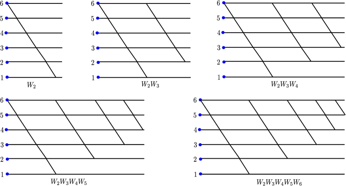
Figure 4: Planar network corresponding to $Z_{1}(s)$ for $n=6$ and $s\in\{2,\dots,6\}$. Upper-left figure corresponds to $s=2$, upper-middle to $s=3$, upper-right to $s=4$, lower-left to $s=5$, and lower-right to $s=6$.

For $y\in\mathbb{R}$, let $\lceil y\rceil$ denote the smallest integer that is larger than or equal to $y$.

Proposition 9.

Pick $s\in D_{1}$ and a matrix $A\in Z_{1}(s)$. Let $\mu_{1}:=\left\lceil\frac{n-1}{s-1}\right\rceil$. Then $r_{\ell}(A)=\mu_{1}$.

Proof of Proposition 9. Let $\alpha:=\{2,3,\dots,n\}$ and $\beta:=\{1,2,\dots n-1\}$. Suppose that $A^{w}(\alpha|\beta)>0$ for some $w>0$. Since each copy of $A$ contains $s-1$ diagonal lines corresponding to $W_{2}(\ell^{2})\cdots W_{s}(\ell^{s})$ (see Figure 4), the $n-1$ vertex-disjoint paths corresponding to $A^{w}(\alpha|\beta)$ require at least $\mu_{1}$ copies of $A$. We conclude that

$$r_{\ell}(A)\geq\mu_{1}.$$ (12)

We now show that $A^{\mu_{1}}(\alpha|\beta)>0$. We introduce more notation. Consider the network corresponding to $A^{\mu_{1}}$. The symbol $\searrow$ represents a diagonal arc from one of $W_{2}(\ell^{2}),\dots,W_{s}(\ell^{s})$ in some copy of $A$, and is accompanied by an explanation of which $L_{j}$ is used. We now describe a set of paths in the network corresponding to $A^{\mu_{1}}$. The first path is

$$P_{2}:\;2 \to 2\to\dots\to 2\searrow 1\to 1\to\dots\to 1,$$

where $\searrow$ is from $L_{2}$ in the first copy of $W_{2}$. The second path is

$$P_{3}:\;3 \to 3\to\dots\to 3\searrow 2\to 2\to\dots\to 2,$$

where $\searrow$ is from $L_{3}$ in the first copy of $W_{3}$ if $s>2$ or from $L_{3}$ in the second copy of $W_{2}$ if $s=2$. Note that this implies that $P_{2}$ and $P_{3}$ are vertex-disjoint. The last path is

$$P_{n}:\;n \to n\to\dots\to n\searrow n-1\to n-1\to\dots\to n-1,$$

where $\searrow$ is from $L_{n}$ in the first possible copy of some $W_{i}$ such that $P_{n}$ and $P_{n-1}$ are vertex-disjoint. Note that all these paths are vertex-disjoint by construction.

The paths $P_{2},\dots,P_{s}$ use the first copy of $W_{2}(\ell^{2})\cdots W_{s}(\ell^{s})$. The paths $P_{s+1},\dots,P_{2s-1}$ use the second copy of $W_{2}(\ell^{2})\cdots W_{s}(\ell^{s})$, and so on. This implies that $\mu_{1}$ copies of $A$ are indeed enough to realize this family of $n-1$ vertex-disjoint paths, so $A^{\mu_{1}}(\alpha|\beta)>0$.

Pick $c\in\{1,\dots,n-2\}$. Let $\gamma:=\{n-c+1,\dots,n\}$ and $\delta:=\{1,\dots,c\}$. Then $A(\gamma|\delta)$ is a lower-left corner minor, $(\gamma|\delta)\not=(\alpha|\beta)$, and $A(\gamma|\delta)$ is not the determinant of $A$. To complete the proof, we need to show that $A^{\mu_{1}}(\gamma|\delta)>0$. To do this, we generate a set of vertex-disjoint paths connecting every $x\in\gamma$ to $(x-n+c)\in\delta$. We do this by modifying the paths $P_{i}$ described above. First, delete the paths $P_{n},\dots,P_{c+2}$, as these are not needed now. The path $P_{c+1}$ contains an arc connecting vertex $c+1$ to $c$. The structure of the diagonal lines in the network (see Figure 4) implies that we can extend this arc to a path $\tilde{P}_{c+1}$ connecting $n$ to $c$, as every diagonal line emanates from $n$. The path $P_{c}$ contains an arc connecting vertex $c$ to $c-1$. This path can be extended similarly to a path $\tilde{P}_{c}$ connecting $n-1$ to $c-1$ that does not intersect nor touch $\tilde{P}_{c+1}$. Continuing in this fashion shows that $A^{\mu_{1}}(\gamma|\delta)>0$.  $\square$

The second class of parametrized matrices, denoted $Z_{2}(s)$, requires more notation. Note that the multiplier of $L_{i}$ in $W_{i}(\ell^{i})$ is $\ell^{i}_{n-i+1}=\ell_{x_{i}+n-i}$. For any $i=2,\dots,n-1$, we define a subset of $W_{i}(\ell^{i})$ by

$$\Psi_{i}(\ell^{i}):=\{W_{i}(\ell^{i}):\ell_{x_{i}+n-i}>0,\;\prod_{j=x_{i}}^{x_{i}+n-i-1}\ell_{j}=0\}.$$ (13)

This describes all the cases where the multiplier of $L_{i}$ is positive, and at least one of the other multipliers is zero. For example, for $n=5$,

$$\Psi_{2}(\ell^{2}) =\{L_{2},L_{3}L_{2},L_{4}L_{2},L_{5}L_{2},L_{4}L_{3}L_{2},L_{5}L_{4}L_{2},L_{5}L_{3}L_{2}\},$$

$$\Psi_{3}(\ell^{3}) =\{L_{3},L_{4}L_{3},L_{5}L_{3}\},$$

$$\Psi_{4}(\ell^{4}) =\{L_{4}\},$$

where it is understood that all the multipliers are positive.

Definition 3.

$Z_{2}(s)$, $s\in D_{2}:=\{2,\dots,n\}$, is the class of matrices in the form:

$$L_{2}(\ell_{2})\cdots L_{s-2}(\ell_{s-2})P(\ell^{s-1})W_{s}(\ell^{s})\cdots W_{n}(\ell^{n}),$$ (14)

where $P(\ell^{s-1})\in\Psi_{s-1}(\ell^{s-1})$, and all the multipliers are positive.

Thus, $Z_{2}$ includes all the matrices in the form

$$W_{2}W_{3}\dots W_{n},$$

$${P_{2}}W_{3}\cdots W_{n},$$

$$L_{2}P_{3}W_{4}\cdots W_{n},$$

$$\vdots$$

$$L_{2}\cdots L_{n-2}P_{n-1}W_{n},$$

where $P_{i}\in\Psi_{i}$.

A special case is when $P(\ell^{s-1})=L_{s-1}(\ell^{s-1})$ and then (14) becomes

$$L_{2}(\ell_{2})\cdots L_{s-2}(\ell_{s-2})L_{s-1}(\ell_{s-1})W_{s}(\ell^{s})\cdots W_{n}(\ell^{n}).$$

The planar network associated with $Z_{2}(s)$ represents the product $L_{2}\cdots L_{s-2}PW_{s}\cdots W_{n},$ with $P\in\Psi_{s-1}$ (we omit the parameters for the sake of clarity). Note that $P$ must include the matrix $L_{s-1}$, and must not include at least one of the matrices $L_{n},\dots,L_{s}$. This network includes horizontal lines, and at least $n-1$ downward pointing diagonal lines. There are $n-s+1$ diagonal lines corresponding to $W_{x}$, $x=s,\dots,n$. Each such line connects $n$ to $x-1$. There are another $s-3$ diagonal lines corresponding to $L_{x}$, $x=2,\dots,s-2$. Each such line connects $x$ to $x-1$. The matrix $P$ corresponds to a diagonal arc that connects $s-1$ to $s-2$, and may also include other diagonal arcs. Figure 5 depicts this network for $n=6$, the particular case $P=L_{s-1}$, and all $s\in\{2,\dots,6\}$.

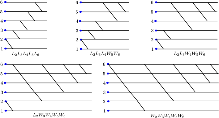
Figure 5: Planar network corresponding to $Z_{2}(s)$ with $n=6$, the particular case $P=L_{s-1}$, and $s\in\{2,\dots,6\}$. Upper-left figure corresponds to $s=6$, upper-middle to $s=5$, upper-right to $s=4$, lower-left to $s=3$, and lower-right to $s=2$.

Proposition 10.

Pick $s\in D_{2}$ and a matrix $A\in Z_{2}(s)$. Let $\mu_{2}:=s-1$. Then $r_{\ell}(A)=\mu_{2}$.

Proof of Proposition 10. We first assume that $P=L_{n-1}$. Let $\alpha:=\{n\}$ and $\beta:=\{1\}$. We claim that

$$\min\{k:A^{k}(\alpha|\beta)>0\}=\mu_{2}.$$ (15)

Indeed, in the network of (every copy) of $A$ the longest downward pointing diagonal connects $n$ to $s-1$. For any vertex in $\{s-2,s-3,\dots,1\}$ (i.e. all the vertices “below” $s-1$) the longest downward pointing diagonal is a single arc. This implies that at least $n-(n-s+1)=\mu_{2}$ copies of $A$ are needed to realize a path from the source vertex $n$ to the sink vertex $1$. Given this number of copies, the path is:

$$n\searrow s-1\searrow s-2\searrow s-3\searrow\cdots\searrow 1.$$

This proves (15).

Pick $c\in\{2,\dots,n-1\}$. Let $\gamma:=\{n-c+1,\dots,n\}$ and $\delta:=\{1,\dots,c\}$. Then $(\gamma|\delta)$ is a lower-left corner minor that is not $(\alpha|\beta)$ nor the determinant of $A$. To complete the proof, we need to show that $A^{\mu_{2}}(\gamma|\delta)>0$. To do this, we generate a set of vertex-disjoint paths connecting every $x\in\gamma$ to $(x-n+c)\in\delta$ in the network of $A^{\mu_{2}}$: in the first copy, we use

$$n-c+1\searrow s-1,$$

$$n-c+2\searrow s,$$

$$\;\vdots$$

$$n\searrow c+s-2.$$

Note that this is vertex-disjoint set of paths. In the second copy, we use

$$s-1\searrow s-2,$$

$$s\searrow s-1,$$

$$\;\vdots$$

$$c+s-2\searrow c+s-3.$$

and similar “one-step” paths in all the next copies. Then $\mu_{2}=s-1$ copies are always enough for a set of vertex-disjoint paths connecting every $x\in\gamma$ to $(x-n+c)\in\delta$, and this completes the proof when $P=L_{n-1}$.

Now assume that $P\neq L_{s-1}$, i.e. $P=QL_{s-1}$, where $Q$ contains at least one matrix from $L_{n},\dots,L_{s}$, but not all of these matrices. In the planar network of $Q$ the longest possible downward pointing diagonal that starts from the vertex $n$ contains $n-s$ consecutive edges, corresponding to $Q=L_{n}\cdots L_{s+1}$. Since the downward pointing diagonal line corresponding to $W_{s}$ starts from $n$ and contains $n-s+1$ consecutive edges, using diagonal lines corresponding to $Q$ cannot reduce the number of copies of $A$ required to obtain a path from the source vertex $n$ to the sink vertex $1$. This completes the proof.  $\square$.

The next result follows from Theorem 2 and Propositions 9 and 10.

Corollary 1.

Let $A\in\mathbb{R}^{n\times n}$ be an oscillatory matrix. If $A=LDU$ with $L\in Z_{i}(s_{i})$ for some $i\in\{1,2\}$, $D$ a positive diagonal matrix, and $U^{T}\in Z_{j}(s_{j})$ for some $j\in\{1,2\}$, then

$$r(A)=\max\{\mu_{i}(s_{i}),\mu_{j}(s_{j})\}.$$ (16)

Note that $\mu_{1}(s)$ takes values in $\{n-1,\left\lceil\frac{n-1}{2}\right\rceil,\left\lceil\frac{n-1}{3}\right\rceil,\dots,1\}$, and $\mu_{2}(s)$ takes values in $\{1,2,\dots,n-1\}$, so Corollary 1 covers oscillatory matrices with all possible exponent values.

The following examples demonstrate our theoretical results.

Example 4.

Suppose that $L\in Z_{1}(n)$ and $U^{T}\in Z_{1}(n)$. In this case, all the multipliers in the SEB factorization of $A=LDU$ are positive, so Proposition 4 implies that $A$ is TP. On the other-hand, (16) gives

$$r(A)=\max\{\mu_{1}(n),\mu_{1}(n)\}=\lceil\frac{n-1}{n-1}\rceil=1.$$

As another example, suppose that $L\in Z_{1}(2)$ and $U^{T}\in Z_{1}(2)$. Then $A$ is as in (7), and (16) gives

$$r(A)=\max\{\mu_{1}(2),\mu_{1}(2)\}=\lceil\frac{n-1}{1}\rceil=n-1.$$

This recovers one of the results in [7].

For a vector $x=\begin{bmatrix}x_{1}&x_{2}&\dots&x_{n}\end{bmatrix}^{T}\in\mathbb{R}^{n}$, let $\underline{x}:=\begin{bmatrix}x_{n}&x_{n-1}&\dots&x_{1}\end{bmatrix}^{T}$.

Example 5.

As a more concrete example, consider

$$A=\begin{bmatrix}1&1&2&2\\ 2&3&7&9\\ 6&9&22&30\\ 6&9&22&31\end{bmatrix},$$

which is I-TN, but not TP (for example, $A(\{2,3\}|\{1,2\})=0$). The SEB factorization of $A$ is

$$A =L_{4}(1)L_{3}(3)L_{2}(2)IU_{3}(1)U_{4}(2)U_{2}(1)U_{3}(2)U_{4}(1)$$

$$=W_{2}(\ell^{2})Q_{3}(u^{3})Q_{2}(u^{2}),$$

with $\ell^{2}=\begin{bmatrix}1&3&2\end{bmatrix}^{T}$, $u^{3}=\begin{bmatrix}1&2\end{bmatrix}^{T}$, and $u^{2}=\begin{bmatrix}1&2&1\end{bmatrix}^{T}$, i.e. $A$ is oscillatory. Since $L=W_{2}(\ell^{2})\in Z_{1}(2)$ and $U^{T}=W_{2}(\underline{u^{2}})W_{3}(\underline{u^{3}})\in Z_{1}(3)$,

$$r(A)=\max\{\mu_{1}(2),\mu_{1}(3)\}=\max\{3,2\}=3.$$

Indeed,

$$A^{2}=\begin{bmatrix}27&40&97&133\\ 104&155&377&520\\ 336&501&1219&1683\\ 342&510&1241&1714\end{bmatrix},$$

and so $(A^{2})(\{2,3,4\}|\{1,2,3\})=0$, thus $A^{2}$ is not TP, implying that indeed $r(A)=3$.

Example 6.

Let $L\in Z_{2}(2)$ and $U^{T}\in Z_{2}(2)$. This also means that $L\in Z_{1}(n)$ and $U^{T}\in Z_{1}(n)$, and by Example 4, $r(A)=1$. Indeed Eq. (16) gives

$$r(A)=\max\{\mu_{2}(2),\mu_{2}(2)\}=1.$$

Now assume that $L\in Z_{2}(n)$ and $U^{T}\in Z_{2}(n)$. Thus, $A$ is as in (6) (note that $W_{n}(\ell^{n})=L_{n}(\ell_{k})$ and $Q_{n}(u^{n})=U_{n}(u_{k})$), and in this case

$$r(A)=\max\{\mu_{2}(n),\mu_{2}(n)\}=n-1$$

(see [7]).

As a concrete example, consider

$$A=\begin{bmatrix}1&2&0&0&0\\ 2&5&3&0&0\\ 0&2&7&2&6\\ 0&8&29&11&34\\ 0&24&89&41&131\end{bmatrix},$$

which is I-TN, but clearly not TP. The SEB factorization of $A$ is

$$A =L_{2}(2)L_{5}(3)L_{4}(4)L_{3}(2)L_{5}(2)L_{4}(1)L_{5}(2)IU_{5}(1)U_{4}(2)U_{5}(3)U_{3}(3)U_{2}(2)$$

$$=L_{2}(2)W_{3}(\ell^{3})W_{4}(\ell^{4})W_{5}(\ell^{5})Q_{5}(u^{5})Q_{4}(u^{4})U_{3}(3)U_{2}(2),$$

with $\ell^{3}=\begin{bmatrix}3&4&2\end{bmatrix}^{T}$, $\ell^{4}=\begin{bmatrix}2&1\end{bmatrix}^{T}$, $\ell^{5}=2$, $u^{5}=1$, and $u^{4}=\begin{bmatrix}2&3\end{bmatrix}^{T}$, i.e. $A$ is oscillatory. Since $L=L_{2}(2)W_{3}(\ell^{3})W_{4}(\ell^{4})W_{5}(\ell^{5})\in Z_{2}(3)$ and $U^{T}=L_{2}(2)L_{3}(3)W_{4}(\underline{u^{4}})W_{5}(\underline{u^{5}})\in Z_{2}(4)$,

$$r(A)=\max\{\mu_{2}(3),\mu_{2}(4)\}=\max\{2,3\}=3.$$

Since $A^{2}(1,4)=0$, $A^{2}$ is not TP. It can be verified that $A^{3}$ is TP, implying that indeed $r(A)=3$.

We now describe several generalizations of our results.

3.1 Generalizations

In many SEB factorizations of oscillatory matrices, $L$ or $U^{T}$ can be rewritten as a class in $Z_{1}$ or $Z_{2}$. We demonstrate this using an example. Consider the case $n=5$ and the product

$$U:=[U_{5}(u_{1})][U_{4}(u_{2})U_{5}(u_{3})][U_{3}(u_{4})U_{4}(u_{5})U_{5}(u_{6})][U_{2}(u_{7})U_{3}(u_{8})U_{4}(u_{9})U_{5}(u_{10})],$$

with $u_{3}=u_{5}=u_{8}=u_{10}=0$, and all the other multipliers positive, that is,

$$U=U_{5}(u_{1})U_{4}(u_{2})U_{3}(u_{4})U_{5}(u_{6})U_{2}(u_{7})U_{4}(u_{9}).$$

This seems to suggest that $U^{T}\notin(Z_{1}\cup Z_{2})$. However, using (2.1) yields

$$U =U_{5}(u_{1})U_{4}(u_{2})U_{5}(u_{6})U_{3}(u_{4})U_{4}(u_{9})U_{2}(u_{7})$$

$$=Q_{5}(u^{5})Q_{4}(u^{4})U_{3}(u_{4})U_{4}(u_{9})U_{2}(u_{7}),$$

with

$$u^{5}:=u_{1},\;u^{4}:=\begin{bmatrix}u_{2}&u_{6}\end{bmatrix}^{T}.$$

Thus, $U^{T}\in Z_{2}(4)$ (with $P=L_{4}(u_{9})L_{3}(u_{4})$).

This suggests that in many factorizations, $L$ and $U^{T}$ can be rewritten as classes in $Z_{1}\cup Z_{2}$, and thus the corresponding exponent can be determined explicitly.

Our analysis uses the fact that certain edges in the associated planar networks have positive weights, while ignoring their actual value. Thus, another generalization is to arbitrary products of oscillatory matrices.

Corollary 2.

Consider a set of matrices $\{A_{x}\}_{x=1}^{m}$, where every $A_{x}\in\mathbb{R}^{n\times n}$ is oscillatory. Let $L(x)$ [$U(x)$] denotes the product of all $L_{i}$ [$U_{i}$] matrices in the SEB factorization of $A_{x}$. Suppose that there exist $i,j,s_{i},s_{j}$ such that $L(x)\in Z_{i}(s_{i})$ and $(U(x))^{T}\in Z_{j}(s_{j})$ for all $x$, but possibly every $L(x)$ and every $U(x)$ has a different set of multiplier values. Then a product of any $k$ matrices from the set is TP iff

$$k\geq\max\{\mu_{i}(s_{i}),\mu_{j}(s_{j})\}.$$

The next example demonstrates this.

Example 7.

Let

$$A_{1}=\begin{bmatrix}2&8&16&48\\ 8&33&67&203\\ 8&39.5&89.5&289.5\\ 20&134.5&350.5&1219.5\end{bmatrix},\quad A_{2}=\begin{bmatrix}1&2&8&24\\ 2&6&28&88\\ 6&23&117&376\\ 30&145&789&2580\end{bmatrix}.$$

The SEB factorizations are:

$$A_{1} =L_{4}(2.5)L_{3}(1)L_{2}(4)L_{4}(5.5)L_{3}(6.5)L_{4}(1)D_{1}U_{3}(1)U_{4}(2)U_{2}(4)U_{3}(2)U_{4}(3),$$

$$A_{2} =L_{4}(5)L_{3}(3)L_{2}(2)L_{4}(6)L_{3}(2.5)L_{4}(2)D_{2}U_{3}(2)U_{4}(1)U_{2}(2)U_{3}(4)U_{4}(3),$$

with $D_{1}:=\operatorname{diag}(2,1,3,5)$ and $D_{2}:=\operatorname{diag}(1,2,3,4)$. This implies that $A_{1}$ and $A_{2}$ are oscillatory matrices, but not TP (see Propositions 4 and 5). Note that,

$$L(1) =L_{4}(2.5)L_{3}(1)L_{2}(4)L_{4}(5.5)L_{3}(6.5)L_{4}(1),$$

$$L(2) =L_{4}(5)L_{3}(3)L_{2}(2)L_{4}(6)L_{3}(2.5)L_{4}(2),$$

$$U(1) =U_{3}(1)U_{4}(2)U_{2}(4)U_{3}(2)U_{4}(3),$$

$$U(2) =U_{3}(2)U_{4}(1)U_{2}(2)U_{3}(4)U_{4}(3).$$

This implies that both $L(1)$ and $L(2)$ [$(U(1))^{T}$ and $(U(2))^{T}$] belong to $Z_{1}(4)$ [$Z_{1}(3)$], where each has a different set of parameter values. Thus,

$$r(A_{1})=r(A_{2})=\max\{\mu_{1}(4),\mu_{1}(3)\}=\max\{1,2\}=2.$$

It is straightforward to verify that indeed $A_{1}^{2}$, $A_{2}^{2}$, $A_{1}A_{2}$, and $A_{2}A_{1}$ are all TP matrices. Note that since $\mu_{1}(4)=1$, our theoretical results show that all the lower-left corner minors (except perhaps for the determinant) of both $A_{1}$ and $A_{2}$ are positive.

Note that in general given a set $\{A_{x}\}_{x=1}^{m}$ of oscillatory matrices, with $r(A_{x})=w$ for all $x=1,\dots,m$, it is possible that a product of less than $w$ matrices from the set is TP. This is demonstrated in the following example.

Example 8.

Consider the matrices

$$A_{1}=\begin{bmatrix}1&1&2&6\\ 3&4&9&28\\ 3&4&10&32\\ 6&8&20&65\end{bmatrix},\quad A_{2}=\begin{bmatrix}1&3&3&6\\ 2&7&7&14\\ 6&23&24&48\\ 6&25&27&55\end{bmatrix}.$$

Their factorizations are

$$A_{1} =L_{4}(2)L_{3}(1)L_{2}(3)U_{3}(1)U_{4}(1)U_{2}(1)U_{3}(2)U_{4}(3),$$

$$A_{2} =L_{4}(1)L_{3}(3)L_{2}(2)L_{4}(1)L_{3}(2)U_{2}(3)U_{3}(1)U_{4}(2).$$

Thus, $L(1)\in Z_{1}(2)$, $(U(1))^{T}\in Z_{1}(3)$, $L(2)\in Z_{1}(3)$, and $(U(2))^{T}\in Z_{1}(2)$.Thus,

$$r(A_{1})=\max\{\left\lceil\frac{4-1}{2-1}\right\rceil,\left\lceil\frac{4-1}{3-1}\right\rceil\}=3,$$

and

$$r(A_{2})=\max\{\left\lceil\frac{4-1}{3-1}\right\rceil,\left\lceil\frac{4-1}{2-1}\right\rceil\}=3.$$

However, it can be verified that both $A_{1}A_{2}$ and $A_{2}A_{1}$ are TP, i.e. we do not necessarily need a product of three matrices to obtain a TP matrix.

3.2 Upper-Bounds on $r(A)$

It is clear that adding new edges to a planar network associated with an oscillatory matrix can never increase its exponent value. Thus, if a given class of oscillatory matrices can be factored as matrices in $Z_{i}$ multiplied by additional terms, then our results can be used to derive an upper bound on their exponent. This is stated formally in the next result.

Corollary 3.

Let $A=LDU\in\mathbb{R}^{n\times n}$ be an oscillatory matrix. If there exist $i,j$ such that either $L\in Z_{i}(s_{i})$ and $U^{T}$ belongs to $Z_{j}(s_{j})$ multiplied by some additional terms, or $U^{T}\in Z_{j}(s_{j})$ and $L$ belongs to $Z_{i}(s_{i})$ multiplied by some additional terms, then

$$r(A)\leq\max\{\mu_{i}(s_{i}),\mu_{j}(s_{j})\}.$$

For example, suppose that $A\in\mathbb{R}^{5\times 5}$ can be factored as

$$A=L_{3}(\ell_{3})L_{2}(\ell_{4})L_{3}(\ell_{7})W_{4}(\ell^{4})W_{5}(\ell^{5})DQ_{5}(u^{5})Q_{4}(u^{4})U_{3}(u_{7})U_{2}(u_{4}).$$

Then $L=L_{3}(\ell_{3})W$, where $W:=L_{2}(\ell_{4})L_{3}(\ell_{7})W_{4}(\ell^{4})W_{5}(\ell^{5})$, and $U^{T}\in L_{2}(u_{4})L_{3}(u_{7})W_{4}(u^{4})W_{5}(u^{5})$. Here $U^{T}\in Z_{2}(4)$, and since $W\in Z_{2}(4)$, we see that $L$ belongs to $Z_{2}(4)$ multiplied by the additional term $L_{3}(\ell_{3})$. Thus, $r(A)\leq\mu_{2}(4)=3$.

The mapping from the SEB factorization of $A$ to $r(A)$ is nontrivial. There are known cases where adding specific additional terms necessarily reduces the exponent [7]. But in general adding terms with positive multipliers to $L\in Z$ or to $U^{T}\in Z$ does not necessarily decrease $r(A)$ and thus in these cases the bound in Corollary 3 may be tight. For example, if $r(A)=2$ then adding terms to the SEB factorization of $A$ cannot decrease $r(A)$ unless the modified factorization includes all the multipliers in (1), as the SEB factorization of a TP matrix is unique. The following example demonstrates this.

Example 9.

Let

$$A=\begin{bmatrix}1&1&4\\ 1&2&10\\ 0&2&13\end{bmatrix}.$$

Its SEB factorization is $L_{2}(1)L_{3}(2)IU_{3}(2)U_{2}(1)U_{3}(4)$, i.e. $L\in Z_{2}(3)$ and $U^{T}$ belongs to $Z_{2}(3)$ multiplied by the additional term $L_{3}(4)$. By Corollary 3,

$$r(A)\leq\mu_{2}(3)=2,$$

and indeed in this case this bound is tight.

4 Conclusion

The exponent $r(A)$ of an oscillatory matrix $A\in\mathbb{R}^{n\times n}$ is the least positive integer such that $A^{r}$ is TP. It is well-known that $r(A)\in\{1,\dots,n-1\}$. Fallat and Liu [7] used the SEB factorization, and its associated planar network, to describe classes of oscillatory matrices satisfying $r(A)=n-1$.

Here, we use the planar network to derive explicit expressions for $r(A)$ for several classes of oscillatory matrices with exponents between $1$ and $n-1$. In addition, we provide non-trivial upper-bounds on $r(A)$ for several other classes of oscillatory matrices.

Our analysis is based on writing $r(A)$ as the maximum of $r_{\ell}(A)$ and $r_{u}(A)$ and finding matrices for which these two terms can be determined explicitly using the SEB factorization. The latter is based on a “worst-case” approach, that is, finding a specific corner minor that requires the maximal number of copies of $A$ to make it positive.

We believe that the SEB factorization and the associated planar network are powerful tools for analyzing I-TN matrices in general, and will find more applications in the analysis of oscillatory matrices. Possible topics for further research include the following. First, a natural extension to this work is identifying additional classes of oscillatory matrices whose exponent can be determined explicitly. Specifically, given the SEB factorization of any oscillatory matrix, can its exponent be determined explicitly?

Also, Corollary 2 considers arbitrary products of oscillatory matrices that share the same SEB factorization, possibly with different multiplier values and different diagonal matrices. Can this result be extended to product of matrices that share only their exponent value? As suggested by Example 8, these cases seem to be different than the result in Corollary 2. Finally, let $\lambda_{1}>\lambda_{2}>\cdots>\lambda_{n}$ denote the eigenvalues of $A\in\mathbb{R}^{n\times n}$. Then for large $m$ we have $\operatorname{trace}(A^{m})=\lambda_{1}^{m}+\cdots+\lambda_{n}^{m}\approx\lambda_{1}^{m}$, where $\operatorname{trace}(B)$ denotes the sum of the diagonal entries of $B$. Assume that $A$ is I-TN, and thus it admits an SEB factorization. Note that $A^{m}$ also admits an SEB factorization (and its associated planar network in obtained by concatenating $m$ times the planar network associated with $A$). Using the SEB factorization of $A^{m}$ (and the associated planar network), what can be said about $\operatorname{trace}(A^{m})$?

Declaration of competing interest

There are no competing interests.

References

Alseidi et al. [2019a]
Alseidi, R., Margaliot, M.,
Garloff, J., 2019a.
Discrete-time -positive linear systems.
IEEE Trans. Automat. Control URL: http://arxiv.org/abs/1910.08125. To appear.
Alseidi et al. [2019b]
Alseidi, R., Margaliot, M.,
Garloff, J., 2019b.
On the spectral properties of nonsingular matrices
that are strictly sign-regular for some order with applications to totally
positive discrete-time systems.
J. Math. Anal. Appl. 474,
524–543.
Avraham et al. [2020]
Avraham, T.B., Sharon, G.,
Zarai, Y., Margaliot, M.,
2020.
Dynamical systems with a cyclic sign variation
diminishing property.
IEEE Trans. Automat. Control
65, 941–954.
Bartroff et al. [2010]
Bartroff, J., Goldstein, L.,
Rinott, Y., Samuel-Cahn, E.,
2010.
On optimal allocation of a continuous resource using
an iterative approach and total positivity.
Advances in Applied Probability
42, 795–815.
Cryer [1976]
Cryer, C.W., 1976.
Some properties of totally positive matrices.
Linear Algebra Appl. 15,
1–25.
Curtis et al. [1998]
Curtis, E.B., Ingerman, D.,
Morrow, J.A., 1998.
Circular planar graphs and resistor networks.
Linear Algebra Appl. 283,
115–150.
Fallat and Liu [2007]
Fallat, S., Liu, X.P.,
2007.
A class of oscillatory matrices with exponent .
Linear Algebra Appl. 424,
466–479.
Fallat [2004]
Fallat, S.M., 2004.
A remark on oscillatory matrices.
Linear Algebra Appl. 393,
139–147.
Fallat and Johnson [2011]
Fallat, S.M., Johnson, C.R.,
2011.
Totally Nonnegative Matrices.
Princeton University Press,
Princeton, NJ.
Fomin and Zelevinsky [2000]
Fomin, S., Zelevinsky, A.,
2000.
Total positivity: tests and parametrizations.
The Mathematical Intelligencer
22, 23–33.
Gantmacher and Krein [2002]
Gantmacher, F.R., Krein, M.G.,
2002.
Oscillation Matrices and Kernels and Small Vibrations
of Mechanical Systems.
American Mathematical Society,
Providence, RI.
Translation based on the 1941 Russian original.
Gasca and Pena [1992]
Gasca, M., Pena, J.M.,
1992.
Total positivity and Neville elimination.
Linear Algebra Appl. 165,
25–44.
Kardell [2010]
Kardell, M., 2010.
Total positivity and oscillatory kernels: An
overview, and applications to the spectral theory of the cubic string.
Master’s thesis. Linköping University. Sweden.
Karlin [1968]
Karlin, S., 1968.
Total Positivity. volume 1.
Stanford University Press,
Stanford, CA.
Katz et al. [2020]
Katz, R., Margaliot, M.,
Fridman, E., 2020.
Entrainment to subharmonic trajectories in
oscillatory discrete-time systems.
Automatica 116,
108919.
Lindström [1973]
Lindström, B., 1973.
On the vector representations of induced matroids.
Bull. London Math. Soc. 5,
85–90.
Margaliot and Sontag [2018]
Margaliot, M., Sontag, E.D.,
2018.
Analysis of nonlinear tridiagonal cooperative systems
using totally positive linear differential systems, in:
Proc. 57th IEEE Conf. on Decision and Control, pp.
3104–3109.
Margaliot and Sontag [2019]
Margaliot, M., Sontag, E.D.,
2019.
Revisiting totally positive differential systems: A
tutorial and new results.
Automatica 101,
1–14.
Pinkus [2010]
Pinkus, A., 2010.
Totally Positive Matrices.
Cambridge University Press,
Cambridge, UK.
Price [1968]
Price, H.S., 1968.
Monotone and oscillation matrices applied to finite
difference approximations.
Mathematics of Computation 22,
489–516.
Radke [1968]
Radke, C.E., 1968.
Classes of matrices with distinct, real
characteristic values.
SIAM J. Applied Mathematics 16,
1192–1207.
Weiss and Margaliot [2019]
Weiss, E., Margaliot, M.,
2019.
A generalization of linear positive systems with
applications to nonlinear systems: Invariant sets and the
Poincaré-Bendixson property.
Automatica URL: https://arxiv.org/abs/1902.01630. To appear.
Whitney [1952]
Whitney, A.M., 1952.
A reduction theorem for totally positive matrices.
J. d’Analyse Mathématique 2,
88–92.