End-to-End Multi-Task Denoising for the Joint Optimization of Perceptual Speech Metric

Abstract

Although supervised learning based on a deep neural network has recently achieved substantial improvement on speech enhancement, the existing schemes have either of two critical issues: spectrum or metric mismatches. The spectrum mismatch is a well known issue that any spectrum modification after short-time Fourier transform (STFT), in general, cannot be fully recovered after inverse short-time Fourier transform (ISTFT). The metric mismatch is that a conventional mean square error (MSE) loss function is typically sub-optimal to maximize perceptual speech measure such as signal-to-distortion ratio (SDR), perceptual evaluation of speech quality (PESQ) and short-time objective intelligibility (STOI). This paper presents a new end-to-end denoising framework. First, the network optimization is performed on the time-domain signals after ISTFT to avoid the spectrum mismatch. Second, three loss functions based on SDR, PESQ and STOI are proposed to minimize the metric mismatch. The experimental result showed the proposed denoising scheme significantly improved SDR, PESQ and STOI performance over the existing methods. Moreover, the proposed scheme also provided good generalization performance over generative denoising models on the perceptual speech metrics not used as a loss function during training.

Index Terms: Speech Denoising, SDR, PESQ, STOI

1 Introduction

In recent years, deep neural networks have shown great success in speech enhancement compared with traditional statistical approaches. Neural networks directly learn complicated nonlinear mapping from noisy speech to clean one only by referencing data without any prior assumption.

Spectral mask estimation is a popular supervised denoising method that predicts a time-frequency mask to obtain an estimate of clean speech by scaling the noisy spectrum. There are numerous types of spectral mask estimation techniques depending on how to define mask labels. For example, authors in [1] proposed the ideal binary mask (IBM) as a training label, where it is set to be zero or one depending on the signal to noise ratio (SNR) of the noisy spectrum. The ideal ratio mask (IRM) [2] and the ideal amplitude mask (IAM) [3] provided non-binary soft mask labels to overcome the coarse label mapping of IBM. The phase sensitive mask (PSM) [3] considers the phase spectrum difference between clean and noisy signals, in order to correctly maximize the signal to noise ratio (SNR).

Generative models, such as generative adversarial networks (GANs) suggested an alternative to supervised learning. In speech enhancement GAN (SEGAN) [4], a generator network is trained to output a time-domain denoised signal that can fool a discriminator from a true clean signal. TF-SEGAN [5] extended SEGAN to use a time-frequency mask.

However, all the schemes described above suffer from at least one of two critical issues: metric mismatch or spectrum mismatch. Signal-to-distortion ratio (SDR), perceptual evaluation of speech quality (PESQ) and short-time objective intelligibility (STOI) are the most well-known perceptual speech metrics. The typical mean square error (MSE) criterion popularly used for spectral mask estimation is not optimal to maximize them. For example, decreasing the mean square error of noisy speech signals often degrades SDR, PESQ or STOI due to different weighting of the frequency components or non-linear transforms involved in those metrics. The spectrum mismatch is a well known issue: any modification of the spectrum after the short-time Fourier transform (STFT), in general, cannot be fully recovered after inverse short-time Fourier transform (ISTFT) [6]. Therefore, spectral mask estimation and other alternatives optimized in the spectrum domain always have a potential risk of performance loss.

This paper presents a new end-to-end multi-task denoising scheme with the following contributions. First, the proposed framework presents three loss functions:

• SDR loss function: The SDR metric is used as a loss function. The scale-invariant term in the SDR metric is incorporated as a part of training, which provided a significant SDR boost.

• PESQ loss function: The PESQ metric is redesigned to be usable as a loss function.

• STOI loss function: The proposed STOI loss function modified the original STOI metric by allowing 16 kHz sampled acoustic signal to be used without resampling.

The proposed multi-task denoising scheme combines loss functions mentioned above for the joint optimization of SDR, PESQ and STOI metrics. Second, a denoising network still predicts a time-frequency mask, but the network optimization is performed after ISTFT in order to avoid spectrum mismatch. The evaluation result showed that the proposed framework provided large improvement on SDR, PESQ and STOI. Moreover, the proposed scheme also showed good generalization on the unseen metrics as in Table 3.

2 The Proposed Framework

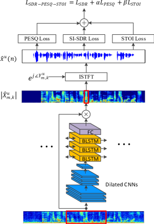
Figure 1: Illustration of End-to-End Multi-Task Denoising based on CNN-BLSTM

Figure 1 describes the proposed end-to-end multi-task denoising framework. The underlying model architecture is composed of convolutional layers and bi-directional LSTM. The spectrogram formed by 11 frames of the noisy amplitude spectrum $|Y^{u}_{m,k}|$ is the input to the convolutional layers. $u$ is an utterance index, $m$ is a frame index and $k$ is a frequency index. The dilated convolution with rate of 2 and 4 is applied to the second and third layers, respectively, in order to increase kernel’s coverage on frequency bins. Dilation is only applied to the frequency dimension because time correlation will be learned by bi-drectional LSTMs. Griffin-Lim ISTFT [7] is applied to the synthesized complex spectrum $\hat{X}^{u}_{m,k}$ to obtain time-domain denoised output $\hat{x}^{u}(n)$. Three proposed loss functions are evaluated based on $\hat{x}^{u}(n)$ and therefore, they are free from the spectrum mismatch.

2.1 SDR Loss Function

Unlike SNR, the definition of SDR is not unique. There are at least two popularly used SDR definitions. The most well known Vincent’s definition [8] is given by

$$\textrm{SDR}^{u}=10\log_{10}\frac{||x^{u}_{target}||^{2}}{||e^{u}_{noise}+e^{u}_{artif}||^{2}}$$ (1)

$x^{u}_{target}$ and $e^{u}_{noise}$ can be found by projecting the denoised signal $\hat{x}^{u}(n)$ into the clean and noise signal domains, respectively. $e^{u}_{artif}$ is a residual term. They can be formulated as follows:

$$x^{u}_{target} = \frac{(x^{u})^{T}\hat{x}^{u}}{||x^{u}||^{2}}x^{u}$$ (2)

$$e^{u}_{noise} = \frac{(n^{u})^{T}\hat{x}^{u}}{||n^{u}||^{2}}n^{u}$$ (3)

$$e^{u}_{artif} = \hat{x}^{u}-\left(\frac{(x^{u})^{T}\hat{x}^{u}}{||x^{u}||^{2}}x^{u}+\frac{(n^{u})^{T}\hat{x}^{u}}{||n^{u}||^{2}}n^{u}\right)$$ (4)

Substituting Eq.(2), (3) and (4) into Eq.(1), the rearranged SDR is given by

$$\textrm{SDR}^{u} = 10\log_{10}\frac{||\alpha^{u}x^{u}||^{2}}{||\alpha^{u}x^{u}-\hat{x}^{u}||^{2}}$$ (5)

where $\alpha^{u}=\operatorname*{arg\,min}_{\alpha}||\alpha x^{u}-\hat{x}^{u}||=\frac{(x^{u})^{T}\hat{x}^{u}}{||x^{u}||^{2}}x^{u}$. Eq. (5) coincides with scale-invariant SDR (SI-SDR), which is another popularly used SDR definition [9]. In the general multiple source denoising problems, SDR and SI-SDR do not match each other. However, for the single source denoising problem, we can use them interchangeably. SDR loss function is defined as mini-batch average of Eq.(5):

$$\textrm{L}_{\textrm{SDR}}=\frac{1}{B}\sum_{u=0}^{B-1}10\log_{10}\frac{||\alpha^{u}x^{u}||^{2}}{||\alpha^{u}x^{u}-\hat{x^{u}}||^{2}}$$ (6)

where $\alpha$ is $\frac{(x^{u})^{T}\hat{x^{u}}}{||x^{u}||^{2}}$. Figure 2 illustrates why training $\alpha$ is important to maximize the SDR metric. For two noisy signals $y_{1}$ and $y_{2}$, they have the same SNR of $\frac{||x||^{2}}{||x-y_{1}||^{2}}=\frac{||x||^{2}}{||x-y_{2}||^{2}}$ because they are positioned at the same circle centered at the clean signal $x$. However, their SDRs are different. For $y_{1}$, SDR is $\frac{||\alpha_{1}x||^{2}}{||\alpha_{1}x-y_{1}||^{2}}$, which is $\frac{||x||^{2}}{||x-\beta_{1}y_{1}||^{2}}$ by geometry. By the same way, SDR for $y_{2}$ is $\frac{||x||^{2}}{||x-\beta_{2}y_{2}||^{2}}$. Clearly, $y_{1}$ is better than $y_{2}$ in terms of SDR metric, but the MSE criterion cannot distinguish between them because they have the same SNR.

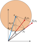
Figure 2: SDR comparison between two noisy signals with the same SNR

2.2 PESQ Loss Function

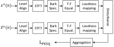
Figure 3: Block Diagram for the PESQ loss function: $x^{u}(n)$ and $\hat{x}^{u}(n)$ are clean and denoised time-domain signals.

PESQ [10] is defined by ITU-T recommendation P.862 for the objective speech quality evaluation. Figure 3 shows the block diagram to find PESQ loss function $\textrm{L}_{\textrm{PESQ}}$. The overall procedure is similar to the PESQ system in  [10]. There are three major modifications. First, the IIR filter in the PESQ calculation is removed. The reason is that time evolution of IIR filter is too deep to apply back-propagation. Second, delay adjustment routine is not necessary because training data pairs were already time-aligned. Third, bad-interval iteration is removed. As long as clean and noisy data pairs are time-aligned, there’s no substantial impact on PESQ from removing it. Each block in Figure 3 is briefly explained below:

Level Alignment: The average power of clean and noisy speech ranging from 300Hz to 3KHz are set to be predefined power value, $10^{7}$.

Bark Spectrum: The Bark spectrum block is to convert linear scale frequency bins into the Bark scale which is roughly equivalent to a logarithmic scale. The mapped bark spectrum power can be formulated as follows:

$$B^{u}_{c,m,i}=\frac{1}{I_{i+1}-I_{i}}\sum_{k=I_{i}}^{I_{i+1}-1}|X^{u}_{m,k}|^{2}$$ (7)

where $I_{i}$ is the start of linear frequency bin number for the $i^{th}$ bark spectrun, $B^{u}_{c,m,i}$ is $i^{th}$ bark spectrum power of clean speech. All the positive linear frequency bins were mapped to 49 Bark spectrum bins. $B^{u}_{n,m,i}$ is a bark spectrum power of noisy speech and can be also found in the similar manner.

Time-Frequency Equalization: Each Bark spectrum bin of clean speech is compensated by the average power ratio between clean and noisy Bark spectrum as follows

$$E^{u}_{c,m,i}=\frac{P^{u}_{n,i}+c_{1}}{P^{u}_{c,i}+c_{1}}B^{u}_{c,m,i}$$ (8)

where $P^{u}_{n,i}=\frac{1}{M_{u}}\sum_{m=0}^{M_{u}-1}B^{u}_{n,m,i}S^{u}_{n,m,i}$ and $P^{u}_{c,i}=\frac{1}{M_{u}}\sum_{m=0}^{M_{u}-1}B^{u}_{c,m,i}S^{u}_{c,m,i}$. $S^{u}_{c,m,i}$ and $S^{u}_{n,m,i}$ are silence masks for clean and noisy speech, respectively. They are fixed arrays of thresholds intended to avoid frequency compensation for the region where clean or noisy speech powers were small. 49 entries of silence masks are defined in PESQ source code [11]. $c_{1}$ is a small constant whose main purpose is to avoid division by zero. It is currently set as 1000. A noise bark spectrum is also similarly compensated for each frame.

Loudness Mapping: The power densities are transformed to a Soner loudness scale using Zwicker’s law [12]:

$$L^{u}_{x,m,i}=S_{i}\left(\frac{P_{0,i}}{0.5}\right)\left[\left(0.5+0.5\frac{E^{u}_{x,m,i}}{P_{0,i}}\right)-1\right]$$ (9)

where $P_{0,i}$ is the absolute hearing threshold, $S_{i}$ is the loudness scaling factor, and r is Zwicker power and x can be c (clean) or n (noisy).

Disturbance Processing: The raw disturbance is difference between clean and noisy loudness densities with following operations:

$$D^{u}_{m,i}=\max\left(L^{u}_{c,m,i}-L^{u}_{n,m,i}-\textrm{DZ}^{u}_{m,i},0\right)$$

$$+\min\left(L^{u}_{c,m,i}-L^{u}_{n,m,i}+\textrm{DZ}^{u}_{m,i},0\right)$$ (10)

where $\textrm{DZ}^{u}_{m,i}=0.25\min(L^{u}_{c,m,i},L^{u}_{n,m,i})$. If absolute difference between clean and noisy loudness densities are less than 0.25 of minimum of two densities, raw disturbance becomes zero. From raw disturbance, symmetric frame disturbance is given by

$$\textrm{FD}^{u}_{m}=\sqrt{\frac{1}{\sum_{i=0}^{I-1}w_{i}}\sum_{i=0}^{I-1}\left(w_{i}D^{u}_{m,i}\right)^{2}}$$ (11)

where $w_{i}$ is predefined weighting for bark spectrum bins. It is also defined in PESQ source code [11]. Asymmetric frame disturbance has additional scaling and thresholding steps as follows:

$$h^{u}_{m,i} = \left(\frac{B^{u}_{n,m,i}+50}{B^{u}_{c,m,i}+50}\right)^{1.2}$$ (12)

$$h^{u}_{m,i} = \bigg{\{}\begin{array}[]{l}12,\textrm{ if }h^{u}_{m,i}>12\\ 0,\textrm{ if }h^{u}_{m,i}<3\end{array}$$ (15)

$$\textrm{AFD}^{u}_{m}=\sqrt{\frac{1}{\sum_{i=0}^{I-1}w_{i}}\sum_{i=0}^{I-1}\left(w_{i}D^{u}_{m,i}h^{u}_{m,i}\right)^{2}}$$ (16)

Aggregation: PESQ loss function $L_{\textrm{PESQ}}$ can be found as follows:

$$L_{\textrm{PESQ}}=4.5-0.1d_{sym}-0.0309d_{asym}$$ (17)

$d_{sym}$ can be found from two stage averaging:

$$\textrm{PSQM}_{s}^{u}=\sqrt[6]{\frac{1}{20}\sum_{i=0}^{19}\left(\textrm{FD}^{u}_{10s+i}\right)^{6}}$$ (18)

$$d_{sym}=\frac{1}{B}\sum_{u=0}^{B-1}\sqrt{\frac{1}{S^{u}}\sum_{s=0}^{S^{u}-1}\left(\textrm{PSQM}_{s}^{u}\right)^{2}}$$ (19)

where $S^{u}$ is $\lfloor\frac{M^{u}}{10}\rfloor$. $d_{asym}$ can also be found with similar averaging using $\textrm{AFD}^{u}_{m}$ instead of $\textrm{FD}^{u}_{m}$.

Table 1: SDR and PESQ results on QUT-NOISE-TIMIT: Test set consists of 6 SNR ranges:-10, -5, 0, 5, 10, 15 dB. The highest SDR or PESQ scores for each SNR test data were highlighted with bold fonts.

	SDR						PESQ
Loss Type	-10dB	-5dB	0dB	5dB	10dB	15dB	-10dB	-5dB	0dB	5dB	10dB	15dB
Noisy Input	-11.82	-7.33	-3.27	0.21	2.55	5.03	1.07	1.08	1.13	1.26	1.44	1.72
IAM	-3.23	0.49	2.79	4.63	5.74	7.52	1.29	1.47	1.66	1.88	2.07	2.30
PSM	-2.95	0.92	3.37	5.40	6.64	8.50	1.30	1.49	1.71	1.94	2.15	2.37
SDR	-2.66	1.55	4.13	6.25	7.53	9.39	1.26	1.42	1.65	1.92	2.16	2.41
SDR-STOI	-2.45	1.67	4.22	6.38	7.62	9.56	1.30	1.49	1.72	1.99	2.21	2.49
SDR-PESQ	-2.31	1.80	4.36	6.51	7.79	9.65	1.43	1.65	1.89	2.16	2.35	2.54
SDR-PESQ-STOI	-2.34	1.78	4.22	6.37	7.54	9.36	1.37	1.59	1.83	2.13	2.37	2.61

Table 2: STOI results on QUT-NOISE-TIMIT

Loss Type	-10dB	-5dB	0dB	5dB	10dB	15dB
Noisy Input	51.9	60.4	68.6	76.9	82.4	86.9
SDR	58.5	70.8	79.0	84.6	87.3	89.6
SDR-PESQ	60.6	72.6	80.4	85.6	88.2	90.3
SDR-STOI	60.6	72.5	80.2	85.5	88.1	90.3
SDR-PESQ-STOI	60.8	73.0	80.6	85.7	88.3	90.3

Table 3: Evaluation on VoiceBank-DEMAND corpus

Models	CSIG	CBAK	COVL	PESQ	SSNR	SDR
Noisy Input	3.37	2.49	2.66	1.99	2.17	8.68
SEGAN	3.48	2.94	2.80	2.16	7.73	-
WAVENET	3.62	3.23	2.98	-	-	-
TF-GAN	3.80	3.12	3.14	2.53	-	-
SDR-PESQ (ours)	4.09	3.54	3.55	3.01	10.44	19.14

2.3 STOI Loss Function

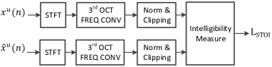
Figure 4: Block Diagram for the STOI loss function

STOI [13, 14] is a segmented correlation-based metric. STOI optimized the segment length that provides the highest correlation with the speech intelligibility. The experiment result of Figure 10 in [13] showed STOI gets the highest correlation for segment lengths around hundreds of milliseconds. The analysis window length of $384$ ms is chosen based on this criterion.

The proposed STOI loss function is depicted in Figure 4. The clean and denoised signal pairs are converted into complex spectra vis STFT. After linear frequency scale is converted into 1/3-octave frequency scale, a noisy spectrum is normalized and clipped by the norm of a clean spectrum. The intelligibility measure is calculated by correlation between normalized clean and noisy spectra. Finally, $\textrm{L}_{\textrm{STOI}}$ is averaged over 1/3 octave bands, frames and mini-batch utterances:

$$\textrm{L}_{\textrm{STOI}}=\frac{1}{BMJ}\sum_{u=0}^{B-1}\sum_{m=0}^{M-1}\sum_{j=0}^{J-1}d_{m,j}^{u}$$ (20)

where B is the number of mini-batch utterances, M is the number of frames, J is the number of 1/3 octave bands and $d_{m,j}^{u}$ is intelligibility measure at utterance $u$, frame $m$ and 1/3-octave band $j$ which is described in detail at Eq. (5) in [13].

2.4 Joint optimization of perceptual speech metrics

In this section, several new loss functions are defined by combining SDR, PESQ and STOI loss functions. The first one is to jointly maximize SDR and PESQ by combining $L_{\textrm{SDR}}$ and $\textrm{L}_{\textrm{PESQ}}$:

$$\textrm{L}_{\textrm{SDR-PESQ}}=\textrm{L}_{\textrm{SDR}}+\alpha\textrm{L}_{\textrm{PESQ}}$$ (21)

where $\alpha$ is a hyper-parameter to adjust relative weighting between SDR and PESQ loss functions.

Similarly, SDR and STOI can be jointly maximized by combining $L_{\textrm{SDR}}$ and $\textrm{L}_{\textrm{STOI}}$ as follows:

$$\textrm{L}_{\textrm{SDR-STOI}}=\textrm{L}_{\textrm{SDR}}+\beta\textrm{L}_{\textrm{STOI}}$$ (22)

where $\beta$ is a hyper-parameter to adjust relative weighting between SDR and STOI loss functions.

Finally, we can combine all three loss functions to jointly optimize SDR, PESQ and STOI metrics as follows:

$$\textrm{L}_{\textrm{SDR-PESQ-STOI}}=\textrm{L}_{\textrm{SDR}}+\alpha\textrm{L}_{\textrm{STOI}}+\beta\textrm{L}_{\textrm{STOI}}$$ (23)

3 Experimental Results

3.1 Experimental Settings

Two datasets were used for the evaluation of the proposed denoising framework. QUT-NOISE-TIMIT [15] is synthesized by mixing 5 different background noise sources with the TIMIT [16]. For the training set, -5 and 5 dB SNR data were used but the evaluation set contains all SNR ranges. The total length of train and test data corresponds to 25 hours and 12 hours, respectively. For VoiceBank-DEMAND [17], 30 speakers selected from Voice Bank corpus [18] were mixed with 10 noise types:8 from Demand dataset [19] and 2 artificially generated one. Test set is generated with 5 noise types from Demand.

3.2 Main Result

Table 1 compared SDR and PESQ performance between different denoising methods on QUT-NOISE-TIMIT corpus. All the schemes were based on the same CNN-BLSTM model trained with -5 and +5 dB SNR data. IAM and PSM are the existing spectral mask estimation schemes. SDR refers to $\textrm{L}_{\textrm{SDR}}$ at Section 2.1 and SDR-PESQ, SDR-STOI and SDR-PESQ-STOI correspond to $\textrm{L}_{\textrm{SDR-PESQ}}$, $\textrm{L}_{\textrm{SDR-STOI}}$ and $\textrm{L}_{\textrm{SDR-PESQ-STOI}}$ at Section 2.4, respectively.

$\textrm{L}_{\textrm{SDR}}$ outperformed IAM and PSM for all SNR ranges in terms of SDR metric. However, for PESQ, it did not show similar improvement due to the metric mismatch. $\textrm{L}_{\textrm{SDR-PESQ}}$ loss function improved both SDR and PESQ metrics. $\textrm{L}_{\textrm{PESQ}}$ loss function acted as a regularization term to improve not only PESQ but also the SDR metric. The STOI loss function was not as effective as PESQ loss function to improve PESQ and SDR metrics. SDR-STOI and SDR-PESQ-STOI showed degradation on the SDR metric compared with SDR-PESQ.

Table 2 compared STOI performance among different loss functions. $\textrm{L}_{\textrm{SDR-STOI}}$ loss function showed $1.52$% relative STOI gain over the SDR loss function. One thing to note is that $\textrm{L}_{\textrm{SDR-PESQ}}$ showed the similar improvement on STOI as $\textrm{L}_{\textrm{SDR-SI}}$, which is a surprising result because the model based on $\textrm{L}_{\textrm{SDR-PESQ}}$ was not directly trained with STOI function but its generalization on the STOI metric is as good as the model based on $\textrm{L}_{\textrm{SDR-STOI}}$. We further evaluated STOI performance by combining all three loss functions. However, $\textrm{L}_{\textrm{SDR-PESQ-STOI}}$ showed only marginal STOI improvements over $\textrm{L}_{\textrm{SDR-PESQ}}$. Considering the result on SDR and PESQ metrics, $\textrm{L}_{\textrm{SDR-PESQ}}$ loss function showed the most consistent performance over all three metrics.

3.3 Comparison with Generative Models

Table 3 showed comparison with other generative models. All the results except our end-to-end model came from the original papers: SEGAN [4], WAVENET [20] and TF-GAN [5]. CSIG, CBAK and COVL are objective measures, where high value means better quality of speech [21]. CSIG is mean opinion score (MOS) of signal distortion, CBAK is MOS of background noise intrusiveness and COVL is MOS of the overall effect. SSNR is Segmental SNR defined in [22].

The proposed SDR and PESQ joint optimization scheme outperformed all the generative models in all the perceptual speech metrics listed above. One thing to note is that any of the metrics at Table 3 was not used as a loss function but the proposed SDR and PESQ combined loss function is highly effective to those metrics, which suggested its good generalization performance.

4 Conclusion

In this paper, a new end-to-end multi-task denoising scheme was proposed. The proposed scheme resolved two issues addressed before: spectrum and metric mismatches. The experimental result presented that the proposed joint optimization scheme significantly improved SDR, PESQ and STOI performances over both spectral mask estimation schemes and generative models. Moreover, the proposed scheme provided good generalization performance by showing substantial improvement on the unseen perceptual speech metrics.

References

- [1] A. Narayanan and D. Wang, “Ideal ratio mask estimation using deep neural networks for robust speech recognition,” in Acoustics, Speech and Signal Processing (ICASSP), 2013 IEEE International Conference on. IEEE, 2013, pp. 7092–7096.
- [2] Y. Wang, A. Narayanan, and D. Wang, “On training targets for supervised speech separation,” IEEE/ACM Transactions on Audio, Speech and Language Processing (TASLP), vol. 22, no. 12, pp. 1849–1858, 2014.
- [3] H. Erdogan, J. R. Hershey, S. Watanabe, and J. Le Roux, “Phase-sensitive and recognition-boosted speech separation using deep recurrent neural networks,” in Acoustics, Speech and Signal Processing (ICASSP), 2015 IEEE International Conference on. IEEE, 2015, pp. 708–712.
- [4] S. Pascual, A. Bonafonte, and J. Serra, “Segan: Speech enhancement generative adversarial network,” arXiv preprint arXiv:1703.09452, 2017.
- [5] M. H. Soni, N. Shah, and H. A. Patil, “Time-frequency masking-based speech enhancement using generative adversarial network,” 2018.
- [6] J. B. Allen and L. R. Rabiner, “A unified approach to short-time fourier analysis and synthesis,” Proceedings of the IEEE, vol. 65, no. 11, pp. 1558–1564, 1977.
- [7] D. Griffin and J. Lim, “Signal estimation from modified short-time fourier transform,” IEEE Transactions on Acoustics, Speech, and Signal Processing, vol. 32, no. 2, pp. 236–243, 1984.
- [8] E. Vincent, R. Gribonval, and C. Févotte, “Performance measurement in blind audio source separation,” IEEE transactions on audio, speech, and language processing, vol. 14, no. 4, pp. 1462–1469, 2006.
- [9] J. L. Roux, S. Wisdom, H. Erdogan, and J. R. Hershey, “Sdr-half-baked or well done?” arXiv preprint arXiv:1811.02508, 2018.
- [10] A. W. Rix, J. G. Beerends, M. P. Hollier, and A. P. Hekstra, “Perceptual evaluation of speech quality (pesq)-a new method for speech quality assessment of telephone networks and codecs,” in Acoustics, Speech, and Signal Processing, 2001. Proceedings.(ICASSP’01). 2001 IEEE International Conference on, vol. 2. IEEE, 2001, pp. 749–752.
- [11] “Perceptual evaluation of speech quality (pesq): An objective method for end-to-end speech quality assessment of narrow-band telephone networks and speech codecs,” ITU-T Recommendation P.862, 2001.
- [12] E. Zwicker and R. Feldtkeller, Das Ohr als Nachrichtenempfänger. Hirzel, 1967.
- [13] C. H. Taal, R. C. Hendriks, R. Heusdens, and J. Jensen, “An algorithm for intelligibility prediction of time–frequency weighted noisy speech,” IEEE Transactions on Audio, Speech, and Language Processing, vol. 19, no. 7, pp. 2125–2136, 2011.
- [14] Y. Zhao, B. Xu, R. Giri, and T. Zhang, “Perceptually guided speech enhancement using deep neural networks,” in 2018 IEEE International Conference on Acoustics, Speech and Signal Processing (ICASSP). IEEE, 2018, pp. 5074–5078.
- [15] D. B. Dean, S. Sridharan, R. J. Vogt, and M. W. Mason, “The qut-noise-timit corpus for the evaluation of voice activity detection algorithms,” Proceedings of Interspeech 2010, 2010.
- [16] J. S. Garofolo, L. F. Lamel, W. M. Fisher, J. G. Fiscus, and D. S. Pallett, “Darpa timit acoustic-phonetic continous speech corpus cd-rom. nist speech disc 1-1.1,” NASA STI/Recon technical report n, vol. 93, 1993.
- [17] C. Valentini, X. Wang, S. Takaki, and J. Yamagishi, “Investigating rnn-based speech enhancement methods for noise-robust text-to-speech,” in 9th ISCA Speech Synthesis Workshop, 2016, pp. 146–152.
- [18] C. Veaux, J. Yamagishi, and S. King, “The voice bank corpus: Design, collection and data analysis of a large regional accent speech database,” in Oriental COCOSDA held jointly with 2013 Conference on Asian Spoken Language Research and Evaluation (O-COCOSDA/CASLRE), 2013 International Conference. IEEE, 2013, pp. 1–4.
- [19] J. Thiemann, N. Ito, and E. Vincent, “The diverse environments multi-channel acoustic noise database: A database of multichannel environmental noise recordings,” The Journal of the Acoustical Society of America, vol. 133, no. 5, pp. 3591–3591, 2013.
- [20] D. Rethage, J. Pons, and X. Serra, “A wavenet for speech denoising,” in 2018 IEEE International Conference on Acoustics, Speech and Signal Processing (ICASSP). IEEE, 2018, pp. 5069–5073.
- [21] Y. Hu and P. C. Loizou, “Evaluation of objective quality measures for speech enhancement,” IEEE Transactions on audio, speech, and language processing, vol. 16, no. 1, pp. 229–238, 2008.
- [22] S. R. Quackenbush, “Objective measures of speech quality (subjective).” 1986.