A Conservative Discontinuous Galerkin Discretization for the Total Energy Formulation of the Reacting Navier Stokes Equations

Abstract

This paper describes the total energy formulation of the compressible reacting Navier-Stokes equations which is solved numerically using a fully conservative discontinuous Galerkin finite element method (DG). Previous applications of DG to the compressible reacting Navier-Stokes equations required nonconservative fluxes or stabilization methods in order to suppress unphysical oscillations in pressure that led to the failure of simple test cases. In this paper, we demonstrate that material interfaces with a temperature discontinuity result in unphysical pressure oscillations if the species internal energy is nonlinear with respect to temperature. We demonstrate that a temperature discontinuity is the only type of material interface that results in unphysical pressure oscillations for a conservative discretization of the total energy formulation. Furthermore, we demonstrate that unphysical pressure oscillations will be generated at any material interface, including material interfaces where the temperature is continuous, if the thermodynamics are frozen during the temporal integration of the conserved state. Additionally, we demonstrate that the oscillations are amplified if the specific heat at constant pressure is incorrectly evaluated directly from the NASA polynomial expressions. Instead, the mean value, which we derive in this manuscript, should be used to compute the specific heat at constant pressure. This can reduce the amplitude of, but not prevent, unphysical oscillations where the species concentrations numerically mix. We then present solutions to several test cases using a fully conservative DG discretization of the total energy formulation. The test cases demonstrate that this formulation does not generate spurious pressure oscillations for material interfaces if the temperature is continuous and that it is better behaved than frozen thermodynamic formulations if the temperature is discontinuous.

1 Background

The discontinuous Galerkin finite element method (DG) [1, 2, 3, 4, 5, 6, 7, 8, 9, 10, 11, 12], has been applied to the field of computational fluid dynamics with great success over the past two decades. The method is fully conservative, able to achieve high-order accuracy on unstructured grids, and has a well-developed theory of adjoint consistency [13, 14, 12, 15], which makes it a powerful tool for adjoint-based optimization. Furthermore, an extension of DG, the Moving Discontinuous Galerkin Method with Interface Condition Enforcement (MDG-ICE) [16, 17], maintains high order accuracy for flows with interfaces and sharp gradients.

Recent work has shown success in modeling combustion systems using DG [18, 19]. In these previous works, nonphysical pressure oscillations were generated for continuous profiles of species and temperature with constant velocity and pressure. These oscillations have been attributed to variations in the thermodynamic properties of multicomponent gases and it was previously concluded that any fully conservative Godunov-type scheme would be unable to maintain a pressure equilibrium across the material fronts [20]. This was shown conclusively for formulations that used variable ratio of specific heats, $\gamma$, where $\gamma$ was a function of species concentrations [21, 22].

A nonconservative flux, referred to as the double flux method, was implemented to avoid these oscillations in multicomponent reacting flows [23, 24, 18, 19]. The method assumes consistent fluid thermal properties through a material interface, and thereby breaks energy conservation to achieve the desired stability. This method has been successfully applied to multidimensional reacting flow problems, including detonations, and has been shown to be stable [25, 19]. Other methods, such as increasing the size of the state and solving for additional transport equations, have also been employed to avoid these unwanted oscillations in multicomponent flows [26, 27, 28, 29, 30].

In this work, we present the total energy formulation of the reacting Navier-Stokes equations to simulate multicomponent flows that is suitable for conservative DG discretizations. The formulation avoids unwanted pressure oscillations without the need for nonconservative fluxes or other stabilization methods by solving for temperature at each degree of freedom such that the internal energy of the conserved fluid is consistent with the mixture-averaged, temperature-based polynomial expression for internal energy. This formulation is used to approximate solutions to various test cases with material interfaces. The results confirm that pressure oscillations are only generated at material interfaces if the temperature is discontinuous. Additionally, we demonstrate that unphysical pressure oscillations will be generated at any material interface, including material interfaces where the temperature is continuous, if the thermodynamics are frozen during the temporal integration of the conserved state. Furthermore, we present verification for a steady flame, demonstrating the ability of the method to model the desired physics in combustion systems with high order accuracy without generating pressure oscillations.

2 Formulations

2.1 The Total Energy Formulation

The nonlinear conservation law, given in strong form, defined for piecewise smooth, $\mathbb{R}^{m}$-valued functions $y$, and gradient $\nabla y$, is

$$\frac{\partial y}{\partial t}+\nabla\cdot\mathcal{F}\left(y,\nabla y\right)-\mathcal{S}\left(y\right)=0 \textup{ in }\Omega,$$ (2.1)

$$y\left(\cdot,t_{0}\right)-y_{0}=0 \textup{ in }\Omega,$$ (2.2)

$$n\cdot\mathcal{F}\left(y,\nabla y\right)-n\cdot\mathcal{F}_{\Gamma}\left(y_{\Gamma},\nabla y\right)=0 \textup{ in }\Gamma,$$ (2.3)

for a given flux function $\mathcal{F}:\mathbb{R}^{m}\rightarrow\mathbb{R}^{m\times n}$ and source term $\mathcal{S}:\mathbb{R}^{m}\rightarrow\mathbb{R}^{m}$, where $\Omega\subset\mathbb{R}^{n}$ is a given spatial domain and $t$ denotes time. The initial conditions are given by $y_{0}$ in Eq. (2.2), while the boundary conditions in Eq. (2.3) are imposed through the boundary flux, $\mathcal{F}_{\Gamma}\left(y_{\Gamma},\nabla y\right)=h_{\Gamma}\left(y\right)-\mathcal{F}_{\Gamma}^{\nu}\left(y_{\Gamma},\nabla y\right)$, where $h_{\Gamma}\left(y\right)$ and $\mathcal{F}_{\Gamma}^{\nu}\left(y_{\Gamma},\nabla y\right)$ are the numerical and viscous fluxes, respectively, at the boundary. The flux function

$$F\left(y,\nabla y\right)=\left(\mathcal{F}^{c}\left(y\right)-\mathcal{F}^{v}\left(y,\nabla y\right)\right)$$ (2.4)

is defined in terms of the convective flux $\mathcal{F}^{c}\left(y\right)$, which is only a function of the state $y$, and viscous flux $\mathcal{F}^{v}\left(y,\nabla y\right)$, which is a function of the state and the gradient, $\nabla y$. The reacting Navier-Stokes flow state variable is given by

$$y=\left(\rho v_{1},\ldots,\rho v_{n},\rho e_{t},C_{i},\ldots,C_{n_{s}}\right)\in\mathbb{R}^{m},$$ (2.5)

where $m=n+n_{s}+1$, $n$ is the number of spatial dimensions, $n_{s}$ is the number of thermally perfect species, $\rho$ is density, $\left(v_{1},\ldots,v_{n}\right)\in\mathbb{R}^{n}$ is velocity, $e_{t}$ is the specific total energy, and $C_{i}$ is the concentration of species $i$. The density is calculated from the concentrations as

$$\rho=\sum_{i=1}^{n_{s}}W_{i}C_{i},$$ (2.6)

where $W_{i}$ is the molecular weight of species $i$.

The $k$-th spatial convective flux component is given by

$$\mathcal{F}_{k}^{c}\left(y\right)=\left(\rho v_{k}v_{1}+p\delta_{k1},\ldots,\rho v_{k}v_{n}+p\delta_{kn},v_{k}\left(\rho e_{t}+p\right),v_{k}C_{1},\ldots,v_{k}C_{n_{s}}\right)\in\mathbb{R}^{m}.$$ (2.7)

The pressure is calculated from the equation of state,

$$p=R^{o}T\sum_{i=1}^{n_{s}}C_{i},$$ (2.8)

where $T$ is the temperature and $R^{o}$ is the universal gas constant, $8314.4621$ J/Kmol/K. The total energy in Eq. (2.5) is related to kinetic and internal energy by

$$\rho e_{t}=\rho u+\frac{1}{2}\sum_{k=1}^{n}\rho v_{k}v_{k},$$ (2.9)

where $\rho u$ is a mass weighted sum of thermally perfect species specific internal energies that are $n_{p}$-order polynomials with respect to temperature,

$$\rho u=\sum_{i=1}^{n_{s}}W_{i}C_{i}\sum_{k=0}^{n_{p}}a_{ik}T^{k}.$$ (2.10)

The $k$-th spatial component of the viscous flux is given by

$$\mathcal{F}_{k}^{v}\left(y,\nabla y\right)=\left(0,\tau_{1k},\ldots,\tau_{nk},\tau_{kj}v_{j}-W_{i}C_{i}h_{i}V_{ik}+\lambda\frac{\partial T}{\partial x_{k}},C_{1}V_{1k},\ldots,C_{n_{s}}V_{n_{s}k}\right)\in\mathbb{R}^{m},$$ (2.11)

where $\lambda$ is the thermal conductivity, $\tau\in\mathbb{R}^{n\times n}$ is the viscous stress tensor, $h_{i}$ is the specific enthalpy of species $i$, and $\left(V_{i1},\dots,V_{in}\right)\in\mathbb{R}^{n}$ is the diffusion velocity of species $i$. The $k$-th spatial component of the viscous stress tensor is given by

$$\tau_{k}=\mu\left(\frac{\partial v_{1}}{\partial x_{k}}+\frac{\partial v_{k}}{\partial x_{1}}-\delta_{k1}\frac{2}{3}\sum_{j=1}^{n}\frac{\partial v_{j}}{\partial x_{j}},\ldots,\frac{\partial v_{n}}{\partial x_{k}}+\frac{\partial v_{k}}{\partial x_{n}}-\delta_{kn}\frac{2}{3}\sum_{j=1}^{n}\frac{\partial v_{j}}{\partial x_{j}}\right),$$ (2.12)

where $\mu$ is the dynamic viscosity coefficient and $\left(x_{1},\ldots,x_{n}\right)\in\mathbb{R}^{n}$ are spatial coordinates. The transport properties are calculated using mixture averaged properties. The species diffusion velocity is calculated using the mixture averaged diffusion,

$$V_{ik}=\frac{D_{i}}{C_{i}}\frac{\partial C_{i}}{\partial x_{k}}-\frac{D_{i}}{\rho}\frac{\partial\rho}{\partial x_{k}},$$ (2.13)

where $D_{i}$ is the mixture averaged diffusion coefficient of species $i$ from [31],

$$D_{i}=\frac{p_{atm}}{p\bar{W}}\frac{\sum_{j=1,j\neq i}^{n_{s}}X_{j}W_{j}}{\sum_{j=1,j\neq i}^{n_{s}}X_{j}/D_{ij}},$$ (2.14)

$p_{atm}=101325$ Pa, $X_{j}$ is the mole fraction of species $j$, $D_{ij}$ is the diffusion coefficient of species $i$ to species $j$, and $\bar{W}$ is the mixture molecular weight, $\bar{W}=\rho/\sum_{i=1}^{n_{s}}C_{i}$. The mole fractions can be calculated directly from concentrations, $X_{i}=C_{i}/\sum_{i=1}^{n_{s}}C_{i}$. The Wilke model [32] is used to calculate viscosity

$$\mu = \sum_{i=1}^{n_{s}}\frac{X_{i}\mu_{i}}{X_{i}+\sum_{i=1,i\neq j}^{n_{s}}\left(X_{j}\phi_{ij}\right)},$$ (2.15)

defined in terms of

$$\phi_{ij} = \frac{\left(1+\left(\frac{W_{j}}{W_{i}}\right)^{1/4}\sqrt{\left(\frac{\mu_{i}}{\mu_{j}}\right)}\right)^{2}}{\sqrt{8\left(1+\frac{W_{i}}{W_{j}}\right)}},$$

where $\mu_{i}$ and $\mu_{j}$ are the species specific viscosities for species $i$ and $j$ respectively. The Mathur model [33] is used to calculate conductivity,

$$\lambda=\frac{1}{2}\left(\sum_{i=1}^{n_{s}}X_{i}\lambda_{i}+\frac{1}{\sum_{i=1}^{n_{s}}\frac{X_{i}}{\lambda_{i}}}\right),$$ (2.16)

where $\lambda_{i}$ is the conductivity of species $i$.

Finally, the source term is given by

$$\mathcal{S}\left(y\right)=\left(0,\ldots,0,0,\omega_{1},\ldots,\omega_{n_{s}}\right)\in\mathbb{R}^{m},$$ (2.17)

where $\omega_{i}$ is the production rate of species $i$. The production rate comes from the sum of the progress reaction rates from any arbitrary number of reactions and reaction types.

2.2 The Ratio of Specific Heats Formulation

Here we present how the ratio of specific heats, $\gamma$, can be used in the total energy formulation, described in Section 2.1, and we present the necessary constraints to keep the two formulations consistent. We seek a formulation analogous to the calorically perfect gas formulation, $\rho u=p/\left(\gamma-1\right)$. To do so we use the definition of internal energy in terms of enthalpy and pressure,

$$\rho u=\rho h-p.$$ (2.18)

Here the enthalpy is

$$\rho h=\rho\sum_{i=1}^{n_{s}}Y_{i}\int_{0}^{T}C_{p,i}dT=\rho\sum_{i=1}^{n_{s}}Y_{i}h_{i},$$ (2.19)

where $Y_{i}$ is the mass fraction of species $i$, $Y_{i}=W_{i}C_{i}/\rho$, $C_{p,i}$ is the specific heat at constant pressure of species $i$, and $h_{i}$ is the species specific enthalpy polynomial of temperature that is degree $n_{p}$, $h_{i}=\sum_{k=0}^{n_{p}}a_{ik}T^{k}+R^{o}T$. We reduce the definition of internal energy to achieve the equivalent formulation that contains a similar expression to $\rho u=\frac{p}{\gamma-1}$ by introducing the mean value from reference temperature, $T_{0}$, to current temperature, $T$, of $\bar{C}_{p,i}$ and $\bar{C}_{p}$ ,

$$\bar{C}_{p,i}=\frac{1}{T-T_{0}}\int_{T_{0}}^{T}C_{p,i}dT=\frac{h_{i}-h_{i}^{0}}{T-T_{0}}$$ (2.20)

and

$$\bar{C}_{p}=\sum_{i=1}^{n_{s}}\frac{Y_{i}}{T-T_{0}}\int_{T_{0}}^{T}C_{p,i}dT=\frac{\sum_{i=1}^{n_{s}}Y_{i}\left(h_{i}-h_{i}^{0}\right)}{T-T_{0}}$$ (2.21)

where $h_{i}^{0}$ is the species specific enthalpy at $T_{0}$. Using the following definitions

$$\bar{\gamma} = \frac{\bar{C}_{p}}{\bar{C}_{p}-R}=\frac{\sum_{i=1}^{n_{s}}\frac{Y_{i}\left(h_{i}-h_{i}^{0}\right)}{T-T_{0}}}{\sum_{i=1}^{n_{s}}\frac{Y_{i}\left(h_{i}-h_{i}^{0}\right)}{T-T_{0}}-R},$$ (2.22)

$$R = \frac{R^{o}\sum_{i=1}^{n_{s}}C_{i}}{\rho},$$ (2.23)

$$\rho u = \frac{p}{\bar{\gamma}-1}+\rho\sum_{i=1}^{n_{s}}Y_{i}\left(h_{i}^{0}-\bar{C}_{p,i}T_{0}\right),$$ (2.24)

the inviscid total energy conservation without reactions becomes

$$\frac{\partial\left(\frac{p}{\bar{\gamma}-1}+\frac{1}{2}\sum_{k=1}^{n}\rho v_{k}v_{k}\right)}{\partial t}+\nabla\cdot\left(\left(\frac{p}{\bar{\gamma}-1}+\frac{1}{2}\sum_{k=1}^{n}\rho v_{k}v_{k}+p\right)\left(v_{1},\dots,v_{n}\right)\right) = 0,$$ (2.25)

where the term $\rho\sum_{i=1}^{n_{s}}Y_{i}\left(h_{i}^{0}-\bar{C}_{p,i}T_{0}\right)$ in Eq. (2.24) is eliminated from Eq. (2.25) by fixing $T_{0}$ to 0 K and multiplying the non-reacting inviscid form of the species conservation equations from Eq. (2.1) by $W_{i}h_{i}^{0}$ and summing over all species conservation equations. Eq. (2.25) is equivalent to the non-reacting inviscid form of the conservation of energy from Eq. (2.1). Eq. (2.25) has the same form of the compressible Euler equations, and therefore is convenient for routines that require the ratio of specific heats, e.g., characteristic boundary conditions [34]. However, those routines require the flow to be non-reacting with constant thermodynamic properties as $\bar{\gamma}$ is assumed to be constant.

3 Material Discontinuities in Multicomponent Flows

A material discontinuity is defined as a discontinuity across which there is no mass flow. The velocity and pressure are constant across the discontinuity but other material quantities are not. In this section we exact solutions for problems involving material interfaces by considering the non-reacting inviscid formulation of Eqs. (2.1)-(2.3) where $\mathcal{F}^{v}\left(y,\nabla y\right)=\left(0,\dots,0\right)$ in Eq. (2.4) and $\mathcal{S}\left(y\right)=\left(0,\ldots,0\right)$ in Eq. (2.1). A discontinuous solution, in one dimension satisfies, the inviscid form of Eqs. (2.1)-(2.3) if the jump in the flux is equal to the product of the jump in the state and the material interface velocity [35],

$$\mathcal{F}\left(y_{r}\right)-\mathcal{F}\left(y_{l}\right)=v_{s}\left(y_{r}-y_{l}\right),$$ (3.1)

where $y_{r}$ is the state on the right of the discontinuity, $y_{l}$ is the state on the left of the discontinuity, and $v_{s}$ is the material velocity normal to the interface.

Below we introduce a material discontinuity by considering a one-dimensional two species discontinuity at $x_{j}$ where the velocity and pressure are constant and the temperature is discontinuous,

$$v = \bar{v},$$

$$C_{1} = \begin{cases}C_{1}^{0}&\text{if }x>x_{j}\\ 0&\text{otherwise}\end{cases},$$

$$C_{2} = \begin{cases}0&\text{if }x<x_{j}\\ C_{2}^{0}&\text{otherwise}\end{cases},$$

$$T = \begin{cases}\eta\bar{T}&\text{if }x<x_{j}\\ \bar{T}&\text{otherwise}\end{cases},$$

$$p = \bar{p.}$$

The species with index $i=1$, species 1, has molecular weight $W_{1}$ and the species with index $i=2$, species 2, has molecular weight $W_{2}$. The initial fluid state from Eq. (2.5) is therefore

$$y\left(x,t=0\right)=\begin{cases}\left(W_{1}C_{1}^{0}\bar{v},\frac{1}{2}W_{1}C_{1}^{0}\bar{v}^{2}+W_{1}C_{1}^{0}\sum_{k=0}^{n_{p}}a_{1k}\bar{T}^{k},C_{1}^{0},0\right)&x>x_{j}\\ \left(W_{2}C_{2}^{0}\bar{v},\frac{1}{2}W_{2}C_{2}^{0}\bar{v}^{2}+W_{2}C_{2}^{0}\sum_{k=0}^{n_{p}}a_{2k}\left(\eta\bar{T}\right)^{k},0,C_{2}^{0}\right)&\text{otherwise}\end{cases}.$$ (3.2)

Substituting the fluid state from Eq. (3.2) in Eq. (3.1) we arrive at the following condition

$$W_{1}C_{1}^{0}\bar{v}^{2}-W_{2}C_{2}^{0}\bar{v}^{2} = v_{s}\left(W_{1}C_{1}^{0}v-W_{2}C_{2}^{0}v\right),$$ (3.3)

$$\left(\frac{1}{2}W_{1}C_{1}^{0}v^{2}+C_{1}^{0}W_{1}\sum_{k=0}^{n_{p}}a_{1k}T^{k}+\bar{p}\right)\bar{v}$$

$$-\left(\frac{1}{2}W_{2}C_{2}^{0}v^{2}+C_{2}^{0}W_{2}\sum_{k=0}^{n_{p}}a_{2k}\left(\eta T\right)^{k}+\bar{p}\right)\bar{v} = v_{s}\left(\frac{1}{2}W_{1}C_{1}^{0}v^{2}+W_{1}C_{1}^{0}\sum_{k=0}^{n_{p}}a_{1k}T^{k}\right.$$ (3.4)

$$\left.-\frac{1}{2}W_{2}C_{2}^{0}v^{2}-W_{2}C_{2}^{0}\sum_{k=0}^{n_{p}}a_{2k}\left(\eta T\right)^{k}\right),$$

$$C_{1}^{0}\bar{v} = v_{s}\left(C_{1}^{0}\right),$$ (3.5)

$$-C_{2}^{0}\bar{v} = v_{s}\left(-C_{2}^{0}\right).$$ (3.6)

Therefore a material discontinuity where velocity and pressure are constant and the temperature is discontinuous satisfies Eqs. (2.1)-(2.3) with $v_{s}=\bar{v}$. A diagram of the space-time solution is shown in Fig. 3.1a.

We now present the effect of a linear discretization on the same two species discontinuity. Using the notation from Abgrall and Karni [23], the inviscid non-reacting conservation equations can be written as

$$\delta\left(\rho v\right)+\nu\Delta\left(\rho v^{2}+p\right)= 0,$$ (3.7)

$$\delta\left(\rho e_{t}\right)+\nu\Delta\left(\left(\rho e_{t}+p\right)v\right)= 0,$$ (3.8)

$$\delta\left(C_{i}\right)+\nu\Delta\left(C_{i}v\right)= 0\text{ for }i=1\dots n_{s},$$ (3.9)

where the inviscid forms of Eqs. (2.1)-(2.3) have been linearized with respect to space and time. Here, $\delta\left(\right)=\left(\right)_{j}^{n+1}-\left(\right)_{j}^{n}$ denotes the temporal change of the state, $\Delta\left(\right)$ denotes spatial variation across the interface $\Delta\left(\right)=\left(\right)_{j}^{n}-\left(\right)_{j-1}^{n}$, and $\nu=\frac{\Delta t}{\Delta x}$ where $\Delta t$ is the chosen time step and $\Delta x$ is the spatial distance across the interface. The material interface is initially between two nodes, $j$ and $j-1$, as depicted at time $t^{n}$ in Fig. 3.1b. Specifically, the initial flow state at $t^{n}$ is

$$y_{j}^{n} = \left(W_{1}C_{1}^{0}\bar{v},\frac{1}{2}W_{1}C_{1}^{0}\bar{v}^{2}+W_{1}C_{1}^{0}\sum_{k=0}^{n_{p}}a_{1k}\bar{T}^{k},C_{1}^{0},0\right),$$ (3.10)

$$y_{j-1}^{n} = \left(W_{2}C_{2}^{0}\bar{v},\frac{1}{2}W_{2}C_{2}^{0}\bar{v}^{2}+W_{2}C_{2}^{0}\sum_{k=0}^{n_{p}}a_{2k}\left(\eta\bar{T}\right)^{k},0,C_{2}^{0}\right).$$ (3.11)

For simplification purposes, we define the initial concentration of species 2 in terms of the initial concentration of species 1 through the constant initial pressure conditions, $p_{j}^{n}=p_{j-1}^{n}=\bar{p}$, and the equation of state, Eq. (2.8),

$$R^{o}\bar{T}C_{1}^{0}=R^{o}\eta\bar{T}C_{2}^{0}\rightarrow C_{2}^{0}=\frac{C_{1}^{0}}{\eta}.$$ (3.12)

The species conservation, Eq. (3.9), gives the concentrations at $t^{n+1}$ in terms of the initial species 1 concentration,

$$C_{1,j}^{n+1} = C_{1}^{0}-\nu\bar{v}C_{1}^{0},$$ (3.13)

$$C_{2,j}^{n+1} = \nu\bar{v}C_{2}^{0}=\nu\bar{v}\frac{C_{1}^{0}}{\eta}.$$ (3.14)

Eqs. (3.13) and (3.14) show that there is numerical mixing of the species at time $t^{n+1}$ and node $j$, as depicted in Fig. 3.1b. This is a departure from the exact solution that satisfies the interface condition, depicted in Fig. 3.1a, and we continue in this section by examining the effect that the numerical mixing of the species concentrations has on the stability of the material interface.

(a) The speed of the material interface is the slope of the trajectory $v_{s}=\bar{v}=\angle$.

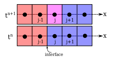
(b) Numerical diffusion of material interface at discrete times.

Figure 3.1: Diagrams of moving material interfaces.

Substituting the concentrations from Eqs. (3.13) and (3.14) into Eq. (2.6) gives the density at $t^{n+1}$,

$$\rho_{j}^{n+1}=\left(W_{1}+\nu\bar{v}\left(\frac{W_{2}}{\eta}-W_{1}\right)\right)C_{1}^{0}.$$ (3.15)

Using Eqs. (3.13)-(3.15) and Eq. (2.6) for the initial density and substituting into Eq. (3.7) reveals that the velocity remains constant,

$$\left(W_{1}+\nu\bar{v}\left(\frac{W_{2}}{\eta}-W_{1}\right)\right)C_{1}^{0}v^{n+1}-W_{1}C_{1}^{0}\bar{v}+\nu\bar{v}^{2}\left(W_{1}C_{1}^{0}-W_{2}\frac{C_{1}^{0}}{\eta}\right) = 0\rightarrow v_{j}^{n+1}=\bar{v}.$$ (3.16)

Using Eqs. (3.13)-(3.16) we consider the change in total energy to analyze the stability of the material interface. We derive a relationship for kinetic energy by multiplying Eq. (3.7) by $\frac{1}{2}\bar{v}$,

$$\left(\frac{1}{2}\rho_{j}^{n+1}\bar{v}^{2}-\frac{1}{2}\rho_{j}^{n}\bar{v}^{2}+\nu\bar{v}\left(\frac{1}{2}\rho_{j}^{n}\bar{v}^{2}-\frac{1}{2}\rho_{j-1}^{n}\bar{v}^{2}\right)\right) = 0,$$ (3.17)

and we derive a relationship for pressure by noting $pv$ is constant across the interface at $t^{n}$,

$$\Delta\left(pv\right) = 0.$$ (3.18)

Combining Eq. (3.17) and Eq. (3.18) with Eq. (3.8) we remove the kinetic energy, contained in $\rho e_{t}=\rho v^{2}/2+\rho u$, and the pressure term to yield a linear relationship for the internal energy across the interface,

$$\delta\rho u+\nu v\Delta\left(\rho u\right) = 0.$$ (3.19)

We substitute Eq. (2.10), Eq. (3.12), and Eqs. (3.13)-(3.15) in Eq. (3.19) and arrive at $n_{p}$ expressions for the temperature at time $t^{n+1}$ by collecting like terms,

$$T_{j}^{n+1} = \bar{T}\frac{\left(W_{1}a_{11}-\nu\bar{v}\left(W_{1}a_{11}-W_{2}a_{21}\right)\right)}{W_{1}\left(1-\nu\bar{v}\right)a_{11}+\frac{W_{2}}{\eta}\left(\nu\bar{v}\right)a_{21}}$$

$$\vdots \vdots \vdots$$

$$\left(T_{j}^{n+1}\right)^{n_{p}} = \left(\bar{T}\right)^{n_{p}}\frac{\left(W_{1}a_{1n_{p}}-\nu\bar{v}\left(W_{1}a_{1N_{p}}-W_{2}a_{2N_{p}}\eta^{n_{p}-1}\right)\right)}{W_{1}\left(1-\nu\bar{v}\right)a_{1n_{p}}+\frac{W_{2}}{\eta}\left(\nu\bar{v}\right)a_{2n_{p}}}.$$ (3.20)

Finally, the change in pressure is given as

$$p_{j}^{n+1}-p_{j}^{n} = R^{o}T_{j}^{n+1}\left(C_{1}^{0}-\nu\bar{v}C_{1}^{0}+\nu\bar{v}\frac{C_{1}^{0}}{\eta}\right)-R^{o}\bar{T}C_{1}^{0}.$$ (3.21)

From analyzing Eqs. (3.20) and (3.21) we come to similar conclusions to those of Jenny et al [36], that pressure oscillations, $p_{j}^{n+1}-p_{j}^{n}\neq 0$, do not exist if one of the following conditions is true

1. The temperature is continuous, $\eta=1$.

2. The contact discontinuity remains grid aligned, $\nu\bar{v}=1$.

3. The contact discontinuity is stationary, $\bar{v}=0$.

4. The internal energies are linear, $n_{p}=1$, with respect to temperature and the species are the same across the interface, i.e., molecular weights are constant across the interface, $W_{1}=W_{2}$, and the internal energies are the same across the interface, $a_{1k}=a_{2k}$.

For condition (1), the numerical mixing of species concentrations, Eqs. (3.13) and (3.14), inside the cell does not cause a pressure oscillation as both species are at the same temperature despite having different internal energies.

When $\eta\neq 1$ the temperature is discontinuous and stabilization, e.g., artificial viscosity, would be required if (2)-(4) were not satisfied. Satisfaction of condition (2) would requires an interface fitting method [16, 17, 37, 38] that dynamically fits a priori unknown discontinuities and is therefore beyond the scope of this manuscript. Condition (3) is a trivial case. Condition (4) applies to ideal gases that have a linear relationship between temperature and internal energy and are assumed to be the same species in all regions of the flow.

Applying the same linearization to Eq. (2.25) we can arrive at a similar relationship for the internal energy based on $\bar{\gamma}$ and $p$,

$$\frac{p_{j}^{n+1}}{\bar{\gamma}_{j}^{n+1}-1} = \frac{\bar{p}}{\bar{\gamma_{1}}-1}-\nu v\left(\frac{\bar{p}}{\bar{\gamma_{1}}-1}-\frac{\bar{p}}{\bar{\gamma}_{2}-1}\right),$$ (3.22)

where $\bar{\gamma}_{1}$ and $\bar{\gamma}_{2}$ are the known specific heat ratios of the right and left hand side based on $C_{1}^{0}$ at temperature $\bar{T}$ and $C_{2}^{0}$ at temperature $\eta\bar{T}$, respectively. The equivalent process for the ratio of specific heats formulation would be to use the definition of pressure and $\bar{\gamma}$ in terms of known concentrations, $C_{1}^{n+1}$, $C_{2}^{n+1}$, $C_{i}^{0}$, and $C_{2}^{0}$, and temperatures, $\eta\bar{T}$ and $\bar{T}$, to solve for $T^{n+1}$. This results in similar nonlinear relationships for temperature but instead from the $h_{i}$ polynomials. It follows that the same stability properties found for the total energy formulation apply to the ratio of specific heats formulation.

4 Numerical Methods

In order to discretize the Eqs. (2.1)-(2.3), the DG method assumes that $\Omega$ can be subdivided into a mesh $\mathcal{T}_{h}=\left\{\kappa\right\}$, consisting of disjoint cells $\kappa$ such that $\bar{\Omega}=\cup_{\kappa\in\mathcal{T}_{h}}\bar{\kappa}$. We also consider $\mathcal{I}_{h}$, consisting of interior interfaces defined between pairs of cells, so that for each $\epsilon\in\mathcal{I}_{h}$, there exists a pair of $\kappa^{+},\kappa^{-}\in\mathcal{T}_{h}$ such that $\epsilon=\kappa^{+}\cap\kappa^{-}$. A discrete subspace, consisting of piecewise polynomials of degree $p$, is defined over $\mathcal{T}_{h}$,

$$V_{h}=\left\{v\mid v\in P^{p}\left(\kappa\right)\text{ for }\kappa\in\mathcal{T}_{h}\left(\Omega\right)\right\}.$$ (4.1)

From this, a DG (semi-)discretization is obtained, find $\frac{\partial y}{\partial t}\in V_{h}$ such that

$$\sum_{\kappa\in\mathcal{T}_{h}}\int_{\kappa}\frac{\partial y}{\partial t}v+\int_{\partial\kappa}\left(h\left(y^{+},y^{-},n\right)\right)v^{+}-\int_{\partial\kappa}\left\{\!\!\left\{\mathcal{F}^{\nu}\left(y,\nabla y\right)\right\}\!\!\right\}\cdot nv^{+}\qquad\qquad\qquad\qquad$$

$$\qquad\qquad\qquad-\int_{\partial\kappa}\delta\left(y^{+},y^{-},n\right)v^{+}-\int_{\kappa}\mathcal{F}\left(y,\nabla y\right)\cdot\nabla v-\int_{\kappa}\mathcal{S}\left(y\right)\cdot v=0\qquad\forall v\in V_{h},$$ (4.2)

where $h\left(y^{+},y^{-},n\right)$ is the numerical flux, choose to be the HLLC approximate Riemann [39], see also Appendix B of  [19],

$$\left\{\!\!\left\{\mathcal{F}^{\nu}\left(y,\nabla y\right)\right\}\!\!\right\}=\frac{1}{2}\left(\mathcal{F}^{\nu}\left(y^{+},\nabla y^{+}\right)+\mathcal{F}^{\nu}\left(y^{-},\nabla y^{-}\right)\right),$$

is the average viscous flux, and $\delta\left(y^{+},y^{-},n\right)$ is a penalty term that is required for stability and is implemented via the BR2 formulation [40, 41, 42]. On the exterior interfaces, $\partial\kappa\notin\mathcal{I}_{h}$, the numerical flux is defined consistently with the imposed boundary condition Eq. (2.3) and

$$\left\{\!\!\left\{\mathcal{F}^{\nu}\left(y,\nabla y\right)\right\}\!\!\right\}=\left(\mathcal{F}^{\nu}\left(y_{\Gamma},\nabla y^{+}\right)\right).$$

The DG space semi-discretization is integrated temporally with a strong-stability-preserving Runge-Kutta method (SSP-RK2) [43]. This discretization of convection and diffusion is combined with a stiff ODE solver for the reaction term via Strang splitting [44].

4.1 Implementation of Thermodynamics

It is important to note that $\bar{C}_{p,i}$, Eq. (2.20), and $\bar{C_{p}}$, Eq. (2.21), from Section 2.2 are not equivalent to the evaluations of $C_{p,i}$ and $C_{p}$ from polynomial expressions, e.g., the analytic form of NASA’s polynomial representations [45]. Rather, $\bar{C}_{p,i}$ and $\bar{C}_{p}$ can be viewed as the mean value of $C_{p,i}$ and $C_{p}$, where $\bar{C_{p}}$ approaches $C_{p}$ as $T-T_{o}\rightarrow 0$. This difference can be shown mathematically by using the following polynomial definitions of specific heat at constant pressure,

$$C_{pi} = \sum_{k=0}^{n_{p}}b_{ik}T^{k}$$ (4.3)

and mixture averaged $C_{p}$,

$$C_{p} = \sum_{i=1}^{n_{s}}Y_{i}\sum_{k=0}^{n_{p}}b_{ik}T^{k}.$$ (4.4)

We arrive at the total enthalpy in polynomial form by integrating of Eqs. (4.3) and (4.4) from $0$ to $T$ and substituting the result into Eq. (2.19),

$$\rho h =\rho\sum_{i=1}^{n_{s}}Y_{i}\left(\int_{0}^{T}C_{p,i}dT\right)= \rho\sum_{i=1}^{n_{s}}Y_{i}\left(\sum_{k=0}^{n_{p}}b_{ik}\frac{T^{k+1}}{k+1}\right).$$ (4.5)

By substituting Eq. (4.5) in Eq. (2.21), we arrive at $\bar{C_{p}}$ in terms of the $C_{pi}$ polynomial coefficients and temperature,

$$\bar{C_{p}}=\frac{\sum_{i=1}^{n_{s}}Y_{i}\left(\sum_{k=0}^{n_{p}}b_{ik}\frac{T^{k+1}}{k+1}-\sum_{k=0}^{n_{p}}b_{ik}\frac{T_{0}^{k+1}}{k+1}\right)}{T-T_{0}}.$$ (4.6)

Therefore, $\bar{C_{p}}$ and $C_{p}$ are only equivalent if $C_{p}$ is constant with respect to temperature, i.e., $n_{p}=0$. Fig. 4.1 shows the difference between $C_{p}$ evaluated from NASA polynomials and $\bar{C_{p}}$ evaluated from Eq. (2.21) using a reference temperature, $T_{o}$, of 200 K and mixture of methane, $CH_{4}$, and oxygen, $O_{2}$. Both $\bar{C_{p}}$ and $C_{P}$ were evaluated at a temperature, $T$, of 300 K and 1000 K with the mixture varying from pure methane to pure oxygen, $X_{CH4}=1-X_{O2}$. The values for $C_{p}$ and $\bar{C_{p}}$ are significantly different at higher temperatures due to the large difference between the actual temperature and the reference temperature, $T-T_{0}$.

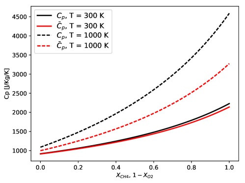
Figure 4.1: The difference between $\bar{C_{p}}$ and $C_{p}$ with reference temperature $T_{0}=200$ K, for a varying mixture of CH4 and O2 at two different temperatures, $T=300$ K and $T=1000$K.

In Section 5 three different methods are used to evaluate the thermodynamics in the convective flux, $\mathcal{F}_{k}^{c}\left(y\right)$, for various test cases. Table 1 shows the steps required to calculate the convective fluxes. The first column corresponds to the total energy formulation that requires the solution of a nonlinear equation for the temperature. The solution ensures equivalency between the computed internal energy and the internal energy given by the evaluation of the corresponding polynomial expression, i.e., find $T$ such that

$$0=\rho u-\sum_{i=1}^{n_{s}}W_{i}C_{i}\sum_{k=1}^{K}a_{ik}T^{k},$$ (4.7)

where the internal energy, $\rho u=\rho e_{t}-\frac{1}{2}\sum_{k=1}^{n}\rho v_{k}v_{k}$, and concentrations, $C_{i}$, are computed from the known state, $y$. In this work the temperature is computed such that the following is satisfied to machine precision for a given an initial temperature:

$$\delta T=\frac{\rho u-\sum_{i=1}^{n_{s}}W_{i}C_{i}\sum_{k=1}^{K}a_{ik}T^{k}}{\frac{\partial\rho u}{\partial T}},$$ (4.8)

where $\delta T$ is the temperature decrement corresponding to Newton’s method and

$$\frac{\partial\rho u}{\partial T}=\sum_{i=1}^{n_{s}}W_{i}C_{i}\sum_{k=1}^{K}ka_{ik}T^{k-1}$$ (4.9)

is the partial derivative of internal energy with respect to temperature. In practice, we observe that the temperature converges within five nonlinear iterations. Once the temperature and state are known, pressure is computed by evaluating Eq. (2.8). The second column of Table 1 corresponds to a frozen thermodynamics evaluation of convective flux where the ratio of specific heats formulation is used and $\bar{\gamma}$ and $\bar{C_{p}}$ are held constant throughout each time step. The third row for the frozen thermodynamics is split into two options. The left corresponds to using $\bar{C_{p}}$ in the evaluation of the flux and the right corresponds to using $C_{p}$, which is evaluated from NASA polynomials expressions.

Table 1: Procedures used to evaluate the convective flux.

Step	Total Energy Formulation	Ratio of Specific Heats Formulation with Frozen Thermodynamics
1	Calculate temperature by solving the nonlinear Eq. (2.9).	Use frozen $\bar{\gamma}$ and $\bar{C_{p}}$ to calculate pressure
2	Calculate pressure from temperature via Eq. (2.8)	Calculate $h_{HLLC}\left(y^{+},y^{-},n\right)$ and $\mathcal{F}_{k}^{c}\left(y\right)$
3	Calculate $h_{HLLC}\left(y^{+},y^{-},n\right)$ and $\mathcal{F}_{k}^{c}\left(y\right)$	Calculate and freeze new $\bar{C_{p}}$ from Eq.  (2.21) and freeze	Calculate and freeze new $\bar{C_{p}}$ as equivalent to $C_{p}$ from Eq.  (4.4) and freeze
4		Calculate and freeze new $\bar{\gamma}$ from $\bar{C_{p}}$ and $R$

If $\bar{\gamma}$ is frozen as presented in the second column in Table 1 then $\gamma_{j}^{n+1}$ in Eq. (3.22) is $\bar{\gamma}_{1}$. A pressure oscillation is now generated regardless of the type of material interface,

$$p_{j}^{n+1}=\bar{p}\left(1-\nu v\left(1-\frac{\bar{\gamma_{1}}-1}{\bar{\gamma}_{2}-1}\right)\right).$$ (4.10)

The freezing of thermodynamics would therefore require other methods to identify and stabilize the nonphysical pressure oscillations even in smooth regions of the flow where $\eta=1$. Previous work showed that pressure oscillations develop even in the presence of continuous temperature profiles which was due to the freezing of thermodynamics [24, 18, 25, 19, 30]. In the following section we explore the magnitude of these pressure oscillations due to frozen thermodynamics and compare to the behavior of the total energy formulation.

5 Test Cases and Verification

In this section we solve several test cases with the total energy formulation and verify the analysis from Section 3. Furthermore, we compare the stability of the total energy formulation to the ratio of specific heats formulation using both frozen $C_{p}$ and frozen $\bar{C_{p}}$. We then verify the total energy formulation by comparing to a one-dimensional premixed hydrogen flame simulation generated by Cantera’s free-flame solver [46]. In the test cases below, the time step is restricted by the Courant-Friedrichs-Lewy number, CFL, defined as

$$\mathrm{CFL}=\frac{\Delta t}{\left(2p+1\right)\min\left(\Delta x\right)}\left(||v||+c\right),$$ (5.1)

where $p$ is the polynomial degree and $c$ is the speed of sound, defined as $c=\sqrt{\gamma RT}$. Here $\gamma$ is the ratio of specific heats which is defined as $\gamma=\frac{C_{p}}{C_{p}-R}$ for both the total energy formulation and the ratio of specific heats formulation with frozen $C_{p}$ and $\gamma=\bar{\gamma}$ for the ratio of specific heats formulation with frozen $\bar{C_{p}}$.

5.1 Discontinuities

We approximate exact solutions corresponding to the discontinuities described in Section 3 by solving the non-reacting, inviscid formulation of the Navier-Stokes Eqs. (2.1)-(2.3) using $\mathrm{DG}(p=1)$, $\mathrm{DG}(p=2)$, and $\mathrm{DG}(p=3)$, without artificial viscosity or limiting. The test problems are run on a periodic domain for one full cycle with $\mathrm{CFL}=0.1$. For each test case we constructed two fictitious species, $n_{s}=2$, with different molecular weights, $W_{1}=20$ and $W_{2}=70$. Here we used a nonlinear function for internal energy, with $n_{p}=3$, $a_{1k}=\{0,2.08e\times 10^{4},83.1,-2.77\times 10^{-2}\}$ and $a_{2k}=\{0,3.33e\times 10^{4},83.1,-2.22\times 10^{-2}\}$, of the form $u_{i}=\sum_{k=0}^{n_{p}}a_{ik}T^{k}$ where $u_{i}$ is the units J/kg with temperature, $T$, in K. The enthalpy of each species is therefore $h_{i}=\sum_{k=0}^{n_{p}}a_{ik}T^{k}+R^{o}T$ and the specific heat at constant pressure of each species is $C_{p,i}=\sum_{k=0}^{n_{p}}ka_{ik}T^{k-1}+R^{o}$. For each test case the domain is $0.1$ m, $\left\{x:x\in\left(0,0.1\right)\right\}$, with grid spacing of $h=0.002$ m. The test cases are solved using both the total energy formulation and the ratio of specific heats formulation with frozen thermodynamics as outlined in Table 1.

5.1.1 Species Discontinuities at Constant Temperature

A species discontinuity at constant temperature, pressure, and velocity, is imposed with the following initial conditions

$$v = 10\textrm{ m/s},$$

$$Y_{1} = \begin{cases}0&\text{if }0.025<x<0.075\\ 1&\text{otherwise}\end{cases},$$

$$Y_{2} = 1-Y_{1},$$

$$T = 300\textrm{ K},$$

$$p = 1\textrm{ atm}.$$

Figs. (5.1a), (5.1b), and (5.1c) show the species mass fractions for the $\mathrm{DG}(p=1)$, $\mathrm{DG}(p=2)$, and $\mathrm{DG}(p=3)$ solutions using the total energy formulation after one cycle. All three solutions present numerical overshoots and mixing of the species mass fractions across the discontinuities. Some of these numerical instabilities cause the mass fractions to be greater than one or negative. As expected, the higher order solutions are more oscillatory for the species mass fractions. Furthermore, larger overshoots are present for the right hand side discontinuity as compared to the left hand side discontinuity.

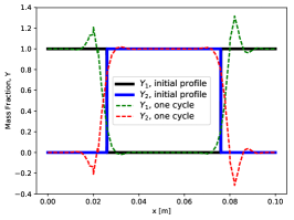
(a) $\mathrm{DG}\left(p=1\right)$ solution

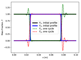
(b) $\mathrm{DG}\left(p=2\right)$ solution

(c) $\mathrm{DG}\left(p=3\right)$ solution

Figure 5.1: Mass fractions for species 1 and 2 for one cycle through domain using the total energy formulation.

Fig. (5.2) shows the pressure after one cycle for the total energy formulation and ratio of specific heats formulations using frozen $\bar{C_{P}}$ and frozen $C_{p}$. The frozen $C_{p}$ solution has pressure oscillations that are on the order of three percent error. Small perturbations of pressure caused by freezing $\bar{C_{p}}$ are shown in Fig. (5.2b). The error caused by the frozen $\bar{C_{p}}$ formulation is reduced as the approximation order is increased from $\mathrm{DG}(p=1)$ to $\mathrm{DG}(p=3)$. In contrast, the pressure for each solution using the total energy formulation maintains a flat profile, which is the expected result from Section 3. The pressure in the total energy solutions never exceed an error of ${1}\mathrm{e}{-7}$ atm.

The corresponding temperature solutions are shown in Figs. (5.3a) and (5.3b). The frozen $C_{p}$ solution gives temperature fluctuations on the order of $1$ K whereas the frozen $\bar{C_{p}}$ solution fluctuates less than $0.025$ K. The total energy solution remains flat and does not exceed ${1}\mathrm{e}{-4}$ K from the expected $300$ K.

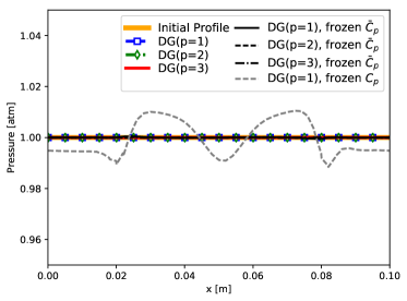
(a) Pressure

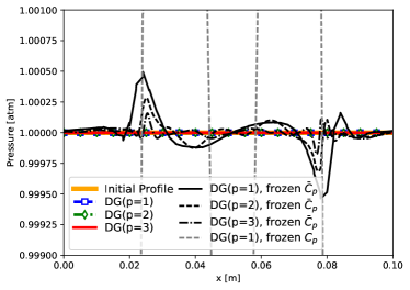
(b) Pressure zoomed view

Figure 5.2: Pressure for $\mathrm{DG}(p=1)$, $\mathrm{DG}(p=2)$, and $\mathrm{DG}(p=3)$ solutions after one cycle.

(a) Temperature

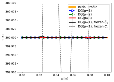
(b) Temperature zoomed view

Figure 5.3: Temperature solutions after one cycle

Figure (5.4a) shows the solutions for $\mathrm{DG}(p=1)$, $\mathrm{DG}(p=2)$, and $\mathrm{DG}(p=3)$ for frozen $\bar{C_{p}}$ at $\mathrm{CFL}$ of $0.1$ and $0.3$. The larger time steps exacerbate the instability introduced by freezing $\bar{C_{p}}$ to exceed 0.001 atm which is still an order of magnitude less than the error of the frozen $C_{p}$ solutions. The solutions for the total energy formulation is unaffected by the time step and therefore the corresponding results are not shown.

Figure (5.4b) shows the pressure solution of the $\mathrm{DG}(p=1)$ solution for the frozen $\bar{C_{p}}$ formulation and total energy formulation after 100 cycles, i.e. $t=1$ s. The pressure oscillations for the 100 cycle solution using the frozen $\bar{C_{p}}$ formulation grow in time to be on the order of the one cycle frozen $C_{p}$ formulation, whereas the total energy formulation remains constant after 100 cycles.

(a) Pressure at $\mathrm{CFL}$ 0.1 and $\mathrm{CFL}$ 0.3 conditions with frozen $\bar{C_{p}}$ formulation

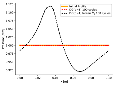
(b) Pressure after 100 cycles for $\mathrm{DG}(p=1)$ with total energy and frozen $\bar{C_{p}}$ formulation

Figure 5.4: Pressure for $\mathrm{DG}(p=1)$, $\mathrm{DG}(p=2)$, and $\mathrm{DG}(p=3)$ solutions after one cycle using $\mathrm{CFL}$ or 0.1 and $\mathrm{CFL}$ of 0.3 with frozen $\bar{C_{p}}$ and pressure after 100 cycles using total energy formulation and frozen $\bar{C_{p}}$ for $\mathrm{DG}(p=1)$.

5.1.2 Species Discontinuities and a Continuous Temperature Variation

A sinusoidal variation in temperature is introduced to the initial profile described in Section (5.1.1). The initial conditions are given as follows

$$v = 10\textrm{ m/s},$$

$$Y_{1} = \begin{cases}0&\text{if }0.025<x<0.075\\ 1&\text{otherwise}\end{cases},$$

$$Y_{2} = 1-Y_{1},$$

$$T = 350+50\sin\left(20\pi x\right)\textrm{ K},$$

$$p = 1\textrm{ atm}.$$

Figs. (5.5a), (5.5b), and (5.5c) show the species mass fractions for $\mathrm{DG}(p=1)$, $\mathrm{DG}(p=2)$, and $\mathrm{DG}(p=3)$ solutions after one cycle. Similar to the previous test case, the three solutions present numerical overshoots and mixing of the species mass fractions across the discontinuities. Here the left side discontinuity has larger overshoots in the higher temperature region as compared to the right hand side discontinuity.

Figure (5.6) shows the pressure for all three solutions using the total energy formulation and ratio of specific heats formulation with frozen $C_{p}$ and frozen $\bar{C_{p}}$ after one cycle. Fig. (5.6a) shows the large oscillations like the previous test case for the frozen $C_{p}$ formulation and smaller oscillations using the frozen $\bar{C_{p}}$ formulation. The oscillations caused by freezing $\bar{C_{p}}$ are reduced as the accuracy of the approximation is increased from $\mathrm{DG}(p=1)$ to $\mathrm{DG}(p=3)$. Again, the pressure for each solution using the total energy formulation maintains a flat pressure profile, even with a spatially varying temperature profile. This is expected as the temperature is continuous through the domain.

Figure (5.7) shows the computed temperature from solutions using the total energy formulation and the ratio of specific heats formulation with frozen $C_{p}$ and frozen $\bar{C_{p}}$ after one cycle. For the total energy and ratio of specific heats formulation with frozen $\bar{C}_{p}$ the temperature is within ${1}\mathrm{e}{-4}$ K of the analytical sinusoidal solution. The ratio of specific heats formulation with frozen $C_{p}$ is also shown and departs from the analytical result with the largest deviation of $5$ K in the higher temperature region

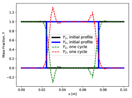
(a) $\mathrm{DG}\left(p=1\right)$ solution

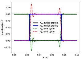
(b) $\mathrm{DG}\left(p=2\right)$ solution

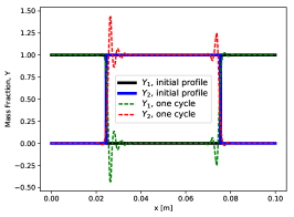
(c) $\mathrm{DG}\left(p=3\right)$ solution

Figure 5.5: Mass fractions for species 1 and 2 for one cycle through domain using the total energy formulation.

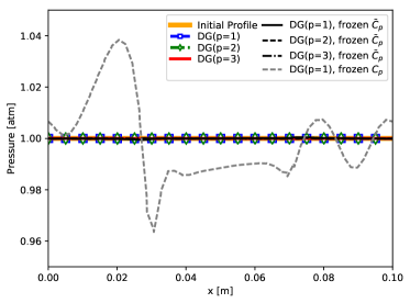
(a) Pressure

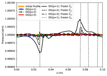
(b) Pressure zoomed view

Figure 5.6: Pressure for $\mathrm{DG}(p=1)$, $\mathrm{DG}(p=2)$, and $\mathrm{DG}(p=3)$ solutions after one cycle.

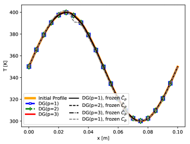
Figure 5.7: Temperature for $\mathrm{DG}(p=1)$, $\mathrm{DG}(p=2)$, and $\mathrm{DG}(p=3)$ solutions after one cycle.

5.1.3 Species Discontinuities with Temperature Discontinuities

The following test case uses the initial conditions described in Section 5.1.1, except the initial temperature profile is piecewise constant instead of constant. The initial conditions are given as follows

$$v = 10\textrm{ m/s},$$

$$Y_{1} = \begin{cases}0&\text{if }0.025<x<0.075\\ 1&\text{otherwise}\end{cases},$$

$$Y_{2} = 1-Y_{1},$$

$$T = \begin{cases}300\text{ K}&\text{if }0.025<x<0.075\\ 350\text{ K}&\text{otherwise}\end{cases},$$

$$p = 1\textrm{ atm}.$$

Figs. 5.8a, 5.8b, and 5.8c show the species mass fractions for $\mathrm{DG}(p=1)$, $\mathrm{DG}(p=2)$, and $\mathrm{DG}(p=3)$ solutions after one cycle. Similar to the previous test case, the three solutions present numerical overshoots and mixing of the species mass fractions across the discontinuities. Figs. 5.9a and 5.9b show the pressure and temperature, respectively, after one cycle for the total energy formulation and the ratio of specific heats formulation with frozen $\bar{C_{P}}$. The ratio of specific heats formulation with frozen $C_{p}$ simulation fails before one complete cycle. The solution corresponding to frozen $C_{p}$ is shown after 100 time steps. The pressure for each solution using the total energy formulation causes pressure oscillations that are an order of magnitude less than the frozen $\bar{C_{p}}$ simulations. The oscillations in the total energy formulation are expected based on the discussion in Section 3. Both the total energy formulation and the ratio of specific heats formulation with frozen $\bar{C_{p}}$ produce overshoots and undershoots at the temperature discontinuities. The temperature oscillations associated with the ratio of specific heats formulation with frozen $\bar{C_{p}}$ are larger than the oscillations corresponding to the total energy formulation.

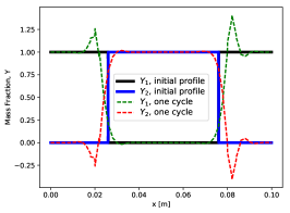
(a) $\mathrm{DG}\left(p=1\right)$ solution

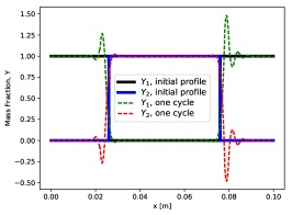
(b) $\mathrm{DG}\left(p=2\right)$ solution

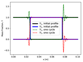
(c) $\mathrm{DG}\left(p=3\right)$ solution

Figure 5.8: Mass fractions for species 1 and 2 for one cycle through domain using the total energy formulation.

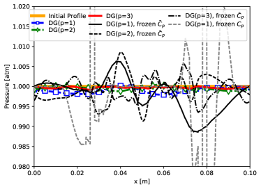
(a) Pressure solutions after one cycle.

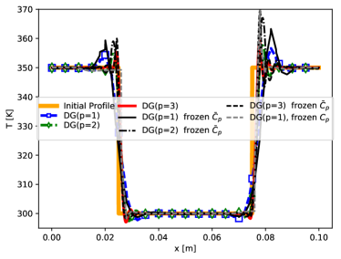
(b) Temperature solutions after one cycle.

Figure 5.9: Pressure and temperature for $\mathrm{DG}(p=1)$, $\mathrm{DG}(p=2)$, and $\mathrm{DG}(p=3)$ solutions after one cycle. The frozen $C_{p}$ solution at 100 steps is shown in grey.

Figs. 5.10a and 5.10b show the temperature and pressure solutions, respectively, for the total energy formulation and the ratio of specific heats formulation with frozen $\bar{C_{P}}$ after 100 cycles, i.e. $t=1$ s. The temperature profiles become more diffuse with the larger number of cycles (see Fig. 5.9b for the comparison of 1 cycle). The pressure oscillations for the total energy formulation cause the ambient pressure to fall below 1 atm. This departure from ambient was improved by increasing the approximation order from $\mathrm{DG}(p=1)$ to $\mathrm{DG}(p=3)$. The pressure oscillations for the 100 cycle solution using the frozen $\bar{C_{p}}$ formulation grow in time regardless of approximation order (see Fig. 5.9a for the one cycle solution for frozen $\bar{C_{P}}$). Furthermore, the frozen $\bar{C}_{p}$ formulation oscillations are an order of magnitude larger than the oscillations present in the total energy formulation.

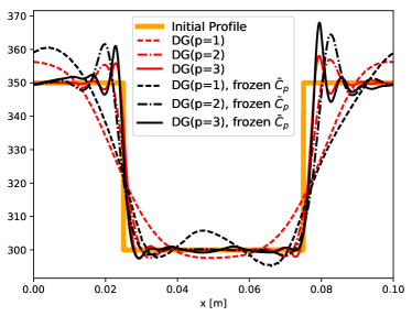
(a) Temperature solutions after 100 cycles.

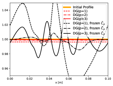
(b) Pressure solutions after 100 cycles.

Figure 5.10: Pressure and temperature for $\mathrm{DG}(p=1)$, $\mathrm{DG}(p=2)$, and $\mathrm{DG}(p=3)$ solutions after 100 cycles.

5.2 Continuous Simulations

5.2.1 Thermal Bubble

Here we present the one dimensional thermal bubble test case previously presented by [19]. For this test case, a periodic domain $50$ m domain, $(-25,25)$ m, with grid spacing, $h$, of 0.5 m is used with the following initial conditions

$$v = 1\textrm{ m/s},$$

$$Y_{H2} = \frac{1}{2}\left[1-\tanh\left(|x|-10\right)\right],$$

$$Y_{O_{2}} = 1-Y_{H_{2}},$$

$$T = 1200-900\tanh\left(|x|-10\right)\textrm{ K},$$

$$p = 1\textrm{ bar}.$$

The test case is run for 1 cycle, $t=50$ s, using $\mathrm{DG}(p=2)$ with $\mathrm{CFL}=0.1$ and the inviscid non-reacting formulation of Eqs. (2.1)- (2.3). No artificial viscosity or fail-safe limiting is used in this test case. The mesh resolution was too coarse to stably compute a $\mathrm{DG}(p=1)$ solution without limiting. Like the previous test cases, the analytical solution after one cycle is the same as the same as the initial profile. Figs. 5.11a and 5.11b show the results for pressure and temperature, respectively. The pressure is constant throughout for both the total energy formulation and the ratio of specific heats formulation with frozen $\bar{C_{p}}$ with variations on the order of ${1}\mathrm{e}{-5}\,$ atm. The pressure for the ratio of specific heats formulation with frozen $C_{p}$ fluctuates on the order of $10$% of the expected ambient pressure. Previous work reported that without the double flux method the pressure fluctuated throughout the solution by $3\%$ of the expected ambient pressure [19]. These issues do not occur in the solutions corresponding to the total energy formulation.

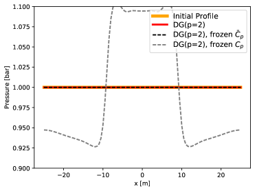
(a) Pressure solution after one cycle.

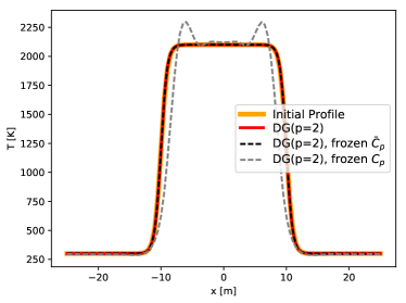
(b) Temperature solution after one cycle.

Figure 5.11: Thermal bubble simulation results corresponding to $\mathrm{DG}\left(p=2\right)$ after one cycle.

5.2.2 One-Dimensional Premixed Flame

We use the total energy formulation with detailed chemical kinetics and transport in the viscous, reacting formulation of Eqs. (2.1)- (2.3) to approximate the solution to a one-dimensional premixed flame using the Hydrogen-Air chemistry from [47]. The chosen domain is $6$ cm in length with $h={5}\mathrm{e}{-5}\,$m. We initialize the domain to an ambient pressure of $1$ bar, temperature of $300$ K, $X_{H_{2}}=0.188$, $X_{O_{2}}=0.170$, and $X_{N_{2}}=0.642$. A small section on the right hand side of the domain is initialized to the fully reacted state from Cantera’s homogeneous constant pressure reactor simulation [46].

The right hand side boundary is fixed to constant pressure with remaining variables interpolated from the interior state. The left hand side boundary is a characteristic wave boundary condition that allows any pressure waves caused by the initialization to exit the domain. The initialization contains a temperature and species discontinuity which gives rise to a pressure oscillation, which is supported by the analysis in Section 3. The initial pressure oscillations leave the system as the reaction front diffuses into the unreacted region, which eventually creates a stable propagating flame.

Figs. 5.12 and 5.13 show solutions for the $\mathrm{DG}\left(p=1\right)$ and $\mathrm{DG}\left(p=2\right)$ solutions, respectively. The temperature and species mass fraction profiles are compared to the Cantera flame solution with $h={1}\mathrm{e}{-5}\,$m and the profiles are shifted to have $T=400$ K at $x=0$. The $\mathrm{DG}\left(p=1\right)$ solutions reach the correct reacted state but cannot fully resolve the flame structures in the $-0.0005<x<0$ region. The $\mathrm{DG}\left(p=2\right)$ solution overcomes these errors and is in good agreement with the Cantera solution. Despite the under resolved profiles in the $\mathrm{DG}\left(p=1\right)$ solution, both solutions come close to the flame speed calculated in Cantera. The Cantera flame speed, given as the inflow velocity for the constant mass flow-rate, is 0.643 m/s. We considered the flame front in the unsteady $\mathrm{DG}\left(p=1\right)$ and $\mathrm{DG}\left(p=2\right)$ solutions to be the location corresponding to $T=1000$K. We tracked this location and computed a steady velocity of 0.641 m/s and 0.643 m/s for the $\mathrm{DG}\left(p=1\right)$ and $\mathrm{DG}\left(p=2\right)$ solutions, respectively.

Figs. 5.12d and 5.13d show the pressure through the entire computational domain for $\mathrm{DG}\left(p=1\right)$ and $\mathrm{DG}\left(p=2\right)$, respectively. For the $\mathrm{DG}\left(p=1\right)$ solution, there are small oscillations, on the order of $0.25$% of the ambient pressure. These oscillations are not present for the $\mathrm{DG}\left(p=2\right)$ solution, where only a slight variation is seen through the flame front but is constant on both sides of the flame within $0.1$% of the desired ambient pressure. The lack of pressure oscillations in the higher order solution indicate that the pressure oscillations in the $\mathrm{DG}\left(p=1\right)$ solution are due to the under-resolved flame and not related to the instabilities that would require stabilization.

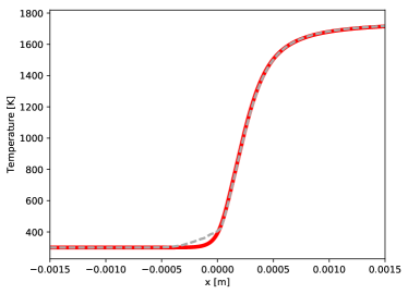
(a) Temperature profile, solid line is the Cantera solution on a uniform $h={1}\mathrm{e}{-5}\,$m grid, dashed grey line is the $\mathrm{DG}\left(p=1\right)$ solution. Results are shifted so that $T=400$ K at $x=0$ for both $\mathrm{DG}\left(p=1\right)$ and Cantera solutions.

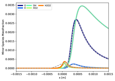
(b) Minor species profile, solid lines are Cantera solution on a uniform $h={1}\mathrm{e}{-5}\,$m grid, neighboring dashed grey lines are the$\mathrm{DG}\left(p=1\right)$ solution. Results are shifted so that $T=400$ K at $x=0$ for both $\mathrm{DG}\left(p=1\right)$ and Cantera solutions.

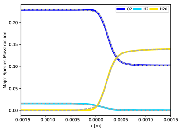
(c) Major species profile, solid lines are Cantera solution on a uniform $h={1}\mathrm{e}{-5}\,$m grid, neighboring dashed grey lines are the $\mathrm{DG}\left(p=1\right)$ solution. Results are shifted so that $T=400$ K at $x=0$ for both $\mathrm{DG}\left(p=1\right)$ and Cantera solutions.

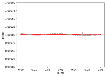
(d) Pressure profile for the entire simulation domain, solid line is constant 1 bar pressure, dashed grey line is $\mathrm{DG}\left(p=1\right)$ solution.

Figure 5.12: $\mathrm{DG}\left(p=1\right)$ flame solution

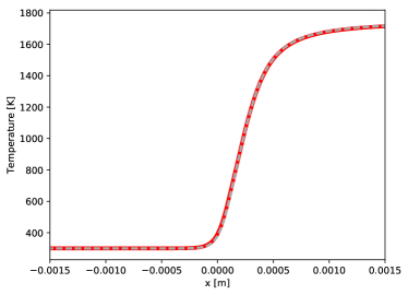
(a) Temperature profile, solid line is the Cantera solution on a uniform $h={1}\mathrm{e}{-5}\,$m grid, dashed grey line is the $\mathrm{DG}\left(p=2\right)$ solution. Results are shifted so that $T=400$ K at $x=0$ for both $\mathrm{DG}\left(p=2\right)$ and Cantera solutions.

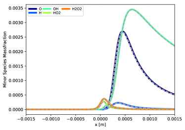
(b) Minor species profile, solid lines are Cantera solution on a uniform $h={1}\mathrm{e}{-5}\,$m grid, neighboring dashed grey lines are the $\mathrm{DG}\left(p=2\right)$ solution. Results are shifted so that $T=400$ K at $x=0$ for both $\mathrm{DG}\left(p=2\right)$ and Cantera solutions.

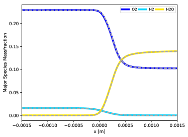
(c) Major species profile, solid lines are Cantera solution on a uniform $h={1}\mathrm{e}{-5}\,$m grid, neighboring dashed grey lines are the $\mathrm{DG}\left(p=2\right)$ solution. Results are shifted so that $T=400$ K at $x=0$ for both $\mathrm{DG}\left(p=2\right)$ and Cantera solutions.

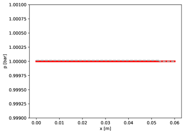
(d) Pressure profile for the entire simulation domain, solid line is constant 1 bar pressure, dashed grey line is $\mathrm{DG}\left(p=2\right)$ solution.

Figure 5.13: $\mathrm{DG}\left(p=2\right)$ flame solution

6 Conclusion

We have presented the total energy formulation and the ratio of specific heats formulation of the reacting Navier-Stokes equations and examined pressure oscillations for material interfaces with discontinuities in species and temperature. We derived that if the species internal energy is nonlinear with respect to temperature then pressure oscillations are only generated at material interfaces with discontinuities in both species and temperature. Pressure oscillations are not generated at a material interface with a species discontinuity if the temperature is continuous through the interface unless the thermodynamics are frozen during the temporal integration of the conserved state. The total energy formulation does not freeze the thermodynamics; instead a nonlinear relationship for temperature is solved which ensures consistency between the internal energy of the conserved state and the internal energy defined by a mixture averaged polynomial expression based on temperature. The converged temperature can then be use to evaluate other thermodynamic quantities so that they are consistent with the conserved state. As such, the total energy formulation can be integrated with a fully conservative method without generating pressure oscillations in regions of continuous pressure and temperature.

We presented several test cases to demonstrate the generation of unphysical pressure oscillations. We demonstrated that the pressure oscillations from the ratio of specific heats formulation with frozen $\bar{C}_{p}$ did not reach the magnitudes previously reported in literature  [23, 24, 18, 25, 19]. However, when it was assumed that the mean specific heat at constant pressure was the same as the NASA polynomial specific heat at constant pressure, $\bar{C_{p}}=C_{p}$, the oscillations did reach the same levels as previously reported, indicating that the severity of the pressure oscillations is dependent on the correct evaluation of thermodynamic quantities. Regardless, the pressure should be constant across the material interfaces and when $\bar{C}_{p}$ is frozen the magnitude of pressure oscillations will grow in time as the solution evolves. Additionally, the expected numerical pressure oscillations due to temperature discontinuities at material interfaces were less for the total energy formulation than for the ratio of specific heats formulation with frozen $\bar{C}_{p}$.

Previous work showed that advecting continuous species and temperature profiles caused unstable oscillations [18, 19]. We analyzed continuous profiles by presenting the thermal bubble test case for a multicomponent mixture of hydrogen and oxygen from  [19]. The total energy formulation solution for this test case did not generate pressure oscillations. The solutions reached the magnitudes of pressure oscillations found in the previous work only when the ratio of specific heats with frozen $C_{p}$ was used. When the ratio of specific heats with frozen $\bar{C}_{p}$ was used no pressure oscillations were generated due to the lack of numerical mixing for an advected continuous profile of species and temperature.

Finally, we presented the results for a fully reacting Navier-Stokes simulation of a continuous one-dimensional flame. The solution, computed using a fully conservative $\mathrm{DG}$ method without additional stabilization, compared well with the Cantera solution. Flame speeds for both the $\mathrm{DG}(p=1)$ and $\mathrm{DG}(p=2)$ solutions were consistent with the Cantera flame speed. Discrepancies between the Cantera solution and the $\mathrm{DG}(p=1)$ solution are not observed in the $\mathrm{DG}(p=2)$ solution, indicating the $\mathrm{DG}(p=2)$ solution better resolved the flame.

The total energy formulation does not require non-conservative methods or additional stabilization in smooth regions of the flow. This is an attractive feature since both non-conservative methods and artificial stabilization have associated inherent costs. Non-conservative methods often involve additional cell and face loops that increase the computational complexity. Additionally, artificial stabilization can prevent high order methods from achieving the formal order accuracy associated with the polynomial space of the approximate solution. We also demonstrated that the total energy formulation is equivalent to the ratio of specific heats formulation in non-reacting regions of the flow where thermodynamic quantities are not changing, which is a suitable alternative and may be convenient for methods that require the internal energy to be defined according to the ratio of specific heats, e.g., characteristic boundary conditions.

References

- [1] F. Bassi, S. Rebay, A high-order accurate discontinuous finite element method for the numerical solution of the compressible Navier–Stokes equations, Journal of Computational Physics 131 (2) (1997) 267–279.
- [2] F. Bassi, S. Rebay, High-order accurate discontinuous finite element solution of the 2D Euler equations, Journal of Computational Physics 138 (2) (1997) 251–285.
- [3] B. Cockburn, C.-W. Shu, The Runge–Kutta discontinuous Galerkin method for conservation laws V: multidimensional systems, Journal of Computational Physics 141 (2) (1998) 199–224.
- [4] B. Cockburn, G. Karniadakis, C.-W. Shu, The development of discontinuous Galerkin methods, in: Discontinuous Galerkin Methods, Springer, 2000, pp. 3–50.
- [5] D. Arnold, F. Brezzi, B. Cockburn, L. Marini, Unified analysis of discontinuous Galerkin methods for elliptic problems, SIAM Journal on Numerical Analysis 39 (5) (2002) 1749–1779.
- [6] R. Hartmann, P. Houston, Adaptive discontinuous Galerkin finite element methods for the compressible Euler equations, Journal of Computational Physics 183 (2) (2002) 508–532.
- [7] K. Fidkowski, T. Oliver, J. Lu, D. Darmofal, p-Multigrid solution of high-order discontinuous Galerkin discretizations of the compressible Navier–Stokes equations, Journal of Computational Physics 207 (1) (2005) 92–113.
- [8] H. Luo, J. Baum, R. Löhner, A p-multigrid discontinuous Galerkin method for the euler equations on unstructured grids, Journal of Computational Physics 211 (2) (2006) 767–783.
- [9] H. Luo, J. Baum, R. Löhner, A hermite weno-based limiter for discontinuous Galerkin method on unstructured grids, Journal of Computational Physics 225 (1) (2007) 686–713.
- [10] H. Luo, J. Baum, R. Löhner, A discontinuous Galerkin method based on a taylor basis for the compressible flows on arbitrary grids, Journal of Computational Physics 227 (20) (2008) 8875–8893.
- [11] P.-O. Persson, J. Peraire, Newton-GMRES preconditioning for discontinuous Galerkin discretizations of the Navier–Stokes equations, SIAM Journal on Scientific Computing 30 (6) (2008) 2709–2733.
- [12] R. Hartmann, T. Leicht, Higher order and adaptive DG methods for compressible flows, in: H. Deconinck (Ed.), VKI LS 2014-03: 37th Advanced VKI CFD Lecture Series: Recent developments in higher order methods and industrial application in aeronautics, Dec. 9-12, 2013, Von Karman Institute for Fluid Dynamics, Rhode Saint Genèse, Belgium, 2014.
- [13] J.-C. Lu, An a posteriori error control framework for adaptive precision optimization using discontinuous Galerkin finite element method, Ph.D. thesis, Massachusetts Institute of Technology (2005).
- [14] R. Hartmann, Adjoint consistency analysis of discontinuous Galerkin discretizations, SIAM Journal on Numerical Analysis 45 (6) (2007) 2671–2696.
- [15] R. Hartmann, T. Leicht, Generalized adjoint consistent treatment of wall boundary conditions for compressible flows, Journal of Computational Physics 300 (2015) 754–778.
- [16] A. Corrigan, A. Kercher, D. Kessler, A moving discontinuous Galerkin finite element method for flows with interfaces, Tech. Rep. NRL/MR/6040–17-9765, U.S. Naval Research Laboratory (December 2017).
- [17] A. Corrigan, A. Kercher, D. Kessler, A moving discontinuous Galerkin finite element method for flows with interfaces, International Journal for Numerical Methods in Fluids 89 (9) (2019) 362–406. doi:10.1002/fld.4697.
- [18] G. Billet, J. Ryan, A Runge–Kutta discontinuous Galerkin approach to solve reactive flows: The hyperbolic operator, Journal of Computational Physics 230 (4) (2011) 1064 – 1083. doi:https://doi.org/10.1016/j.jcp.2010.10.025.
- [19] Y. Lv, M. Ihme, Discontinuous Galerkin method for multicomponent chemically reacting flows and combustion, Journal of Computational Physics 270 (2014) 105 – 137. doi:https://doi.org/10.1016/j.jcp.2014.03.029.
- [20] R. Abgrall, Generalisation of the Roe scheme for the computation of mixture of perfect gases, La Recherche Aérospatiale 6 (1988) 31–43.
- [21] S. Karni, Multicomponent flow calculations by a consistent primitive algorithm, Journal of Computational Physics 112 (1) (1994) 31 – 43. doi:https://doi.org/10.1006/jcph.1994.1080.
- [22] R. Abgrall, How to prevent pressure oscillations in multicomponent flow calculations: A quasi conservative approach, Journal of Computational Physics 125 (1) (1996) 150 – 160. doi:https://doi.org/10.1006/jcph.1996.0085.
- [23] R. Abgrall, S. Karni, Computations of compressible multifluids, Journal of Computational Physics 169 (2) (2001) 594 – 623. doi:https://doi.org/10.1006/jcph.2000.6685.
- [24] G. Billet, R. Abgrall, An adaptive shock-capturing algorithm for solving unsteady reactive flows, Computers and Fluids 32 (10) (2003) 1473 – 1495. doi:https://doi.org/10.1016/S0045-7930(03)00004-5.
- [25] R. Houim, K. Kuo, A low-dissipation and time-accurate method for compressible multi-component flow with variable specific heat ratios, Journal of Computational Physics 230 (23) (2011) 8527 – 8553. doi:https://doi.org/10.1016/j.jcp.2011.07.031.
- [26] E. Johnsen, F. Ham, Preventing numerical errors generated by interface-capturing schemes in compressible multi-material flows, Journal of Computational Physics 231 (17) (2012) 5705 – 5717. doi:https://doi.org/10.1016/j.jcp.2012.04.048.
- [27] H. Terashima, M. Koshi, Approach for simulating gas liquid-like flows under supercritical pressures using a high-order central differencing scheme, Journal of Computational Physics 231 (20) (2012) 6907 – 6923. doi:https://doi.org/10.1016/j.jcp.2012.06.021.
- [28] Z. He, B. Tian, Y. Zhang, F. Gao, Characteristic-based and interface-sharpening algorithm for high-order simulations of immiscible compressible multi-material flows, Journal of Computational Physics 333 (2017) 247 – 268. doi:https://doi.org/10.1016/j.jcp.2016.12.035.
- [29] P. Ma, H. Wu, T. Jaravel, L. Bravo, M. Ihme, Large-eddy simulations of transcritical injection and auto-ignition using diffuse-interface method and finite-rate chemistry, Proceedings of the Combustion Institute 37 (3) (2019) 3303 – 3310. doi:https://doi.org/10.1016/j.proci.2018.05.063.
- [30] S. Arabi, J. Trépanier, R. Camarero, A simple extension of Roe’s scheme for multi-component real gas flows, Journal of Computational Physics 388 (2019) 178 – 194. doi:https://doi.org/10.1016/j.jcp.2019.03.007.
- [31] R. J. Kee, J. A. Miller, G. H. Evans, G. Dixon-Lewis, A computational model of the structure and extinction of strained, opposed flow, premixed methane-air flames, Symposium (International) on Combustion 22 (1) (1989) 1479 – 1494. doi:https://doi.org/10.1016/S0082-0784(89)80158-4.
- [32] C. R. Wilke, A viscosity equation for gas mixtures, J. Chem. Phys 18 (1950) 517–519. doi:10.1063/1.1747673.
- [33] S. Mathur, P. K. Tondon, S. C. Saxena, Thermal conductivity of binary, ternary and quaternary mixtures of rare gases, Molecular Physics 12 (1967) 569–579. doi:10.1080/00268976700100731.
- [34] T. J. Poinsot, S. K. Lele, Boundary conditions for direct simulations of compressible viscous flows, Journal of Computational Physics 101 (1) (1992) 104 – 129. doi:https://doi.org/10.1016/0021-9991(92)90046-2.
- [35] A. A. Madja, Compressible fluid flow and systems of conservation laws in several space variables / A. Majda, Vol. 4 of Applied mathematical sciences, Springer-Verlag, Springer-Verlag New York Inc, 1984.
- [36] P. Jenny, B. Mueller, H. Thomann, Correction of conservative euler solvers for gas mixtures, Journal of Computational Physics 132 (1) (1997) 91 – 107. doi:https://doi.org/10.1006/jcph.1996.5625.
- [37] M. J. Zahr, P.-O. Persson, An optimization-based approach for high-order accurate discretization of conservation laws with discontinuous solutions, ArXiv e-printsarXiv:1712.03445.
- [38] M. Zahr, P.-O. Persson, An optimization-based approach for high-order accurate discretization of conservation laws with discontinuous solutions, Journal of Computational Physics.
- [39] E. Toro, Riemann solvers and numerical methods for fluid dynamics: a practical introduction, Springer Science & Business Media, 2013.
- [40] F. Bassi, S. Rebay, An implicit high-order discontinuous Galerkin method for the steady state compressible navier-stokes equations, Computational fluid dynamics’98 (1998) 1226–1233.
- [41] F. Bassi, S. Rebay, Gmres discontinuous Galerkin solution of the compressible navier-stokes equations, in: Discontinuous Galerkin Methods, Springer, 2000, pp. 197–208.
- [42] F. Bassi, S. Rebay, Numerical evaluation of two discontinuous galerkin methods for the compressible navier–stokes equations, International journal for numerical methods in fluids 40 (1-2) (2002) 197–207.
- [43] S. Gottlieb, C. Shu, E. Tadmor, Strong stability-preserving high-order time discretization methods, SIAM review 43 (1) (2001) 89–112.
- [44] G. Strang, On the construction and comparison of difference schemes, SIAM Journal on Numerical Analysis 5 (3) (1968) 506–517.
- [45] B. J. McBride, M. J. Zehe, S. Gordon, NASA glenn coefficients for calculating thermodynamic properties of individual species.
-
[46]
D. G. Goodwin, H. K. Moffat, R. L. Speth,
Cantera: An object-oriented software toolkit
for chemical kinetics, thermodynamics, and transport processes, version
2.4.0 (2018).
doi:10.5281/zenodo.1174508.
URL http://www.cantera.org - [47] M. Ó Conaire, H. J. Curran, J. M. Simmie, W. J. Pitz, C. K. Westbrook, A comprehensive modeling study of hydrogen oxidation, International Journal of Chemical Kinetics 36 (11) (2004) 603–622. arXiv:https://onlinelibrary.wiley.com/doi/pdf/10.1002/kin.20036, doi:10.1002/kin.20036.