Scalar Field in Massive BTZ Black Hole and Entanglement Entropy

Abstract

In this paper, we investigate the quantum scalar fields in massive BTZ black hole background. We study the entropy of the system by evaluating the entanglement entropy with the use of discretized approach. Specifically, we fit the results with $\log$ -modified formula of the black hole entropy which is introduced by quantum correction. The coefficients of leading and sub-leading terms affected by the mass of graviton are numerically analyzed.

I Introduction

Black holes are solutions of Einstein equation in general gravitational theories, and the black hole is one of fascinating parts of our universe. Black holes are thermal systems because they were found to have temperature and entropy. The temperature of a black hole is proportional to the surface gravity at the event horizon. In the case of general relativity, the entropy, known as Bekenstein-Hawking entropy, is usually proportional to the area of the event horizon in the framework of black hole thermodynamics Israel:1967wq ; Unruh:1976db ; Hawking ; Shankaranarayanan:2000gb ; Angheben:2005rm ; Kerner:2006vu . However, when one considers quantum fields in the vicinity of black holes, the area law of entropy will get an additional quantum corrections. Till now, physicists have made plenty of attempts to disclose the microscopic essence of the black hole entropy and its connection with the area of event horizon. For instance, the authors of Gibbons ; Brown ; Hawking2 computed the entropy by evaluating the Euclidean action. The connecting between the entropy and instanton amplitude, which describes the pair production of charged black holes, can be seen in Garfinkle . The proposal that the entropy is the Noether charge of the bifurcate Killing horizon has been addressed in Wald ; Iyer . Later, the symmetry based approach to black hole entropy has been proposed, which connects the central charge of conformal field theory to the black hole entropyStrominger ; Carlip2 . This proposal of the central charge of the Virasoro algebra on the horizon has been generalized into the case of Witt algebraDreyer:2013noa , surface charge algebraBarnich:2007bf , Virasoro algebra null surfacesChakraborty:2016dwb and $2-$cocycles on the Lie algebraBarnich:2001jy and so on.

We know that the consideration of quantum mechanics gives rise to the thermal Hawking radiation, which does not carry information. One viewpoint is that the quantum gravity theory, such as string theory and loop quantum gravity, is called for to understand this information loss paradox. However, it was addressed in Mathur:2009hf that the interior of black holes has a ‘fuzzball’ structure. This gives a qualitative picture of how classical idea breaks down in black hole physics and the information paradox can be resolved. Especially, the authors somehow took care of both the near horizon behaviors and possible existence of singularity instead of focusing on one of them in the discussion. It is noticed that the microscopic derivation of black hole entropy was proposed with D-brane method in string theoryPolchinski and in brick wall modeltHooft . On the other hand, the entanglement entropy is a measure of the correlation between subsystems, which are separated by a boundary called the entangling surface. It is a measure of the information loss due to the division of the system, and so it depends on the geometry of the boundary Bombelli ; Srednicki . The entanglement entropy model, as one of the most attractive candidate of the black hole entropy, has been widely studiedFrolov ; Callan ; Kabat ; Holzhey ; Mukohyama ; Cadoni:2007vf ; Cadoni:2009tk ; Hung:2011ta .

In this paper, we aim to investigate the entropy of massive BTZ black holeHendi:2016pvx ; Chougule:2018cny via calculating its entanglement entropy by introducing a massless quantum scalar field. We shall apply the discretized approach to evaluate the entropy of the quantum scalar field in the spacetime by analyzing the similar harmonic oscillator, and we closely follow the procedure shown inBombelli ; Shiba:2013jja ; Shiba:2012np . We note that, similar studies on (rotating) BTZ black hole with massless or massive scalar field have been done in Singh:2011gd ; Sachan:2014hna , where the authors numerically analyzed the effect of angle momentum $(J)$ and mass of scalar field $(m_{s})$ on the coefficients in the entanglement entropy of BTZ black hole.

Here, we shall focus on the effect of the mass of graviton on the entanglement entropy in three dimensional massive black hole. As is known that black holes provide a particle environment for testing gravity and are incredibly important theoretical tools for exploring general gravity, and Schwarzschild black hole is the most general spherically symmetric vacuum solution. Massive gravity theory is one of the theories beyond Einstein’s gravity theory with massless graviton. In recent years, some cosmologists propose the idea of massive graviton to modify general relativity. One can also make contributions to explain the accelerated expansion of the universe without dark energyDAmico:2011eto . Early attempt of the construction in massive gravity has been established, such as linear theory of gravityFierz:1939ix and nonlinear model for massive gravity Vainshtein:1972sx . Recently, significant progress has been made in constructing massive gravity theories, which would avoid instability, see for example deRham:2010ik ; deRham:2010kj ; Hassan:2011hr ; Hassan:2011vm ; Hassan:2011tf ; Desai:2010ea ; Ludeling:2012cu . Various phenomenology of massive gravity has also been investigated widely. Moreover, the massive terms in the gravitational action break the diffeomorphism symmetry in the bulk, which corresponds to momentum dissipation in the dual boundary field theoryBlake:2013bqa .

This paper is organized as follows. We briefly review the massive BTZ black hole in three dimensional gravity theory in section II. We study the formula of the entanglement entropy of the massless quantum scalar field, and then evaluate the (sub-)leading coefficients of the entropy by fitting the numerical results in section III. Section IV contributes to our conclusions.

II Massive neutral BTZ black hole

We first briefly review the three dimensional Einstein-massive gravity with the action Hendi:2016pvx ; Chougule:2018cny

$$\mathscr{I}=-\frac{1}{16\pi}\int d^{3}x\sqrt{-g}\left[\mathscr{R}-2\Lambda+m^{2}\sum_{i}c_{i}\mathscr{U}_{i}(g,f)\right],$$ (1)

where $\mathscr{R}$ is the scalar curvature, $\Lambda=-1/L^{2}$ is the cosmological constant, and the last terms are Fierz-Pauli mass terms where $m$ denotes the mass of gravitonCreminelli:2005qk . Here, $c_{i}$ are constants and $\mathscr{U}_{i}$’s are symmetric polynomials of the eigenvalues of the $3\times 3$ matrix $\mathscr{K}_{\nu}^{\mu}\equiv\sqrt{g^{\mu\alpha}f_{\alpha\nu}}$. In this matrix, $g$ denotes the background metric, and the fixed rank$-2$ symmetric tensor $f$ is the reference metric which is inevitably included to construct the massive term of graviton in massive gravity and its form will be chosen later. As addressed in deRham:2010kj ; Hinterbichler:2011tt , $\mathscr{U}_{i}$ can be written as

$$\mathscr{U}_{1} = \left[\mathscr{K}\right],\;\;\;\;\;\mathscr{U}_{2}=\left[\mathscr{K}\right]^{2}-\left[\mathscr{K}^{2}\right],\;\;\;\;\;\mathscr{U}_{3}=\left[\mathscr{K}\right]^{3}-3\left[\mathscr{K}\right]\left[\mathscr{K}^{2}\right]+2\left[\mathscr{K}^{3}\right],$$ (2)

$$\mathscr{U}_{4}=\left[\mathscr{K}\right]^{4}-6\left[\mathscr{K}^{2}\right]\left[\mathscr{K}\right]^{2}+8\left[\mathscr{K}^{3}\right]\left[\mathscr{K}\right]+3\left[\mathscr{K}^{2}\right]^{2}-6\left[\mathscr{K}^{4}\right],\cdots$$

where the dots denote the higher order terms of $\mathscr{K}$. The square root in $\mathscr{K}$ denotes matrix square root, i.e, $(\sqrt{\mathscr{K}})^{\mu}_{\nu}(\sqrt{\mathscr{K}})^{\nu}_{\kappa}=\mathscr{K}^{\mu}_{~{}~{}\kappa}$, and the rectangular brackets denotes traces, i.e., $[\mathscr{K}]\equal\mathscr{K}^{\mu}_{\mu}$ and $[\mathscr{K}^{2}]\equal(\mathscr{K}^{2})^{\mu}_{~{}~{}\mu}$ with $(\mathscr{K}^{2})_{\mu\nu}\equal\mathscr{K}_{\mu\alpha}\mathscr{K}^{\alpha}_{~{}~{}\nu}$. We note that the study of ghost-free massive gravity can be seen in Hassan:2011hr ; Hassan:2011tf .

The action (1) gives us the Einstein equation

$$G_{\mu\nu}+\Lambda g_{\mu\nu}+m^{2}\chi_{\mu\nu}=0,$$ (3)

where the Einstein tensor $G_{\mu\nu}$ and massive term $\chi_{\mu\nu}$ are

$$G_{\mu\nu} = R_{\mu\nu}-\frac{1}{2}g_{\mu\nu}R,$$ (4)

$$\chi_{\mu\nu} = -\frac{c_{1}}{2}\left(\mathscr{U}_{1}g_{\mu\nu}-\mathscr{K}_{\mu\nu}\right)-\frac{c_{2}}{2}\left(\mathscr{U}_{2}g_{\mu\nu}-2\mathscr{U}_{1}\mathscr{K}_{\mu\nu}+2\mathscr{K}_{\mu\nu}^{2}\right)-\frac{c_{3}}{2}(\mathscr{U}_{3}g_{\mu\nu}-3\mathscr{U}_{2}\mathscr{K}_{\mu\nu}+$$ (5)

$$6\mathscr{U}_{1}\mathscr{K}_{\mu\nu}^{2}-6\mathscr{K}_{\mu\nu}^{3})-\frac{c_{4}}{2}(\mathscr{U}_{4}g_{\mu\nu}-4\mathscr{U}_{3}\mathscr{K}_{\mu\nu}+12\mathscr{U}_{2}\mathscr{K}_{\mu\nu}^{2}-24\mathscr{U}_{1}\mathscr{K}_{\mu\nu}^{3}+24\mathscr{K}_{\mu\nu}^{4}).$$

In order to solve the equation of motion, we take the ansatz of the metric as

$$ds^{2}=-f(r)dt^{2}+f^{-1}(r)dr^{2}+r^{2}d\varphi^{2},$$ (6)

where $f(r)$ is an arbitrary function of radial coordinate, and we will work with $L=1$ so that $\Lambda=-1$. Also following Vegh:2013sk , we choose the ansatz of the reference metric as

$$f_{\mu\nu}=\partial_{\mu}\phi^{a}\partial_{\nu}\phi^{b}\eta_{ab}=diag(0,0,c^{2}),$$ (7)

where $c$ is a positive constant, $\phi^{a}(x)$ is kind of coordinate transformation using $\eta_{ab}$ and different choices for the $\phi^{a}$ fields correspond to different gauges. Then with the metric ansatz (7), $\mathscr{U}_{i}$’s in (2) can be calculated asHassan:2011hr ; Cai:2014znn

$$\mathscr{U}_{1}=\frac{c}{r},\;\;\;\;\;\mathscr{U}_{2}=\mathscr{U}_{3}=\mathscr{U}_{4}=\cdots=0,$$ (8)

which means that in three dimensional case, the only contribution of massive terms comes from the term $\mathscr{U}_{1}$ in the action.

Subsequently, the independent Einstein equations are

$$rf^{\prime}(r)-2r^{2}-m^{2}cc_{1}r=0,$$ (9)

$$\frac{r^{2}}{2}f^{\prime\prime}(r)-r^{2}=0,$$ (10)

the solution to which is

$$f(r)=r^{2}-M+m^{2}cc_{1}r.$$ (11)

Here $M$ is an integration constant which is related to the total mass of the black hole. We note that in the absence of massive term with $m=0$, the solution recovers neutral BTZ black hole $f\left(r\right)=r^{2}-M$ without rotation.

Applying the standard method, we obtain the temperature of the black hole as

$$T=\frac{r_{+}}{2\pi}+\frac{m^{2}cc_{1}}{4\pi},$$ (12)

where $r_{+}$ is the event horizon satisfying $f(r_{+})=0$ and the Hawking entropy of the black hole is

$$S=\frac{\pi}{2}r_{+}.$$ (13)

For the convenience of further study, we shall do kind of transformation of the metric. The solutions to $f(r)=0$ are

$$r_{\pm}=\frac{-m^{2}cc_{1}\pm\sqrt{m^{4}c^{2}c_{1}^{2}+4M}}{2}.$$ (14)

Then, we introduce the proper length, $\rho$, by the coordinate transformation

$$r^{2}=r^{2}_{+}cosh^{2}\rho+r^{2}_{-}sinh^{2}\rho.$$ (15)

Subsequently, the metric of the black hole can be rewritten in terms of the proper length as

$$ds^{2}=-u^{2}dt^{2}+d\rho^{2}+\frac{[m^{2}+\sqrt{m^{4}+4(M+u^{2})}]^{2}}{4}d\varphi^{2}$$ (16)

where we have defined $u^{2}=r^{2}-M+m^{2}cc_{1}r$. In the following study, we will set $c=c_{1}=1$ without loss of generality.

III Entanglement entropy of massive BTZ black hole with scalar fields

III.1 Free massless scalar fields in massive BTZ black hole

The action of massless scalar field in the curved spacetime is

$$S_{scalar}=-\frac{1}{2}\int d^{3}x\sqrt{-g}g^{\mu\nu}\partial_{\mu}\Phi\partial_{\nu}\Phi.$$ (17)

In the background of massive BTZ black hole (16), considering the cylindrical symmetry of the system and the form of the scalar field

$$\Phi(t,\rho,\varphi)=\sum_{n}\Phi_{n}(t,\rho)e^{in\varphi},$$ (18)

we then further evaluate the action (17) as

$$S_{scalar}=-\frac{1}{2}\int d^{3}x \sum_{n}\Big{(}-\frac{m^{2}+\sqrt{m^{4}+4(M+u^{2})}}{2u}\dot{\Phi}_{n}^{2}+\frac{u[m^{2}+\sqrt{m^{4}+4(M+u^{2})}]}{2}(\partial_{\rho}\Phi_{n})^{2}$$ (19)

$$+n^{2}\frac{2u}{m^{2}+\sqrt{m^{4}+4(M+u^{2})}}\Phi_{n}^{2}\Big{)}=\int d^{3}x\sum_{n}\mathscr{L}_{n},$$

where we defined $\mathscr{L}_{n}$ as the Lagrangian density for the $n-$mode.

The conjugate momentum corresponding to $\Phi_{n}$ is given by

$$\pi_{n}=\frac{\delta\mathscr{L}_{n}}{\delta\dot{\Phi}_{n}}=\frac{2un^{2}}{m^{2}+\sqrt{m^{4}+4(M+u^{2})}}\Phi_{n}.$$ (20)

Therefore, the Hamiltonian density of the system is

$$H=\sum_{n}H_{n}=\sum_{n}\left(\frac{1}{2}\int d\rho\pi_{n}^{2}(\rho)+\frac{1}{2}\int d\rho d\rho^{\prime}\psi_{n}(\rho)V_{n}(\rho,\rho^{\prime})\psi_{n}(\rho^{\prime})\right)$$ (21)

where we introduced

$$\psi_{n}(t,\rho)=\sqrt{\frac{2u}{m^{2}+\sqrt{m^{4}+4(M+u^{2})}}}\Phi_{n}(t,\rho)$$ (22)

and

$$\psi_{n}(\rho)V_{n}(\rho,\rho^{\prime})\psi_{n}(\rho^{\prime})= \frac{u[m^{2}+\sqrt{m^{4}+4(M+u^{2})}]}{2}\Big{(}\partial_{\rho}(\sqrt{\frac{2u}{m^{2}+\sqrt{m^{4}+4(M+u^{2})}}})\psi_{n}\Big{)}^{2}$$ (23)

$$+\frac{2un^{2}}{(m^{2}+\sqrt{m^{4}+4(M+u^{2})})^{2}}\psi_{n}^{2}.$$

To proceed, we discretize the system for the convenience of computation via

$$\rho\rightarrow(A-1/2)a,\qquad\delta(\rho-\rho^{\prime})\rightarrow\delta_{AB}/a$$ (24)

where A,B=1,2 …N and ‘a’ is the UV cut-off length, so that $N\propto r_{+}/a$. We note that the continue limit recovers when $a\rightarrow 0$ and $N\rightarrow\infty$ as the size of system is fixed. Then, the Hamiltonian of the discretized system can be obtained by replacing

$$\psi_{n}(\rho)\rightarrow q^{A},\qquad\pi_{n}(\rho)\rightarrow p_{A}/a,\qquad V(\rho,\rho^{\prime})\rightarrow V_{AB}/a^{2}$$ (25)

in (21), the expression of which is then

$$H_{D}=\sum_{A,B=1}^{N}\left(\frac{1}{2a}\delta^{AB}p_{nA}p_{nB}+\frac{1}{2}V_{AB}^{n}q_{n}^{A}q_{n}^{B}\right).$$ (26)

Here, $V_{AB}^{n}$ is $N\times N$ matrix representation given as

$$(V_{AB}^{(n)})=\begin{bmatrix}\Sigma_{1}^{(n)}&\Delta_{1}&&&&\\ \Delta_{1}&\Sigma_{2}^{(n)}&\Delta_{2}&&&\\ &\ddots&\ddots&\ddots&&\\ &&\Delta_{A-1}&\Sigma_{A}^{(n)}&\Delta_{A}&&\\ &&&\ddots&\ddots&\ddots\\ \end{bmatrix},$$ (27)

with

$$\Sigma_{A}^{(n)}= \frac{2u_{A}}{m^{2}+\sqrt{m^{4}+4(M+u_{A}^{2})}}\Big{(}\frac{u_{A+1/2}[m^{2}+\sqrt{m^{4}+4(M+u_{A+1/2}^{2})}]}{2}$$ (28)

$$-\frac{u_{A-1/2}[m^{2}+\sqrt{m^{4}+4(M+u_{A-1/2}^{2})}]}{2}\Big{)}+n^{2}\frac{4u^{2}}{[m^{2}+\sqrt{m^{4}+4(M+u_{A}^{2})}]^{2}}$$

and

$$\Delta_{A}= -\frac{u_{A+1/2}[m^{2}+\sqrt{m^{4}+4(M+u_{A+1/2}^{2})}]}{2}\sqrt{\frac{2u_{A+1}}{m^{2}+\sqrt{m^{4}+4(M+u_{A}^{2})}}}$$ (29)

$$\times\sqrt{\frac{2u_{A}}{m^{2}+\sqrt{m^{4}+4(M+u_{A+1/2}^{2})}}}.$$

With the Hamiltonian (26)-(29) in hands, we are ready to apply the method shown in appendix A to evaluate the entanglement entropy of the system.

III.2 Numerical result of entanglement entropy

Following appendix A, the entanglement entropy of the above system is given byHuerta:2011qi

$$S=\lim\limits_{N\to\infty}S(n_{B},N)=S_{0}+2\sum_{n=1}^{\infty}S_{n},$$ (30)

where $S(n_{B},N)$ is the entanglement entropy of the total system $N$ with partition $n_{B}$; $S_{0}$ is the entanglement entropy of the system for $n=0$ and $S_{n}$ is the entropy of the subsystem for a given ‘n’, respectively.

We first study the entanglement entropy of the massive BTZ black hole at large N, which means that the change of result is not significant with increasing $N$. The numerical results are shown in table 1. We numerically calculate the $S_{n}$ for $n_{B}=10,50$ and $100$ at fixed $N=100$, and then we sum over ‘n’ as $S_{total}$. Specially, we show the results with different mass of graviton. The properties are summarized as follows. First, for fixed $N$ and $m$, larger $n_{B}$ corresponds to bigger $S_{n}$ and $S_{total}$. Second, with fixed $n_{B}$ and $m$, $S_{n}$ decreases for larger $n$ and finally it becomes slightly significant to the total entanglement entropy. These properties are specifically similar to those observed in Singh:2011gd . Third, with fixed $n_{B}$, $S_{total}$ is suppressed by stronger mass of graviton.

$n_{B}$	$S_{0}$			$S_{1}$			$S_{2}$			$\cdots$	$S_{total}=S$
	m=0	m=0.5	m=1	m=0	m=0.5	m=1	m=0	m=0.5	m=1	$\cdots$	m=0	m=0.5	m=1
$10$	0.98177	0.98190	0.98145	0.00732	0.00548	0.00331	0.00010	0.00046	0.00027	$\cdots$	0.99795	0.99399	0.98875
$50$	1.70383	1.70259	1.68877	0.25020	0.18895	0.15193	0.02178	0.01702	0.013599	$\cdots$	2.25842	2.12277	2.02639
$100$	2.39708	2.38928	2.33553	0.79353	0.72815	0.67098	0.14988	0.12739	0.156145	$\cdots$	4.35903	4.16412	4.06405

Table 1: The effect of mass of graviton on the entanglement entropy with fixed $N=100$ for different $n_{B}$.

Next, we numerically evaluate the entanglement entropy of the system with finite $N$. The entropy of the massive BTZ black hole is proportional to the area of the horizon as shown in (13), which we rewrite as $S=c_{1}r_{+}/a$ and $c_{1}$ is a constant while $a$ is the UV cut-off used to discretize the system. Considering the quantum effect, we should estimate the logarithmic correction to the black hole entropy as

$$S_{q}=c_{1}r_{+}/a+c_{2}\log(r_{+}/a)+c_{3}$$ (31)

where $c_{1},c_{2}$ and $c_{3}$ are all coefficients to be determined. We numerically calculate the entropy (30) and fit the results by (31) shown in figure 1. The fitted coefficients affected by the mass of graviton are shown in table 2. We see that the coefficient of the linear term, $c_{1}$, decreases as $m$, which is further fitted in figure 2. $c_{1}$ in the entanglement entropy is dependent of $m$, which is different from the constant in the Hawking entropy (13). This is reasonable because as we mentioned in footnote 3 that whether this entanglement entropy is exactly the black hole entropy is still an open question. It is worthwhile to point out that the entanglement entropy of massive black hole has also holographically studied inZeng:2015tfj ; Zhou:2019jlh via Ryu-Takayanagi formulaRyu:2006bv , and it was found that the massive of graviton would affect the entanglement entropy. So we argue that the massive term has explicit print on the entanglement entropy of black hole could be a universal property in massive gravity, even though the deep physics call for further study. Our result shows that the effect of mass of graviton on the entropy is similar to that of mass of scalar field observed in Sachan:2014hna . The sub-leading coefficient, $c_{2}$ is minus and also decreases as the mass increases while the fitting of $c_{3}$ is positive and bigger in massive BTZ black hole.

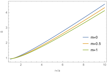
Figure 1: The entropy fitted by logarithmic correction (31) for different mass of graviton.

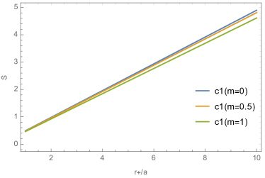
Figure 2: Linear fitting of the entropy for different $m$.

$c$	$m=0$	$m=0.5$	$m=1$
$c_{1}$	0.489594	0.480959	0.461284
$c_{2}$	-0.34156	-0.417998	-0.425697
$c_{3}$	0.452134	0.484263	0.504732

Table 2: Coefficients in (31) by fitting the entropy.

IV Conclusion and discussion

In this paper, we have evaluated the entanglement entropy of massive BTZ black hole by introducing a massless quantum scalar field with the use of the discretized approach. We found that in all cases, $S_{n}$ decreases as $n$ increases and finally it is not significant to the total entropy. Meanwhile, when we increase $n_{B}$, the entropy increases. The results are very similar to that found in Singh:2011gd . We also obtained that the larger mass of graviton would reduce the entropy. This means that comparing to the theory with massless graviton, the entropy computed by entanglement entropy in massive BTZ black hole is suppressed. Furthermore, we fitted the entropy by the quantum correction formula (31) and found the effect of massive term on the fitting coefficients. The linear coefficient decreases as $m$ increases, which is similar to the effect of the mass of scalar field obtained in Sachan:2014hna . The sub-leading coefficient of $\log$ term is suppressed while the constant $c_{3}$ is enhanced in massive BTZ black hole. Reminding that $m$ also explicitly affects the holographic entanglement entropy in massive gravity, we argued that it is universal that the massive term has print on the entanglement entropy of black hole in massive gravity, but the deep physics deserve further study.

As it was investigated in Singh:2014cca , it would be very interesting to extend our study by introducing Fermion field instead of scalar field into massive gravity and see the effect of massive term. We shall present the study elsewhere in the near future.

Appendix A Model of entanglement Entropy

In this appendix, we review the discretized method to calculate the entanglement entropy for scalar fieldsBombelli . Consider the system with coupled harmonic oscillators $q^{A},~{}(A=1,.......,N)$, the Hamiltonian of which is

$$H=\frac{1}{2a}\delta^{AB}p_{A}p_{B}+\frac{1}{2}V_{AB}q^{A}q^{B}.$$ (32)

Here $p^{A}$ and $p^{B}$ are canonical momentums conjugate to the $q^{A}$ and $q^{B}$, respectively, which are defined by the relation $p_{A}=a\,\delta_{AB}\,\dot{q}^{B}$ with the Kronecker delta $\delta_{AB}$. $V_{AB}$ is real, symmetric, positive definite matrix and “a” is fundamental length characterizing the system. By defining a symmetric, positive definite matrix via $V_{AB}=W_{AC}W^{C}_{B}$, one can rewrite the total Hamiltonian as,

$$H=\frac{1}{2a}\delta^{AB}\left(p_{A}+iW_{AC}q^{C}\right)\left(p_{B}-iW_{BD}q^{D}\right)+\frac{1}{2a}\,\mathrm{Tr}~{}W.$$ (33)

The new operators $(p_{A}+iW_{AC}q^{C})$ and $(p_{B}-iW_{BD}q^{D})$ are the annihilation and creation operators respectively, which are similar to those of harmonic oscillator problem and they obey similar commutation relation, $[a_{A},a_{B}^{\dagger}]=2W_{AB}$.

In the harmonic oscillator system, then the ground state $\psi_{0}$ satisfies

$$(p_{A}-iW_{AC}q^{C})|\psi_{0}>=0$$ (34)

and the solution is Bombelli

$$\psi_{0}(\{q^{C}\}) = <\{q^{C}\}|\psi_{0}>=\left[\det\frac{W}{\pi}\right]^{1/4}\mathrm{exp}\left[-\frac{1}{2}W_{AB}\,q^{A}\,q^{B}\right].$$ (35)

Therefore, the density matrix of the ground state is

$$\rho\left(\{q^{A}\},\{q^{\prime B}\}\right) = <\{q^{A}\}|0><0|\{q^{\prime B}\}>=\left[\mathrm{det}\frac{W}{\pi}\right]^{1/2}\mathrm{exp}\left[-\frac{1}{2}W_{AB}\,(q^{A}\,q^{B}+q^{\prime A}\,q^{\prime B})\right].$$ (36)

We divide ${q^{A}}$ into two subsystems, ${\{q^{a}\}}$ $(a=1,2,.......n_{B})$ and $\{q^{\alpha}\}$ $(\alpha=n_{B}+1,n_{B}+2,.......N)$. Then the reduced density matrix of one subsystem is obtained by tracing the degrees of freedom of the other subsystem as

$$\rho\Big{(}\{q^{\prime a}\},\{q^{\prime b}\}\Big{)}=\int\prod_{\alpha}dq^{\alpha}\rho\,\Big{(}\{q^{a},q^{\alpha}\},\{q^{\prime b},q^{\alpha}\}\Big{)}.$$ (37)

Thus, the matrix $W$ can split into four blocks as,

$$(W)_{AB}=\left(\begin{array}[]{ccc}A_{ab}&B_{a\beta}\\ B^{T}_{\alpha b}&D_{\alpha\beta}\end{array}\right).$$

Consequently, the reduced density matrix is rewritten as,

$$\rho_{red}(\{q^{a}\},\{q^{\prime b}\})=\left[\mathrm{det}\frac{M}{\pi}\right]^{1/2}e^{-\frac{1}{2}M_{ab}(q^{a}q^{b}+q^{\prime a}q^{\prime b})}e^{-\frac{1}{4}N_{ab}(q-q^{\prime})^{a}(q-q^{\prime})^{b}}$$ (38)

where

$$M_{ab}=(A-BD^{-1}B^{T})_{ab}\qquad\text{and}\qquad N_{ab}=(B^{T}A^{-1}B)_{ab}.$$ (39)

The system can be diagonalized by the unitary matrix $U$ and the transformations

$$q^{a}\rightarrow\tilde{q}^{a}=(UM^{1/2})^{a}_{b}q^{b}.$$ (40)

Thus, the density matrix can be further reduced into Bombelli ,

$$\rho_{red}(\{q^{a}\},\{q^{b}\}) =\Pi_{n}\left[\pi^{-1/2}\exp\left(-\frac{1}{2}(q_{n}q^{n}+q^{\prime}_{n}q^{\prime n}\right.\right.-\left.\left.\frac{1}{4}\lambda_{i}(q-q^{\prime})_{n}(q-q^{\prime})^{n})\right)\right],$$ (41)

where $\lambda_{i}$ are the eigenvalues of the matrix $\Lambda^{a}_{b}=(M^{-1})^{ac}N_{cb}$. Thus, the entanglement entropy of the system can be calculated by the relation (30) with

$$S_{n}=-\sum_{i}\ln(\lambda_{i}^{1/2}/2)+(1+\lambda_{i})^{1/2}\ln(1+\lambda_{i}^{-1}+\lambda_{i}^{-1/2}).$$ (42)

- (1) W. Israel, Phys. Rev. 164, 1776 (1967).
- (2) W. G. Unruh, Phys. Rev. D 14, 870 (1976).
- (3) S. W. Hawking, Phy. Rev. D 13, 191 (1976).
- (4) S. Shankaranarayanan, K. Srinivasan and T. Padmanabhan, Mod. Phys. Lett. A 16, 571 (2001).
- (5) M. Angheben, M. Nadalini, L. Vanzo and S. Zerbini, JHEP 0505, 014 (2005).
- (6) R. Kerner and R. B. Mann, Phys. Rev. D 73, 104010 (2006).
- (7) T. Clunan, S. F. Ross and D. J. Smith, Class. Quant. Grav. 21 (2004) 3447 [gr-qc/0402044].
- (8) T. Jacobson and R. C. Myers, Phys. Rev. Lett. 70, 3684 (1993) [hep-th/9305016].
- (9) S. Chakraborty, JHEP 1508 (2015) 029 [arXiv:1505.07272 [gr-qc]].
- (10) G. W. Gibbons and S. W. Hawking, Phys. Rev. D 15, 2752 (1977).
- (11) J. D. Brown and J. W. York, Jr., Phys. Rev. D 47, 1420 (1993) [gr-qc/9209014].
- (12) S. W. Hawking and C. J. Hunter, Phys. Rev. D 59, 044025 (1999) [hep-th/9808085].
- (13) D. Garfinkle, S. B. Giddings and A. Strominger, Phys. Rev. D 49, 958 (1994) [gr-qc/9306023].
- (14) R. M. Wald, Phys. Rev. D 48, no. 8, R3427 (1993) [gr-qc/9307038].
- (15) V. Iyer and R. M. Wald, Phys. Rev. D 50, 846 (1994) [gr-qc/9403028].
- (16) A. Strominger, JHEP 9802, 009 (1998) [hep-th/9712251].
- (17) S. Carlip, Phys. Rev. Lett. 82, 2828 (1999) [hep-th/9812013].
- (18) O. Dreyer, A. Ghosh and A. Ghosh, Phys. Rev. D 89 (2014) no.2, 024035 [arXiv:1306.5063 [gr-qc]].
- (19) G. Barnich and G. Compere, J. Math. Phys. 49 (2008) 042901 [arXiv:0708.2378 [gr-qc]].
- (20) S. Chakraborty, S. Bhattacharya and T. Padmanabhan, Phys. Lett. B 763 (2016) 347 [arXiv:1605.06988 [gr-qc]].
- (21) G. Barnich and F. Brandt, Nucl. Phys. B 633 (2002) 3 [hep-th/0111246].
- (22) S. D. Mathur, Class. Quant. Grav. 26 (2009) 224001 [arXiv:0909.1038 [hep-th]].
- (23) J. Polchinski, S. Chaudhuri and C. V. Johnson, hep-th/9602052; A. Strominger and C. Vafa, Phys. Lett. B 379, 99 (1996) [hep-th/9601029]; J. M. Maldacena, [hep-th/9607235].
- (24) G. ¡¯tHooft, Nucl. Phys. B 256, 727 (1985).
- (25) L. Bombelli, R. K. Koul, J. Lee and R. D. Sorkin, Phys. Rev. D 34, 373 (1986).
- (26) M. Srednicki, Phys. Rev. Lett. 71, 666 (1993) [hep-th/9303048].
- (27) V. P. Frolov and I. Novikov, Phys. Rev. D 48, 4545 (1993) [gr-qc/9309001].
- (28) C. G. Callan, Jr. and F. Wilczek, Phys. Lett. B 333, 55 (1994) [hep-th/9401072].
- (29) D. N. Kabat and M. J. Strassler, Phys. Lett. B 329, 46 (1994) [hep-th/9401125].
- (30) C. Holzhey, F. Larsen and F. Wilczek, Nucl. Phys. B 424, 443 (1994) [hep-th/9403108].
- (31) S. Mukohyama, M. Seriu and H. Kodama, Phys. Rev. D 55, 7666 (1997);Phys. Rev. D 58, 064001 (1998) [gr-qc/9701059].
- (32) M. Cadoni, Phys. Lett. B 653 (2007) 434.
- (33) M. Cadoni and M. Melis, Found. Phys. 40 (2010) 638; Entropy 2010, 12, 2244-2267.
- (34) L. -Y. Hung, R. C. Myers and M. Smolkin, JHEP 1108 (2011) 039, [arXiv:1105.6055 [hep-th]].
- (35) S. H. Hendi, B. Eslam Panah and S. Panahiyan, JHEP 1605, 029 (2016) [arXiv:1604.00370 [hep-th]].
- (36) S. Chougule, S. Dey, B. Pourhassan and M. Faizal, Eur. Phys. J. C 78 (2018) no.8, 685 [arXiv:1809.00868 [gr-qc]].
- (37) N. Shiba and T. Takayanagi, JHEP 1402 (2014) 033 [arXiv:1311.1643 [hep-th]].
- (38) N. Shiba, JHEP 1207 (2012) 100 [arXiv:1201.4865 [hep-th]].
- (39) D. V. Singh and S. Siwach, Class. Quant. Grav. 30, 235034 (2013) [arXiv:1106.1005 [hep-th]].
- (40) D. V. Singh and S. Sachan, Int. J. Mod. Phys. D 26, no. 04, 1750038 (2016) [arXiv:1412.7170 [hep-th]].
- (41) G. D’Amico, C. de Rham, S. Dubovsky, G. Gabadadze, D. Pirtskhalava and A. J. Tolley, Phys. Rev. D 84, 124046 (2011) [arXiv:1108.5231 [hep-th]].
- (42) M. Fierz and W. Pauli, Proc. Roy. Soc. Lond. A 173, 211 (1939).
- (43) A. I. Vainshtein, Phys. Lett. 39B, 393 (1972).
- (44) C. de Rham and G. Gabadadze, Phys. Rev. D 82, 044020 (2010) [arXiv:1007.0443 [hep-th]].
- (45) C. de Rham, G. Gabadadze and A. J. Tolley, Phys. Rev. Lett. 106, 231101 (2011) [arXiv:1011.1232 [hep-th]].
- (46) S. F. Hassan and R. A. Rosen, Phys. Rev. Lett. 108, 041101 (2012) [arXiv:1106.3344 [hep-th]].
- (47) S. F. Hassan and R. A. Rosen, JHEP 1107, 009 (2011) [arXiv:1103.6055 [hep-th]].
- (48) S. F. Hassan, R. A. Rosen and A. Schmidt-May, JHEP 1202, 026 (2012) [arXiv:1109.3230 [hep-th]].
- (49) K. M. Desai et al., Astron. J. 140, 584 (2010) [arXiv:1006.3344 [astro-ph.GA]].
- (50) C. Ludeling, F. Ruehle and C. Wieck, Phys. Rev. D 85, 106010 (2012) [arXiv:1203.5789 [hep-th]].
- (51) M. Blake and D. Tong, Phys. Rev. D 88, no. 10, 106004 (2013)
- (52) P. Creminelli, A. Nicolis, M. Papucci and E. Trincherini, JHEP 0509 (2005) 003 [hep-th/0505147].
- (53) K. Hinterbichler, Rev. Mod. Phys. 84 (2012) 671 doi:10.1103/RevModPhys.84.671 [arXiv:1105.3735 [hep-th]].
- (54) D. Vegh, arXiv:1301.0537 [hep-th].
- (55) R. G. Cai, Y. P. Hu, Q. Y. Pan and Y. L. Zhang, Phys. Rev. D 91, no. 2, 024032 (2015) [arXiv:1409.2369 [hep-th]].
- (56) M. Huerta, Phys. Lett. B 710, 691 (2012) [arXiv:1112.1277 [hep-th]].
- (57) X. X. Zeng, H. Zhang and L. F. Li, Phys. Lett. B 756 (2016) 170 [arXiv:1511.00383 [gr-qc]].
- (58) Y. T. Zhou, M. Ghodrati, X. M. Kuang and J. P. Wu, Phys. Rev. D 100 (2019) no.6, 066003 [arXiv:1907.08453 [hep-th]].
- (59) S. Ryu and T. Takayanagi, Phys. Rev. Lett. 96 (2006) 181602 [hep-th/0603001].
- (60) D. V. Singh and S. Siwach, Adv. High Energy Phys. 2015, 528762 (2015) [arXiv:1406.3799 [hep-th]].