Exploring the Asymmetry of the Solar Corona Electron Density
with Very Long Baseline Interferometry

Abstract

The Sun’s corona has interested researchers for multiple reasons, including the search for solution for the famous coronal heating problem and a purely practical consideration of predicting geomagnetic storms on Earth. There exist numerous different theories regarding the solar corona; therefore, it is important to be able to perform comparative analysis and validation of those theories. One way that could help us move towards the answers to those problems is the search for observational methods that could obtain information about the physical properties of the solar corona and provide means for comparing different solar corona models.

In this work we present evidence that VLBI observations are, in certain conditions, sensitive to the electron density of the solar corona and are able to distinguish between different electron density models, which makes the technique of VLBI valuable for solar corona investigations. Recent works on the subject used a symmetric power-law model of the electron density in solar plasma; in this work, an improvement is proposed based on a 3D numerical model.

a

This is the version of the article accepted for publication including all changes made as a result of the peer review process, and which may also include the addition to the article by IOP Publishing of a header, an article ID, a cover sheet and/or an ‘Accepted Manuscript’ watermark, but excluding any other editing, typesetting or other changes made by IOP Publishing and/or its licensors.

1 Introduction

Since the discovery of the solar corona in the 19th century to this day, the physical processes happening inside it are not completely understood. In particular (see e.g. Cranmer, 2002), the cause of heat of the $10^{6}$ K of the corona and acceleration of the solar wind is not known with certainty. While many theories were proposed, and more continue to appear and compete with each other, observational data is needed to eliminate wrong assumptions. There are very useful and important observations of solar corona by spacecraft, like STEREO (Harrison et al., 2008); moreover, in situ measurements of the solar corona by Parker Solar Probe (Bale et al., 2016) are expected soon. However, it is also possible to perform high-quality measurements of the solar corona from Earth; that is, to measure one particular property of the corona—the electron density—along a ray path.

The idea of determining electron densities in space plasmas by means of measuring group time-delays of radio signals traveling between a transmitter located on Earth and an interplanetary spacecraft was formulated at the times of the first spacecraft launches (Kelso, 1959). Since then, numerous works regarding the use of radio measurements for determining the electron density in one particular space plasma, the solar corona, have been published. Those works were traditionally based on analysis of single- and dual-frequency time-delay observations of spacecrafts orbiting Venus and Mars. An overview of some of such works is given by Bird & Edenhofer (1990); Bird et al. (2012).

Besides spacecraft tracking, a technique that measures time delays of radio signals and could, in theory, determine the solar corona’s electron density, is very long baseline interferometry (VLBI). The quantity measured by VLBI is the difference in arrival times of a signal from an extragalactic radio source received at two radio telescopes (Schuh & Behrend, 2012). As the spatial distribution of the electron density of the solar corona is clearly not uniform, the dispersive delays accumulated by radio signals passing through different regions of the corona would also be different, and measuring these differences should allow for reconstruction of the electron density.

Though yet not particularly common, the idea of utilizing VLBI for solar corona electron density measurements has been adopted in several recent works. Specifically, the parameters of a simple power-law model for the electron density were estimated using data of multiple VLBI sessions from 2011–2012 (Soja et al., 2014, 2015) and one VLBI session from 2017 (Soja et al., 2018). Results of these works will be discussed in more detail in further sections of this paper.

2 Electron density models

2.1 Power-law model

Typically, when it comes to measuring the electron density in the solar corona by means of radio sounding, most works tend to adopt a simple symmetric power-law model of the electron density

$$N_{\mathrm{e}}(r)=\frac{N_{0}}{r^{\alpha}},$$ (1)

where $N_{0}=N_{\mathrm{e}}(R_{\odot})$ is an estimated parameter with the physical meaning of electron number density at the surface of the Sun and $\alpha$ is either estimated or set to be approximately equal to 2.

A simplistic physical perspective gives a rough estimate of what the value of $\alpha$ could or should be. Suppose that the solar corona has a stationary electron density distribution $N_{\mathrm{e}}(r)$ and that there is a radial outflow of the electrons with non-constant drift velocity $v(r)$. Then the continuity equation must hold (Parker, 1958; Meyer-Vernet, 2007):

$$\frac{\partial N_{\mathrm{e}}(r)}{\partial t}+\nabla\cdot\mathbf{j}(r)=0,$$ (2)

where $\mathbf{j}(r)=\hat{\mathbf{r}}\,v(r)N_{\mathrm{e}}(r)$ is the particle flux. The density distribution is said to be stationary, therefore, $\partial N_{\mathrm{e}}/\partial t=0$ and

$$\frac{\partial}{\partial r}\left(r^{2}v(r)N_{\mathrm{e}}(r)\right)=0,$$ (3)

$$r^{2}v(r)N_{\mathrm{e}}(r)=\mathrm{const}.$$ (4)

Hence, if the electrons drift away with constant velocity, the electron density decreases proportionally to $1/r^{2}$. The density should fall faster than $1/r^{2}$ if the electrons are accelerating and slower if the electrons are decelerating. As some works suggest (Pierrard et al., 1999; Cranmer et al., 2007), electrons might indeed be accelerating on heliospheric distances up to roughly $40R_{\odot}$, and in that case fitting the power-law density model to observational data should naturally lead to powers greater than 2.

In fact, values of $N_{0}$ and $\alpha$ in eq. 1 vary significantly between different works (Berman, 1977), which is usually attributed to variances in solar activity. Moreover, they vary even between different sides of the Sun during a single experiment with a single spacecraft (Anderson et al., 1987), which raises concern about the validity of symmetric models.

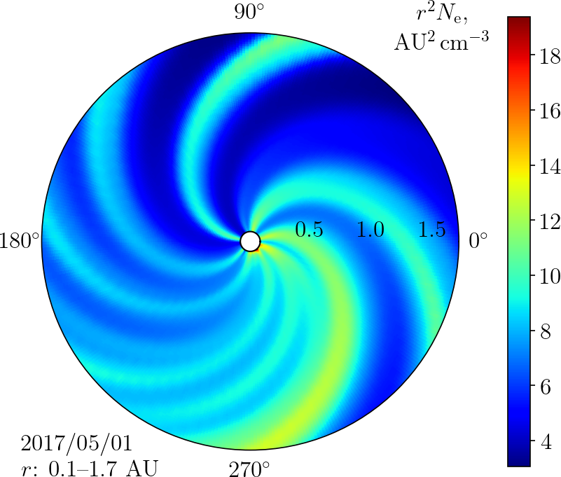
Figure 1: Solar wind electron density from the ENLIL model. The data is plotted in the plane with latitude of 0° in HEEQ coordinate system (see Thompson, 2006).

2.2 Three-dimensional MHD models

A compelling alternative to symmetric power-law models is offered by a class of numerical three-dimensional magnetohydrodynamic (MHD) models. Unlike power-law models, which, at any given time, are but an approximation for real electron density distributions occurring in the solar corona, 3D MHD models aim to provide real-time spatial distributions of electron density, velocity and other parameters of the solar plasma. That is achieved by numerically solving a set of non-linear differential equations called MHD equations with boundary condition for the magnetic field on solar surface given by synoptic magnetograms.

Since MHD models do not impose any restrictions on the solution, which symmetric power-law models obviously do in multiple ways, and also rely on physical principles and observational data, they should, in principle, lead to substantially more accurate results than the power law. An illustration to this claim is given in Figure 1, which shows an electron density distribution given by a 3D MHD model and suggests that the solar corona is highly non-stationary and non-symmetric and that symmetric models of any kind, let alone the power law, are not sophisticated enough to accurately describe it.

Examples of MHD models are the ENLIL solar wind model (Taktakishvili et al., 2011), which provides solutions for heliospheric distances greater than 0.1 AU ($21.5R_{\odot}$), and Alfvén Wave Solar Model (AWSoM-R, Sokolov et al., 2013; van der Holst et al., 2014), implemented on top of the Space Weather Modeling Framework (SWMF, Tóth et al., 2012), which simulates both inner and outer heliosphere on heliospheric distances from $1.15R_{\odot}$ to $250R_{\odot}$. Also available are results of validation of the AWSoM model against observational data. For instance, van der Holst et al. (2014) have compared simulated multi-wavelength extreme ultraviolet (EUV) images with observations from Solar Terrestrial Relations Observatory (STEREO) and Solar Dynamics Observatory (SDO); Oran et al. (2013) have compared AWSoM model results with remote observations in the extreme-ultraviolet and X-ray ranges from STEREO, Solar and Heliospheric Observatory, and Hinode spacecraft and with in situ measurements by Ulysses; Moschou et al. (2018) have compared predictions of the bremsstrahlung radio emission from the AWSoM model with observations of the Sun at MHz and GHz frequencies. All the studies have found the AWSoM model predictions to be in agreement with observational data.

Simulation data for ENLIL and AWSoM models is provided by request on the CCMC website.

2.3 Overview

Generally speaking, the power-law model (i.e. $1/r^{2}$) is merely a typical average radial profile of the electron density. While it could, in theory, agree with some kind of observations on a long-term scale (e.g. spacecraft ranging observations during multiple months), it would be quite unreasonable to assume that it would work well with instantaneous measures like VLBI. Electron density at any fixed point in time and space cannot possibly be accurately predicted by an average dependency. Therefore, instantaneous observations should be in significantly better agreement with non-symmetric time-dependent models like ENLIL and AWSoM than with the power law.

3 Radio wave propagation in the corona

3.1 Refractive index

The dispersion relation for plasma is (Goldston & Rutherford, 1995)

$$\omega^{2}=\omega_{\mathrm{p}}^{2}+k^{2}c^{2},$$ (5)

where $\omega$ and $k$ are the wave’s angular frequency and wavevector, $c$ is the speed of light, and $\omega_{\mathrm{p}}$ is the plasma frequency given by

$$\omega_{\mathrm{p}}=\sqrt{\frac{N_{\mathrm{e}}\,e^{2}}{m_{\mathrm{e}}\epsilon_{0}}},$$ (6)

where $N_{\mathrm{e}}(\mathbf{r})$ is the electron number density, $e$ and $m_{\mathrm{e}}$ are the electron’s charge and mass, and $\epsilon_{0}$ is the electric constant. The group velocity and the group refractive index are then

$$v_{\mathrm{gr}} =\frac{\partial\omega}{\partial k}=c\,\sqrt{1-\frac{\omega_{\mathrm{p}}^{2}}{\omega^{2}}},$$ (7)

$$n_{\mathrm{gr}} =\frac{c}{v_{\mathrm{gr}}}=\frac{1}{\sqrt{1-\omega_{\mathrm{p}}^{2}/\omega^{2}}}.$$ (8)

Given that the frequency of VLBI X-band is about $10^{9}$ Hz and that for heliospheric distances of $4R_{\odot}$, which is closer to the Sun than observations by VLBI have ever been performed, the electron density is about $10^{10}\ \mathrm{m}^{-3}$, the term $\omega_{\mathrm{p}}^{2}/\omega^{2}$ is not greater than $10^{-7}$. Therefore, as $\omega_{\mathrm{p}}^{2}/\omega^{2}\ll 1$, we can expand $n_{\mathrm{gr}}$ to first order of $\omega_{\mathrm{p}}^{2}/\omega^{2}$ and get

$$n_{\mathrm{gr}}\approx 1+\frac{\omega_{\mathrm{p}}^{2}}{2\,\omega^{2}}.$$ (9)

Rewriting the above in terms of critical plasma density

$$N_{\mathrm{crit}}(\omega)=\frac{m_{\mathrm{e}}\,\epsilon_{0}\,\omega^{2}}{e^{2}}\approx 1.24\cdot 10^{-2}\ \frac{\mathrm{s}^{2}}{\mathrm{m}^{3}}\cdot f^{2}$$ (10)

and introducing spatial variability in the electron density, finally,

$$n_{\mathrm{gr}}(\mathbf{r})\approx 1+\frac{N_{\mathrm{e}}(\mathbf{r})}{2\,N_{\mathrm{crit}}(\omega)}\approx 1+\frac{40.3\ \mathrm{m}^{3}\,\mathrm{s}^{-2}}{f^{2}}N_{\mathrm{e}}(\mathbf{r}),$$ (11)

where $f$ is the wave’s frequency in Hz.

3.2 Fermat’s principle

According to the Fermat’s principle, the path taken between two points by a photon is the path with the least optical path length (OPL)

$$S=\int_{\mathbf{r}_{a}}^{\mathbf{r}_{b}}n\,\mathrm{d}s\ \rightarrow\ \mathrm{min},$$ (12)

where $n$ is the index of refraction, and the integral is taken along the ray trajectory.

The above means that, in order to calculate the OPL between two points in the solar corona, one has to solve the variational problem (12), taking into account the path curvature introduced by the Sun’s gravity and plasma (see Perlick, 2000, chap. 8.3). However, calculations suggest that the variation of the OPL due to path curvature is negligible and, therefore, taking the integral in eq. 12 along the straight line connecting points $\mathbf{r}_{a}$ and $\mathbf{r}_{b}$ gives a reasonable approximation to the OPL.

3.3 Dispersive time delay: symmetric power law model

Thus, dispersive time delay in the solar corona can be written as

$$\tau_{\mathrm{cor}}=\int_{\mathbf{r}_{a}}^{\mathbf{r}_{b}}(n_{\mathrm{gr}}(s,f)-1)\,\mathrm{d}s\approx\frac{1}{2N_{\mathrm{crit}}(f)}\left[\int_{p}^{r_{a}}\frac{N_{\mathrm{e}}(r)\,r\mathrm{d}r}{\sqrt{r^{2}-p^{2}}}+\int_{p}^{r_{b}}\frac{N_{\mathrm{e}}(r)\,r\mathrm{d}r}{\sqrt{r^{2}-p^{2}}}\right],$$ (13)

where $r_{a}=|\mathbf{r}_{a}|$ and $r_{b}=|\mathbf{r}_{b}|$, and $p$ is the impact parameter, i.e. the distance of closest approach of the light ray to the Sun. The signs before the integrals in the above expression depend on the spatial arrangement of $\mathbf{r}_{a}$, $\mathbf{r}_{b}$, and the Sun, with two “+” signs corresponding to the case of $\mathbf{r}_{a}$ and $\mathbf{r}_{b}$ being on the opposite sides of the Sun, which is always true for VLBI observations with small elongation angles. Substituting model (1) into the above integral yields an analytical expression:

$$\int_{p}^{x}\frac{r^{1-\alpha}\,\mathrm{d}r}{\sqrt{r^{2}-p^{2}}}=\frac{p^{1-\alpha}\sqrt{\pi}\,\Gamma{\left(\frac{\alpha-1}{2}\right)}}{2\,\Gamma{(\alpha/2)}}-\frac{x^{1-\alpha}}{\alpha-1}\ _{2}F_{1}\left(\frac{1}{2},\frac{\alpha-1}{2};\frac{\alpha+1}{2};\frac{p^{2}}{x^{2}}\right),$$ (14)

where $\Gamma(z)$ is the gamma function and ${}_{2}F_{1}(a,b;c;z)$ is the hypergeometric function.

In the case of VLBI, $\mathbf{r}_{a}$ and $\mathbf{r}_{b}$ would be the radius vectors of the radio telescope and the radio source. Clearly, the heliospheric distance of the radio source is infinitely large, which sets $x\rightarrow\infty$ in eq. 14. The improper form of the integral converges for $\alpha>1$ as $\lim_{x\rightarrow\infty}x^{1-\alpha}=0$.

3.4 Dispersive time delay: numerical model

The AWSoM model electron density data was obtained from the CCMC website, after full model runs were ordered and performed for the dates of VLBI sessions. For each run, the website allows to download the electron density map on a uniform grid in 3D spherical coordinates. From that map, the electron density was interpolated onto a set of points on the straight line, and the integral $\int_{\mathbf{r}_{a}}^{\mathbf{r}_{b}}(n-1)\,\mathrm{d}s$ was computed numerically using Simpson’s rule. As the domain of the density map is finite, calculation of the improper integral requires truncation at the domain border.

4 Data

Table 1: List of VLBI sessions

Session	Date	No. of obs.	Minimum	No. of obs.
		(< 15°/Total)	elongation	with $\tilde{\tau}_{\mathrm{cor}}$ > 1 cm †
RD1106	29 Nov. 2011	33/3695	4.0°	11
RD1107	6 Dec. 2011	59/4242	4.1°	8
RD1201	24 Jan. 2012	31/3482	4.9°	9
RD1202	3 Apr. 2012	39/2776	5.8°	7
RD1203	30 May 2012	52/2099	10.3°	1
RD1204	19 June 2012	32/828	4.4°	7
RD1205	10 July 2012	187/2953	6.0°	34
RD1206	28 Aug. 2012	193/1558	3.8°	60
RD1207	25 Sep. 2012	120/1727	6.1°	5
RD1208	2 Oct. 2012	103/1918	3.9°	15
RD1209	27 Nov. 2012	57/2731	4.3°	22
RD1210	11 Dec. 2012	80/3540	4.8°	12
AUA020	1 May 2017	1029/4010	1.2°	945
AOV022	1 May 2018	3429/14099	1.3°	3261
†  $\tilde{\tau}_{\mathrm{cor}}$ is the differential delay calculated using model (1) with $N_{0}=10^{12}$ m-3, $\alpha=2$. Number of observations with $\tilde{\tau}_{\mathrm{cor}}$ > 1 cm within a session can then be used as a measure of the session’s sensitivity to the coronal electron density.

All VLBI sessions that have been previously used in other works for solar corona parameters estimation are listed in Table 1. Those include 12 research and development (R&D) sessions and sessions AUA020 and AOV022. The R&D sessions were scheduled by the IVS in 2011 and took place between November 2011 and December 2012. The purpose of the R&D sessions was to encourage the use of VLBI for research related to general relativity and solar physics, therefore, those sessions included observations of radio sources with elongations as small as 4°, which is much less than the 15° elongation cutoff that was imposed in 2002 and kept until 2014.

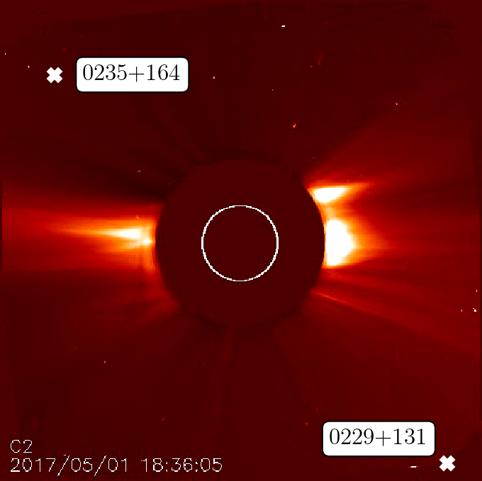
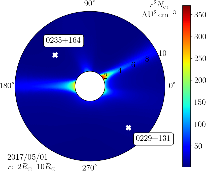
Figure 2: Observational geometry of the AUA020 session (as visible from Earth). LASCO C2 coronagraph image (left) and the solar corona electon density from the AWSoM model (right).

The AUA020 experiment was held on May 1, 2017 as part of the AUSTRAL program with the purpose of testing general relativity (Titov et al., 2018). Two radio sources that were close to the Sun were observed: 0235+164 (1.2°–1.5°) with 452 observations and 0229+131 (2.2°–2.7°) with 577 observations. The AOV022 session (May 1, 2018) featured the same two radio sources: 0235+164 (1.3°–1.6°) with 1013 observations and 0229+131 (2.0°–2.3°) with 2416 observations. Positions of the sources, coronagraph images of the solar corona , and AWSoM electron density maps for both sessions are shown in Figures 2 and 3.

The correlated VLBI data is available in the International VLBI Service for Geodesy and Astrometry (IVS) data archive .

5 VLBI data analysis

5.1 General thoughts

The quantity measured by VLBI is the group time delay between the signals arriving at two telescopes. As the signals always pass through some dispersive media with frequency-dependent refractive indexes, the total measured time delay has a dispersive term $\tau_{\mathrm{disp},f}$, which depends on the signal frequency $f$. Thus, VLBI measurements are performed at two frequencies: S band ($\approx 2.3$ GHz) and X band ($\approx 8.4$ GHz) (Sovers, 1991). If the delays measured at S and X band frequencies $f_{\mathrm{s}}$ and $f_{\mathrm{x}}$ are $\tau_{\mathrm{s}}$ and $\tau_{\mathrm{x}}$, then the expression for the dispersive contribution to $\tau_{\mathrm{x}}$ can be easily derived from eq. 11:

$$\tau_{\mathrm{disp,x}}=\frac{f_{\mathrm{s}}^{2}}{f_{\mathrm{s}}^{2}-f_{\mathrm{x}}^{2}}(\tau_{\mathrm{x}}-\tau_{\mathrm{s}}).$$ (15)

Contribution of higher-order terms in the above expression would not be greater than 0.5 mm (Hawarey et al., 2005), and, therefore, the first-order approximation is said to be accurate enough.

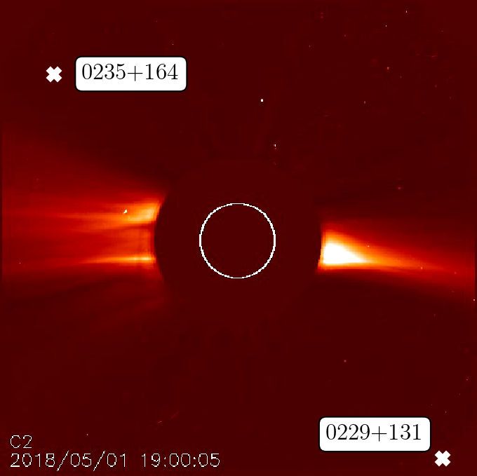
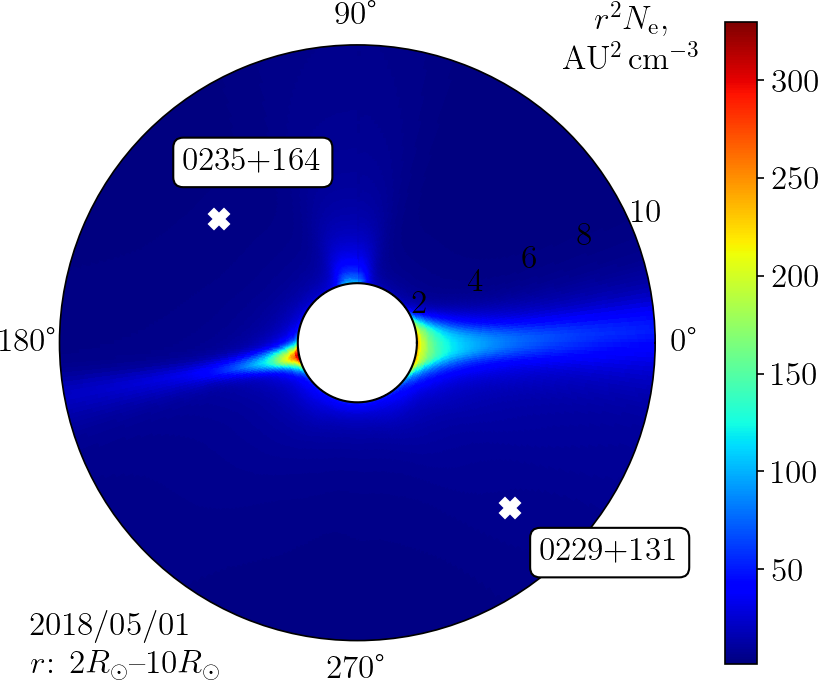
Figure 3: Observational geometry of the AOV022 session (as visible from Earth). LASCO C2 coronagraph image (left) and the solar corona electon density from the AWSoM model (right).

The dispersive term of the time delay consists of delays in intergalactic and interplanetary media, the Earth’s ionosphere, the solar corona, and receiver hardware. Delays in intergalactic and interplanetary media can be considered negligible (see Sovers, 1991, sec. 5), and therefore

$$\tau_{\mathrm{disp,x}}=\tau_{\mathrm{cor}}+\tau_{\mathrm{ion}}+\tau_{\mathrm{inst}},$$ (16)

where the three terms are the delays in the corona, the ionosphere, and receiver hardware, respectively.

Taking $N_{\mathrm{e}}(r)=0.5\cdot 10^{12}/r^{2}$ m^-3 and VLBI baseline equal to 12 000 km and perpendicular to Earth—source direction, we estimate that the coronal time delay should not be greater than 3 mm for $p=60R_{\odot}$, which corresponds to elongation of about 15°. Therefore, elongation of 15° can be chosen as a threshold above which the coronal time delay is undetectable by VLBI and is said to be equal to zero.

5.2 Ionospheric delay

The ionospheric delay $\tau_{\mathrm{ion}}$ can be obtained either by a least-squares procedure together with $\tau_{\mathrm{cor}}$ and $\tau_{\mathrm{inst}}$ (see Soja et al., 2014) or independently by using global ionosphere maps (GIMs), as done in (Soja et al., 2015), which are constructed from GPS satellite data. In this work, the second approach was followed. GIMs are routinely produced by the Center for Orbit Determination in Europe (CODE) Analysis Center (Schaer et al., 1996; Dach et al., 2018) and available via anonymous FTP server of the Astronomical Institute of University of Bern . Ionospheric model is represented by a single infinitely thin layer corresponding to the ionosphere layer F2 which has the largest charged particles density. Daily GIM files contain vertical total electron content ($E_{v}$) in TEC units (TECU); one TECU corresponds to $10^{16}$ m^-2 free electrons.

In the dual frequency VLBI observations the center frequency of X band is large compared with the local plasma frequency, therefore the contribution of ionosphere to the group delay (Ros et al., 2000) can be determined as

$$\tau_{\mathrm{ion}}=\frac{40.3\ \mathrm{m}^{3}\,\mathrm{s}^{-2}}{c\,f^{2}}\cdot E,$$ (17)

where $E$ is the total electron content along the line of sight from the radio telescope towards the target source. $E$ can be calculated from the GIM files taking into account the height of the model layer $H=450$ km above the mean Earth’s surface radius $R_{0}=6371$ km and applying the cosine mapping function

$$E=\frac{E_{v}}{\cos\arcsin\left(\frac{R}{R_{0}+H}\cos h\right)},$$ (18)

where $R$ is radius with respect to the radio telescope position and $h$ is the elevation angle of antenna pointing to the target source.

5.3 Data selection

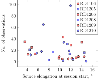
Figure 4: Elongation distribution in R&D sessions (observations at elongations above $15\degree$ are excluded).

Out of 12 R&D sessions we picked the most sensitive to the solar corona by using a criterion requiring a session to have more than 10 observations with $\tilde{\tau}_{\mathrm{cor}}>1$ cm, where $\tilde{\tau}_{\mathrm{cor}}$ is calculated using power-law model (1) with $N_{0}=10^{12}$ m^-3, $\alpha=2$. Thus, six out of 12 sessions were taken, namely, RD1106, RD1205, RD1206, RD1208, RD1209, and RD1210. The reason for such filtering is that knowing the minimum elongation for a session or even the numbers of observations for all elongations is not enough to assert sensitivity of the data to $N_{0}$. As the coronal delay depends not only on the source’s elongation, but also on the positions of the telescopes, some sort of filtering with respect to the model delay values has to be performed. Elongation distributions for the 6 picked R&D sessions are shown in Figure 4.

5.4 Algorithm

We start by taking the correlated data and subtracting the ionospoheric delays from the total delays using the procedure described in sec. 5.2. Coordinates of stations and sources are fixed to the values provided in NGS data since possible inaccuracies in the coordinates do not affect the differential delay at any significant level. To avoid correlations between the determined solar corona parameter and instrumental biases, we divide observations in each session into two groups: the first group with elongation greater than $15\degree$ and the second group with elongation less than $15\degree$. The two groups are then used in two separate solutions. In the first solution, instrumental per-station biases are determined, which define $\tau_{\mathrm{inst}}$, and in the second solution, the electron density multiplier $N_{0}$ is determined. Both adjustments are performed with weighted linear least squares procedure, which, in the case of the solution for instrumental biases, also includes iterative outlier removal by the $3\sigma$ rule. In the solution for $N_{0}$ no outlier removal is performed. Coronal delays are calculated by evaluating eq. 13 either using the analytical expression (14) (for the power-law model), or numerically (for numerical electron density maps).

We performed least-squares estimations for both the power law and the AWSoM model to see whether VLBI is able to assert the AWSoM model’s superiority over the power law. It is already known from the studies carried out by Soja et al. (2014, 2015, 2018) that VLBI observations are sensitive enough to allow for estimation of the parameters of the power-law electron density model. However, under the assumption of the power law being inaccurate and the true electron density being described by MHD models, there is still unclarity regarding the degree to which VLBI observations can be utilized in measuring real non-symmetric electron density in the corona and comparing different models. In the following section we will show that non-stationary and non-symmetric artifacts seen in MHD solutions can indeed make a noticeable impact on VLBI observations’ residuals.

6 Results

Table 2: Results

Session	Outliers	$\boldsymbol{\alpha}$	Soja et al.†	Power law††		AWSoM
			$\boldsymbol{N_{0}}$ ($\mathbf{10^{12}}$ m${}^{-3})$	$\boldsymbol{N_{0}}$ ($\mathbf{10^{12}}$ m${}^{-3})$	RMS (m)	$A$	RMS (m)
RD1106	114	2	$0.0\pm 0.4$	$0.10\pm 0.47$	0.0485	$-1.43\pm 1.28$	0.0476
RD1205	214	2	$0.5\pm 0.3$	$1.08\pm 0.21$	0.0211	$0.21\pm 0.12$	0.0223
RD1206	98	2	$0.3\pm 0.1$	$0.34\pm 0.15$	0.0288	…	…
RD1208	56	2	$1.5\pm 0.4$	$0.86\pm 0.20$	0.0315	…	…
RD1209	234	2	$0.1\pm 0.3$	$0.48\pm 0.25$	0.0497	…	…
RD1210	51	2	$2.5\pm 0.6$	$0.00\pm 0.68$	0.0482	$0.93\pm 0.80$	0.0478
AUA020	155	2.2	$0.61\pm 0.05$	$0.57\pm 0.01$	0.0655	$0.96\pm 0.02$	0.0612
AOV022	1203	2	$0.44\pm 0.005$	$0.43\pm 0.02$	0.15607	$0.84\pm 0.04$	0.1530
		2.3	…	$0.60\pm 0.03$	0.15604
${}^{\phantom{\dagger}\dagger}$ Values were taken from (Soja et al., 2014) for R&D sessions, from (Soja et al., 2018) for AUA020, and from (Soja et al., 2019) for AOV022. †† For the R&D sessions, the default value $\alpha=2$ was used. As discussed in sec. 6, residuals for these sessions do not have clear dependencies on the value of $\alpha$, and therefore it is not possible to justify a different choice of $\alpha$. For sessions AUA020 and AOV022, data shown in Figure 5 states that residuals do reach minimums at 2.2 and 2.3, respecively, so those powers were used. Power 2 for AOV022 is given only for the purpose of comparison with (Soja et al., 2019), which gives values of $N_{0}$ only for powers 2 and 2.74.

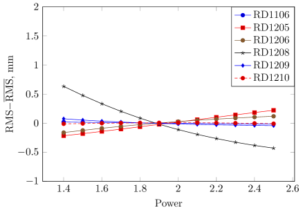
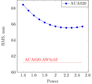
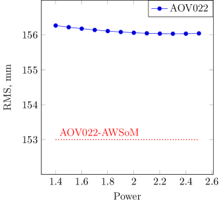
Figure 5: Dependencies of root-mean-squared (RMS) errors on the power $\alpha$ of the power-law electron density model. For each value of $\alpha$ the value of $N_{0}$ is optimal, i.e. acquired via least squares. In the left picture, each RMS curve’s average value was subtracted from the curve to clearly show dynamics of the residuals. The red dotted lines in the bottom pictures correspond to RMS errors of 0.0622 m and 0.154 m resulting from processing sessions AUA020 and AOV022 with electron density maps produced by the AWSoM model.

Solutions with the symmetric power-law model (1) were acquired for all sessions. During sessions RD1206, RD1208, and RD1209, strong coronal mass ejections (CMEs) happened, which made it impossible to apply the AWSoM data to these sessions. Because of that, solutions with the AWSoM model were obtained for all sessions except RD1206, RD1208, and RD1209. In the case of the AWSoM model, the estimated parameter was the unitless multiplier $A$ of the electron density map. The model was run with default parameters, which, as the authors have noted, need further calibration and are not guaranteed to be the best. Thus, the multiplier $A$ was artificially introduced to compensate, to some extent, for the uncertainties of the model input parameters. Values of $N_{0}$ and $A$ and their uncertainties ($1\sigma$) for each session are given in Table 2.

The values of $N_{0}$ in Table 2 generally agree within the uncertainty with the ones provided by Soja et al. (2014, 2015, 2018), and agreement is almost perfect for AUA020 and, in case of $\alpha=2$, AOV022. The only session with considerable difference in solutions is RD1210, where Soja’s result is $2.5\pm 0.6$ and ours is $0.00\pm 0.68$. In fact, taking the uncertainty into account, even these results agree within $3\sigma$. Note that the zero value of $N_{0}$ should be treated not as an actual zero electron density but as an artifact of the least-squares solution. Also, the uncertainty is large enough to cover a broad range of physically reasonable positive values of $N_{0}$.

Although least-squares estimations have succeeded at finding solutions for $N_{0}$ and confirming the results obtained independently by Soja et al. (2014, 2018, 2019), still, there is no evidence that the R&D sessions are sensitive to the choice of the solar corona model and to the parameters of the chosen model. Not only the $N_{0}$ uncertainties for the R&D sessions are somewhat large, but, as shown in Figure 5, the post-fit residuals barely depend on the choice of the power $\alpha$, varying by less than 0.5–1 mm with $\alpha$ changing from 1.4 to 2.5 and not even reaching minimum values for any given $\alpha$. Hence, from the perspective of the R&D sessions data, all possible power laws fit the electron density equally well, including those with extreme $\alpha$ values that never occur in previously published papers and therefore seem unlikely in general. Furthermore, the residuals for the R&D sessions with the AWSoM model (given in Table 2) differ only slightly from those for the power law and fail to show any consistent relationship to them.

To put it differently, we are faced with an ultimate impossibility to reliably determine any solar corona parameters from the R&D sessions. The power $\alpha$ is indeterminable since for virtually any $\alpha$ there exists an optimal $N_{0}(\alpha)$ which fits the observations almost equally well as any other optimal $(\alpha,\,N_{0}(\alpha))$ pair. And even if we assume $\alpha$ to be fixed and accurate, the estimated values of $N_{0}$ differ greatly between different sessions and uncertainties cover wide ranges of $N_{0}$, making the solutions reliable only in a purely mathematical sense and disconnected from physical reality.

A session that appears to be sensitive to the electron density models is AUA020. The reasons for that have to be (i) a fairly large number of observations close to the Sun and (ii) outstandingly small elongation angles. The uncertainty of $N_{0}$ is by an order of magnitude smaller than the uncertainties for the R&D sessions, and, importantly, the dependency of residuals on the power $\alpha$ (Figure 5) clearly shows a minimum at $\alpha\approx 2.2$. With the AWSoM model, the residuals for AUA020 decrease by $\approx 4$ mm, which means that the model eliminates a scatter of 2 cm in root-mean-square sense and therefore might be considered to be a significant improvement over the power-law model.

The situation is quite similar with the AOV022 session, which also shows a residuals minimum at $\alpha\approx 2.2$, sufficiently small estimated parameter uncertainties, and a 3 mm decrease in residuals with the AWSoM model.

7 Conclusion and future work

We have shown that the VLBI technique is capable of providing observational data sensitive enough to the solar corona electron density to distinguish between different models and to allow for estimation of model parameters. However, VLBI sessions need to be planned carefully to include a large number of observations at small heliocentric distances, since VLBI’s sensitivity to the solar corona decreases severely at elongations even as large as 4°, as we have seen in the case of R&D sessions.

Having confirmed recent results of (Soja et al., 2014, 2015, 2018), we also note that the AUA020 and AOV022 sessions show superiority of the AWSoM model over the power law, and suggest that the power law is not an accurate representation of the solar corona electron density and that further analysis can significantly benefit from more sophisticated modern 3D solar corona models. The AWSoM model results were successfully compared to different kinds of observations in multiple works (see e.g. Sokolov et al., 2013; Oran et al., 2013; Moschou et al., 2018); VLBI observations of quasars provide an additional source of validation. A more careful analysis is needed in presence of strong coronal mass ejections (CMEs), where AWSoM data suggests extremely high electron density in certain regions. Currently, the available VLBI observations do not fit to the numerical model with strong CMEs as well as they do with a symmetric model.

The R&D sessions have proved to be unable to determine anything but the mere fact that the solar corona exists and that its electron density decreases with heliospheric distance, which is already a universally accepted truth. To fully explore the possibilities that VLBI provides for comparing different solar corona models, there has to be more observational data available, preferably of the likes of AUA020 and AOV022 in terms of the number of observations made close to the Sun and minimum elongation angles. As Titov et al. (2018) point out, that requires strong radio sources being close to the Sun, and also large radio telescopes and high data recording rate.

References

- Anderson et al. (1987) Anderson, J. D., Krisher, T. P., Borutzki, S. E., et al. 1987, The Astrophysical Journal, 323, L141, doi: 10.1086/185074
- Bale et al. (2016) Bale, S. D., Goetz, K., Harvey, P. R., et al. 2016, Space Science Reviews, 204, 49, doi: 10.1007/s11214-016-0244-5
- Berman (1977) Berman, A. L. 1977, Electron Density in the Extended Corona: Two Views, The deep space network progress report 42-41, NASA JPL
- Bird & Edenhofer (1990) Bird, M. K., & Edenhofer, P. 1990, Remote Sensing Observations of the Solar Corona, ed. R. Schwenn & E. Marsch (Springer Berlin Heidelberg), 13–97
- Bird et al. (2012) Bird, M. K., Pätzold, M., Häusler, B., et al. 2012, in 511th WE-Heraeus-Seminar, Physikzentrum Bad Honnef, Germany. http://www2.mps.mpg.de/meetings/hcor/p/p01.pdf
- Cranmer et al. (2007) Cranmer, S., A. van Ballegooijen, A., & Edgar, R. 2007, The Astrophysical Journal Supplement Series, 171, doi: 10.1086/518001
- Cranmer (2002) Cranmer, S. R. 2002, Space Science Reviews, 101, 229, doi: 10.1023/A:1020840004535
- Dach et al. (2018) Dach, R., Schaer, S., Jäggi, A., et al. 2018, CODE final product series for the IGS, Astronomical Institute, University of Bern, doi: 10.7892/boris.75876.3. https://boris.unibe.ch/119490/
- Goldston & Rutherford (1995) Goldston, R. J., & Rutherford, P. H. 1995, Introduction to Plasma Physics (Bristol, UK Philadelphia: Institute of Physics Publishing)
- Harrison et al. (2008) Harrison, R. A., Davis, C. J., Eyles, C. J., et al. 2008, Solar Physics, 247, 171, doi: 10.1007/s11207-007-9083-6
- Hawarey et al. (2005) Hawarey, M., Hobiger, T., & Schuh, H. 2005, Geophysical Research Letters, 32, doi: 10.1029/2005GL022729
- Kelso (1959) Kelso, J. 1959, Journal of Atmospheric and Terrestrial Physics, 16, 357, doi: 10.1016/0021-9169(59)90085-6
- Mayer et al. (2014) Mayer, D., Böhm, J., Combrinck, L., Botai, J., & Böhm, S. 2014, Acta Geodaetica et Geophysica, 49, 313, doi: 10.1007/s40328-014-0063-7
- Meyer-Vernet (2007) Meyer-Vernet, N. 2007, Basics of the Solar Wind, Cambridge Atmospheric and Space Science Series (Cambridge University Press), doi: 10.1017/CBO9780511535765
- Moschou et al. (2018) Moschou, S.-P., Sokolov, I., Cohen, O., et al. 2018, The Astrophysical Journal, 867, 51, doi: 10.3847/1538-4357/aae58c
- Nothnagel et al. (2017) Nothnagel, A., Artz, T., Behrend, D., & Malkin, Z. 2017, Journal of Geodesy, 91, 711, doi: 10.1007/s00190-016-0950-5
- Oran et al. (2013) Oran, R., van der Holst, B., Landi, E., et al. 2013, The Astrophysical Journal, 778, 176, doi: 10.1088/0004-637x/778/2/176
- Parker (1958) Parker, E. N. 1958, The Astrophysical Journal, 128, 664, doi: 10.1086/146579
- Perlick (2000) Perlick, V. 2000, Ray Optics, Fermat’s Principle, and Applications to General Relativity, Lecture Notes in Physics Monographs (Springer)
- Pierrard et al. (1999) Pierrard, V., Maksimovic, M., & Lemaire, J. 1999, Journal of Geophysical Research: Space Physics, 104, 17021, doi: 10.1029/1999JA900169
- Plank et al. (2017) Plank, L., Lovell, J. E. J., McCallum, J. N., et al. 2017, Journal of Geodesy, 91, 803, doi: 10.1007/s00190-016-0949-y
- Ros et al. (2000) Ros, E., Marcaide, J. M., Guirado, J. C., Sardón, E., & Shapiro, I. I. 2000, Astronomy and Astrophysics, 356, 357
- Schaer et al. (1996) Schaer, S., Beutler, G., Rothacher, M., & Springer, T. A. 1996, in Proceedings of the IGS Analysis Center Workshop 1996, ed. R. Neilan, P. Van Scoy, & J. Zumberge, 181–192
- Schuh & Behrend (2012) Schuh, H., & Behrend, D. 2012, Journal of Geodynamics, 61, 68, doi: 10.1016/j.jog.2012.07.007
- Shuygina et al. (2019) Shuygina, N., Ivanov, D., Ipatov, A., et al. 2019, Geodesy and Geodynamics, 10, 150, doi: 10.1016/j.geog.2018.09.008
- Soja et al. (2014) Soja, B., Heinkelmann, R., & Schuh, H. 2014, Nature Communications, 5, doi: 10.1038/ncomms5166
- Soja et al. (2015) Soja, B., Heinkelmann, R., & Schuh, H. 2015, in IAG 150 Years (Cham: Springer International Publishing), 611–616
- Soja et al. (2018) Soja, B., Titov, O., Girdiuk, A., et al. 2018, Solar Corona Electron Density Models from Recent VLBI Experiments AUA020 and AUA029, doi: 10.13140/rg.2.2.21438.38728
- Soja et al. (2019) Soja, B., Heinkelmann, R., H. Schuh, et al. 2019, Very Long Baseline Interferometry as a tool to probe the solar corona, Unpublished, doi: 10.13140/rg.2.2.17735.04009. http://rgdoi.net/10.13140/RG.2.2.17735.04009
- Sokolov et al. (2013) Sokolov, I. V., van der Holst, B., Oran, R., et al. 2013, The Astrophysical Journal, 764, 23, doi: 10.1088/0004-637x/764/1/23
- Sovers (1991) Sovers, O. J. 1991, Observation model and parameter partials for the JPL VLBI parameter estimation software MODEST/1991, JPL publication 83-39 rev. 4, NASA
- Taktakishvili et al. (2011) Taktakishvili, A., Pulkkinen, A., MacNeice, P., et al. 2011, Space Weather, 9, doi: 10.1029/2010SW000642
- Thompson (2006) Thompson, W. T. 2006, Astronomy & Astrophysics, 449, 791, doi: 10.1051/0004-6361:20054262
- Titov et al. (2018) Titov, O., Girdiuk, A., Lambert, S. B., et al. 2018, Astronomy & Astrophysics, 618, A8, doi: 10.1051/0004-6361/201833459
- Tóth et al. (2012) Tóth, G., van der Holst, B., Sokolov, I. V., et al. 2012, Journal of Computational Physics, 231, 870, doi: 10.1016/j.jcp.2011.02.006
- van der Holst et al. (2014) van der Holst, B., Sokolov, I. V., Meng, X., et al. 2014, The Astrophysical Journal, 782, 81, doi: 10.1088/0004-637x/782/2/81