Abstract

A supersymmetric hybrid inflation framework is employed to realize a class of non-minimal inflation models with $U(1)_{R}\times Z_{n}$ global symmetry. This framework naturally incorporates models based on grand unified theories by avoiding the most commonly faced monopole problem. The predictions of inflationary observables, the scalar spectral index $n_{s}=0.960-0.966$ and the tensor to scalar ratio $r=0.0031-0.0045$, are in perfect agreement with the Planck 2018 data. For sub-Planckian values of the field the $Z_{n}$ symmetry is only allowed for $n\leq 4$.

1 Introduction

One of the most favored inflationary model according to Planck 2018 results [1] is the Starobinsky model [2]. The scalar field version of this model is equivalent to an inflationary model which exploits a strong non-minimal coupling of the scalar field with gravity. See for example [3, 4] for a few of the non-supersymmetric models of non-minimal Higgs inflation. In order to realize non-minimal inflation in supersymmetric framework a special form of Kähler potential is employed. For the feasibility of realizing inflation with standard model like Higgs boson in the minimal supersymmetric standard model see [5, 6, 7]. Further this idea has also been applied to Higgs fields in grand unified theories (GUTs) [8, 9].

The supersymmetric hybrid inflation model provides an elegant framework to incorporate GUTs [10][11][12]. However, the standard version of supersymmetric hybrid inflation is plagued with the monopole problem which is a generic prediction of GUTs based on a simple gauge group. In this paper we effectively consider a model of non-minimal GUT Higgs inflation with a special form of Kähler potential that is usually employed in no-scale supergravity models [13]. In this model monopoles are produced during inflation and are inflated away. The viability of non-minimal inflation is explored in a broader context with an additional $Z_{n}$ symmetry. The predictions of various inflationary parameters are obtained in a generic GUT framework and are consistent with the Planck 2018 results.

2 Superpotential with $U(1)_{R}\times Z_{n}$ Symmetry

In a typical supersymmetric hybrid inflation framework based on a given GUT gauge group, $G$, we usually consider a gauge singlet superfield, $S$, along with a gauge non-singlet conjugate pair of Higgs superfields $H$ and $\overline{H}$. Some of the examples of the GUT gauge groups are $SO(10)$, $SU(5)\times U(1)$ and $SU(4)_{c}\times SU(2)_{L}\times SU(2)_{R}$ with Higgs superfields residing in the $16,10$ and $(4,1,2)$ dimensional representations of the respective gauge groups [14]. With this minimal content of superfields and the $U(1)_{R}\times Z_{n}$ global symmetry we obtain the following simple form of the superpotential [15, 16],

$$W=\kappa S\left(-\mu^{2}+\frac{\left(H\overline{H}\right)^{m}}{\Lambda^{2m-2}}\right).$$ (1)

Here, $\kappa$ is a dimensionless coupling, $\mu$ is some superheavy mass and $\Lambda$ is the cut-off scale. Under $Z_{n}$ symmetry the superfield, $S$, carries zero charge whereas Higgs superfields carry unit charges. This makes the integer $m=n$ for odd values of $n$ and $m=n/2$ for even values of $n$ [16]. For example, values of $m=1,2,3$ correspond to $n=2,4,3$ respectively. However, for the special case of $m=1$ we do not need to impose any $Z_{2}$ symmetry as GUT gauge symmetry alone is sufficient to restrict the form of the superpotential. Further, the superfield $S$ and the superpotential $W$ carry one unit of $R$ charge whereas $H\overline{H}$ is neutral under $U(1)_{R}$ symmetry. This $R$ charge assignment ensures a linear relationship of $W$ in terms of $S$ which is necessary to realize a consistent model of inflation [10].

The global supersymmetric minimum occurs at

$$\left<S\right>=0,\,\,\,\left<\left(H\overline{H}\right)^{m}\right>=M^{2m}\equiv\mu^{2}\Lambda^{2m-2},$$ (2)

where the Higgs vacuum expectation value (VEV) is described by $M$. This gauge symmetry breaking scale is taken to be the GUT scale, $M_{GUT}\equiv 2\times 10^{16}$ GeV, in our numerical calculations. Further we set $\Lambda=m_{P}$ where $m_{P}=2\times 10^{18}$ GeV is the reduced Planck mass.

The form of the superpotential considered above has been used before mostly in the context of new inflation in a supersymmetric framework. Once the field $S$ is stabilized we obtain an effective Higgs potential which, for values of fields below $M$, can be used for new inflation. For example, see [15] where it is used to realize pre-inflation in order to justify the initial conditions of new inflation. In ref. [16], it was used to realize a model of new inflation itself. In ref. [17], flavon inflation is discussed using a similar form of the superpotential. For $SU(5)$ and flipped $SU(5)$ based GUT realization of new inflation see [18]. In this paper, however, we consider the other side of the Higgs potential where field values lie above $M$ and the potential is steep. A special form of the Kähler potential, which is usually employed in the no-scale gravity models, helps to reduce the slope of the potential and makes it suitable for the slow-roll conditions to apply. This setup gives rise to non-minimal Higgs inflation which is discussed below in detail with additional $Z_{n}$ symmetry.

3 Non-minimal Higgs Inflation with $Z_{n}$ Symmetry

To achieve non-minimal inflation we consider the following special form of the Kähler potential

$$\begin{split}K&=-3m_{P}^{2}\log\Bigg{(}1-\frac{(|S|^{2}+|H|^{2}+|\overline{H}|^{2})}{3m_{P}^{2}}+\frac{\chi}{2m_{P}^{2}}\Big{(}\frac{(H\overline{H})^{m}}{\Lambda^{2m-2}}+h.c\Big{)}+\gamma\frac{|S|^{4}}{3m_{P}^{4}}\Bigg{)},\end{split}$$ (3)

where $\chi$ and $\gamma$ are dimensionless parameters. This is a variant of the Kähler potential usually employed in the no-scale supergravity models where moduli fields are assumed to be stabilized [13]. The addition of last term is necessary for the stabilization of $S$ field [7]. The scalar potential and the metric in Jordan and Einstein frames are related via the conformal rescaling factor $\Omega^{2}=e^{-K/3m_{P}^{2}}$ as,

$$V_{J}=\Omega^{4}V_{E},\quad\quad g_{J}^{\mu\nu}=\Omega^{2}g_{E}^{\mu\nu}.$$ (4)

This defines the Einstein-frame scalar potential $V_{E}$ in terms of $W$ and $K$ as

$$V_{E}=e^{K/m_{P}^{2}}\left(K_{ij}^{-1}D_{z_{i}}WD_{z_{j}^{*}}W^{*}-3m_{P}^{-2}|W|^{2}\right)+V_{D}^{E},$$ (5)

where

$$D_{z_{i}}W=\frac{\partial W}{\partial z_{i}}+\frac{1}{m_{P}^{2}}\frac{\partial K}{\partial z_{i}}W,\quad K_{ij}=\frac{\partial^{2}K}{\partial z_{i}\partial z_{j}^{*}},\quad D_{z_{j}^{*}}W^{*}=(D_{z_{i}}W)^{*},$$ (6)

with $z_{i}\in\{S,H,\overline{H}\}$. Here, same notation has been used for the superfields and their scalar components. The Einstein-frame D-term potential is given by

$$V_{D}^{E}\propto g^{2}\,(|H|^{2}-|\overline{H}|^{2}).$$ (7)

Writing complex Higgs fields in terms of real scalar fields,

$$H=\frac{\phi}{\sqrt{2}}\ e^{i\alpha}\cos\beta,\qquad\overline{H}=\frac{\phi}{\sqrt{2}}\ e^{i\overline{\alpha}}\sin\beta,$$ (8)

the stabilized D-flat direction is obtained for $\beta=\pi/4$, $\alpha=\overline{\alpha}=0$ and this implies that

$$H=\overline{H}=\frac{\phi}{2},$$ (9)

where $\phi$ is the canonically normalized real scalar field in the Jordan frame. Finally the scalar potential in the Einstein frame takes the following form

$$V_{E}=\frac{\kappa^{2}\mu^{4}\left(1-\left(\frac{\phi}{2M}\right)^{2m}\right)^{2}}{\left(1-\frac{2}{3}\left(\frac{\phi}{2m_{P}}\right)^{2}+\chi\left(\frac{\phi}{2m_{P}}\right)^{2m}\right)^{2}}.$$ (10)

After conformal rescaling the canonically normalized inflaton field $\hat{\phi}(\phi)$ in the Einstein frame becomes a function of field $\phi$ as

$$J(\phi)\equiv\left(\frac{d\hat{\phi}}{d\phi}\right)=\sqrt{\frac{1}{\Omega^{2}(\phi)}+\frac{3}{2}m_{P}^{2}\left(\frac{d\ln\Omega^{2}(\phi)}{d\phi}\right)^{2}}.$$ (11)

The slow-roll parameters can now be expressed in terms of $\phi$ as

$$\epsilon(\phi)=\frac{1}{2}m_{P}^{2}\left(\frac{V_{E}^{\prime}}{JV_{E}}\right)^{2},\quad\eta(\phi)=m_{P}^{2}\Bigg{(}\frac{V_{E}^{\prime\prime}}{J^{2}V_{E}}-\frac{J^{\prime}V_{E}^{\prime}}{J^{3}V_{E}}\Bigg{)},$$ (12)

where a prime denotes a derivative with respect to $\phi$. The scalar spectral index $n_{s}$ and the tensor to scalar ratio $r$ to the first order in slow-roll approximation are given by

$$n_{s}\simeq 1-6\epsilon(\phi_{0})+2\eta(\phi_{0}),\qquad r\simeq 16\epsilon(\phi_{0}),$$ (13)

where the field value, $\phi_{0}$, corresponds to the number of e-folds,

$$N_{0}=\frac{1}{\sqrt{2}m_{P}}\int_{\phi_{e}}^{\phi_{0}}\dfrac{J(\phi)}{\sqrt{\epsilon(\phi)}}d\phi,$$ (14)

before the end of inflation at $\phi=\phi_{e}$ defined by the condition $\epsilon(\phi_{e})=1$. Also, $\phi_{0}$ corresponds to the pivot scale where the amplitude of the scalar power spectrum is normalized by Planck [1] to be,

$$A_{s}(k_{0})=\left.\frac{1}{24\,\pi^{2}\epsilon(\phi)}\frac{V_{E}(\phi)}{m_{P}^{4}}\right|_{\phi(k_{0})=\phi_{0}}=2.137\times 10^{-9},$$ (15)

at $k_{0}=0.05\,\text{Mpc}^{-1}$. For non-minimal inflation with sub-Planckian values of the field we need to consider the large $\chi$ limit such that $\chi\left(\frac{\phi}{m_{P}}\right)^{2m}\gg 1$. Therefore, in the non-minimal limit with $\phi_{0}\gg M$, above relation can be used to eliminate $\kappa$ in terms of $\phi_{0}$ as

$$\kappa\simeq\chi\sqrt{24\pi^{2}A_{s}(k_{0})\epsilon(\phi_{0})}\simeq\sqrt{32\pi^{2}A_{s}(k_{0})}\left(\frac{2m_{P}}{\phi_{0}}\right)^{2m}.$$ (16)

Now we look for a relation of $\phi_{0}$ in terms of $N_{0}$. Using Eq. (14) and $\epsilon(\phi_{e})=1$, the field values $\phi_{0}$ and $\phi_{e}$ can be written in terms of $N_{0}$ as

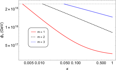
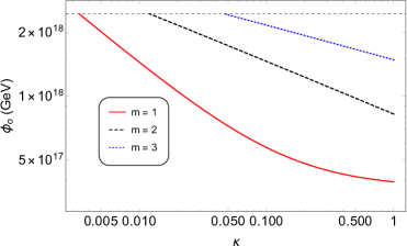
Figure 1: The variation of field value $\phi_{0}$ versus $\kappa$ for $m=1,2,3$ and $N_{0}=50$(left panel), $60$(right panel). We set the gauge symmetry breaking scale $M=2\times 10^{16}$ GeV.

$$\frac{\phi_{0}}{2m_{P}}\simeq\left(\frac{4N_{0}}{3\chi}\right)^{1/2m},\quad\frac{\phi_{e}}{2m_{P}}\simeq\left(\frac{4}{3\chi^{2}}\right)^{1/4m}.$$ (17)

Therefore, field values are expected to change with $m$ or $Z_{n}$ symmetry. This is confirmed by the exact numerical results shown in the Fig. (1) for the variation of $\phi_{0}$ with respect to $\kappa$. With sub-Planckian field values $\phi_{0}\lesssim m_{P}$ we obtain $\chi\gtrsim\frac{2^{2m+2}}{3}N_{0}\gg 1$ which provides a cross-check for using the large $\chi$ limit at first place. Using again above value of $\phi_{0}$ in Eq. (16) we obtain a constant value for the ratio $\kappa/\chi$ written in terms of $N_{0}$ as

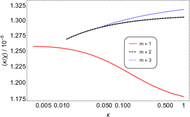
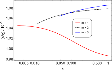
Figure 2: The ratio $\kappa/\chi$ versus $\kappa$ for $m=1,2,3$ and $N_{0}=50$ (left panel), $60$(right panel). We set the gauge symmetry breaking scale $M=2\times 10^{16}$ GeV.

$$\kappa/\chi\simeq\frac{3\sqrt{2\pi^{2}A_{s}(k_{0})}}{N_{0}}\simeq\left\{\begin{array}[]{ll}1.23\times 10^{-5}&\mbox{for $N_{0}=50,$}\\ 1.03\times 10^{-5}&\mbox{for $N_{0}=60$}.\end{array}\right.$$ (18)

This ratio turns out to be of order $10^{-5}$ showing a weak dependence on $m$ or $Z_{n}$ symmetry in the non-minimal limit and this can also be seen in our numerical results displayed in the Fig. (2). We can express field value $\phi_{0}$ in terms of $\kappa$ using Eq. (18) in Eq. (17) as

$$\frac{\phi_{0}}{m_{P}}\simeq 2\left(\frac{4N_{0}/\kappa}{3\times 10^{5}}\right)^{1/2m}.$$ (19)

For a given value of $\kappa$, this expression explains the observed increasing trend of field values with respect to $m$ as shown in Fig. 1. This trend leads to fine tuning in the solutions with large values of $m$ as soon as $\phi_{0}$ becomes tran-Planckian. Therefore, we allow $m\leq 3$ or $n\leq 4$ for $\phi_{0}\lesssim m_{P}$ with perturbative values of $\kappa\lesssim 0.1$. For $SU(5)$ GUT with Higgs field in the adjoint representation we expect to obtain two more solutions for $m=3/2$ and $m=5/2$ effectively.

Finally, the expression of $\phi_{0}$ is used to obtain the scalar spectral index $n_{s}$ and the tensor to scalar ratio $r$ in terms of $N_{0}$,

$$n_{s}\simeq 1-\frac{2}{N_{0}}\simeq\left\{\begin{array}[]{ll}0.960&\mbox{for $N_{0}=50,$}\\ 0.967&\mbox{for $N_{0}=60$},\end{array}\right.\quad r\simeq\frac{12}{N_{0}^{2}}\simeq\left\{\begin{array}[]{ll}0.0048&\mbox{for $N_{0}=50,$}\\ 0.0033&\mbox{for $N_{0}=60$},\end{array}\right.$$ (20)

where, $\epsilon(\phi_{0})=\frac{3}{4N_{0}^{2}}$ and $\eta(\phi_{0})=-\frac{1}{N_{0}}$. This result holds in the leading order approximation and also explains the weak dependence of $n_{s}$ and $r$ on $m$ or $Z_{n}$ symmetry as confirmed by our numerical estimates displayed in Table-I. We show the predictions of various inflationary parameters in Table-I, using first order slow-roll approximation, for $\kappa=0.1$, $M=2\times 10^{16}$ GeV and $N_{0}=(50,60)$. We obtain $n_{s}\simeq 0.96\,(0.966)$ and $r\simeq 0.0045\,(0.0031)$ for $N_{0}=50\,(60)$ respectively, independent of $m$ and $\kappa$ values. The non-minimal coupling parameter is large $\chi\sim 10^{5}$ and this is a common feature of these models. An order of magnitude estimate of error expectancy in inflationary parameters can be calculated from the second order slow-roll contribution. This can be described as a fractional change in the corresponding quantity, e.g., $\Delta n_{s}/n_{s}\simeq 0.01\%$, $\Delta r/r\simeq 1.5\%$, $\Delta\phi/\phi\simeq 0.4\%$, $\Delta\chi/\chi\simeq 1\%$.

For $N_{0}$ = 50
	$r$	$n_{s}$	$\phi_{0}$	$\phi_{e}$	$\chi$
$m=1$	0.0045	0.960	$5.5\times 10^{17}$	$7.4\times 10^{16}$	$8194$
$m=2$	0.0051	0.957	$1.4\times 10^{18}$	$4.0\times 10^{17}$	$7718$
$m=3$	0.0051	0.957	$2.1\times 10^{18}$	$8.6\times 10^{17}$	$7693$
For $N_{0}$ = 60
$m=1$	0.0031	0.966	$5.7\times 10^{17}$	$7.2\times 10^{16}$	$9848$
$m=2$	0.0035	0.965	$1.4\times 10^{18}$	$3.8\times 10^{17}$	$9337$
$m=3$	0.0035	0.964	$2.2\times 10^{18}$	$8.3\times 10^{17}$	$9331$

Table 1: The predicted values of inflationary parameters with gauge symmetry breaking scale $M=2\times 10^{16}$GeV and $\kappa=0.1$.

4 Conclusion

We have studied a class of models based on the realization of non-minimal inflation in $R$-symmetric supersymmetric hybrid inflation framework with an additional $Z_{n}$ symmetry. The requirement of sub-Planckian field values is satisfied in the large $\chi$ limit. This also restricts the possible values of $n\leq 4$ with $\kappa\lesssim 0.1$. We have calculated the predictions of $n_{s}$ and $r$ numerically and also provided the analytic justification of these results. Finally, we conclude that the results of non-minimal inflation hold in a rather broad class of supersymmetric GUT models.

References

- [1] Y. Akrami et al. [Planck Collaboration], arXiv:1807.06211 [astro-ph.CO].
- [2] A. A. Starobinsky, Phys. Lett. B 91, 99 (1980) [Phys. Lett. 91B, 99 (1980)] [Adv. Ser. Astrophys. Cosmol. 3, 130 (1987)].
- [3] F. L. Bezrukov, A. Magnin and M. Shaposhnikov, Phys. Lett. B 675, 88 (2009) doi:10.1016/j.physletb.2009.03.035 [arXiv:0812.4950 [hep-ph]]; A. De Simone, M. P. Hertzberg and F. Wilczek, Phys. Lett. B 678, 1 (2009) doi:10.1016/j.physletb.2009.05.054 [arXiv:0812.4946 [hep-ph]]; A. O. Barvinsky, A. Y. Kamenshchik, C. Kiefer, A. A. Starobinsky and C. Steinwachs, JCAP 0912, 003 (2009) doi:10.1088/1475-7516/2009/12/003 [arXiv:0904.1698 [hep-ph]]; N. Okada, M. U. Rehman and Q. Shafi, arXiv:0911.5073 [hep-ph].
- [4] N. Okada, M. U. Rehman and Q. Shafi, Phys. Rev. D 82, 043502 (2010) doi:10.1103/PhysRevD.82.043502 [arXiv:1005.5161 [hep-ph]]; A. Linde, M. Noorbala and A. Westphal, JCAP 1103, 013 (2011) doi:10.1088/1475-7516/2011/03/013 [arXiv:1101.2652 [hep-th]]; N. Okada, M. U. Rehman and Q. Shafi, Phys. Lett. B 701, 520 (2011) doi:10.1016/j.physletb.2011.06.044 [arXiv:1102.4747 [hep-ph]]; C. Pallis and Q. Shafi, JCAP 1503, no. 03, 023 (2015) doi:10.1088/1475-7516/2015/03/023 [arXiv:1412.3757 [hep-ph]]; N. Bostan, Ö. Güleryüz and V. N. Şenoğuz, JCAP 1805, no. 05, 046 (2018) doi:10.1088/1475-7516/2018/05/046 [arXiv:1802.04160 [astro-ph.CO]]; N. Bostan and V. N. Şenoğuz, arXiv:1907.06215 [astro-ph.CO].
- [5] M. B. Einhorn and D. R. T. Jones, JHEP 1003, 026 (2010) doi:10.1007/JHEP03(2010)026 [arXiv:0912.2718 [hep-ph]].
- [6] S. Ferrara, R. Kallosh, A. Linde, A. Marrani and A. Van Proeyen, Phys. Rev. D 82, 045003 (2010) doi:10.1103/PhysRevD.82.045003 [arXiv:1004.0712 [hep-th]].
- [7] H. M. Lee, JCAP 1008, 003 (2010) doi:10.1088/1475-7516/2010/08/003 [arXiv:1005.2735 [hep-ph]].
- [8] C. Pallis and N. Toumbas, JCAP 1112, 002 (2011) doi:10.1088/1475-7516/2011/12/002 [arXiv:1108.1771 [hep-ph]].
- [9] W. Ahmed and A. Karozas, Phys. Rev. D 98 (2018) no.2, 023538 doi:10.1103/PhysRevD.98.023538 [arXiv:1804.04822 [hep-ph]].
- [10] G. R. Dvali, Q. Shafi and R. K. Schaefer, Phys. Rev. Lett. 73, 1886 (1994) [hep-ph/9406319].
- [11] E. J. Copeland, A. R. Liddle, D. H. Lyth, E. D. Stewart and D. Wands, Phys. Rev. D 49, 6410 (1994) [astro-ph/9401011].
- [12] A. D. Linde and A. Riotto, Phys. Rev. D 56, R1841 (1997) [hep-ph/9703209]; V. N. Senoguz and Q. Shafi, Phys. Rev. D 71, 043514 (2005) doi:10.1103/PhysRevD.71.043514 [hep-ph/0412102]; M. U. Rehman, Q. Shafi and J. R. Wickman, Phys. Lett. B 683, 191 (2010) doi:10.1016/j.physletb.2009.12.010 [arXiv:0908.3896 [hep-ph]].
- [13] J. Ellis, D. V. Nanopoulos and K. A. Olive, Phys. Rev. Lett. 111, 111301 (2013) Erratum: [Phys. Rev. Lett. 111, no. 12, 129902 (2013)] doi:10.1103/PhysRevLett.111.129902, 10.1103/PhysRevLett.111.111301 [arXiv:1305.1247 [hep-th]].
- [14] V. N. Senoguz and Q. Shafi, Phys. Lett. B 567, 79 (2003) doi:10.1016/j.physletb.2003.06.030 [hep-ph/0305089].
- [15] M. Yamaguchi and J. Yokoyama, Phys. Rev. D 70, 023513 (2004) doi:10.1103/PhysRevD.70.023513 [hep-ph/0402282].
- [16] V. N. Senoguz and Q. Shafi, Phys. Lett. B 596, 8 (2004) doi:10.1016/j.physletb.2004.05.077 [hep-ph/0403294].
- [17] S. Antusch, S. F. King, M. Malinsky, L. Velasco-Sevilla and I. Zavala, Phys. Lett. B 666, 176 (2008) doi:10.1016/j.physletb.2008.07.051 [arXiv:0805.0325 [hep-ph]].
- [18] M. U. Rehman, M. M. A. Abid and A. Ejaz, arXiv:1804.07619 [hep-ph].