A compositional semantics for Repairable Fault Trees with general distributions

Abstract

Fault Tree Analysis (FTA) is a prominent technique in industrial and scientific risk assessment. Repairable Fault Trees (RFT) enhance the classical Fault Tree (FT) model by introducing the possibility to describe complex dependent repairs of system components. Usual frameworks for analyzing FTs such as BDD, SBDD, and Markov chains fail to assess the desired properties over RFT complex models, either because these become too large, or due to cyclic behaviour introduced by dependent repairs. Simulation is another way to carry out this kind of analysis. In this paper we review the RFT model with Repair Boxes as introduced by Daniele Codetta-Raiteri. We present compositional semantics for this model in terms of Input/Output Stochastic Automata, which allows for the modelling of events occurring according to general continuous distribution. Moreover, we prove that the semantics generates (weakly) deterministic models, hence suitable for discrete event simulation, and prominently for Rare Event Simulation using the FIG tool.

1 Introduction

Fault Tree Analysis is a prominent technique for dependability assessment of complex industrial systems. Standard or Static Fault Trees (SFTs [21]) are DAGs whose leafs are called Basic Events (BE), and usually represent the failure of a physical system component. Each leaf is equipped with a failure rate or discrete probability, indicating the frequency at which the component breaks. The other FT nodes are called gates, and they model how basic components failures combine to induce more complex system failures, until the failure of interest (the top event of the tree) occurs. SFTs thus encode a logical formula. One of the most efficient analysis techniques uses Binary Decision Diagrams (BDD) to represent the formula, and then perform dependability studies using specialised algorithms. This assumes the absence of stochastic dependency among BEs.

Many extensions to SFTs allow for further modelling capabilities. One of the most studied are Dynamic Fault Trees (DFTs [16, 22]). DFTs add gates to describe time- and order-dependence among the tree nodes, in contrast to the plain combinatorial behavior of SFT gates. New analysis methods were introduced in order to capture temporal requirements, such as cut sequences, translation to Markov models [16, 16, 6], Sequence BDDs [19, 28, 35], algebraic approaches [25, 1], simulation, and combination and optimisations thereof [3, 20].

Repairable Fault Trees (RFT [4, 27, 2, 6]) increase FTs expressiveness by introducing the possibility to model complex inter-dependent repair mechanisms for basic components, i.e. system components that produce the basic events. In former models such as DFT, certain notions of repair had been addressed by allowing components to be repaired independently. Nevertheless, this is not usual in real world systems, where repair scheduling, resources management, and maintenance play an important role. To address this, we will focus on the Repair Box model (RBOX [18, 27]). A RBOX models a repair unit in charge of repairing certain BEs following certain policy. Different repair policies such as first come first serve, priority service, random or nondeterministic choice, allow to analyze the impact of taking these decisions in the real system. The introduction of these boxes greatly changes the dynamic of the tree. Quantitative analyses are no longer a combinatorial calculation, since the evolution of the system over time has to be considered [32]. Furthermore, traditional qualitative analysis such as cut sets lack of utility by not taking repairability into account. Traditional quantitative analysis is also discarded by the cyclic behavior introduced by this model which disallows to use combinatorial solutions proposed for non repairable FTs and require a state based solution instead [3].

In this work we present a formal definition of Repairable Fault Trees (RFT), along with its semantics given in terms of Input/Output Stochastic Automata (IOSA) [15, 17]. We show that the underlying IOSA semantics of the RFT specification is weakly deterministic, that is, the non-determinism present in the IOSA model is spurious. Hence the model is equivalent to a fully stochastic model and thus amenable to discrete event simulation. IOSA allows us to model RFTs general continuous failure and repair distributions.

A variety of works address the problem of defining a rigorous syntax and semantics to FT, DFT, and RFT [14, 4, 6, 2, 6, etc.]. They usually differ, for example, in the types and meaning of gates, expressiveness power, how spare elements are claimed and how repair races are resolved. Presence of non-deterministic situations is also a main discording issue. Comprehensive surveys on FTs can be found in [22] and [32]. In Section 5 we formally define the syntax for RFTs in a similar manner as [5] has done for DFTs. Furthermore, in order to define the compositional and weakly deterministic semantics using IOSA, we discuss different concerns about determinism on RFTs.

As discussed before, RFT analysis requires a state space solution. This usually means one of the following two approaches. A first approach would be translating the model to a Markov model, applying as much optimisations as possible during the modelling and analysis in order to relieve the state explosion problem as much as possible. This is the approach followed by many works such as [2, 3, 4]. Two main drawbacks can be pointed out on this approach. The first one is that no matter which existing optimisation methods are used, there is no guarantee that there will be a significant state space reduction in general models. This is a specially difficult situation in big and complex industrial size systems analysis involving repair. A second drawback is the restriction to exponentially distributed events, not allowing to correctly model real life systems where timing is governed by other continuous distributions. This is the case for example of phenomena such as timeouts in communication protocols, hard deadlines in real-time systems, human response times or the variability of the delay of sound and video frames (so-called jitter) in modern multi-media communication systems, which are typically described by non-memoryless distributions such as uniform, log-normal, or Weibull distributions [17]. A second approach to RFT analysis would be recurring to simulation, which does not need the full state space of the model to be constructed, and does not impose per se the restriction to any kind of probabilistic distributions. The main problem when confronting simulation is the big amount of computation needed to reach a sufficiently accurate result. This is a most relevant issue when analyzing highly dependable or fault tolerant systems, where the failure probability is very small and plane Monte Carlo simulation becomes infeasible. To face this problem one can make use of Rare Event Simulation techniques such as Importance Splitting or Importance Sampling [33, 10, 11, 29].

Our main contribution in this work consists in a method for precisely modelling RFTs with generally distributed events. Furthermore, by yielding a deterministic IOSA model, thus amenable to discrete event simulation, we are able to analyze it on the FIG Rare Event Simulation Tool [11, 12], greatly improving efficiency when analyzing highly dependable systems. Also the recent work [31] takes on the matter of using rare event simulation to analyze DFTs with complex repairs. Nevertheless, they restrict to Exponential and Erlang distributions and they finally conduce their analysis over a Markov model hence suffering of potential states space explosion.

2 Repair Fault Trees

In Fig. 1 we depict the set of RFTelements that we consider in this work. Each of them has a set of inputs where to connect its subtrees, and an output (if applicable) to propagate the failure, repair and other signals. The propagation of a failure and its subsequent repair starts at the leafs of the fault tree, including only (spare) basic elements. When one of them fails, or gets repaired, it instantaneously propagates the event to the gates to which it is connected. The state of a gate changes based on the signals it receives from its inputs and propagates its new state to the gates it serves as input. Thus, a proper combination and timing of fail signals may change a gate’s state to failing, and similarly, a proper combination and timing of repair signals may change it back to a working state. This very much depends on the type of gate. The state changes will at the same time trigger output signals accordingly. Not only fail and repair signals, but also other signals may be produced, as it can be in the case of repair boxes, which may output a start repairing signal to any of their input basic elements.

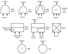
Figure 1: RFT elements

The intuition about the behavior of each gate is as follows. An AND gate fails whenever all its inputs fail, and gets repaired (stop failing) when at least one of its inputs is repaired. An OR gate fails whenever at least one of its inputs fails and is repaired when all of its inputs are repaired. A $k/n$ VOTING gate fails whenever at least $k$ of its $n$ inputs fail and stops failing if at most $k-1$ of its inputs remain failing. A PAND gate fails whenever its inputs fail from left to right, inducing an order on the failure occurrence, and it is repaired if the last input is repaired. A functional dependency gate (FDEP) has $n+1$ inputs. The fail signal of one of its inputs (the triggering one) makes all the other inputs inaccessible to the rest of the system. Note that the dependent inputs do not necessarily fail, and they will be accessible again as soon as the triggering component is repaired (note the difference with [6, 31] where dependent BEs do fail). In fact this gate can be easily replaced by a system of OR gates [34]. A spare basic element (SBE) is a special case of BE which can be enabled and disabled, and can be used as spare parts for other BEs through spare gates. A same SBE can be shared by several spare gates, and different sharing policies are introduced for this purpose. A spare gate (SG) allows to replace a basic element by one of several spare basic elements in case it fails. Each spare gate has a main input and $n$ spare parts inputs. The main input can only be a BE. The spare inputs can only be SBEs. As soon as the main input fails, the SG uses its own policy to ask for the replacement by one of its spare inputs. The SG will fail whenever it does not obtain a replacement, and will signal repair whenever the main input gets repaired or a spare input is obtained. If an in-use replacement fails the SG will look for a new one. If the main input is repaired, the SG will free the acquired spare input, in case there is one. A repair box (RBOX) is the unit in charge of managing the repairing of failed BEs and SBEs. They have $n$ inputs, which are the elements administered for repairing, and a dummy output. A RBOX policy determines in which order the failing elements will be repaired. Also notice that a RBOX can only repair one of its inputs at a time, while the rest of its failing inputs are waiting for repair.

3 Input/Output Stochastic Automata

Input/Output Stochastic Automata [15, 17] is a modelling formalism tailored to model stochastic systems for the purpose of simulation. IOSA combine continuous probability jumps from Stochastic Automata, with discrete event synchronisation for a compositional style of modelling. IOSAs use continuous random variables to control and observe the passage of time. These variables, called clocks, are set to a value according to their associated probability distribution, and, as time evolves, count down all at the same rate until they reach the value of zero. Clocks control the moments when actions are taken, and thus allow to model systems where events occur at random continuous time stamps. Output and input transitions can be used to synchronize and communicate between different IOSAs. Output transitions are autonomous, while inputs occurrence depends on synchronisation with outputs. A transversal classification for actions allows to mark them as urgent or non urgent. While a non-urgent output is controlled by the expiration of clocks (i.e., clocks reaching the value zero), an urgent output action is taken as soon as the state in which it is enabled is reached. Though an IOSA may be non-deterministic, [17] provides a set of sufficient conditions that guarantee weak determinism (i.e. only spurious non-determinism is present). Furthermore, such conditions can be checked with a polynomial algorithm on the components of the model.

Definition 1

An input/output stochastic automaton with urgency (IOSA) is a structure $(\mathcal{S},\mathcal{A},\mathcal{C},\xrightarrow{\,{}\,},C_{0},s_{0})$, where $\mathcal{S}$ is a (denumerable) set of states, $\mathcal{A}$ is a (denumerable) set of labels partitioned into disjoint sets of input labels $\mathcal{A}^{\mathsf{i}}$ and output labels $\mathcal{A}^{\mathsf{o}}$, from which a subset $\mathcal{A}^{\mathsf{u}}\subseteq\mathcal{A}$ is marked as urgent, $\mathcal{C}$ is a (finite) set of clocks such that each $x\in\mathcal{C}$ has an associated continuous probability measure $\mu_{x}$ on $\mathbb{R}$ s.t. $\mu_{x}(\mathbb{R}_{>0})=1$, ${\xrightarrow{\,{}\,}}\subseteq\mathcal{S}\times\mathcal{C}\times\mathcal{A}\times\mathcal{C}\times S$ is a transition function, $C_{0}$ is the set of clocks that are initialized in the initial state, and $s_{0}\in\mathcal{S}$ is the initial state. In addition it should satisfy the following constraints:

1. If $s\xrightarrow{\,{C,\mathit{a},C^{\prime}}\,}s^{\prime}$ and $\mathit{a}\in\mathcal{A}^{\mathsf{i}}\cup\mathcal{A}^{\mathsf{u}}$, then $C=\varnothing$.

2. If $s\xrightarrow{\,{C,\mathit{a},C^{\prime}}\,}s^{\prime}$ and $\mathit{a}\in\mathcal{A}^{\mathsf{o}}\setminus\mathcal{A}^{\mathsf{u}}$, then $C$ is a singleton set.

3. If $s\xrightarrow{\,{\{x\},\mathit{a}_{1},C_{1}}\,}s_{1}$ and $s\xrightarrow{\,{\{x\},\mathit{a}_{2},C_{2}}\,}s_{2}$ then $\mathit{a}_{1}=\mathit{a}_{2}$, $C_{1}=C_{2}$ and $s_{1}=s_{2}$.

4. For every $\mathit{a}\in\mathcal{A}^{\mathsf{i}}$ and state $s$, there exists a transition $s\xrightarrow{\,{\varnothing,\mathit{a},C}\,}s^{\prime}$.

5. For every $\mathit{a}\in\mathcal{A}^{\mathsf{i}}$, if $s\xrightarrow{\,{\varnothing,\mathit{a},C_{1}^{\prime}}\,}s_{1}$ and $s\xrightarrow{\,{\varnothing,\mathit{a},C_{2}^{\prime}}\,}s_{2}$, $C_{1}^{\prime}=C_{2}^{\prime}$ and $s_{1}=s_{2}$.

6. There exists a function $\mathit{active}:\mathcal{S}\rightarrow 2^{\mathcal{C}}$ such that: (i) $\mathit{active}(s_{0})\subseteq C_{0}$, (ii) $\mathit{enabling}(s)\subseteq\mathit{active}(s)$, (iii) if $s$ is stable, $\mathit{active}(s)=\mathit{enabling}(s)$, and (iv) if $t\xrightarrow{\,{C,a,C^{\prime}}\,}s$ then $\mathit{active}(s)\subseteq(\mathit{active}(t)\setminus C)\cup C^{\prime}$.

where $\mathit{enabling}(s)=\{y\mid s\xrightarrow{\,{\{y\},\_,\_}\,}\_\}$, and $s$ is stable if there is no $a\in\mathcal{A}^{\mathsf{u}}\cap\mathcal{A}^{\mathsf{o}}$ such that $s\xrightarrow{\,{\varnothing,a,\_}\,}\_$. ($\_$ indicates the existential quantification of a parameter.)

Restrictions (a) to (f) are there to ensure that at most one non-urgent output action is enabled at a time. If in addition the IOSA is closed (i.e., all communications have been resolved and hence the set of inputs is empty) and all its urgent actions are confluent (in the sense of [26], see also Def. 5) it turns out all the non-determinism is spurious and does not alter the stochastic behavior (i.e. regardless of how non-determinism is resolved, the stochastic properties remain the same) [15, 17]. We call this property weak determinism.

IOSAs are closed under parallel composition which is defined according to rules in Table 1. In order to avoid unintended behavior, the component IOSAs are requested to be compatible, that is, they should not share output actions nor clocks, and be consistent with respect to urgent actions.

Table 1: Parallel composition on IOSA

$$\frac{s_{1}\xrightarrow{\,{C,\mathit{a},C^{\prime}}\,}_{1}s_{1}^{\prime}}{s_{1}||s_{2}\xrightarrow{\,{C,\mathit{a},C^{\prime}}\,}s_{1}^{\prime}||s_{2}}\ \mathit{a}\in\mathcal{A}_{1}{\setminus}\mathcal{A}_{2}$$ (1)

$$\frac{s_{2}\xrightarrow{\,{C,\mathit{a},C^{\prime}}\,}_{2}s_{2}^{\prime}}{s_{1}||s_{2}\xrightarrow{\,{C,\mathit{a},C^{\prime}}\,}s_{1}||s_{2}^{\prime}}\ \mathit{a}\in\mathcal{A}_{2}{\setminus}\mathcal{A}_{1}$$ (2)

$$\frac{s_{1}\xrightarrow{\,{C_{1},\mathit{a},C^{\prime}_{1}}\,}_{1}s_{1}^{\prime}\quad s_{2}\xrightarrow{\,{C_{2},\mathit{a},C^{\prime}_{2}}\,}_{2}s_{2}^{\prime}}{s_{1}||s_{2}\xrightarrow{\,{C_{1}\cup C_{2},\mathit{a},C^{\prime}_{1}\cup C^{\prime}_{2}}\,}s_{1}^{\prime}||s_{2}^{\prime}}\ \mathit{a}\in\mathcal{A}_{1}{\cap}\mathcal{A}_{2}$$ (3)

4 IOSA symbolic language

⬇

1module BE

2 fc, rc : clock;

3 inform : [0..2] init 0;

4 broken : [0..2] init 0;

5

6 [fl!] broken=0 @ fc -> (inform’=1) & (broken’=1);

7 [r??] broken=1 -> (broken’=2) & (rc’=$\gamma$);

8 [up!] broken=2 @ rc -> (inform’=2) &

9 (broken’=0) & (fc’=$\mu$);

10

11 [f!!] inform=1 -> (inform’=0);

12 [u!!] inform=2 -> (inform’=0);

13endmodule

Figure 2: Basic Element IOSA symbolic model.

We present a symbolic language to describe an IOSA model. This language is the input language of the tool FIG [12, 10] and has some strong resemblance with the PRISM modelling language [23]. IOSAs compositional style of modelling is also reflected in the language, where each component is modeled separately by what we call a module. A module is composed of a set of variables, whose valuation represent the actual state of the component, a set of clocks corresponding to the enabling clocks for non urgent transitions, and a set of transitions which symbolically describe the possible jumps between states (changes of valuations and resetting of clocks). Fig. 2 models a basic element as an example. Variables can be of integer (with finite range) or boolean type. As we will see later, also arrays can be defined as variables. An initial value for each variable is determined after the keyword init. Clocks measures are defined at the transitions where they are reset. A transition is described by the name of the action which takes place, a guard that defines the origin states, an enabling clock (only for the case of non-urgent output transitions), a condition describing the target states, and the set of clocks to be reset. A quick overview of Fig. 2 will help to further understand our symbolic language: Two clocks, fc and rc, are defined at line $2$. These clocks will be used as enabling clocks for transitions at lines $6$ and $8$, and reset on transitions at lines $7$ and $9$ where $\gamma$ and $\mu$ are the distribution associated with rc and fc, respectively. Lines $3$ and $4$ define variables inform and broken, both of integer type ranging between $0$ and $2$, and initialized with value $0$. Line $6$ defines a set of non-urgent output transitions, which produce the output action fl. More precisely, this line defines the set of non-urgent transitions $s\xrightarrow{\,{\{\text{\small fc}\},\text{\small fl!},\varnothing}\,}s^{\prime}$, where $s$ meets the condition broken=0, and $s^{\prime}$ is the result of changing the values of variables inform and broken to 1 while other variables remain with the same values as those in state $s$. The @ symbol precedes the enabling clock for the transition while the -> symbol distinguishes between conditions for the origin state and the target state. The conditions on the target state are expressed as assignments to the next values of the variables, indicated with an apostrophe. Line $7$ defines an urgent input transition with label r. The double question marks after the name indicates that it describes urgent input transitions. Urgent output transition are indicated with double exclamation marks (!!), non urgent input transitions with a single question mark, and non-urgent output transitions with a single exclamation mark. At the end of line $7$ we find the reset of the clock rc to a value from a probability distribution $\gamma$. This line then defines transitions $s\xrightarrow{\,{\varnothing,\text{\small r??},\{\text{\small rc}\}}\,}s^{\prime}$, where $s$ meets with condition broken=1 and $s^{\prime}$ is identical to $s$ except for variable broken which has value 2. At line $11$, an urgent output transition is defined, indicating the failure of this component through action f!!. We will usually use these urgent transitions to synchronize and communicate with other modules.

The text of Fig. 2 is tacitly completed with self-loops with all inputs in all constraints that are not explicitly written. For example, in Fig. 2, the line “[r??] broken != 1 -> ;” is assumed to exist.

5 A formal syntax for RFT and its semantics

In this section we present a formal definition of the RFT similar to those of [5, 7] along with its semantics given in terms of IOSA. Each element of a RFT is characterized by a tuple consisting of its type, its arity (i.e. number of inputs), and possibly other parameters like probability distributions for fail and repair events in a BE.

Definition 2

Let $n,m,k\in\mathbb{N}^{+}$, and let $\mu$, $\nu$ and $\gamma$ be continuous probability distributions. We define the set $\mathcal{E}$ of elements of a RFT to be composed of the following tuples:

• $(\mathsf{be},0,\mu,\gamma)$ and $(\mathsf{sbe},0,\mu,\nu,\gamma)$, which represents basic and spare basic elements, with no inputs, with an active failure distribution $\mu$, a dormant failure distribution $\nu$, and a repair distribution $\gamma$.

• $(\and,n)$, $(\mathsf{or},n)$ and $(\mathsf{pand},n)$, which represent AND, OR and PAND gates with $n$ inputs, respectively,

• $(\mathsf{vot},n,k)$, which represent a $k$ from $n$ voting gate,

• $(\mathsf{fdep},n)$, which represents a functional dependency gate, with $1$ trigger input and $n-1$ dependent ones. By convention the first input is the triggering one.

• $(\mathsf{sg},n)$, which represents a SPARE gate with one main input and $n-1$ spare inputs. By convention the first input is the main one.

• $(\mathsf{rbox},n)$, which represents a RBOX element for $n$ BEs (or SBEs).

A RFT is a directed acyclic graph, for which every vertex $v$ is labeled with an element $\textrm{$l$}(v)\in\mathcal{E}$. An edge from $v$ to $w$ means that the output of $v$ is connected to an input of $w$. Since the order of the inputs is relevant, we give them in terms of a list $i(w)$ instead of a set. Similarly, $si(v)$ will list all the spare gates to which a spare basic element $v$ is connected as an input. Let $\textrm{{t}}(v)$ indicate the type of $v$. That is, $\textrm{{t}}(v)$ is the first projection of $\textrm{$l$}(v)$. Let $\mathcal{\#}(v)$ indicate the number of inputs of $v$, that is, it is the second projection $\textrm{$l$}(v)$.

Definition 3

A repair fault tree is a four-tuple $T=(V,i,si,\textrm{$l$})$, where $V$ is a set of vertices, $\textrm{$l$}\colon V\rightarrow\mathcal{E}$ is a function labeling each vertex with a RFT element, $i\colon V\rightarrow V^{*}$ is a function assigning $\mathcal{\#}(v)$ inputs to each element $v$ in $V$, and $si\colon V\rightarrow V^{*}$ which indicate which spare gates manage each spare BE. The set of edges $\text{E}=\{(v,w)\in V^{2}\mid\exists j\cdot v=(i(w))[j]\}$ is the set of pairs $(v,w)$ such that $v$ is an input of $w$. If such an edge exists, we will say that $v$ is connected to $w$ and $w$ to $v$. In addition, a RFT $T$ should satisfy the following conditions:

• The tuple $(V,\text{E})$ is a directed acyclic graph (DAG).

• $T$ has a unique top element, i.e. a unique element whose non dummy output is not connected to another gate. That is, there is a unique vertex $v\in V$ such that for all $w\in V$, $(v,w)\notin E$ and $\textrm{{t}}(v)\neq\mathsf{fdep},\mathsf{rbox}$.

• An output can not be more than once the input of a same gate. That is, for all $1\leq j,k\leq|i(w)|$ with $i(w)[j]=i(w)[k]$, we have $j=k$.

• Since FDEP and RBOX outputs are dummy, if $(v,w)\in E$ then $\textrm{{t}}(v)\notin\{\mathsf{fdep},\mathsf{rbox}\}$.

• The inputs of a repair box can only be basic elements. I.e., if $(v,w)\in E$ and $\textrm{{t}}(w)=\mathsf{rbox}$ then either $\textrm{{t}}(v)=\mathsf{be}$ or $\textrm{{t}}(v)=\mathsf{sbe}$.

• Each (spare) basic element can be connected to a single RBOX. I.e., if $(v,w)\in E$ and $(v,w^{\prime})\in E$ and $\textrm{{t}}(w)=\textrm{{t}}(w^{\prime})=\mathsf{rbox}$, then $w=w^{\prime}$.

• The spare inputs of a spare gate can only be spare basic elements, while its main input can only be a basic element. I.e., if $(v,w)\in E$ and $\textrm{{t}}(w)=\mathsf{sg}$ then $\textrm{{t}}(i(v)[0])=\mathsf{be}$ and for $j>0,\textrm{{t}}(i(v)[j])=\mathsf{sbe}$. Furthermore, a spare basic element can only be connected to a spare gate or a RBOX, i.e., if $(v,w)\in E$ and $\textrm{{t}}(v)=\mathsf{sbe}$ then $\textrm{{t}}(w)\in\{\mathsf{sg},\mathsf{rbox}\}$.

• A spare basic element is an input of a spare gate, if and only if that spare gate is spare input of the spare basic element, i.e. for $v$ and $v^{\prime}$ such that $\textrm{$l$}(v^{\prime})=(\mathsf{sbe},0,\mu,\nu,\gamma)$ and $\textrm{$l$}(v)=(\mathsf{sg},n)$, $(v^{\prime},v)\in E$ if and only if there exists $j$ such that $v=si(v^{\prime})[j]$.

• A basic element can be connected to at most one spare gate, i.e. if $(v,w)\in E$ and $(v,w^{\prime})\in E$ with $\textrm{{t}}(w)=\textrm{{t}}(w^{\prime})=\mathsf{sg}$ and $\textrm{{t}}(v)=\mathsf{be}$ then $w=w^{\prime}$.

• If a basic element is connected to a spare gate then it can not be connected to a FDEP gate, i.e. if $(v,w)\in E$ and $\textrm{{t}}(v)=\mathsf{be}$ and $\textrm{{t}}(w^{\prime})=\mathsf{sg}$, then there is no $(v,w^{\prime})\in E$ such that $\textrm{{t}}(w^{\prime})=\mathsf{fdep}$.

In the following, we present a parametric semantics for RFT elements. This will be used later to obtain the semantics for each vertex in a given RFT, and the consequent semantics of the full model as a parallel composition of its components. In this section, we only give the semantics for BEs, AND gates, OR gates, PAND gates, and RBOX. Remember that FDEP can be replaced by OR gates. Similarly, voting gates can be modeled by a series of AND and OR gates (although a simpler model can be found in Appendix 0.D). In the design of the IOSA modules we should take into account the communication of each element of a RFT with its children and parents. For instance a basic element has to communicate its failure and repair to those gates for which it is an input. Similarly, a RBOX has to communicate to its inputs a start repairing signal. In order to do so, the semantics of each element will be given by a function, which takes actions as parameters.

⬇

1module AND

2 informf: bool init false;

3 informu: bool init false;

4 count: [0..2] init 0;

5

6 [f₁??] count=1 -> (count’=2) & (informf’=true);

7 [f₁??] count=0 -> (count’=1);

8 [f₁??] count=2 -> ;

9 [f₂??] count=1 -> (count’=2) & (informf’=true);

10 [f₂??] count=0 -> (count’=1);

11 [f₂??] count=2 -> ;

12

13 [u₁??] count=2 -> (count’=1) & (informu’=true);

14 [u₁??] count=1 -> (count’=0);

15 [u₁??] count=0 -> ;

16 [u₂??] count=2 -> (count’=1) & (informu’=true);

17 [u₂??] count=1 -> (count’=0);

18 [u₂??] count=0 -> ;

19

20 [f!!] informf & count=2 -> (informf’=false);

21 [u!!] informu & count!=2 -> (informu’=false);

22endmodule

Figure 3: AND gate IOSA symbolic model.

For a BE element $e\in\mathcal{E}$, its semantics is a function $[\![e]\!]:\mathcal{A}^{5}\rightarrow IOSA$, where $[\![(\mathsf{be},0,\mu,\gamma)]\!](\textsf{{\small fl}},\textsf{{\small up}},\textsf{{\small f}},\textsf{{\small u}},\textsf{{\small r}})$ results in the IOSA of Fig. 2. The state of a basic element is defined by the fail clock fc, the repair clock rc, a variable signal that indicates when to signal the failure or repair, and variable broken to distinguish between broken and normal states. A basic element fails when clock fc expires (line 6) and immediately informs it with the urgent signal f!! at line 11. As soon as the repair begins by the corresponding connected repair box (line 7), clock rc is set. When it expires, the component becomes repaired. Hence, fc is set again at line 8, and the repair is signaled with urgent action u!! at line 11. At the starting state of an IOSA module all its clocks are set randomly according to their associated distributions. Thus, rc is set at the initial state and could eventually expire without having been set by a repair transition. This is why we have to distinguish between cases when the BE is being repaired (broken=2) from when it is not.

For an AND gate element with two inputs, its semantics is a function $[\![e]\!]:\mathcal{A}^{6}\rightarrow IOSA$, where $[\![(\and,2)]\!](\textsf{{\small f}},\textsf{{\small u}},\textsf{{\small f${}_{1}$}},\textsf{{\small u${}_{1}$}},\textsf{{\small f${}_{2}$}},\textsf{{\small u${}_{2}$}})$ results in the IOSA in Fig. 3. At lines 6 to 11, the AND gate gets informed of the failure of either of its inputs. Upon failure of some input, we distinguish between the case where the other input has already failed (count=1) and the case where it has not (count=0). In the first case the AND gate has to move to a failure state, for which we set the informf variable in order to enable the signaling of failure at line 20. Furthermore in both cases we increase the value of count so that we take note of the failure of an input. A similar reasoning is done for the case of the repairing of an input at lines 13 to 18. In this case we have to set the module to signal a repair when an input gets repaired at a state where both inputs were failing (lines 13 and 16), by enabling transition at line 21. From now on, we omit writing down self loops originated by IOSA’s input enabledness, such as lines $8,11,15$ and $18$ as they are assumed to be there. Nevertheless, we remark that it is necessary to take them into account when analyzing confluence in the next section. The semantics for an OR gate is similar to the AND gate and can be found in Appendix 0.B.

The semantics of a $n$ inputs repair box with priority policy, is a function $[\![(\mathsf{rbox},n)]\!]:\mathcal{A}^{3*n}\rightarrow IOSA$, where $[\![(\mathsf{rbox},n)]\!](\textsf{{\small fl}}_{0},\textsf{{\small up}}_{0},\textsf{{\small r}}_{0},...,\textsf{{\small fl}}_{n-1},\textsf{{\small up}}_{n-1},$ $\textsf{{\small r}}_{n-1})$ results in the IOSA of Fig. 4. The RBOX with priority uses the array broken[n]

⬇

1module RBOX

2 broken[n]: bool init false;

3 busy: bool init false;

4

5 [fl₀?] -> (broken[0]’=true);

6 ...

7 [fl_n-1?] -> (broken[n-1]’=true);

8

9 [r₀!!] !busy & broken[0] -> (busy’=true);

10 ...

11 [r_n-1!!] !busy & broken[n-1] & !broken[n-2]

12 & ... & !broken[0] -> (busy’=true);

13

14 [up₀?] -> (broken[0]’=false) & (busy’=false);

15 ...

16 [up_n-1?] -> (broken[n-1]’=false) & (busy’=false);

17endmodule

Figure 4: RBOX with priority policy

to keep track of failed inputs, updating it when it receives their fail signals (lines 5 to 7) and up signals (lines 13 to 15). At the same time, when not busy, it sends repair signals to broken inputs (lines 9 to 12). Guards ensure the priority order for repairing. Note that instead of listening to the urgent output signals of the input BEs, it listens for the non-urgent actions of the transitions that trigger the failure or repair. This is done with the only purpose of facilitating the confluence analysis over this module. Other types of repair boxes can be modeled, taking into account different repairing policies. (see App. 0.C).

The semantics of a Priority AND gate with $2$ inputs is defined by $[\![(\mathsf{pand},2)]\!]:\mathcal{A}^{6}\rightarrow IOSA$, where $[\![(\mathsf{pand},2)]\!](\textsf{{\small f}},\textsf{{\small u}},\textsf{{\small f}}_{0},\textsf{{\small u}}_{0},\textsf{{\small f}}_{1},\textsf{{\small u}}_{1})$ results in the IOSA of Fig. 5. PAND gates fail only when their inputs fail from left to right. This allows to condition the failure of a system not only to the failure of the subsystems but also to the ordering in which they fail. Notice that an $n$ inputs PAND gate is simply a syntax sugar for a system of $n-1$ two-input PAND gates connected in cascade. Literature is not always clear or even disagrees on what should be the behavior of the PAND gate in case both inputs fail at the same time [24, 14]. This situation arises in some constructions with AND and OR gates, or when the inputs of a PAND gate are connected to the a same FDEP (see Fig. 6). Some proposals disallow these situations and discard them on early syntactic checks [31].

⬇

1module PAND

2

3 f1: bool init false;

4 f2: bool init false;

5 st: [0..4] init 0; \\ up, inform fail, failed,

6 inform up, unbreakable

7

8 [_?] st=0 & f1 & !f0 -> (st’=4);

9

10 [f₀??] st=0 & !f0 & !f1-> (f0’=true);

11 [f₀??] st=0 & !f0 & f1 -> (st’=1) & (f0’=true);

12 [f₀??] st!=0 & !f0 -> (f0’=true);

13 [f₀??] f0 -> ;

14

15 [f₁??] st=0 & !f0 & !f1 -> (f1’=true);

16 [f₁??] st=0 & f0 & !f1 -> (st’=1) & (f1’=true);

17 [f₁??] st=3 & !f1 -> (st’=2) & (f1’=true);

18 [f₁??] (st==1|st==2|st=4) & !f1 -> (f1’=true);

19 [f₁??] f1 -> ;

20

21 [u₀??] st!=1 & f0 -> (f0’=false);

22 [u₀??] st=1 & f0 -> (st’=0) & (f0’=false);

23 [u₀??] !f0 -> ;

24

25 [u₁??] (st=0|st=3) & f1 -> (f1’=false);

26 [u₁??] (st=1|st=4) & f1 -> (st’=0) & (f1’=false);

27 [u₁??] st=2 & f1 -> (st’=3) & (f1’=false);

28

29 [f!!] st=1 -> (st’=2);

30 [u!!] st=3 -> (st’=0);

31

32endmodule

Figure 5: PAND gate.

Some others assume a non-deterministic situation and find it important to analyze scenarios where the behavior is in fact unknown [5]. Other works decided that the PAND gate does not fail unless its inputs break strictly from left to right [6, 4]. Some others state that PAND gates also fail when both their inputs fail at the same time [14, 9, 8]. We opted for this last case, so the gates needs to be able to identify if time has passed between the occurrence of the failures, and act consequently. In the particular case where no time passes between the failure of the inputs, we consider that the order in which the dependent BEs fail does not really matter and thus the non-determinism is spurious. To identify if time has passed between the occurrence of the input failures, the model listens to any output actions, which indicate that a clock has expired.

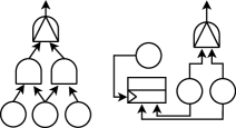
Figure 6: Spurious non-determinism.

This is done by a special input action at line 8, which synchronizes with all non-urgent outputs, regardless the name of the action. Notice that there is only one scenario that we want to rule out, which is when the second input fails and then time passes without the first input failing too. This is in fact the case described by the guard of line 8. Furthermore, this transition moves to the ‘unbreakable’ state, from which it can only go back when input 1 is fixed. In consequence, the failure of the gate occurs either if both inputs fail at the same time or if the first input fails, then time passes, and then the second input fails.

The semantics of a RFT is that of the parallel composition of the semantics of its components, being conveniently synchronized.

Definition 4

Given a RFT $T=(V,i,si,\textrm{$l$})$ we define the semantics of $T$ as $[\![T]\!]=||_{v\in V}[\![v]\!]$ where $[\![v]\!]$ is defined by:

$$[\![v]\!]=\begin{cases}[\![\textrm{$l$}(v)]\!](\text{\rm{{\small fl}}}_{v},\text{\rm{{\small up}}}_{v},\text{\rm{{\small f}}}_{v},\text{\rm{{\small u}}}_{v},\text{\rm{{\small r}}}_{v})&\text{if }\textrm{$l$}(v)=(\mathsf{be},0,\mu,\gamma)\\ [\![\textrm{$l$}(v)]\!](\text{\rm{{\small f}}}_{v},\text{\rm{{\small u}}}_{v},\text{\rm{{\small f}}}_{i(v)[0]},\text{\rm{{\small u}}}_{i(v)[0]},...,\text{\rm{{\small f}}}_{i(v)[n-1]},\text{\rm{{\small u}}}_{i(v)[n-1]})\\ &\text{if }\textrm{$l$}(v)\in\{(\and,n),(\mathsf{or},n)\}\\ [\![\textrm{$l$}(v)]\!](\text{\rm{{\small f}}}_{v},\text{\rm{{\small u}}}_{v},\text{\rm{{\small f}}}_{i(v)[0]},\text{\rm{{\small u}}}_{i(v)[0]},\text{\rm{{\small f}}}_{i(v)[1]},\text{\rm{{\small u}}}_{i(v)[1]})&\text{if }\textrm{$l$}(v)=(\mathsf{pand},2)\\ [\![\textrm{$l$}(v)]\!](\text{\rm{{\small fl}}}_{i(v)[0]},\text{\rm{{\small up}}}_{i(v)[0]},\text{\rm{{\small r}}}_{i(v)[0]},...,\text{\rm{{\small fl}}}_{i(v)[n-1]},\text{\rm{{\small up}}}_{i(v)[n-1]},\text{\rm{{\small r}}}_{i(v)[n-1]})\\ &\text{if }\textrm{$l$}(v)=(\mathsf{rbox},n)\end{cases}$$

In Section 7, we extend the semantics to spare gates and spare basic elements.

6 RFTs are weakly deterministic

In this section we show that RFTs composed only by BEs, AND gates, OR gates, PAND gates, and RBOX, are weakly deterministic. Since voting and FDEP gates can be constructed using OR and AND gates, the result extends to these gates. Results in this section rely heavily on results about weak determinism on IOSA proven in [17]. Therefore, we first summarize the essentials of [17] for this paper.

Definition 5

An IOSA is confluent if for all pair of urgent actions $a$ and $b$, and for every (reachable) state $s$, it satisfies that, if $s\xrightarrow{\,{\varnothing,a,C_{1}}\,}s_{1}$ and $s\xrightarrow{\,{\varnothing,b,C_{2}}\,}s_{2}$, then there is a state $s_{3}$ such that $s_{2}\xrightarrow{\,{\varnothing,a,C_{1}}\,}s_{3}$ and $s_{1}\xrightarrow{\,{\varnothing,b,C_{2}}\,}s_{3}$.

Note that, according to this definition, regardless the order of the confluent transitions, the same state is reached. This non-determinism is spurious in the sense that it does not alter the stochastic properties of the given IOSA, regardless the manner it is solved. Since non-determinism can only arise on urgent actions, we say that a closed IOSA is weakly deterministic if all its urgent actions are confluent. In [17], we provided sufficient conditions to ensure that a closed IOSA is weakly deterministic. This is stated in Theorem 6.1 below which requires the following definition.

Definition 6

Given an IOSA $\mathcal{I}$ with state space $\mathcal{S}$ and actions $\mathcal{A}$, we distinguish the following sets of actions:

• A set of urgent output actions $B\subseteq\mathcal{A}^{\mathsf{o}}\cap\mathcal{A}^{\mathsf{u}}$ is initial if each $b\in B$ is enabled in $s_{0}$, i.e. if for each $b\in B$ there is a state $s\in\mathcal{S}$ and $C\subseteq\mathcal{C}$, such that $s_{0}\xrightarrow{\,{\varnothing,b,C}\,}s$.

• We say that a set $B\subseteq\mathcal{A}^{\mathsf{o}}\cap\mathcal{A}^{\mathsf{u}}$ of output urgent actions is spontaneously enabled by $b\in\mathcal{A}\setminus\mathcal{A}^{\mathsf{u}}$ if there are stochastically reachable states $s,s^{\prime}\in\mathcal{S}$ (a state is stochastically reachable if there is a path in the IOSA from the initial state that reaches such state with probability greater than zero) such that $s$ is stable, $s\xrightarrow{\,{\_,b,\_}\,}s^{\prime}$, and all actions in $B$ are enabled in $s^{\prime}$.

• Let $\mathit{a}\in\mathcal{A}^{\mathsf{u}}$ and $\mathit{b}\in\mathcal{A}^{\mathsf{o}}\cap\mathcal{A}^{\mathsf{u}}$. We say that $\mathit{a}$ triggers $\mathit{b}$ if there are stochastically reachable states $s_{1},s_{2},s_{3}\in\mathcal{S}$ such that: $s_{1}\xrightarrow{\,{\_,a,\_}\,}s_{2}$, $s_{2}\xrightarrow{\,{\_,b,\_}\,}s_{3}$, and, if $\mathit{a}\neq\mathit{b}$, then there is no outgoing transition from $s_{1}$ labeled with $b$. The set $\{(a,b)\mid a\text{ triggers }b\}$ is called the triggering relation.

The approximate indirect triggering relation of a composite IOSA is defined as the reflexive transitive closure of the union of the triggering relations of its components. The following theorem from [17], gives necessary conditions for a closed IOSA not to be confluent. As a consequence, it provides sufficient conditions for a closed IOSA to be weakly deterministic.

Theorem 6.1

Given a closed composite IOSA $\mathcal{I}=\left(\mathcal{I}_{1}||\ldots||\mathcal{I}_{n}\right)$ with actions $\mathcal{A}$, if $\mathcal{I}$ is not confluent then there exist a pair of urgent actions $\mathit{a},\mathit{b}\in\mathcal{A}^{\mathsf{u}}$ such that

1. one of the components is not confluent with respect to $\mathit{a}$ and $\mathit{b}$,

2. there are actions $c$ and $d$ that approximately indirectly trigger both $a$ and $b$, respectively, and

3. one of the following hold: (i) $c$and $d$ are initial actions, or (ii) there exists an action $e$ and possible empty sets $B_{1}$ to $B_{n}$ spontaneously enabled by $e$ in $\mathcal{I}_{1}$ to $\mathcal{I}_{n}$ respectively, such that $c$ and $d$ are in $\bigcup_{i=1}^{n}B_{i}$.

In the following, we prove accessory propositions to eventually prove, using Theorem 6.1, that the IOSA defined by a RFT is weakly deterministic.

Proposition 1

Let $T$ be a RFT. $[\![T]\!]$ has no initially enabled actions. Moreover, the only spontaneous sets of actions are singletons of the form $\{\text{\rm\text{\small f}}_{v}\}$ and $\{\text{\rm\text{\small u}}_{v}$}, for $\textrm{{t}}(\textrm{$l$}(v))=\mathsf{be}$, which are spontaneously enabled by $\text{\rm\text{\small fl}}_{v}$ and $\text{\rm\text{\small up}}_{v}$, respectively.

Proof

As a consequence of [17], the initially enabled actions of $[\![T]\!]$ are contained in the union of the sets of initially enabled actions of its components $[\![v]\!]$, $v\in V$, and the spontaneously enabled actions of $[\![T]\!]$ are contained in the union of the spontaneously enabled sets of $[\![v]\!]$. It is direct to see that, for any element $e\in\mathcal{E}$, none of the urgent outputs are enabled at the initial state of $[\![e]\!]$, since their guards are initially false. Furthermore, the only non-urgent output transition in our models are at lines 6 and 8 of the BE (Fig. 2). Let $v\in V$ such that $\textrm{{t}}(v)=\mathsf{be}$. Then, after taking transition at line 6 the only urgent output enabled is $\text{\small f}_{v}$ (on the instance $[\![v]\!]$), while after taking transition at line 8 the only one is $\text{\small u}_{v}$, and thus these are the only possible spontaneous enabled actions. ∎

Proposition 2

Let $T$ be a RFT. The only possible pairs of non-confluent actions in $[\![T]\!]$ are $\{(\text{\rm{{\small f}}}_{v},\text{\rm{{\small u}}}_{v^{\prime}})\mid v,v^{\prime}\in i(w),t(w)\in\{\and,\mathsf{or},\mathsf{pand}\}\}\cup\{(\text{\rm{{\small f}}}_{w},\text{\rm{{\small u}}}_{v}),(\text{\rm{{\small u}}}_{w},\text{\rm{{\small f}}}_{v})\mid v\in i(w),t(w)\in\{\and,\mathsf{or}\}\}$.

Proof

The proof of this Proposition follows an exhaustive check over each urgent transition of each model, in order to single out any non-confluent situation, and can be found at Appendix 0.E

Proposition 3

Let $T$ be a RFT. For each $v\in V$, the triggering relation of $[\![v]\!]$ is given by:

• $\{\}$, if $\textrm{$l$}(v)\in\{(\mathsf{be},0,\mu,\gamma),(\mathsf{rbox},n)\}$,

• $\{(\text{\rm{{\small f}}}_{w},\text{\rm{{\small f}}}_{v})\mid w\in i(v)\}\cup\{(\text{\rm{{\small u}}}_{w},\text{\rm{{\small u}}}_{v})\mid w\in i(v)\}$, if $\textrm{$l$}(v)\in\{(\and,n),(\mathsf{or},n)\}$, and

• $\{(\text{\rm{{\small u}}}_{w},\text{\rm{{\small u}}}_{v})\mid w=i(v)[1]\}\cup\{(\text{\rm{{\small f}}}_{w},\text{\rm{{\small f}}}_{v})\mid w\in i(v)\}$, if $\textrm{$l$}(v)=(\mathsf{pand},2)$.

Proof (sketch)

It sufficies to make a satisfiability analysis over guards and postconditions of each pair $(t_{a},t_{b})$ with $t_{b}$ an output urgent symbolic transition and $t_{a}$ any urgent symbolic transition, taking into account only reachable states. ∎

Theorem 6.2

Let $T$ be a RFT. Then $[\![T]\!]$ is weakly deterministic.

Proof

We look for $a,b,c,d$ and $e$ as well as sets $B_{i}$ with $i=1\dots n$ as Theorem 6.1 suggests. Since Prop. 1 ensures that there are no initially enabled actions in $[\![T]\!]$, $c$ and $d$ should be spontaneously enabled actions. By the same proposition either $e$ is of the form $\text{\small fl}_{v}$ for some $v$ and then $\bigcup_{i=1}^{1}B_{i}=B_{1}=\{\text{\small f}_{v}\}$, or $e$ is of the form $\text{\small up}_{v}$ for some $v$ and then $\bigcup_{i=1}^{1}B_{i}=B_{1}=\{\text{\small u}_{v}\}$. In the first case, we get $c=d=\text{\small f}_{v}$ for some $v$, and in the second case $c=d=\text{\small u}_{v}$. Furthermore, by Prop. 2, either $a$ is of the form $\textsf{{\small f}}_{w}$ for some $w$ and $b$ is of the form $\textsf{{\small u}}_{w^{\prime}}$ for some $w^{\prime}$ or the other way around. As shown by Prop. 3, fail actions ($\textsf{{\small f}}_{v}$ for some $v$) only trigger fail actions and up actions ($\textsf{{\small u}}_{v}$ for some $v$) only trigger up actions, thus it is impossible that $c$ and $d$ indirectly trigger $a$ and $b$ respectively. Therefore, it is not possible to find actions $a$, $b$, $c$, $d$, and $e$ satisfying conditions 1 to 3 in Theorem 6.1, and hence $[\![T]\!]$ is confluent. Since $[\![T]\!]$ is also closed, then it is weakly deterministic. ∎

7 An extended Semantics

In this section we add the spare gate and spare basic element to the semantics of RFTs. As before, we aim to guarantee that the IOSA model derived from the RFT is weakly deterministic. In order to do so, we need to bring special attention to two particular scenarios that could introduce non-determinism if not correctly tackled.

The first scenario is given when a main basic element fails at a spare gate which is served with several spare basic elements. At this point, it arises the question of which of the available spare basic elements should the spare gate take. Traditionally, spare elements are selected in order from an ordered set. To generalize this mechanism for the selection of the spares we intend to allow for more complex state-involved policies. It should be always the case that this policy is deterministic in its elections. The second scenario arises when several spare gates have requested a broken or already taken SBE, which eventually gets fixed by a repair box or freed by the owning spare gate. At this point, it is unclear which of the requesting spare gates will take the newly available SBE. For this, we define sharing policies on the SBE. Thus, to provide semantics to an SBE, we actually introduce two IOSA modules: one providing the extended behavior of a BE that can be taken from dormant to enabled state and vice versa, and another one, the multiplexer module, which manages the sharing of the SBE. Notice that this scenario is not a problem in the absence of repair boxes, since in such cases SBEs do not become available after they are taken or fail. It is neither a problem when spare elements are not shared by different spare gates [4, 3]. The work [22] also studies race conditions in spare gates when two spare gates fail at the same time. This last situation is impossible in our settings given the last two properties of Definition 3 and the fact that two simultaneous failures of our basic elements is discarded by the IOSA deterministic semantics.

The models for the spare gate, the spare basic element and the multiplexer can be found in Appendix 0.F. We extend the semantics of the RFT with the SBE and SG elements as follows.

Definition 7

Given a RFT $T=(V,E)$, we extend Definition 4 with the following cases:

$$[\![v]\!]=\begin{cases}\cdots\\ [\![\textrm{$l$}(v)]\!](\text{\rm{{\small fl}}}_{v},\text{\rm{{\small up}}}_{v},\text{\rm{{\small f}}}_{v},\text{\rm{{\small u}}}_{v},\text{\rm{{\small r}}}_{v},\text{\rm{{\small e}}}_{v},\text{\rm{{\small d}}}_{v},\text{\rm{{\small rq}}}_{(si(v)[0],v)},\text{\rm{{\small asg}}}_{(v,si(v)[0])},\\ \phantom{[\![\textrm{$l$}(v)]\!](}\text{\rm{{\small rel}}}_{(si(v)[0],v)},\text{\rm{{\small acc}}}_{(si(v)[0],v)},\text{\rm{{\small rj}}}_{(v,si(v)[0])},..,\text{\rm{{\small rj}}}_{(v,si(v)[n-1])})\\ &\text{if }\textrm{$l$}(v)=(\mathsf{sbe},n,\mu,\nu,\gamma)\\ [\![\textrm{$l$}(v)]\!](\text{\rm{{\small f}}}_{v},\text{\rm{{\small u}}}_{v},\text{\rm{{\small fl}}}_{i(v)[0]},\text{\rm{{\small up}}}_{i(v)[0]},\text{\rm{{\small fl}}}_{i(v)[1]},\text{\rm{{\small up}}}_{i(v)[1]},\text{\rm{{\small rq}}}_{(v,i(v)[1])},\text{\rm{{\small asg}}}_{(i(v)[1],v)},\\ \phantom{[\![\textrm{$l$}(v)]\!](}\text{\rm{{\small acc}}}_{(v,i(v)[1])},\text{\rm{{\small rj}}}_{(i(v)[1],v)},\text{\rm{{\small rel}}}_{(v,i(v)[1])},...,\text{\rm{{\small rel}}}_{(v,i(v)[n-1])})\\ &\text{if }\textrm{$l$}(v)=(\mathsf{sg},n)\end{cases}$$

Notice that in the case of the SBE and SG, several signals are indexed by a pair of elements. This pair indicates which gate performs the action and which one listens for synchronisation. As an example, $\textsf{{\small asg}}_{(v,si(v)[0])}$ indicates that the multiplexer that manages $v$, assigns its spare basic element to its first connected spare gate ($si(v)[0]$).

Unfortunately, we could not find an easy or direct way to prove that this extension is indeed weakly deterministic, as we did with the RFT without spares. This is due in part to the complexity of the IOSA modules, intended to avoid the aforementioned non-deterministic situations. While the spare basic element module can be easily proved to be confluent, this is not the case for the modules of the multiplexer and the spare gate. When analyzing these modules in isolation we find that some transitions are not confluent and Theorem 6.1 could not be used directly. However, by partially composing spare gates with multiplexers, we were able to check that conditions of Theorem 6.1 are not met. We automatically perform this check in several configurations, and showed that they are confluent. As parallel composition preserves confluence, they can be inserted in other RFT contexts yielding weakly deterministic IOSAs.

8 Conclusion

In this work we have defined a semantics for Dynamic Fault Trees with repair box in terms of Input/Output Stochastic Automata, introducing the novel feature of general probability measures for failure and repair rates of basic elements. Furthermore we have shown that our semantics produces weakly deterministic models which are hence amenable for discrete event simulation. In particular, our models serve as direct input to the FIG Simulator (http://dsg.famaf.unc.edu.ar/fig) [12, 10], as well as other tools through the intermediate language Jani [13]. A future work direction could be introducing maintenance mechanism and levels of degradation as in [30], in order to increase the possibilities for defining repair models. Another line of work would be defining an automatic translation from a graphical modelling tool for fault trees into the IOSA models, in order to automate and ease the modelling and analysis of industrial size systems. Adding support for spare sub-trees such as in would be an interesting upgrade too, also along with support for sub-tree dedicated repair boxes.

Appendix 0.A IOSA Symbolic Language

The following context free grammar defines the complete IOSA symbolic modelling language. Here * stands for as many times as you want, + for at least one time, ? for optional, $|$ for option, and parentheses group productions and elements.

MODEL $$=(\text{MODULE})+$$

MODULE $$=(\text{VARIABLE}~{}|~{}\text{ARRAY}~{}|~{}\text{CLOCK})+~{}~{}\text{TRANSITION}+$$

VARIABLE $$=\text{NAME}~{}\text{\small:}~{}\text{TYPE}~{}\text{\small init}~{}\text{VALUE}~{}\text{\small;}$$

ARRAY $$=\text{NAME}\text{\small[}\text{INT}\text{\small]:}~{}\text{TYPE}~{}\text{\small init}~{}\text{VALUE}~{}\text{\small;}$$

CLOCK $$=\text{NAME}~{}\text{\small: clock ;}$$

TRANSITION $$=\text{\small[}~{}(\text{NAME}~{}(\text{\small?}|\text{\small??}|\text{\small!}|\text{\small!!})?)?~{}\text{\small]}~{}\text{PRE}~{}(\text{\small@}~{}\text{NAME})?~{}\text{\small$\xrightarrow{\,{}\,}$}~{}\text{POS}~{}\text{\small;}$$

PRE $$=((\text{NAME}=\text{EXPR})(\text{\small\&}~{}\text{NAME}=\text{EXPR})*)?$$

POS $$=(\text{\small(}~{}\text{NAME}\text{\small'}=\text{EXPR}~{}\text{\small)}(\text{\small\&}~{}\text{\small(}~{}\text{NAME}\text{\small'}=\text{EXPR}~{}\text{\small)})*)?$$

EXPR $$=\text{VALUE}~{}|~{}\text{NAME}~{}|~{}\text{EXPR}~{}\text{OP}~{}\text{EXPR}~{}|~{}\text{\small(}~{}\text{EXPR}~{}\text{\small)}~{}|~{}!~{}\text{EXPR}$$

OP $$=\text{\small|}~{}|~{}\text{\small\&}~{}|~{}\text{\small+}~{}|~{}\text{\small-}~{}|~{}\text{\small*}~{}|~{}\text{\small/}~{}|~{}\text{\small=}$$

NAME $$=(\text{\small a}|\text{\small b}|...|\text{\small z}|\text{\small A}|\text{\small B}|...|\text{\small Z})(\text{\small a}|\text{\small b}|...|\text{\small z}|\text{\small A}|\text{\small B}|...|\text{\small Z}|\text{\small 1}|...|\text{\small 9}|\text{\small\_}|\text{\small-})*$$

TYPE $$=\text{\small boolean}~{}|~{}\text{\small[}~{}\text{INT}~{}\text{\small..}~{}\text{INT}~{}\text{\small]}$$

VALUE $$=\text{\small true}~{}|~{}\text{\small false}~{}|~{}\text{INT}$$

INT $$=(\text{\small 1}|\text{\small 2}|...|\text{\small 9})(\text{\small 0}|\text{\small 1}|...|\text{\small 9})*$$

Figure 7: IOSA symbolic language grammar.

An IOSA model is composed by a set of modules, each one describing a concurrent component of the system to model. The body of a module can be clearly divided into three parts: the variables declarations, the clocks declarations, and the transitions specification. Arrays are declared along with variables, with the additional requirement of defining the range of the array between brackets. Transitions preconditions are boolean formulas describing the origin states for the symbolic transition. In this case the $\&$ symbol stands for the logical conjunction operator while $|$ stands for the logical disjunction operator. Postconditions on the other side, describe the changes on the module’s variables (state) by means of assignments to future values. Each assignment is enclosed by parenthesis, and the variable’s name is followed by an apostrophe to indicate that corresponds to the value of the variable in the reached state after taking the transition. An $\&$ separates each assignment. Notice the similarity with PRISM [23] syntax for describing transitions. Along with the assignment of values to future variables, we find the reset of clocks. A clock is assigned a probability distribution ($clock^{\prime}=\gamma$) to indicate that it will be reset to a value from that probability distribution immediately before reaching the new state.

Appendix 0.B OR Gate

For an OR gate element with two inputs, its semantics is a function $[\![]\!]:\mathcal{A}^{6}\rightarrow IOSA$, where $[\![(\mathsf{or},2)]\!](f,u,f_{1},u_{1},f_{2},u_{2})$ results in the following IOSA:

⬇

1module OR

2 informf: bool init false;

3 informu: bool init false;

4 count: [0..2] init 0;

5

6 [f₁??] count=0 -> (count’=1) & (informf’=true);

7 [f₁??] count=1 -> (count’=2);

8 [f₂??] count=0 -> (count’=1) & (informf’=true);

9 [f₂??] count=1 -> (count’=2);

10

11 [u₁??] count=2 -> (count’=1);

12 [2₁??] count=1 -> (count’=0) & (informu’=true);

13 [u₂??] count=2 -> (count’=1);

14 [u₂??] count=1 -> (count’=0) & (informu’=true);

15

16 [f!!] informf & count!=0 -> (informf’=false);

17 [u!!] informu & count=0 -> (informu’=false);

18endmodule

In the OR gate model, a counter (count) is used to register how many inputs have failed at each moment. The failing of an input increases the counter, while the repair of an input decreases the counter. We of course take as a premise that an input will not break two times in a row without being repaired in the middle, neither will it be repaired if it has not failed. When the counter changes its value from 0 to 1, the gate has to inform a failure. It does so in transition at line 16, which gets enabled by the change of variable informf either at line 6 or 8. In the same way, when count becomes $0$, the repair is informed by enabling transition at line $17$ through the change of variable informu either at line $12$ or $14$.

Appendix 0.C Repair BOXes

For a repair box with first come first serve policy element $e\in\mathcal{E}$ with $n$ inputs, its semantics is a function $[\![e]\!]:\mathcal{A}^{3*n}\rightarrow IOSA$, where $[\![(\mathsf{rbox},n)]\!](\textsf{{\small fl}}_{0},\textsf{{\small up}}_{0},\textsf{{\small r}}_{0},...,\textsf{{\small fl}}_{n-1},\textsf{{\small up}}_{n-1},$ $\textsf{{\small r}}_{n-1})$ results in the following IOSA:

⬇

1module RBOX % with first come first serve policy

2 queue[n]: [0..n] init 0;

3 busy: bool init false;

4 r: [0..n] init n;

5 dummy: [0..0] init 0;

6

7 [fl₀?] -> (dummy’=broken(queue,0));

8 ...

9 [fl_n-1?] -> (dummy’=broken(queue,n-1));

10

11 [!!] fstexclude(queue,0) != -1 & r = n -> (r’=maxfrom(queue,0));

12

13 [r₀!!] !busy & r = 0 -> (busy’=true) & (queue[0]’=0);

14 ...

15 [r_n-1!!] !busy & r = n-1 -> (busy’=true) & (queue[n-1]’=0);

16

17 [up₀?] -> (queue[0]’=0) & (busy’=false) & (r’ = n);

18 ...

19 [up_n-1?] -> (queue[n-1]’=0) & (busy’=false) & (r’ = n);

20endmodule

The model for a repair box with first come first serve policy uses an array to mark down each broken input. Notice that each position in the queue corresponds to each input. A value $0$ on an index $i$ means that the input $i$ has not failed, while a greater value on that position indicates for “how long” has it been broken. Repair boxes use some syntactic elements present in FIG (http://dsg.famaf.unc.edu.ar/fig) simulator. These elements do not introduce a new semantics behavior and are there only to reduce the complexity and obfuscation that would represent modelling this using only the grammar presented at App. 0.A. Examples of this are the function broken which given an array, in this case queue, and an index, in this case 0, it increases by one the value at that index and every other value greater than $0$ in the array. In this way we can check the order in which the inputs failed by comparing the values at the corresponding index. The greater the value the sooner they broke. The syntactic function fstexclude on the other hand, takes an array and a value and returns the index of the first element with a different value to the one passed. In this case we use it to check if there is any failed input. If there is at least one, then maxfrom function will return the index of the highest value in queue, which corresponds to the input who broke first in between all the broken ones. For a quick determinism analysis we point out that all broken, fstexclude, and maxfrom are deterministic. Furthermore all pairs of urgent transitions in the model are confluent given that their preconditions are mutually exclusive given the value of variable r.

For a repair box with random policy element $e\in\mathcal{E}$ with $n$ inputs, its semantics is a function $[\![e]\!]:\mathcal{A}^{3*n}\rightarrow IOSA$, where $[\![(\mathsf{rbox},n)]\!](\textsf{{\small fl}}_{0},\textsf{{\small up}}_{0},\textsf{{\small r}}_{0},...,\textsf{{\small fl}}_{n-1},\textsf{{\small up}}_{n-1},$ $\textsf{{\small r}}_{n-1})$ results in the following IOSA:

⬇

1module RBOX % with random policy

2 broken[n]: bool init false;

3 busy: bool init false;

4 r: [0..n] init n;

5

6 [fl₀?] -> (broken[0]’=true);

7 ...

8 [fl_n-1?] -> (broken[n-1]’=true);

9

10 [!!] some(broken) & r = n -> (r’=random(broken));

11

12 [r₀!!] !busy & r = 0 -> (busy’=true);

13 ...

14 [r_n-1!!] !busy & r = n-1 -> (busy’=true);

15

16 [up₀?] -> (broken[0]’=false) & (busy’=false) & (r’ = n);

17 ...

18 [up_n-1?] -> (broken[n-1]’=false) & (busy’=false) & (r’ = n);

19endmodule

The model for a random policy repair box presents two new syntactic elements from FIG. These are the function some, which returns a boolean value indicating if there is some value different to zero in the array, and the function random, which models an uniform selection of an index between the non zero valued positions at an array. Given that these two functions are deterministic, and with a similar analysis as for the first come first serve policy repair box, we can deduce that this is also a deterministic model.

Appendix 0.D Voting gate

The following IOSA model corresponds to the modelling of a 2 from 3 voting gate. A generalisation to other values of $N$ and $K$ can be easily obtained.

⬇

1module VOTING

2 count: [0..3] init 0;

3 inform: bool init false;

4

5 [f₀??] -> (count’=count+1) & (inform’=(count+1=2));

6 [f₁??] -> (count’=count+1) & (inform’=(count+1=2));

7 [f₂??] -> (count’=count+1) & (inform’=(count+1=2));

8

9 [u₀??] -> (count’=count-1) & (inform’=(count=2));

10 [u₁??] -> (count’=count-1) & (inform’=(count=2));

11 [u₂??] -> (count’=count-1) & (inform’=(count=2));

12

13 [f!!] inform & count >= 2 -> (inform’=false);

14 [u!!] inform & count < 2 -> (inform’=false);

15endmodule

Voting gates are modeled using a counter which counts how many inputs have failed. This is done by listening to the corresponding fail signals at lines 5 to 7, and repair signals at lines 9 to 11. In these same lines we take into account if we have just reached the K value (2 in our example) or if we have just gone down this value, which are the circumstances under which to inform the failure and repair respectively, which is finally done at lines 13 and 14. Although an alternative modelling of these gates can be obtained by a combination of OR and AND gates, one may want to reduce the complexity of the system modelling by using this model, which also happens to be deterministic.

Appendix 0.E

Proof (of Proposition 2.)

Parallel composition does not introduce new non-confluent pair of actions and, moreover, it preserves the confluency of its components [17]. Thus, we look at the components in isolation. First notice that transitions in an IOSA module are defined symbolically. Each symbolic transition in a module describes, in fact, a set of IOSA transitions, which become concrete when the symbolic transition is evaluated on a state that satisfies the guard. Notice also that a state in a module is defined by the current values of its variables. When analyzing that two urgent actions $a$ and $b$ are confluent in a module, for each symbolic transition $t_{a}$ and $t_{b}$ defined for those actions in that module, we look for a non-confluence witness, i.e, a state that satisfies the guards of $t_{a}$ and $t_{b}$ and shows that $a$ and $b$ are not confluent (i.e., the pair does not satisfy Def. 5). Note that by only checking reachable states in the component, we are already overapproximating the reachable states in the composition.

For this proof we only analyze the case of the AND gate. For other RFT elements, the proof follows similarly. Let $v$ be a vertex in a RFT such that $\textrm{$l$}(v)=(\and,2)$. We analyze $\textsf{{\small f}}_{1}$ against $\textsf{{\small u}}_{1}$ in $[\![(\and,2)]\!]$ (Fig. 5) and show that they are not confluent. Take state $s$ defined by count=1, informf=false and informu=false, which can be easily checked to be reachable. There, we find that it enables symbolic transitions at lines $6$ (with label $\textsf{{\small f}}_{1}$) and $14$ (with label $\textsf{{\small u}}_{1}$). On the one hand, transition at line $6$ moves to the state where count=2, informf=true and informu=false is reached. At this point action $\textsf{{\small u}}_{1}$ can only be performed through transition at line $13$, which yields state $s^{\prime}$ defined by count=1, informf=true and informu=true. On the other hand, transition at line $14$ moves to the state where count=0, informf=false and informu=false. This state only enables $\textsf{{\small f}}_{1}$ at line $7$, which yields state $s^{\prime\prime}$ defined by count=1, informf=false and informu=false. Since $s^{\prime}$ and $s^{\prime\prime}$ are two different states, we have proved that $\textsf{{\small f}}_{1}$ and $\textsf{{\small u}}_{1}$ are not confluent. Similarly, we can show that the pairs $(\textsf{{\small f}},\textsf{{\small u}}_{i}$) and $(\textsf{{\small u}},\textsf{{\small f}}_{i})$, for $i=1,2$, are not confluent.

All other pairs are confluent. Take for instance transitions at lines $7$ and $10$ which are defined for actions f₁ and f₂ respectively, and the state $s$ defined by count=0, informf=false and informu=false. On the one hand, line $7$ leads to the state where count=1, informf=false and informu=false which in turns enables f₂ only at line $9$ yielding state $s^{\prime}$ defined by count=2, informf=true and informu=false. On the other hand, line $10$ at state $s$ moves to the state where count=1, informf=false and informu=false which only enables f₁ at line line $6$ yielding the same state $s^{\prime}$. The proof follows similarly from any other reachable state enabling f₁ and f₂ showing, thus, that f₁ and f₂ are confluent. In some other cases the proof of confluence follows from the fact that the pair of actions are never enabled simultaneously, as it is the case, e.g., of f and u (notice that the guards enabling each one of them are mutually exclusive). ∎

Appendix 0.F The Spare Gate model

The Spare basic element (SBE).

For a SBE element $e\in\mathcal{E}$, its semantics is a function $[\![e]\!]:\mathcal{A}^{7+5*n}\rightarrow IOSA$, where $[\![(\mathsf{sbe},n,\mu,\nu,\gamma)]\!](\textsf{{\small fl}},\textsf{{\small up}},\textsf{{\small f}},\textsf{{\small u}},\textsf{{\small r}},\textsf{{\small e}},\textsf{{\small d}},\textsf{{\small rq}}_{0},\textsf{{\small asg}}_{0},$
$\textsf{{\small rel}}_{0},\textsf{{\small acc}}_{0},\textsf{{\small rj}}_{0},...,\textsf{{\small rq}}_{n-1},\textsf{{\small asg}}_{n-1},\textsf{{\small rel}}_{n-1},\textsf{{\small acc}}_{n-1},\textsf{{\small rj}}_{n-1})$ results in the following pair of IOSA modules:

⬇

1module SBE

2 fc, dfc, rc : clock;

3 inform : [0..2] init 0;

4 active : bool init false;

5 broken : [0..2] init 0;

6

7 [e??] !active -> (active’=true) & (fc’=$\mu$);

8 [d??] active -> (active’=false) & (dfc’=$\nu$);

9

10 [fl!] active & broken=0 @ fc -> (inform’=1) & (broken’=1);

11 [fl!] !active & broken=0 @ dfc -> (inform’=1) & (broken’=1);

12 [r??] -> (broken’=2) & (rc’=$\gamma$);

13 [up!] active & broken=2 @ rc -> (inform’=2) & (broken’=0) & (fc’=$\mu$);

14 [up!] !active & broken=2 @ rc -> (inform’=2) & (broken’=0) & (dfc’=$\mu$);

15

16 [f!!] inform=1 -> (inform’=0);

17 [u!!] inform=2 -> (inform’=0);

18endmodule

⬇

1module MUX

2 queue[n]: [0..3] init 0; % idle, requesting, reject, using

3 avail: bool init true;

4 broken: bool init false;

5 enable: [0..2] init 0;

6

7 [fl?] -> (broken’=true);

8 [up?] -> (broken’=false);

9

10 [e!!] enable=1 -> (enable’=0);

11 [d!!] enable=2 -> (enable’=0);

12

13 [rq₀??] queue[0]=0 & (broken | !avail) -> (queue[0]’=2);

14 [rq₀??] queue[0]=0 & !broken & avail -> (queue[0]’=1);

15 [asg₀!!] queue[0]=1 & !broken & avail -> (queue[0]’=3) & (avail’=false);

16 [rj₀!!] queue[0]=2 -> (queue[0]’=1);

17 [rel₀??] queue[0]=3 -> (queue[0]’=0) & (avail’=true) & (enable’=2);

18 [acc₀??] -> (enable’=1);

19 ...

20 [rq_n-1??] queue[n-1]=0 & (broken | !avail) -> (queue[n-1]’=2);

21 [rq_n-1??] queue[n-1]=0 & !broken & avail -> (queue[n-1]’=1);

22 [asg_n-1!!] queue[n-1]=1 & queue[n-2]=0 & ... & queue[0]=0 & !broken & avail

23 -> (queue[n-1]’=3) & (avail’=false);

24 [rj_n-1!!] queue[n-1]=2 -> (queue[n-1]’=1);

25 [rel_n-1??] queue[n-1]=3 -> (queue[n-1]’=0) & (avail’=true) & (enable’=2);

26 [acc_n-1??] -> (enable’=1);

27

28endmodule

The model for a Spare basic element consists in two IOSA modules. One of them presents the behaviour of a basic element which can be enabled and disabled, and an other module, the multiplexer, which presents the means to manage the sharing of the SBE between the interested Spare Gates. In this case, we have decided to model the multiplexer with a priority policy, which prioritizes lower index input spare gates to higher indexed ones (notice assignment transitions at line 15 and 22 of the multiplexer module.) Other kinds of policies can be defined as for repair box gates. In the model, actions rq_i indicate that the spare gate input $i$ is requesting the spare. acc_i indicates that input $i$ accepts the spare that has previously been assigned to it through action asg_i. On the other hand action rj_i indicates that it rejects it. Action rel_i indicates that input $i$ is releasing the spare that has previously been assigned to it. Finally actions e and d enable and disable the spare basic element when needed.

The Spare Gate (SG).

For a spare gate element $e\in\mathcal{E}$ with priority policy, its semantics is a function $[\![e]\!]:\mathcal{A}^{4+7*n}\rightarrow IOSA$, where $[\![(\mathsf{sg},n)]\!](\textsf{{\small f}},\textsf{{\small u}},\textsf{{\small fl}}_{0},\textsf{{\small up}}_{0},\textsf{{\small fl}}_{1},\textsf{{\small up}}_{1},$ $\textsf{{\small rq}}_{1},\textsf{{\small asg}}_{1},\textsf{{\small acc}}_{1},$$\textsf{{\small rj}}_{1},\textsf{{\small rel}}_{1}...,\textsf{{\small fl}}_{n},\textsf{{\small up}}_{n},\textsf{{\small rq}}_{n},\textsf{{\small asg}}_{n},\textsf{{\small acc}}_{n},\textsf{{\small rj}}_{n},\textsf{{\small rel}}_{n})$ results in the following IOSA:

⬇

1module SPAREGATE

2 state: [0..4] init 0; // on main, request, wait, on spare, broken

3 inform: [0..2] init 0;

4 release: [-n..n] init 0;

5 idx: [1..n] init 1;

6

7 [fl₀?] state=0 -> (state’=1) & (idx’=1);

8 [up₀?] state=4 -> (state’=0) & (inform’=2);

9 [up₀?] state=3 & idx=1 -> (state’=0) & (idx’=1) & (release’=1);

10 ...

11 [up₀?] state=3 & idx=n -> (state’=0) & (idx’=1) & (release’=n);

12

13 [fl₁?] state=3 & idx=1 -> (release’=1);

14 ...

15 [fl_n?] state=3 & idx=n -> (release’=n);

16

17 [rq₁!!] state=1 & idx=1 -> (state’=2);

18 ...

19 [rq_n!!] state=1 & idx=n -> (state’=2);

20

21 [asg₁??] state=0 | state=1 | state=3 -> (release’=1);

22 [asg₁??] state=2 & idx=1 -> (release’=-1) & (state’=3);

23 [asg₁??] state=4 -> (release’=-1) & (state’=3) & (idx’=1) & (inform’=2);

24 ...

25 [asg_n??] state=0 | state=1 | state=3 -> (release’=n);

26 [asg_n??] state=2 & idx=n -> (release’=-n) & (state’=3);

27 [asg_n??] state=4 -> (release’=-n) & (state’=3) & (idx’=n) & (inform’=2);

28

29 [rj₁??] state=2 & idx=1 -> (idx’=2) & (state’=1);

30 [rj₂??] state=2 & idx=2 -> (idx’=3) & (state’=1);

31 ...

32 [rj_n??] state=2 & idx=n -> (state’=4) & (idx’=1) & (inform’=1);

33

34 [rel₁!!] release=1 & !(state=3 & idx=1) -> (release’= 0);

35 [rel₁!!] release=1 & state=3 & idx=1 -> (release’= 0) & (state’=1) & (idx’=1);

36 ...

37

38 [rel_n!!] release=n & !(state=3 & idx=n) -> (release’=0);

39 [rel_n!!] release=n & state=3 & idx=n -> (release’= 0) & (state’=1) & (idx’=1);

40

41 [acc₁!!] release=-1 -> (release’= 0);

42 ...

43 [acc_n!!] release=-n -> (release’=0);

44

45 [f!!] inform = 1 -> (inform’=0);

46 [u!!] inform = 2 -> (inform’=0);

47endmodule

The Spare Gate model is using a priority policy over the available Spare BEs. This means that when looking for a Spare BE, it will start asking for it to the lower index inputs and go on with higher index until obtaining a replacement. Other policies can be defined into the spare gate too, just as with the multiplexer and the repair box. In the SG model, a variable state distinguishes from when the SG is working with its main BE, requesting a SBE, waiting for a response from its inputs, working on a SBE or broken. A vector named release indicates for each SBE input $i$ when the SG has to release (value $i$) or accept (value $-i$) the assignment of that SBE. A variable idx indicates which of the inputs to request next. At line $7$ the SG defines the transition which starts with the SBE acquiring protocol whenever the main BE fails. The following transitions up to line $15$ are there to release the acquired SBEs whenever they fail or the main BE is repaired. Transitions from lines 17 to 19 are there to request for each available SBE. After doing so, we need to wait for a response from the corresponding multiplexer (state’=2). The request can be rejected (lines 29 to 32), and we proceed by asking for the next SBE by setting idx to the corresponding value if there is one, or by failing in case none of the SBE where available (state’=4 at line 32). A SBE can be assigned to us when not needed anymore (lines $21$ and $25$), or when we where expecting it in order to avoid failing (lines $22$ and $26$), or when we had already failed and thus we get repaired by using it (lines $23$ and $27$). I may want to release a SBE when it is assigned to me and I do not need it (lines $34$ and $38$) or when it fails while I am using it (lines $35$ and $39$). Finally we accept assigned SBEs at lines $41$ to $43$ and we signal failure at line $45$ and repair at line $46$. To further understand the meaning and intuition of each transition we refer the reader to the SBE description which heavily synchronizes its transitions with the SG model.

References

- [1] Amari, S., Dill, G., Howald, E.: A new approach to solve dynamic fault trees. In: Reliability and Maintainability Symposium, 2003. Annual. pp. 374–379. IEEE (2003)
- [2] Beccuti, M., Raiteri, D.C., Franceschinis, G., Haddad, S.: Non deterministic repairable fault trees for computing optimal repair strategy. In: Baras, J.S., Courcoubetis, C. (eds.) 3rd International ICST Conference on Performance Evaluation Methodologies and Tools, VALUETOOLS 2008, Athens, Greece, October 20-24, 2008. p. 56. ICST/ACM (2008), https://doi.org/10.4108/ICST.VALUETOOLS2008.4411
- [3] Bobbio, A., Franceschinis, G., Gaeta, R., Portinale, L.: Parametric fault tree for the dependability analysis of redundant systems and its high-level petri net semantics. IEEE Trans. Software Eng. 29(3), 270–287 (2003), https://doi.org/10.1109/TSE.2003.1183940
- [4] Bobbio, A., Raiteri, D.C.: Parametric fault trees with dynamic gates and repair boxes. In: Reliability and Maintainability, 2004 Annual Symposium-RAMS. pp. 459–465. IEEE (2004)
- [5] Boudali, H., Crouzen, P., Stoelinga, M.: A compositional semantics for dynamic fault trees in terms of interactive markov chains. In: Namjoshi, K.S., Yoneda, T., Higashino, T., Okamura, Y. (eds.) ATVA 2007. LNCS, vol. 4762, pp. 441–456. Springer (2007), https://doi.org/10.1007/978-3-540-75596-8_31
- [6] Boudali, H., Crouzen, P., Stoelinga, M.: Dynamic fault tree analysis using input/output interactive markov chains. In: DSN 2007. pp. 708–717. IEEE Computer Society (2007), https://doi.org/10.1109/DSN.2007.37
- [7] Boudali, H., Crouzen, P., Stoelinga, M.: A rigorous, compositional, and extensible framework for dynamic fault tree analysis. IEEE Trans. Dependable Sec. Comput. 7(2), 128–143 (2010), https://doi.org/10.1109/TDSC.2009.45
- [8] Boudali, H., Dugan, J.B.: A discrete-time bayesian network reliability modeling and analysis framework. Rel. Eng. & Sys. Safety 87(3), 337–349 (2005), https://doi.org/10.1016/j.ress.2004.06.004
- [9] Boudali, H., Dugan, J.B.: Corrections on "a continuous-time bayesian network reliability modeling and analysis framework". IEEE Trans. Reliability 57(3), 532–533 (2008), https://doi.org/10.1109/TR.2008.925796
- [10] Budde, C.E.: Automation of Importance Splitting Techniques for Rare Event Simulation. Ph.D. thesis, Universidad Nacional de Córdoba (2017)
- [11] Budde, C.E., D’Argenio, P.R., Hermanns, H.: Rare event simulation with fully automated importance splitting. In: Beltrán, M., Knottenbelt, W.J., Bradley, J.T. (eds.) EPEW 2015. LNCS, vol. 9272, pp. 275–290. Springer (2015), https://doi.org/10.1007/978-3-319-23267-6_18
- [12] Budde, C.E., D’Argenio, P.R., Monti, R.E.: Compositional Construction of Importance Functions in Fully Automated Importance Splitting. ACM (2017), http://dx.doi.org/10.4108/eai.25-10-2016.2266501
- [13] Budde, C.E., Dehnert, C., Hahn, E.M., Hartmanns, A., Junges, S., Turrini, A.: JANI: quantitative model and tool interaction. In: Legay, A., Margaria, T. (eds.) TACAS 2017. LNCS, vol. 10206, pp. 151–168 (2017), https://doi.org/10.1007/978-3-662-54580-5_9
- [14] Coppit, D., Sullivan, K.J., Dugan, J.B.: Formal semantics for computational engineering: A case study on dynamic fault trees. In: ISSRE 2000. pp. 270–282. IEEE Computer Society (2000), https://doi.org/10.1109/ISSRE.2000.885878
- [15] D’Argenio, P.R., Lee, M.D., Monti, R.E.: Input/output stochastic automata - compositionality and determinism. In: Fränzle, M., Markey, N. (eds.) FORMATS 2016. LNCS, vol. 9884, pp. 53–68. Springer (2016), https://doi.org/10.1007/978-3-319-44878-7_4
- [16] Dugan, J.B., Bavuso, S.J., Boyd, M.A.: Dynamic fault-tree models for fault-tolerant computer systems. IEEE Transactions on Reliability 41(3), 363–377 (Sep 1992)
- [17] D’Argenio, P.R., Monti, R.E.: Input/output stochastic automata with urgency: Confluence and weak determinism. In: International Colloquium on Theoretical Aspects of Computing. pp. 132–152. Springer (2018)
- [18] Franceschinis, G., Gribaudo, M., Iacono, M., Mazzocca, N., Vittorini, V.: Towards an object based multi-formalism multi-solution modeling approach. In: Proc. of the Second Workshop on Modelling of Objects, Components and Agents Aarhus (MOCA02), Denmark. vol. 26, pp. 47–65 (2002)
- [19] Ge, D., Lin, M., Yang, Y., Zhang, R., Chou, Q.: Quantitative analysis of dynamic fault trees using improved sequential binary decision diagrams. Rel. Eng. & Sys. Safety 142, 289–299 (2015), https://doi.org/10.1016/j.ress.2015.06.001
- [20] Gulati, R., Dugan, J.B.: A modular approach for analyzing static and dynamic fault trees. In: Reliability and Maintainability Symposium. 1997 Proceedings, Annual. pp. 57–63. IEEE (1997)
- [21] Haasl, D.F., Roberts, N., Vesely, W., Goldberg, F.: Fault tree handbook. Tech. rep., Nuclear Regulatory Commission, Washington, DC (USA). Office of Nuclear Regulatory Research (1981)
- [22] Junges, S., Guck, D., Katoen, J., Stoelinga, M.: Uncovering dynamic fault trees. In: DSN 2016. pp. 299–310. IEEE Computer Society (2016), https://doi.org/10.1109/DSN.2016.35
- [23] Kwiatkowska, M.Z., Norman, G., Parker, D.: PRISM: probabilistic symbolic model checker. In: Field, T., Harrison, P.G., Bradley, J.T., Harder, U. (eds.) TOOLS 2002. LNCS, vol. 2324, pp. 200–204. Springer (2002), https://doi.org/10.1007/3-540-46029-2_13
- [24] Manian, R., Coppit, D.W., Sullivan, K.J., Dugan, J.B.: Bridging the gap between systems and dynamic fault tree models. In: Reliability and Maintainability Symposium, 1999. pp. 105–111. IEEE (1999)
- [25] Merle, G., Roussel, J., Lesage, J., Bobbio, A.: Probabilistic algebraic analysis of fault trees with priority dynamic gates and repeated events. IEEE Trans. Reliability 59(1), 250–261 (2010), https://doi.org/10.1109/TR.2009.2035793
- [26] Milner, R.: Communication and concurrency. PHI Series in computer science, Prentice Hall (1989)
- [27] Raiteri, D.C., Iacono, M., Franceschinis, G., Vittorini, V.: Repairable fault tree for the automatic evaluation of repair policies. In: DSN 2004. pp. 659–668. IEEE Computer Society (2004), https://doi.org/10.1109/DSN.2004.1311936
- [28] Rauzy, A.: Sequence algebra, sequence decision diagrams and dynamic fault trees. Rel. Eng. & Sys. Safety 96(7), 785–792 (2011), https://doi.org/10.1016/j.ress.2011.02.005
- [29] Rubino, G., Tuffin, B.: Rare Event Simulation Using Monte Carlo Methods. Wiley Publishing (2009)
- [30] Ruijters, E., Guck, D., Drolenga, P., Stoelinga, M.: Fault maintenance trees: reliability centered maintenance via statistical model checking. In: Reliability and Maintainability Symposium (RAMS), 2016 Annual. pp. 1–6. IEEE (2016)
- [31] Ruijters, E., Reijsbergen, D., de Boer, P., Stoelinga, M.: Rare event simulation for dynamic fault trees. In: Tonetta, S., Schoitsch, E., Bitsch, F. (eds.) Computer Safety, Reliability, and Security - 36th International Conference, SAFECOMP 2017, Trento, Italy, September 13-15, 2017, Proceedings. Lecture Notes in Computer Science, vol. 10488, pp. 20–35. Springer (2017), https://doi.org/10.1007/978-3-319-66266-4_2
- [32] Ruijters, E., Stoelinga, M.: Fault tree analysis: A survey of the state-of-the-art in modeling, analysis and tools. Computer Science Review 15, 29–62 (2015), https://doi.org/10.1016/j.cosrev.2015.03.001
- [33] Villén-Altamirano, M., Villén-Altamirano, J.: The rare event simulation method RESTART: efficiency analysis and guidelines for its application. In: Kouvatsos, D.D. (ed.) Network Performance Engineering - A Handbook on Convergent Multi-Service Networks and Next Generation Internet, LNCS, vol. 5233, pp. 509–547. Springer (2011), https://doi.org/10.1007/978-3-642-02742-0_22
- [34] Xing, L., Dugan, J.B., Morrissette, B.A.: Efficient reliability analysis of systems with functional dependence loops. Eksploatacja I Niezawodnosc-Maintenance and Reliability (3), 65–69 (2009)
- [35] Xing, L., Shrestha, A., Dai, Y.: Exact combinatorial reliability analysis of dynamic systems with sequence-dependent failures. Rel. Eng. & Sys. Safety 96(10), 1375–1385 (2011), https://doi.org/10.1016/j.ress.2011.05.007