$p$-form quintessence: exploring dark energy of $p-$forms coupled to a scalar field

Abstract

We consider a model based on $p-$form kinetic Lagrangians in the context of dark energy. The Lagrangian of the model is built with kinetic terms of the field strength for each $p$-form coupled to a scalar field $\phi$ through a kinetic function. We assume that this scalar field is responsible for the present accelerated expansion of the Universe. Since we are interested in cosmological applications, we specialize the analysis to a 4-dimensional case, using an anisotropic space-time. By studying the dynamical equations, we investigate the evolution of the dark energy density parameter, the effective equation of state and the shear induced by the anisotropic configuration.

1 Motivation

The predictions coming from the inflationary paradigm [1, 2] had been successfully confirmed with measures of the fluctuations in temperature of the Cosmic Microwave Background (CMB), and probes in the Large Scale Structure (LSS) of the Universe, with a significantly increase of precision during the last decades. In its simple form, based on a single scalar field (the inflaton) with a slow-roll potential, inflation predicts a statistical Gaussian distribution function and an isotropic power spectrum. However, some anomalies present in current data, need models beyond the standard slow-roll description in order to be fully addressed. These anomalies are related with statistical anisotropies and signals of parity violation [3].

One simple attempt relies in the inclusion of vector fields (or $1-$forms), due to the intrinsic preferred directions they dictate. Models which couples a Maxwell kinetic term and a scalar field as $f(\phi)F^{\mu\nu}F_{\mu\nu}$ with $F_{\mu\nu}$ the field strenght of a vector field $A_{\mu}$, had been studied in the context of inflation [4], as well as modifications like $\phi F_{\mu\nu}\tilde{F}^{\mu\nu}$ with $\tilde{F}$ the dual of $F$ [5]. With the same spirit, the anisotropic spectrum of models including terms as $H_{\mu\nu\sigma}H^{\mu\nu\sigma}$ being $H_{\mu\nu\sigma}$ the corresponding field strength of a $2-$form field $B_{\mu\nu}$, had been considered [6].

Besides the applications to cosmic inflation, general $p-$forms had potential interest to explain the current acceleration of the Universe. In particular, anisotropic dark energy coming from a quintessence field $\phi$ coupled to a vector field were studied in Ref. 7. A similar analysis was carried out in Ref. 8, but this time using the field strength of a $2-$form coupled to the scalar $\phi$. In both references, possible scenarios where dark energy domination era is plausible after radiation and matter epochs, were found. We can go further the standard approach of Maxwell-like terms of the $p-$forms and allow for couplings between them, as in Ref. 9, where this construction was made. The aim of this short paper is to begin studying the cosmological consequences of coupled $p-$forms. We will focus in the case of a 4-dimensional space-time and will consider the effect of a combination of a $1-$form and a $2-$form fields coupled to a kinetic function of the quintessence field.

2 $p-$form-scalar model

We will consider the standard Lagrangian for a scalar field composed by its kinetic term and a potential $V(\phi)$ as:

$${\cal L}_{\phi}=\frac{1}{2}\partial_{\mu}\phi\partial^{\mu}\phi+V(\phi).$$ (1)

For the $p-$form sector we start with basic definitions. Given a $p$-form $A_{p\,\mu_{1},\mu_{2}\cdots\mu_{p}}$, its dynamics is introduced by the field strength $F_{p\,\mu_{1}\mu_{2}\cdots\mu_{p+1}}\equiv\partial_{[\mu_{1}}A_{p\,\mu_{2}\mu_{3}\cdots\mu_{p+1}]}$. In this simple case, the Lagrangian that we are going to construct will be built out of the appropriate combinations of the field strengths of the $p-$forms, coupled to the scalar field $\phi$ through arbitrary functions $f(\phi)$. In four dimensions, only two terms remain [9], thus the Lagrangian simply reads

$${\cal L}_{p}(\phi,A_{p})=f^{2}(\phi)\left(\frac{1}{4}F_{1\,\mu_{1}\mu_{2}}F_{1}^{\mu_{1}\mu_{2}}+\frac{1}{12}F_{2\,\mu_{1}\mu_{2}\mu_{3}}F_{2}^{\mu_{1}\mu_{2}\mu_{3}}\right).$$ (2)

Assuming standard gravity, the action of our model can be written as

$$S_{p}=\int\mathrm{d}^{4}x\sqrt{-g}\left[\frac{M_{\rm{p}}^{2}}{2}R-{\cal L}_{\phi}-{\cal L}_{p}(\phi,A_{p})\right],$$ (3)

where $M_{\rm{p}}$ the Planck mass and $R$ the Ricci scalar.

3 Background equations

The Einstein equations could be written as

$$R_{\mu\nu}-\frac{1}{2}Rg_{\mu\nu}=8\pi G(T_{\mu\nu}^{m}+T_{\mu\nu}^{\phi}+T_{\mu\nu}^{p}),$$ (4)

where we split the energy momentum tensor, $T_{\mu\nu}$, in three parts: $T_{\mu\nu}^{\phi}$, $T_{\mu\nu}^{p}$ and $T_{\mu\nu}^{m}$, representing the contributions of the scalar field, the $p$-forms and the standard matter, respectively.

$$T_{\mu\nu}^{\phi} =\partial_{\mu}\phi\partial_{\nu}\phi-\frac{1}{2}g_{\mu\nu}\partial_{\sigma}\phi\partial^{\sigma}\phi-g_{\mu\nu}V(\phi),$$ (5)

$$T_{\mu\nu}^{p} =f^{2}\left[F_{1\,\nu\gamma}F_{1\,\mu}^{\,\gamma}+F_{2\,\,\;\nu}^{\alpha\beta}F_{2\,\alpha\beta\mu}-g_{\mu\nu}\left(\frac{1}{4}F_{1}^{2}+\frac{1}{12}F_{2}^{2}\right)\right],$$ (6)

with the shorthand notation $F_{1}^{2}\equiv F_{1,\mu_{1}\mu_{2}}F^{1,\mu_{1}\mu_{2}}$ and $F_{2}^{2}\equiv F_{2,\mu_{1}\mu_{2}\mu_{3}}F^{2,\mu_{1}\mu_{2}\mu_{3}}$. For the matter sector we assume a perfect fluid contribution $T_{\mu\nu}^{m}=$ diag $(\rho_{f},p_{f},p_{f},p_{f})$ with $\rho_{f}$ the energy density and $p_{f}$ the preassure. Taking into account the Lagrangian of the scalar field $\mathcal{L}_{\phi}$ given in eq. 1, variation w.r.t. $\phi$ gives

$$\square\phi-V_{,\phi}+2ff_{,\phi}\left(F_{1}^{2}+F_{2}^{2}\right)=0,$$ (7)

with $f_{,\phi}\equiv\frac{\mathrm{d}f(\phi)}{\mathrm{d}\phi}$. In which follows, we will use the gauge freedom $A_{0}=\partial^{i}A_{i}=0$, to choose the vector field along the $x$ direction $A_{1}=A_{1}(t)\mathrm{d}x$, and the 2-form along the plane $y-z$, this is $A_{2}=A_{2}(t)\mathrm{d}y\wedge\mathrm{d}z$ [6]. Thus, due to the rotational symmetry of $A_{1\,\mu_{1}}$ and $A_{2\,\mu_{1}\mu_{2}}$ we use a Bianchi I metric:

$$\mathrm{d}s^{2}=-\mathrm{d}t^{2}+e^{2\alpha(t)}\left[e^{-4\sigma(t)}\mathrm{d}x^{2}+e^{2\sigma(t)}(\mathrm{d}y^{2}+\mathrm{d}z^{2})\right],$$ (8)

being $e^{\alpha}\equiv a$, with $a$ the scale factor, and $\sigma$ the spatial shear. The equation of motion (e.o.m.) for the fields $A_{1}$ and $A_{2}$ are

$$\ddot{A}_{1}+\left[2\frac{f^{\prime}}{f}\dot{\phi}+\dot{\alpha}+4\dot{\sigma}\right]\dot{A}_{1}=0,\qquad\ddot{A}_{2}+\left[2\frac{f^{\prime}}{f}\dot{\phi}-(\dot{\alpha}+4\dot{\sigma})\right]\dot{A}_{2}=0,$$ (9)

the solutions are simply

$$\dot{A}_{1}=\tilde{p}_{1}f(\phi)^{-2}e^{-\alpha-4\sigma},\qquad\dot{A}_{2}=\tilde{p}_{2}f(\phi)^{-2}e^{\alpha+4\sigma},$$ (10)

with $\tilde{p}_{1}$ and $\tilde{p}_{2}$ integration constants. If we define the energy densities of the $p-$forms as

$$\rho_{1}=\frac{f^{2}}{2}e^{-2\alpha+4\sigma}\dot{A}_{1}^{2}\,,\qquad\rho_{2}=\frac{f^{2}}{2}e^{-4\alpha-4\sigma}\dot{A}_{2}^{2}\,,$$ (11)

the Friedmann equations, coming from eq. 4, and the e.o.m for the scalar field could be written as

$$\dot{\alpha}^{2} =\dot{\sigma}^{2}+\frac{1}{3M_{\rm pl}^{2}}\left[\rho_{m}+\rho_{r}+\frac{1}{2}\dot{\phi}^{2}+V(\phi)+\rho_{1}+\rho_{2}\right]\,,$$ (12)

$$\ddot{\alpha} =-3\dot{\alpha}^{2}+\frac{1}{M_{\rm pl}^{2}}\left[\frac{\rho_{m}}{2}+\frac{\rho_{r}}{3}+V(\phi)+\frac{1}{3}\rho_{1}+\frac{2}{3}\rho_{2}\right]\,,$$ (13)

$$\ddot{\sigma} =-3\dot{\alpha}\dot{\sigma}+\frac{1}{M_{\rm pl}^{2}}\left[\frac{2}{3}\rho_{1}-\frac{2}{3}\rho_{2}\right]\,,$$ (14)

$$\ddot{\phi} =-3\dot{\alpha}\dot{\phi}-V_{,\phi}+2\frac{f_{,\phi}}{f}\left(\rho_{1}+\rho_{2}\right),$$ (15)

where we take into account contributions of non-relativistic matter and radiation.

4 Cosmological dynamics

Let us introduce the following dimensionless quantities

$$\Sigma\equiv\frac{\dot{\sigma}}{\dot{\alpha}},\quad X\equiv\frac{\dot{\phi}}{\sqrt{6}M_{\mathrm{pl}}H},\quad Y\equiv\frac{\sqrt{V}}{\sqrt{3}M_{\mathrm{pl}}H},\quad\Omega_{m}\equiv\frac{\rho_{m}}{3M_{\mathrm{pl}}^{2}H^{2}},$$ (16)

$$\Omega_{r}\equiv\frac{\rho_{r}}{3M_{\mathrm{pl}}^{2}H^{2}},\quad\Omega_{1}\equiv\frac{\rho_{1}}{3M_{\mathrm{pl}}^{2}H^{2}},\quad\Omega_{2}\equiv\frac{\rho_{2}}{3M_{\mathrm{pl}}^{2}H^{2}},$$ (17)

where $H\equiv\dot{\alpha}$. Thus, eq. 12 can be written as $\Omega_{m}=1-\Sigma^{2}-\Omega_{DE}-\Omega_{r}$, where $\Omega_{DE}\equiv X^{2}+Y^{2}+\Omega_{1}+\Omega_{2}$, is the dark energy density parameter . The effective equation of state (e.o.s.) is defined as $w_{\rm{eff}}\equiv-1-\frac{2\dot{H}}{3H^{2}}$, where the ratio $\frac{\dot{H}}{H^{2}}$ can be computed from eq. 13 as

$$\frac{\dot{H}}{H^{2}}=-\frac{1}{2}\left(3+3X^{2}-3Y^{2}+3\Sigma^{2}+\Omega_{1}-\Omega_{2}+\Omega_{r}\right).$$ (18)

In addition, we define the dark energy density and pressure as

$$\rho_{\rm{DE}} =\frac{\dot{\phi}}{2}+V(\phi)+\rho_{1}+\rho_{2}+3M_{\rm pl}^{2}H^{2}\Sigma^{2},$$ (19)

$$p_{\rm{DE}} =\frac{\dot{\phi}}{2}-V(\phi)+\frac{\rho_{1}}{3}-\frac{\rho_{2}}{3}+3M_{\rm pl}^{2}H^{2}\Sigma^{2}.$$ (20)

The e.o.s for dark energy becomes

$$w_{\rm{DE}} \equiv\frac{p_{\rm{DE}}}{\rho_{\rm{DE}}}=\frac{3(X^{2}-Y^{2}+\Sigma^{2})+\Omega_{1}-\Omega_{2}}{3(X^{2}+Y^{2}+\Sigma^{2}+\Omega_{1}+\Omega_{2})}.$$ (21)

In order to get a closed system of equations, is necessary to define explicitly the form of the potential $V(\phi)$ and the coupling function $f(\phi)$. We choose them to be of exponential type $V(\phi)\propto e^{-\frac{\lambda\phi}{M_{\rm{pl}}}}$, $f(\phi)\propto e^{-\frac{\mu\phi}{M_{\rm{pl}}}}$, where $\lambda$ and $\mu$ are dimensionless constants [7, 8]. Thus, by differentiating w.r.t the number of $e-$folds $N\equiv\ln a$ each one of the variables given in eqs. 16 and 17 we find

$$\Sigma^{\prime} =\frac{\Sigma}{2}\left(3X^{2}-3Y^{2}+3\Sigma^{2}-3+\Omega_{1}-\Omega_{2}+\Omega_{r}\right)+2\Omega_{1}-2\Omega_{2},$$ (22)

$$X^{\prime} =\frac{3X}{2}\left(X^{2}-Y^{2}+\Sigma^{2}-1+\frac{\Omega_{1}}{3}-\frac{\Omega_{2}}{3}+\frac{\Omega_{r}}{3}\right)-\sqrt{6}\left(\mu(\Omega_{1}+\Omega_{2})-\frac{\lambda Y^{2}}{2}\right),$$ (23)

$$Y^{\prime} =\frac{Y}{2}\left(3X^{2}-3Y^{2}+3\Sigma^{2}+3+\Omega_{1}-\Omega_{2}+\Omega_{r}-\sqrt{6}\lambda X\right),$$ (24)

$$\Omega_{1}^{\prime} =\Omega_{1}\left(3X^{2}-3Y^{2}+3\Sigma^{2}+4\Sigma-1+2\sqrt{6}\mu X+\Omega_{1}-\Omega_{2}+\Omega_{r}\right),$$ (25)

$$\Omega_{2}^{\prime} =\Omega_{2}\left(3X^{2}-3Y^{2}+3\Sigma^{2}+4\Sigma+1+2\sqrt{6}\mu X+\Omega_{1}-\Omega_{2}+\Omega_{r}\right),$$ (26)

$$\Omega_{r}^{\prime} =\Omega_{r}\left(3X^{2}-3Y^{2}+3\Sigma^{2}-1+\Omega_{1}-\Omega_{2}+\Omega_{r}\right).$$ (27)

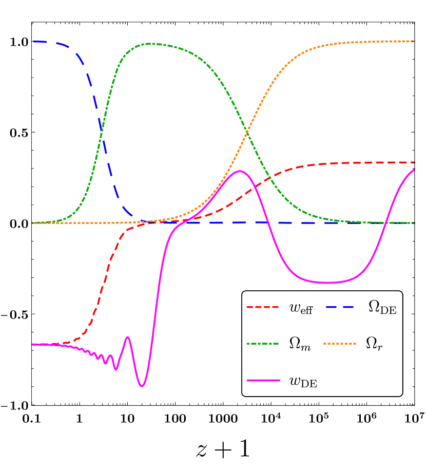
(a)

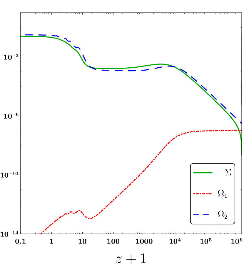
(b)

Figure 1: (a) Evolution of $\Omega_{\rm DE}$, $\Omega_{r}$, $\Omega_{m}$, $w_{\rm DE}$, and $w_{\rm eff}$ versus $z+1$ for $\lambda=\mu=10$, with the initial conditions $X=10^{-13}$, $Y=10^{-14}$, $\Sigma=0$, $\Omega_{1}=10^{-7}$, $\Omega_{2}=10^{-10}$, and $\Omega_{r}=0.99996$ at the redshift $z=7.9\times 10^{7}$. (b) Evolution of $-\Sigma$, $\Omega_{1}$ and $\Omega_{2}$ versus $z+1$ for $\lambda=\mu=10$ with the same set of initial conditions as figure (a).

Instead of the standard analysis of critical points and stability for the previous autonomous system, we decide the make numerical integrations of the equations to obtain a general behavior of the solutions. A complete analysis of this system goes beyond this short paper and is left for a forthcoming work. In fig. 1 we shown the numerical integration of the set of eqs. 22, 23, 24, 25, 26 and 27 where the couplings constants were fixed to be $\lambda=\mu=10$. Typically, we search for a transition from radiation dominance, to matter dominance, and finllay reach an epoch dominated by dark energy today. In terms of effective equation of state $w_{\rm{eff}}$ those transitions are of the type $w_{\rm{eff}}\sim\frac{1}{2}\longrightarrow w_{\rm{eff}}\sim 0\longrightarrow w_{\rm{eff}}\leq-\frac{1}{3}$, as we can see in figure fig. 1a, where the sequence is observed in terms of the density parameters. For large redshifts the radiation dominates and start to decrease at an approximate redshift of $z\sim 3000$ to a matter dominated epoch ($\Omega_{m}\sim 1$), as expected. The evolution of the shear $\Sigma$ and the density parameters $\Omega_{1}$ and $\Omega_{2}$ are shown in fig. 1b. The contribution of the $2-$form always dominate over the $1-$form, except for the initial condition at high redshift ($\sim 10^{7}$); the shear increases until a constant value in the present time. In contrast with the case presented in Ref. 8, where only the $2-$form is considered, $w_{\rm{eff}}$ and $w_{\rm{DE}}$ we will not reach the asymptotic value $\sim-1$. Nevertheless, we check numerically by evolving $w_{\rm{DE}}$ with different (larger) values of the coupling $\mu$, that this value is realized.

As we anticipated, a complete analysis including the stability of fixed points of the autonomous system, will be presented in a future work, where we also want to elucidate the effect of a non-vanishing coupling between the $1-$ and $2-$ form fields.

References

• [1] A. H. Guth and S.-Y. Pi, Fluctuations in the new inflationary universe, Phys. Rev. Lett. 49, 1110 (1982).
• [2] A. Starobinsky, Dynamics of phase transition in the new inflationary universe scenario and generation of perturbations, Phys Lett. B 117, 175 (1982).
• [3] P. A. R. Ade et al., Planck 2015 results. XVI. Isotropy and statistics of the CMB, Astron. Astrophys. 594 A16 (2016).
• [4] M.-a. Watanabe, S. Kanno and J. Soda, Inflationary Universe with Anisotropic Hair, Phys. Rev. Lett. 102, 191302 (2009).
• [5] K. Dimopoulos and M. Karciauskas, Parity Violating Statistical Anisotropy, JHEP 06, 040 (2012).
• [6] J. Ohashi, J. Soda and S. Tsujikawa, Observational signatures of anisotropic inflationary models, JCAP 1312, 009 (2013).
• [7] M. Thorsrud, D. F. Mota and S. Hervik, Cosmology of a Scalar Field Coupled to Matter and an Isotropy-Violating Maxwell Field, JHEP 10, 066 (2012).
• [8] J. P. BeltrΓ‘n Almeida, A. Guarnizo, R. Kase, S. Tsujikawa and C. A. Valenzuela-Toledo, Anisotropic 2-form dark energy, Phys. Lett. B 793, 396 (2019).
• [9] J. P. BeltrΓ‘n Almeida, A. Guarnizo and C. A. Valenzuela-Toledo, Arbitrarily coupled $p-$forms in cosmological backgrounds, [arXiv:1810.05301 [astro-ph.CO]] (2018).
• [10] J. P. BeltrΓ‘n Almeida, A. Guarnizo, R. Kase, S. Tsujikawa and C. A. Valenzuela- Toledo, Anisotropic inflation with coupled $p-$forms, JCAP 1903, 025 (2019).