Viscous Transport in Eroding Porous Media

Abstract

Transport of viscous fluid through porous media is a direct consequence of the pore structure. Here we investigate transport through a specific class of two-dimensional porous geometries, namely those formed by fluid-mechanical erosion. We investigate the tortuosity and dispersion by analyzing the first two statistical moments of tracer trajectories. For most initial configurations, tortuosity decreases in time as a result of erosion increasing the porosity. However, we find that tortuosity can also increase transiently in certain cases. The porosity-tortuosity relationships that result from our simulations are compared with models available in the literature. Asymptotic dispersion rates are also strongly affected by the erosion process, as well as by the number and distribution of the eroding bodies. Finally, we analyze the pore size distribution of an eroding geometry. The simulations are performed by combining a high-fidelity boundary integral equation solver for the fluid equations, a second-order stable time stepping method to simulate erosion, and new numerical methods to stably and accurately resolve nearly-touching eroded bodies and particle trajectories near the eroding bodies.

1 Introduction

Porous media flow plays an important role in many environmental and industrial applications. Depending on the application, length scales can vary from $10^{-6}\mathrm{m}$ to $10^{-1}\mathrm{m}$ (Miller et al., 1998) and velocity scales can be as small as $10^{-1}\mathrm{m/day}$ (Kutsovsky et al., 1996). Moreover, for a single porous geometry, the pore sizes and velocities can range over several orders of magnitude. Numerical methods that resolve this range of scales offer the ability to: (i) characterize dispersion (Saffman, 1959), (ii) quantify mixing (Borgne et al., 2011; Dentz et al., 2011), and (iii) develop meaningful constitutive relationships that link the microscopic and macroscopic realms (Miller et al., 1998). Examples of coarse-grained models for porous media flow include permeability-porosity relationships (Dardis & McCloskey, 1998; Carman, 1937), tortuosities (Matyka et al., 2008; Duda et al., 2011; Koponen et al., 1996), geometry connectivity (Knudby & Carrera, 2005), anomalous dispersion (Dentz et al., 2004), and more.

Flow in porous media is further complicated when boundaries evolve dynamically in response to the fluid flow. This coupling between geometry and flow occurs, for example, in applications involving melting (Beckermann & Viskanta, 1988; Rycroft & Bazant, 2016; Jambon-Puillet et al., 2018; Favier et al., 2019; Morrow et al., 2019), dissolution (Kang et al., 2002; Huang et al., 2015; Moore, 2017; Wykes et al., 2018), deposition (Johnson & Elimelech, 1995; Hewett & Sellier, 2018), biofilm growth (Tang et al., 2015), and crack formation (Cho et al., 2019). We focus on erosion, a fluid-mechanical process that is prevalent in many geophysical, hydrological, and industrial applications (Ristroph et al., 2012; Berhanu et al., 2012; Hewett & Sellier, 2017; Lachaussée et al., 2018; López et al., 2018; Allen, 2019; Amin et al., 2019).

When a porous medium erodes, certain qualitative characteristics are unveiled that affect transport through the geometry. For example, an eroded geometry may contain channels of high porosity, which, though few in number and modest in volume fraction, transmit a large portion of the flux (Quaife & Moore, 2018). This arrangement results in velocities that vary over several orders of magnitude (Alley et al., 2002). Moreover, channelization creates heterogeneous and anisotropic medium properties, which affect the transport of tracers such as contaminants (Cvetkovic et al., 1996; Dagan, 1987; Konikow & Bredehoeft, 1978) and heat (Nilsen & Storesletten, 1990; Rees & Storesletten, 1995).

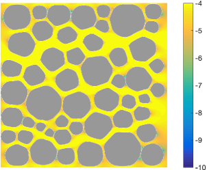
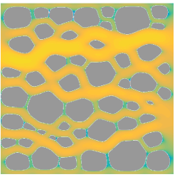
Figure 1: 50 bodies eroding in a Hagen-Poiseuille flow. The six snapshots are equispaced in time, and the color is the magnitude of the fluid velocity in a logarithmic scale. The flow velocity varies over several orders of magnitude, the grains form irregular shapes with large aspect ratios, and the geometry becomes channelized and anisotropic.

This study consists of two main undertakings: first, high-fidelity simulations of eroding porous media, and, second, characterization of tracer transport through the resulting eroded geometries. Our modeling efforts build on previous work (Ristroph et al., 2012; Moore et al., 2013; Moore, 2017), in particular recent numerical methods developed to simulate erosion in the Stokes-flow regime (Quaife & Moore, 2018). We, however, make key improvements to the numerical methods to enable simulations of more realistic, dense suspensions of eroding grains (figures 1 and 2). Then, to characterize transport through these configurations, we examine coarse-grained variables through statistical analysis of tracer trajectories.

Owing to the scales present in groundwater flow (Bear, 1972), we model the hydrodynamics with the two-dimensional incompressible Stokes equations. Meanwhile, individual grains erode at a rate proportional to the hydrodynamic shear stress (Wan & Fell, 2004; Ristroph et al., 2012; Moore et al., 2013; Parker & Izumi, 2000). Since the fluid equations are linear and homogeneous, they are converted to a boundary integral equation (BIE), and this allows us to naturally resolve the non-negligible interactions between bodies. We also compute the vorticity in the fluid bulk since, on solid boundaries, vorticity reduces to shear and thus provides a convenient way to simultaneously visualize local erosion rates and changes in the surrounding flow (figure 2).

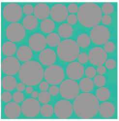
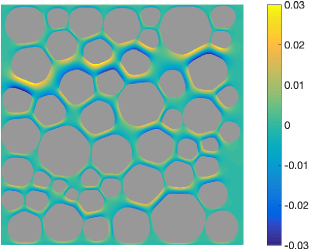
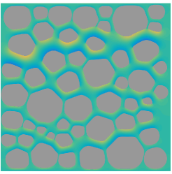
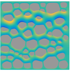
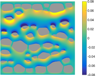
Figure 2: The same six snapshots as figure 1. The color is the vorticity of the fluid. Since the rate of erosion is equivalent to the magnitude of the vorticity, erosion is fastest in the yellow and blue regions and slowest in the green regions.

To compute stable simulations of erosion, we use methods of high-order in both space and time. The time integration is unchanged from previous work (Quaife & Moore, 2018). We apply a mild regularization and a smoothing term to eliminate numerical instabilities that can be triggered by changes in sign of the shear stress, and we use a stable second-order Runge-Kutta method applied to the $\theta$–$L$ coordinates (Hou et al., 1994) of the eroding grains. In this work, we introduce a new quadrature method to resolve dense suspensions. The accuracy of the trapezoid rule, which was used in previous work, is adequate for bodies that are sufficiently separated (Trefethen & Weideman, 2014), but not for grains in close contact. One of the earliest quadrature methods for nearly-singular integrands was developed by Baker & Shelley (1986), and in recent years, many other schemes have followed (af Klinteberg & Tornberg, 2018; Helsing & Ojala, 2008; Beale et al., 2016; Beale & Lai, 2001; Klöckner et al., 2013). We use a Barycentric quadrature method (Barnett, 2014; Barnett et al., 2015) since it is a non-intrusive modification of the trapezoid rule, and the error is guaranteed to be uniformly bounded. We extend the original quadrature method to compute the velocity gradient, which is needed to evaluate the shear stress and the fluid vorticity.

To characterize transport through the resulting configurations, particle trajectories must be computed. Depending on the application, microscale transport can be modelled as pure advection (de Anna et al., 2018; Cvetkovic et al., 1996; Puyguiraud et al., 2019), advection-diffusion (Cushman et al., 1995; Dagan, 1987; Dentz et al., 2018), or with a random walk (Saffman, 1959; Bijeljic & Blunt, 2006; Berkowitz et al., 2000). In this work, we assume trajectories to be governed by pure advection (ie. no diffusion), so the particle trajectories are identical to the streamlines. We compute trajectories ${\mathbf{s}}(t)$ that are initialized at ${\mathbf{s}}_{0}$ by solving the advection equation

$$\frac{d{\mathbf{s}}}{dt}={\mathbf{u}}({\mathbf{s}},t),\quad{\mathbf{s}}(0)={\mathbf{s}}_{0},$$ (1)

where ${\mathbf{u}}$ is the fluid velocity. Since there is no stiff diffusive term, we solve (1) with a fourth-order explicit Runge-Kutta time stepping method. The Barycentric quadrature rule is used to accurately compute trajectories that are close to an eroding grain.

Once the streamlines are computed, we characterize transport by analyzing three different metrics: the tortuosity, the anomalous dispersion, and the pore size distribution. The local tortuosity of a streamline that connects the inlet to the outlet is defined as the streamline’s length normalized by the linear inlet-to-outlet distance. In porous media, the local tortuosity can be greater than 1.5 (Koponen et al., 1996; Matyka et al., 2008) or even 2 (Duda et al., 2011), depending on several factors such as the porosity. The tortuosity of a geometry is defined by averaging the local tortuosity over all streamlines initialized at the inlet, and the geometry’s tortuosity characterizes average particle motions (Hakoun et al., 2019). To characterize spreading, the fluid dispersion is defined as the variance of the streamline lengths. In porous media, this spreading is often super-dispersive (Kang et al., 2014; Cushman et al., 1995; de Anna et al., 2013). Since anomalous dispersion results from streamlines spending time in both the high and low velocity regimes (Berkowitz & Scher, 2001), it is crucial to accurately resolve streamlines near grain boundaries, as achieved in this work. Finally, we construct the pore-size distribution throughout the erosion process. These distributions are required to quantify velocity distributions (Alim et al., 2017; de Anna et al., 2018), channelization (Siena et al., 2019), connectivity (Knudby & Carrera, 2005; Western et al., 2001), and to develop network models (Bryant et al., 1993a, b; Bijeljic & Blunt, 2006).

This paper is organized as follows. In section 2, we summarize the erosion model that is described in more detail in previous work (Quaife & Moore, 2018). In section 3, we recast all the governing equations as layer potentials defined in both ${\mathbb{R}}^{2}$ and in ${\mathbb{C}}$. Section 4 describes measures for characterizing the geometry and transport. Section 5 describes the numerical methods, with special attention paid to the new quadrature method for computing the shear stress and the vorticity. Section 6 presents numerical examples for a variety of dense packings of bodies. Finally, concluding remarks are made in section 7.

2 Governing Equations

We start by defining the main variables used to model erosion. We only briefly summarize the model, and a more detailed description can be found in previous work (Quaife & Moore, 2018). We consider flows inside a confined geometry $\Omega$ that contains $M$ eroding bodies with boundaries $\gamma_{\ell}$, $\ell=1,\ldots,M$. The boundary of the fluid domain is ${\partial}\Omega=\Gamma\cup\gamma_{1}\cup\cdots\cup\gamma_{M}$, where $\Gamma$ is the outer boundary, taken to be a slightly smoothed version of the boundary of $[-3,3]\times[-1,1]$. All eroding bodies are placed in $[-1,1]\times[-1,1]$ to create a buffer region that allows the flow profile imposed at the inlet to transition to the more complex flow intervening between the bodies. Neglecting inertial forces, the governing equations are

$$\begin{split}\mu\Delta{\mathbf{u}}={\nabla}p,&\hskip 20.0pt{\mathbf{x}}\in\Omega,\hskip 14.45377pt&&\mbox{\em conservation of momentum},\\ {\nabla}\cdot{\mathbf{u}}=0,&\hskip 20.0pt{\mathbf{x}}\in\Omega,\hskip 14.45377pt&&\mbox{\em conservation of mass},\\ {\mathbf{u}}=\mathbf{0},&\hskip 20.0pt{\mathbf{x}}\in\gamma,\hskip 14.45377pt&&\mbox{\em no slip on the eroding bodies},\\ {\mathbf{u}}={\mathbf{U}},&\hskip 20.0pt{\mathbf{x}}\in\Gamma,\hskip 14.45377pt&&\mbox{\em outer wall velocity},\\ V_{\mathbf{n}}=C_{E}\,\lvert\tau\rvert,&\hskip 20.0pt{\mathbf{x}}\in\gamma,&&\mbox{\em erosion model}.\end{split}$$ (2)

Here ${\mathbf{u}}$ is the fluid velocity, $p$ is the pressure, ${\mathbf{U}}$ is a prescribed Hagen-Poiseuille velocity field, and $V_{\mathbf{n}}$ is the normal velocity of $\gamma$. The shear stress on $\gamma$ is

$$\tau=-(\nabla{\mathbf{u}}+\nabla{\mathbf{u}}^{T}){\mathbf{n}}\cdot{\mathbf{s}}$$ (3)

where, ${\mathbf{n}}$ is the normal vector pointing into the body, and ${\mathbf{s}}$ is the unit tangent vector pointing in the counterclockwise direction. We simulate erosion by alternating between solving the fluid equations and advancing the eroding grains. The strength of ${\mathbf{U}}$ is adjusted at each time step to achieve a constant pressure drop across the channel, motivated by the geological situation of a porous medium connecting two regions of fixed hydraulic heads.

3 Boundary Integral Equation Formulation

To accurately solve the governing equations (2) in complex two-dimensional geometries, we reformulate the equations as a BIE. This has the advantage that only the one-dimensional boundary of the domain must be discretized, and, with appropriate quadrature formulas and fast summation methods, the result is a high-fidelity numerical simulation with near-optimal computational complexity.

3.1 Double-Layer Potential Formulation in ${\mathbb{R}}^{2}$

Applying the same approach as our previous work (Quaife & Moore, 2018), we start with the double-layer potential

$${\boldsymbol{\mathcal{D}}}[{\boldsymbol{\eta}}]({\mathbf{x}})=\int_{{\partial}\Omega}D({\mathbf{x}},{\mathbf{y}}){\boldsymbol{\eta}}({\mathbf{y}})\,ds_{\mathbf{y}}=\frac{1}{\upi}\int_{{\partial}\Omega}\frac{{\mathbf{r}}\cdot{\mathbf{n}}}{\rho^{2}}\frac{{\mathbf{r}}\otimes{\mathbf{r}}}{\rho^{2}}{\boldsymbol{\eta}}({\mathbf{y}})\,ds_{\mathbf{y}},\quad{\mathbf{x}}\in\Omega,$$ (4)

where $D$ is the kernel of the integral operator, ${\mathbf{r}}={\mathbf{x}}-{\mathbf{y}}$, $\rho=\|{\mathbf{r}}\|$, ${\mathbf{n}}$ is the unit outward normal at ${\mathbf{y}}$, and ${\boldsymbol{\eta}}$ is an unknown density function. We complete the integral equation formulation by adding the $M$ Stokeslets, $S[{\boldsymbol{\lambda}}_{\ell},{\mathbf{c}}_{\ell}]({\mathbf{x}})$, and $M$ rotlets, $R[\xi_{\ell},{\mathbf{c}}_{\ell}]({\mathbf{x}})$, where ${\mathbf{c}}_{\ell}$ is a point inside the $\ell^{th}$ body (Power & Miranda, 1987). Here ${\boldsymbol{\lambda}}_{\ell}$ and $\xi_{\ell}$ are the Stokeslet and rotlet strengths, respectively, corresponding to the $\ell^{th}$ body. Then, for any sufficiently smooth geometry $\Omega$, the solution of the incompressible Stokes equation with a Dirichlet boundary condition ${\mathbf{f}}$ is

$${\mathbf{u}}({\mathbf{x}})={\boldsymbol{\mathcal{D}}}[{\boldsymbol{\eta}}]({\mathbf{x}})+\sum_{\ell=1}^{M}S[{\boldsymbol{\lambda}}_{\ell},{\mathbf{c}}_{\ell}]({\mathbf{x}})+\sum_{\ell=1}^{M}R[\xi_{\ell},{\mathbf{c}}_{\ell}]({\mathbf{x}}),\quad{\mathbf{x}}\in\Omega,$$ (5)

where the density function, Stokeslets, and rotlets satisfy

$${\mathbf{f}}({\mathbf{x}}) =-\frac{1}{2}{\boldsymbol{\eta}}({\mathbf{x}})+{\boldsymbol{\mathcal{D}}}[{\boldsymbol{\eta}}]({\mathbf{x}})+{\mathcal{N}}_{0}[{\boldsymbol{\eta}}]({\mathbf{x}})$$

$$\quad+\sum_{\ell=1}^{M}S[{\boldsymbol{\lambda}}_{\ell},{\mathbf{c}}_{\ell}]({\mathbf{x}})+\sum_{\ell=1}^{M}R[\xi_{\ell},{\mathbf{c}}_{\ell}]({\mathbf{x}}),\quad \qquad{\mathbf{x}}\in{\partial}\Omega,$$ (6a)

$${\boldsymbol{\lambda}}_{\ell} =\frac{1}{2\upi}\int_{\gamma_{\ell}}{\boldsymbol{\eta}}({\mathbf{y}})\,ds_{\mathbf{y}}, \qquad\ell=1,\ldots,M,$$ (6b)

$$\xi_{\ell} =\frac{1}{2\upi}\int_{\gamma_{\ell}}({\mathbf{y}}-{\mathbf{c}}_{\ell})^{\perp}\cdot{\boldsymbol{\eta}}({\mathbf{y}})\,ds_{\mathbf{y}}, \qquad\ell=1,\ldots,M.$$ (6c)

Here, the null space associated with the flux-free condition of ${\mathbf{f}}$ is addressed with ${\mathcal{N}}_{0}$ which is the integral operator with kernel $N_{0}({\mathbf{x}},{\mathbf{y}})={\mathbf{n}}({\mathbf{x}})\otimes{\mathbf{n}}({\mathbf{y}})$, ${\mathbf{x}},{\mathbf{y}}\in\Gamma$. In this work, ${\mathbf{f}}$ is the prescribed velocity, which is equal to ${\mathbf{U}}$ on the outer wall, $\Gamma$, and equal to zero on the eroding bodies, $\gamma_{\ell}$, $\ell=1,\ldots,M$.

Once (6) is solved for the density function ${\boldsymbol{\eta}}$, the corresponding deformation tensor, pressure, and vorticity at ${\mathbf{x}}\in\Omega$ are written in terms of layer potentials (Quaife & Moore, 2018). To compute the deformation tensor for ${\mathbf{x}}\in\gamma$, we include the jump term

$$\frac{1}{2}\left(\frac{\partial{\boldsymbol{\eta}}}{\partial{\mathbf{s}}}\cdot{\mathbf{s}}\right)\left[\begin{array}[]{cc}s_{x}^{2}-s_{y}^{2}&2s_{x}s_{y}\\ 2s_{x}s_{y}&s_{y}^{2}-s_{x}^{2}\end{array}\right].$$ (9)

Finally, the deformation tensor, pressure, and vorticity due to the Stokeslets and rotlets are readily available (Pozrikidis, 1992). Having computed the deformation tensor on $\gamma$, the shear stress is computed using equation (3).

3.2 Cauchy Integral Representation of the Double-Layer Potential

The velocity double-layer potential (4), and its corresponding deformation tensor, pressure, and vorticity are all written as layer potentials in ${\mathbb{R}}^{2}$. However, the quadrature method we introduce in section 5 requires complex-valued representations. The first step to form a complex representation is to write the Laplace double-layer potential as the complex integral

$${\mathcal{D}}[{\boldsymbol{\eta}}]({\mathbf{x}})=\frac{1}{2\upi}\int_{{\partial}\Omega}\frac{{\mathbf{r}}\cdot{\mathbf{n}}}{\rho^{2}}{\boldsymbol{\eta}}({\mathbf{y}})\,ds_{\mathbf{y}}=\Real(v(x)),$$ (10)

where

$$v(x)=\frac{1}{2\upi i}\int_{{\partial}\Omega}\frac{\eta(y)}{x-y}\,dy,\quad x\in\Omega.$$ (11)

Here $x=x_{1}+ix_{2},y=y_{1}+iy_{2}\in{\mathbb{C}}$ are the complex counterparts of ${\mathbf{x}}=(x_{1},x_{2}),{\mathbf{y}}=(y_{1},y_{2})\in{\mathbb{R}}^{2}$, and $\eta=\eta_{1}+i\eta_{2}$ is the complex counterpart of ${\boldsymbol{\eta}}=(\eta_{1},\eta_{2})$. Therefore, depending on the formulation of the layer potential, $\Omega$ is interpreted as a subset of ${\mathbb{R}}^{2}$ or ${\mathbb{C}}$. Equation (11) is converted to a Cauchy integral by first finding the boundary data of $v$. If $\Omega$ is a simply-connected interior domain, then the boundary data of $v$ satisfies the Sokhotski-Plemelj jump relation

$$v(x)=-\frac{1}{2}\eta(x)+\frac{1}{2\upi i}\int_{{\partial}\Omega}\frac{\eta(y)}{x-y}\,dy,\quad x\in{\partial}\Omega.$$ (12)

For exterior domains, the jump term changes from $-1/2$ to $1/2$, and for multiply-connected domains, such as a porous media, ${\partial}\Omega$ is decomposed into its different connected components and the appropriate jump relation is applied. Having computed the boundary data of the holomorphic function $v$, by the Cauchy integral theorem we have

$$v(x) =\frac{1}{2\upi i}\int_{{\partial}\Omega}\frac{v(y)}{y-x}\,dy,$$ (13a)

$$v^{\prime}(x) =\frac{1}{2\upi i}\int_{{\partial}\Omega}\frac{v(y)}{(y-x)^{2}}\,dy,$$ (13b)

$$v^{\prime\prime}(x) =\frac{1}{\upi i}\int_{{\partial}\Omega}\frac{v(y)}{(y-x)^{3}}\,dy,$$ (13c)

for $x\in\Omega$. Since $v(x)$ depends on the complex-valued density function $\eta$, we use the notation $v[\eta](x)$ for the holomorphic function defined in equation (11), and its first two derivatives are written as $v^{\prime}[\eta](x)$ and $v^{\prime\prime}[\eta](x)$.

Finally, the Stokes double-layer potential (4) can be written using a Laplace double-layer potential (11) and its gradients

$${\boldsymbol{\mathcal{D}}}[{\boldsymbol{\eta}}]({\mathbf{x}}) =\frac{1}{2\upi}\int_{{\partial}\Omega}\frac{{\mathbf{n}}}{\rho^{2}}({\mathbf{r}}\cdot{\boldsymbol{\eta}})\,ds_{\mathbf{y}}+\frac{1}{2\upi}\nabla\int_{{\partial}\Omega}\frac{{\mathbf{r}}\cdot{\mathbf{n}}}{\rho^{2}}({\mathbf{y}}\cdot{\boldsymbol{\eta}})\,ds_{\mathbf{y}}$$ (14)

$$-\frac{1}{2\upi}x_{1}\nabla\int_{{\partial}\Omega}\frac{{\mathbf{r}}\cdot{\mathbf{n}}}{\rho^{2}}\eta_{1}({\mathbf{y}})\,ds_{\mathbf{y}}-\frac{1}{2\upi}x_{2}\nabla\int_{{\partial}\Omega}\frac{{\mathbf{r}}\cdot{\mathbf{n}}}{\rho^{2}}\eta_{2}({\mathbf{y}})\,ds_{\mathbf{y}}.$$

Therefore, the Stokes double-layer potential can be written as a sum of Cauchy integrals and its first derivative (Barnett et al., 2015)

$$u_{1}(x) =\Real(v[\psi_{1}](x))+\Real(v^{\prime}[y\cdot\eta](x))-x_{1}\Real(v^{\prime}[\eta_{1}](x))-x_{2}\Real(v^{\prime}[\eta_{2}](x)),$$ (15)

$$u_{2}(x) =\Real(v[\psi_{2}](x))-\Imag(v^{\prime}[y\cdot\eta](x))+x_{1}\Imag(v^{\prime}[\eta_{1}](x))+x_{2}\Imag(v^{\prime}[\eta_{2}](x)),$$

where $y\cdot\eta=y_{1}\eta_{1}+y_{2}\eta_{2}$,

$$\psi_{1}=(\eta_{1}+i\eta_{2})\frac{\Real(n)}{n},\quad\psi_{2}=(\eta_{1}+i\eta_{2})\frac{\Imag(n)}{n},$$ (16)

and $n\in{\mathbb{C}}$ is the complex counterpart of the outward unit normal ${\mathbf{n}}\in{\mathbb{R}}^{2}$.

3.3 Cauchy Integral Representation for the Gradient of the Double-Layer Potential

Computing the shear stress and vorticity requires a complex-valued layer potential representation of the velocity gradient. The deformation tensor at $x\in\Omega$ is found by computing the derivatives of the expressions for $u_{1}$ and $u_{2}$ in equation (15)

$$\frac{\partial u_{1}}{\partial x_{1}} =+\Real(v^{\prime}[\psi_{1}](x))+\Real(v^{\prime\prime}[y\cdot\eta](x))-\Real(v^{\prime}[\eta_{1}](x))$$ (17)

$$-x_{1}\Real(v^{\prime\prime}[\eta_{1}](x))-x_{2}\Real(v^{\prime\prime}[\eta_{2}](x)),$$

$$\frac{\partial u_{1}}{\partial x_{2}} =-\Imag(v^{\prime}[\psi_{1}](x))-\Imag(v^{\prime\prime}[y\cdot\eta](x))+x_{1}\Imag(v^{\prime\prime}[\eta_{1}](x))$$

$$-\Real(v^{\prime}[\eta_{2}](x))+x_{2}\Imag(v^{\prime\prime}[\eta_{2}](x)),$$

$$\frac{\partial u_{2}}{\partial x_{1}} =+\Real(v^{\prime}[\psi_{2}](x))-\Imag(v^{\prime\prime}[y\cdot\eta](x))+\Imag(v^{\prime}[\eta_{1}](x))$$

$$+x_{1}\Imag(v^{\prime\prime}[\eta_{1}](x))+x_{2}\Imag(v^{\prime\prime}[\eta_{2}](x)),$$

$$\frac{\partial u_{2}}{\partial x_{2}} =-\Imag(v^{\prime}[\psi_{2}](x))-\Real(v^{\prime\prime}[y\cdot\eta](x))+x_{1}\Real(v^{\prime\prime}[\eta_{1}](x))$$

$$+\Imag(v^{\prime}[\eta_{2}](x))+x_{2}\Real(v^{\prime\prime}[\eta_{2}](x)).$$

The same expressions are used to compute the deformation tensor for $x\in{\partial}\Omega$, except that the jump condition (9) is included. Finally, to compute the shear stress, the deformation tensor on ${\partial}\Omega$ is applied to the normal and tangent vectors as in equation (3). The velocity gradient is also used to compute the vorticity in the fluid bulk. For $x\in\Omega$, the Cauchy integral representation of the vorticity at $x\in\Omega$ is

$$\omega(x)=\Real(v^{\prime}[\psi_{2}](x))+\Imag(v^{\prime}[\psi_{1}](x))+\Real(v^{\prime}[\eta_{2}](x))+\Imag(v^{\prime}[\eta_{1}](x)).$$ (18)

4 Transport, Tracers, and Tortuosity

Erosion in porous media leads to phenomena such as channelization (Berhanu et al., 2012), and we are interested in characterizing transport in such geometries. In our previous work (Quaife & Moore, 2018), we examined the effect of erosion on the area fraction, flow rate, and the total drag. However, to characterize macroscopic signatures of the transport, other quantities must be examined. Here, we compute the anomalous dispersion rate, the tortuosity, and the distribution of the pore sizes. The first two metrics are defined in terms of streamlines governed by the autonomous advection equation (1).

4.1 Anomalous Dispersion

The spreading of fluid in a porous media is often characterized in terms of anomalous dispersion (Klages et al., 2008; Dentz et al., 2004). The anomalous dispersion rate depends on the porosity and permeability (Koch & Brady, 1988), but is also affected by the distribution and shape of the grains. We calculate the anomalous dispersion rates by analyzing the streamlines governed by equation (1) in eroded geometries. Given a set of $N_{p}$ trajectories, we define $\lambda_{j}(t)$ to be the arclength of the trajectory

$$\lambda_{j}(t)=\int_{0}^{t}\|{\mathbf{s}}^{\prime}_{j}(\tilde{t})\|\,d\tilde{t},\quad j=1,\ldots,N_{p}.$$ (19)

Then, the first and second ensemble moments are

$$\langle\lambda\rangle(t)=\frac{1}{N_{p}}\sum_{j=1}^{N_{p}}\lambda_{j}(t),\quad\sigma_{\lambda}^{2}(t)=\frac{1}{N_{p}}\sum_{j=1}^{N_{p}}\left[\lambda_{j}(t)-\langle\lambda\rangle(t)\right]^{2},$$ (20)

and $\sigma_{\lambda}$ characterizes the dispersion. At early times, the particles have not explored much of the geometry, and we expect a ballistic motion $\sigma_{\lambda}\sim t$. However, as the particles pass the grains, their trajectories are altered, and we expect that $\sigma_{\lambda}\sim t^{\alpha}$, with $\alpha\in(0.5,1)$, indicating that the flow is super-dispersive.

To establish an asymptotic anomalous dispersion rate, the trajectories must pass several grains. The geometries that we consider are too short to observe asymptotic dispersion, so we use a reinsertion method to form longer trajectories. Similar to the work of others (de Anna et al., 2018; Puyguiraud et al., 2019), once a particle reaches the outlet of the porous region, it is reinserted at the inlet. To minimize errors caused by reinsertion, the particle is initialized at the discretization point that has the closest velocity to the particle’s velocity at the outlet. After a single trajectory is formed, it has undergone a collection of reinsertions. Then, as a post-processing step, the trajectory is made continuous by attaching the tail of each segment to the origin of the next segment.

4.2 Tortuosity

The tortuosity is a dimensionless number that quantifies the amount of twisting of streamlines. Unlike the dispersion calculations, we do not use reinsertion to form long trajectories. The local tortuosity is

$$\tau(y_{0})=\frac{\lambda(y_{0})}{d}.$$ (21)

Here the streamline originates on the inlet cross-section $x=x_{0}$ at $(x_{0},y_{0})$, and its arclength, $\lambda(y_{0})$, is calculated until the streamline passes the parallel outlet cross-section $x=x_{0}+d$. In this work, we consider streamlines originating at $x=-1$ and terminating at $x=1$, so $d=2$. However, other choices for the terminal point when computing the tortuosity are sometime used (Duda et al., 2011). The hydraulic tortuosity is defined by taking the average over all points on the inlet cross-section

$$T=\frac{1}{d}\left(\int_{S}u_{1}(x_{0},y_{0})\lambda(y_{0})\,dy_{0}\right)\Bigg{/}\left(\int_{S}u_{1}(x_{0},y_{0})\,dy_{0}\right),$$ (22)

where $S$ is the inlet cross-section $x=-1$, $u_{1}(y_{0})$ is the $x$-component of the velocity at the initial point of the streamline, and $d=2$ is the distance between the inlet and outlet. Note that $T\geq 1$, and $T=1$ only if no grains are present.

The tortuosity can also be computed with an area integral. Assuming that the flow is incompressible and not re-entrant, meaning that all streamlines connect the two cross-sections, the tortuosity in equation (22) is equivalent to (Duda et al., 2011)

$$T=\left(\int_{\Omega}\|{\mathbf{u}}({\mathbf{y}})\|\,d{\mathbf{y}}\right)\Bigg{/}\left(\int_{\Omega}u_{1}({\mathbf{y}})\,d{\mathbf{y}}\right),$$ (23)

where $\Omega$ is the fluid region between the inlet and outlet cross-sections. Recirculation zones are possible in viscous fluids (Higdon, 1985), but they are very small in the examples we consider and have a negligible effect on the tortuosity. Since equation (23) does not require the additional work of computing particle trajectories at every time step, we use this definition for the majority of the tortuosity calculations. However, we do compare the two definitions for the tortuosity at several porosities in section 6.

There have been efforts to relate the tortuosity, $T$, to the porosity, $\phi$. For example, Matyka et al. (2008) propose the models

$$\widehat{T}(\phi) =\phi^{-p},$$ (24a)

$$\widehat{T}(\phi) =1-p\log\phi,$$ (24b)

$$\widehat{T}(\phi) =1+p(1-\phi),$$ (24c)

$$\widehat{T}(\phi) =(1+p(1-\phi))^{2},$$ (24d)

where $p>0$ is a fitting parameter. In section 6, we compare these four models with the tortuosity of eroding porous geometries.

4.3 Pore Throat Size

(a)

(b)

Figure 3: (a) The pore sizes between neighboring grains. Two grains are neighbors if they share an edge of the Delanuay triangulation with nodes at the center of each eroding grain. (b) The pore sizes of an eroded geometry. The black curve is the Weibull distribution with the same first two moments as the data.

While transport in porous media depends on the porosity, it also depends on the placement of the grains. In particular, grain placement affects velocity scales (Alim et al., 2017), correlation structures (Borgne et al., 2007), contaminant transport (Knudby & Carrera, 2005), channelization (Siena et al., 2019; Berhanu et al., 2012), and pore network models (Bryant et al., 1993a, b; Bijeljic & Blunt, 2006). To characterize the grain placement, we compute distributions of pore sizes between neighboring grains. To define neighboring grains, we form the Delaunay triangulation using nodes placed at the center of each eroding grain and at a collection of points around the boundary of the porous media. Then, we say that two grains are neighbors if their centers share an edge of the triangulation (de Anna et al., 2018). The pores of an eroded geometry are illustrated in figure 3(a). We do not consider pores between eroding bodies and the solid wall $\Gamma$, so some of the grains near the porous region boundary only have two neighbors. Having defined the pore sizes, we plot its distribution in figure 3(b) and compare it with the Weibull distribution, a distribution used by others to characterize pore sizes (Ioannidis & Chatzis, 1993). In section 6.4, we investigate the effect of erosion on the pore size distribution.

5 Numerical Methods

In line with our previous work (Quaife & Moore, 2018), we use two meshes to simulate erosion. The integral equation is solved by discretizing the boundary of the geometry at a set of collocation points distributed equally in arclength (section 5.1). Depending on the proximity of the target point to the source points, the quadrature rule is either the trapezoid rule or the Barycentric quadrature rule (section 5.2). The criteria that determines which quadrature method is applied is described in section 5.3. Once the shear stress is computed, the bodies are eroded a single time step by using a $\theta$–$L$ discretization (Hou et al., 1994; Moore et al., 2013). The time stepping methods for erosion and passive particles are described in section 5.4.

5.1 Spatial Discretization

Since we use a BIE formulation, we only need to discretize the one-dimensional boundary of the domain. We discretize each eroding grain $\gamma_{k}$ with $N_{\mathrm{in}}$ points and discretize the outer wall $\Gamma$ with $N_{\mathrm{out}}$ points. The $j^{th}$ discretization point on $\Gamma$ and $\gamma_{k}$ are denoted by ${\mathbf{y}}_{j}^{0}$ and ${\mathbf{y}}^{k}_{j}$, respectively. The discretization points are initially distributed evenly in arclength, and this equispacing is maintained throughout the entire simulation by using the $\theta$–$L$ formulation. In addition, we apply regularization (Quaife & Moore, 2018) to slightly smooth the corners that inevitably develop during erosion.

Given the discretization points of ${\partial}\Omega$, the trapezoid rule results in the collocation method for (6)

$${\mathbf{U}}_{\ell} =\sum_{j=1}^{N_{\mathrm{out}}}w^{0}_{j}D({\mathbf{y}}^{0}_{\ell},{\mathbf{y}}^{0}_{j}){\boldsymbol{\eta}}_{j}^{0}+\sum_{k=1}^{M}\sum_{j=1}^{N_{\mathrm{in}}}w^{k}_{j}D({\mathbf{y}}^{0}_{\ell},{\mathbf{y}}^{k}_{j}){\boldsymbol{\eta}}^{k}_{j}+\sum_{j=1}^{N_{\mathrm{out}}}w^{0}_{j}N_{0}({\mathbf{y}}^{0}_{\ell},{\mathbf{y}}^{0}_{j}){\boldsymbol{\eta}}_{j}^{0}$$

$$+\sum_{k=1}^{M}S[{\boldsymbol{\lambda}}_{k},{\mathbf{c}}_{k}]({\mathbf{y}}^{0}_{\ell})+\sum_{k=1}^{M}R[\xi_{k},{\mathbf{c}}_{k}]({\mathbf{y}}^{0}_{\ell}), \ell=1,\ldots,N_{\mathrm{out}},$$ (25a)

$$\mathbf{0} =\sum_{j=1}^{N_{\mathrm{out}}}w^{0}_{j}D({\mathbf{y}}^{m}_{\ell},{\mathbf{y}}^{0}_{j}){\boldsymbol{\eta}}_{j}^{0}+\sum_{k=1}^{M}\sum_{j=1}^{N_{\mathrm{in}}}w^{k}_{j}D({\mathbf{y}}^{m}_{\ell},{\mathbf{y}}^{k}_{j}){\boldsymbol{\eta}}^{k}_{j}$$

$$+\sum_{k=1}^{M}S[{\boldsymbol{\lambda}}_{k},{\mathbf{c}}_{k}]({\mathbf{y}}^{m}_{\ell})+\sum_{k=1}^{M}R[\xi_{k},{\mathbf{c}}_{k}]({\mathbf{y}}^{m}_{\ell}), m=1,\ldots,M,\>\ell=1,\ldots,N_{\mathrm{in}},$$ (25b)

$${\boldsymbol{\lambda}}_{m} =\frac{1}{2\upi}\sum_{j=1}^{N_{\mathrm{in}}}w_{j}^{m}{\boldsymbol{\eta}}^{m}_{j}, m=1,\ldots,M$$ (25c)

$$\xi_{m} =\frac{1}{2\upi}\sum_{j=1}^{N_{\mathrm{in}}}w_{j}^{m}({\mathbf{y}}^{m}_{j}-{\mathbf{c}}_{m})^{\perp}\cdot{\boldsymbol{\eta}}^{m}_{j}, m=1,\ldots,M,$$ (25d)

where $w^{k}_{j}$ are quadrature weights that depend on $N_{\mathrm{in}}$, $N_{\mathrm{out}}$, and the lengths of $\gamma^{k}$ and $\Gamma$, and $D$ is the kernel of the Stokes double-layer potential defined in equation (4). Since the kernel is smooth, the diagonal terms $D({\mathbf{y}}_{j}^{m},{\mathbf{y}}_{j}^{m})$ are replaced with the appropriate curvature-dependent limiting term. The linear system (25) is a well-conditioned second-kind integral equation and is solved iteratively with GMRES. If the number of discretization points is sufficiently large, then the solution of (25) is an accurate approximation of the density function, Stokeslets, and rotlets. Then, for ${\mathbf{x}}\in\Omega$, the double-layer potential is approximated as

$${\mathbf{u}}({\mathbf{x}}) =\sum_{j=1}^{N_{\mathrm{out}}}w^{0}_{j}D({\mathbf{x}},{\mathbf{y}}^{0}_{j}){\boldsymbol{\eta}}_{j}+\sum_{k=1}^{M}\sum_{j=1}^{N_{\mathrm{in}}}w^{k}_{j}D({\mathbf{x}},{\mathbf{y}}^{k}_{j}){\boldsymbol{\eta}}^{k}_{j}.$$ (26)

Similarly, the corresponding layer potentials for the deformation tensor and vorticity are approximated with the trapezoid rule. The contributions due to the Stokeslets and rotlets require no quadrature and are easily included in the velocity, deformation tensor, and vorticity. Finally, Fourier differentiation is used to compute the jump term (9) of the shear stress, and then the tensor is applied to the normal and tangent vectors as defined in equation (3).

Once the velocity is computed in $\Omega$, the tortuosity can be computed with the Eulerian velocity field (23). We compute the velocity at ${\mathbf{x}}_{ij}=(-1+i\Delta x,-1+j\Delta y)$, $i,j=1,\ldots,N$, where $\Delta x=\Delta y=2/N$, and the velocity at points inside an eroding body are assigned a value of 0. Then, the tortuosity is approximated as

$$T=\left(\sum_{i,j=1}^{N}\|{\mathbf{u}}({\mathbf{x}}_{ij})\|\Delta x\Delta y\right)\Bigg{/}\left(\sum_{i,j=1}^{N}u_{1}({\mathbf{x}}_{ij})\Delta x\Delta y\right)$$ (27)

5.2 Barycentric Quadrature Formulas

While the trapezoid rule is spectrally accurate for smooth, periodic functions (Trefethen & Weideman, 2014), the derivative of the integrand grows as the target point ${\mathbf{x}}$ approaches ${\partial}\Omega$. Therefore, if the trapezoid rule is applied when bodies are in near-contact, or if a layer potential is evaluated at a point close to ${\partial}\Omega$, then the result become unreliable and the simulation ultimately becomes unstable. We thus desire a quadrature method whose error bound does not depend on the target location.

We showed in sections 3.2 and 3.3 that the velocity, shear stress, and vorticity of the double-layer representation can all be written as the sum of Cauchy integrals and its first two derivatives. Therefore, we require quadrature rules with a uniform error bound for Cauchy integrals and its derivatives (13). Ioakimidis et al. (1991) developed quadrature rules, that we call Barycentric quadrature rules, to compute Cauchy integrals and their derivatives with an error bound that is independent of $x\in{\mathbb{C}}$. Then, Barnett et al. (2015) used these quadrature rules to compute the Stokes double-layer potential representation of the velocity (4). After briefly summarizing this method, we extend the work to compute the second derivative so that the shear stress and vorticity can be computed with a uniform error bound.

We present the quadrature rules for a simply-connected interior domain $\Omega\subset{\mathbb{C}}$, with any point $a\in\Omega$, and we consider target points $x\in\Omega$ and $x\in\Omega^{c}$. Then, the quadrature rules can be applied to individual components of a multiply-connected domain to compute the velocity, vorticity, and deformation tensor in an eroding porous media. The method starts with an underlying quadrature rule, and we use the spectrally accurate $N$-point trapezoid rule. Since the quadrature points are uniformly distributed, the quadrature weights are $w_{j}=L/N$, $j=1,\ldots,N$, where $L$ is the length of ${\partial}\Omega$.

Again, given a complex-valued density function $\eta$, the boundary data of $v[\eta](x)$, as defined in equation (11), satisfies the Sokhotski-Plemelj jump relation (12). Since the limiting boundary data of $v$ differs when considering $x\in\Omega$ and $x\in\Omega^{c}$, we denote the boundary data as $v^{-}$ for $x\in\Omega$, and as $v^{+}$ for $x\in\Omega^{c}$. Rather than directly applying the trapezoid rule to approximate $v(x)$ in equation (13), we start with the identity

$$\int_{{\partial}\Omega}\frac{v^{-}(y)-v(x)}{y-x}\,dy=0,\quad x\in\Omega.$$ (28)

Since the integrand is bounded for all $x\in\Omega$, we can apply the trapezoid rule

$$\sum_{j=1}^{N}\frac{v^{-}(y_{j})-v(x)}{y_{j}-x}w_{j}\approx 0,$$ (29)

and the error is independent of $x$. Rearranging for $v(x)$, we have the interior Barycentric quadrature rule

$$v(x)=\left(\sum_{j=1}^{N}\frac{v^{-}(y_{j})}{y_{j}-x}w_{j}\right)\Bigg{/}\left(\sum_{j=1}^{N}\frac{1}{y_{j}-x}w_{j}\right),\quad x\in\Omega.$$ (30)

Using a similar construction and letting $a$ be any point inside $\Omega$, the exterior Barycentric quadrature rule is

$$v(x)=\frac{1}{x-a}\left(\sum_{j=1}^{N}\frac{v^{+}(y_{j})}{y_{j}-x}w_{j}\right)\Bigg{/}\left(\sum_{j=1}^{N}\frac{(y_{j}-a)^{-1}}{y_{j}-x}w_{j}\right),\quad x\in\Omega^{c}.$$ (31)

Similar constructions can be used to derive quadrature rules for $v^{\prime}(x)$. For $x\in\Omega$, we have the identity

$$\int_{{\partial}\Omega}\frac{v^{-}(y)-v(x)+(y-x)v^{\prime}(x)}{(y-x)^{2}}=0,$$ (32)

and the integrand is bounded for all $x\in\Omega$. Therefore, after applying the trapezoid rule and rearranging for $v^{\prime}(x)$, we have the interior Barycentric quadrature rule

$$v^{\prime}(x)=\left(\sum_{j=1}^{N}\frac{v^{-}(y_{j})-v(x)}{(y_{j}-x)^{2}}w_{j}\right)\Bigg{/}\left(\sum_{j=1}^{N}\frac{1}{y_{j}-x}w_{j}\right),\quad x\in\Omega.$$ (33)

Using a similar construction, the exterior Barycentric quadrature rule for the first derivative is

$$v^{\prime}(x)=\frac{1}{x-a}\left(\sum_{j=1}^{N}\frac{v^{+}_{j}-v(x)}{(y_{j}-x)^{2}}w_{j}\right)\Bigg{/}\left(\sum_{j=1}^{N}\frac{(y_{j}-a)^{-1}}{y_{j}-x}w_{j}\right),\quad x\in\Omega^{c}.$$ (34)

Note that $v(x)$ is required to compute $v^{\prime}(x)$ for both the interior and exterior case, and this is available using the Barycentric quadrature rules (30) and (31).

To compute the shear stress and vorticity, we require a Barycentric quadrature rule for $v^{\prime\prime}(x)$. The derivation is largely based on the work of Ioakimidis et al. (1991, see equation (2.12)). We start with the second derivative of the Cauchy integral theorem

$$0=\frac{1}{2\upi i}\int_{{\partial}\Omega}\frac{2v^{-}(y)}{(y-x)^{3}}\,dy-v^{\prime\prime}(x).$$ (35)

For the interior case, $x\in\Omega$, we use the identity

$$\frac{1}{2\upi i}\int_{{\partial}\Omega}\frac{1}{(y-x)^{n}}\,dy=\left\{\begin{array}[]{ll}1,&n=1,\\ 0,&n=2,3,\ldots.\\ \end{array}\right.$$ (38)

Combining this identity with the Cauchy integral representation of $v^{\prime\prime}(x)$, we have

$$0=\frac{1}{2\upi i}\int_{{\partial}\Omega}\frac{2v^{-}(y)-v^{\prime\prime}(x)(y-x)^{2}-2v(x)-2(y-x)v^{\prime}(x)}{(y-x)^{3}}\,dy.$$ (39)

This integrand is constructed so that it is bounded for all $x\in\Omega$, and applying the trapezoid rule, we have

$$0\approx\sum_{j=1}^{N}\frac{2v^{-}(y_{j})-v^{\prime\prime}(x)(y_{j}-x)^{2}-2v(x)-2(y_{j}-x)v^{\prime}(x)}{(y_{j}-x)^{3}}w_{j},$$ (40)

where the accuracy is independent of $x$. Solving for $v^{\prime\prime}(x)$, the Barycentric quadrature rule for the interior second derivative at $x\in\Omega$ is

$$v^{\prime\prime}(x)\approx\left(2\sum_{j=1}^{N}\frac{v^{-}_{j}-v(x)-(y_{j}-x)v^{\prime}(x)}{(y_{j}-x)^{3}}w_{j}\right)\Bigg{/}\left(\sum_{j=1}^{N}\frac{1}{y_{j}-x}w_{j}\right).$$ (41)

For the exterior case, $x\in\Omega^{c}$, we start with the identity

$$\frac{1}{x-a} =-\frac{1}{2\upi i}\int_{{\partial}\Omega}\frac{(y-a)^{-1}}{y-x}\,dy.$$ (42)

Combining this identity with the Cauchy integral representation of $v^{\prime\prime}(x)$, we have

$$0=\frac{1}{2\upi i}\int_{{\partial}\Omega}\frac{2v^{+}(y)-2v(x)-2(y-x)v^{\prime}(x)+(y-a)^{-1}(x-a)(y-x)^{2}v^{\prime\prime}(x)}{(y-x)^{3}}.$$ (43)

As in the interior case, the integrand is chosen so that it is bounded for all $x\in\Omega^{c}$. Therefore, after applying the trapezoid rule and solving for $v^{\prime\prime}(x)$, we have the Barycentric quadrature rule for the exterior second derivative at $x\in\Omega^{c}$

$$v^{\prime\prime}(x)\approx\frac{1}{x-a}\left(2\sum\limits_{j=1}^{N}\frac{v^{+}_{j}-v(x)-(y_{j}-x)v^{\prime}(x)}{(y_{j}-x)^{3}}w_{j}\right)\Bigg{/}\left(\sum_{j=1}^{N}\frac{(y_{j}-a)^{-1}}{y_{j}-x}w_{j}\right).$$ (44)

The quadrature rule for $v^{\prime\prime}(x)$ requires $v(x)$ and $v^{\prime}(x)$, and theses are computed using the quadrature rules in equations (30), (31), (33), and (34). In section 6, these quadrature rules are used to form simulations of nearly-touching eroding grains, and to study dynamics of the flow in regions arbitrarily close to eroding grains.

5.3 Efficiently Applying the Quadrature

By using the Barycentric quadrature rule, the velocity, shear stress, and vorticity are computed with an error that is bounded independent of the target location. However, applied directly, it requires $O(N^{2})$ operations, where $N$ is the total number of source and target points. By using a fast summation method, such as the fast multipole method (FMM) (Greengard & Rokhlin, 1987), the cost can be reduced to $O(N)$ operations. However, each application of the Barycentric quadrature rules involve several $N$-body calculations, rendering the computational cost prohibitive, so we introduce a hybrid method that combines the Barycentric quadrature rule and an accelerated trapezoid rule. Note that the source points of the layer potential is always one of the eroding bodies or the outer wall, but the target point can either be on another component of ${\partial}\Omega$ or it can be in the fluid bulk $\Omega$.

To compute the velocity double-layer potential (4), we start by applying the trapezoid rule (26) accelerated with the FMM. This calculation requires $O(N)$ operations, and we call the resulting velocity ${\mathbf{v}}_{\mathrm{trap}}({\mathbf{x}})$. Since the trapezoid rule is spectrally accurate, the error of ${\mathbf{v}}_{\mathrm{trap}}({\mathbf{x}})$ is small for points sufficiently far from ${\partial}\Omega$, and this region depends on the number of discretization points $N_{\mathrm{in}}$ and $N_{\mathrm{out}}$. However, the trapezoid rule needs to be replaced with a more accurate quadrature rule for points that are too close to ${\partial}\Omega$. Note that since a point is typically only close to one or two components of ${\partial}\Omega$, only the contribution of these nearby bodies needs to be replaced. Assuming that ${\mathbf{x}}$ is too close to $\gamma_{k}$, we first subtract the inaccurate trapezoid rule approximation of the double-layer potential due to $\gamma_{k}$. Then, the Barycentric quadrature rule is used to compute the velocity due to $\gamma_{k}$ with more accuracy. Finally, the velocity at ${\mathbf{x}}$ is

$${\mathbf{v}}({\mathbf{x}})={\mathbf{v}}_{\mathrm{trap}}({\mathbf{x}})-\sum_{j=1}^{N_{\mathrm{in}}}w_{j}^{k}D({\mathbf{x}},{\mathbf{y}}^{k}_{j}){\boldsymbol{\eta}}({\mathbf{y}}_{j})+{\mathbf{v}}^{k}_{\mathrm{bary}}({\mathbf{x}}),$$ (45)

where ${\mathbf{v}}^{k}_{\mathrm{bary}}({\mathbf{x}})$ is the velocity at ${\mathbf{x}}$ resulting from applying the Barycentric quadrature rule to the double-layer potential due to $\gamma_{k}$. This strategy naturally extends to points that are close to $\Gamma$, and to points that are simultaneously close to multiple components of ${\partial}\Omega$. While the term ${\mathbf{v}}_{\mathrm{trap}}({\mathbf{x}})$ in equation (45) is computed for all target points using the FMM, the other two terms are computed with a direct summation. However, these terms are only required for target points near an eroding body or the outer wall, and these points make up only a small fraction of the total number of points.

An identical strategy is used to compute the vorticity and the deformation tensor. That is, the trapezoid rule is used as a first pass to form the vorticity and deformation tensor, and then local corrections are made to amend the inaccuracies of the trapezoid rule. However, since the shear stress and vorticity are only computed once per time step, the trapezoid rule is applied with a direct summation rather than the FMM. Relative to the cost of computing the velocity at each GMRES iteration with the FMM, the additional once-per-time-step costs to compute the vorticity and deformation tensor are minimal.

Per grid point, applying the Barycentric quadrature rules dominate the computational cost, so it is imperative that it is only applied when necessary. As a rule of thumb, the trapezoid rule due to $\gamma_{k}$ achieves machine epsilon accuracy if (Barnett, 2014)

$$d({\mathbf{x}},\gamma_{k})=\inf_{{\mathbf{y}}\in\gamma_{k}}\|{\mathbf{x}}-{\mathbf{y}}\|>5\frac{L_{k}}{N_{\mathrm{in}}}.$$ (46)

Instead of checking if all target points ${\mathbf{x}}$ satisfy (46), we first check, for all pairs of eroding grains, if

$$\|{\mathbf{c}}_{i}-{\mathbf{c}}_{j}\|<\frac{L_{i}}{2\upi}+\frac{L_{j}}{2\upi}+\alpha_{\mathrm{in}}\left(\frac{L_{i}}{N_{\mathrm{in}}}+\frac{L_{j}}{N_{\mathrm{in}}}\right),$$ (47)

where ${\mathbf{c}}_{i}$ is the center of grain $i$, $L_{i}$ is the length of its boundary, and $\alpha_{\mathrm{in}}\geq 1$ is a parameter that needs to be determined. In this manner, rather than using an expensive all-to-all algorithm to compute the distance between pairs of discretization points, we compute the distance between pairs of circle centers. This criteria allows us to quickly determine bodies that contain discretization points where the Barycentric quadrature rule might need to be applied, and the parameter $\alpha_{\mathrm{in}}$ accounts for the approximation that the grains are circular. Assuming that the two bodies $\gamma_{i}$ and $\gamma_{j}$ satisfy condition (47), for each point ${\mathbf{x}}\in\gamma_{j}$, we check if

$$\|{\mathbf{x}}-{\mathbf{c}}_{i}\|<\frac{L_{i}}{2\upi}+\alpha_{\mathrm{in}}\left(\frac{L_{i}}{N_{\mathrm{in}}}\right).$$ (48)

To determine if points on $\gamma_{i}$ are too close to the outer wall, we recall that the eroding bodies are all contained in $[-1,1]\times[-1,1]$, so a target point can only be close to the lines $y=\pm 1$. Therefore, we first check if

$$\left\|{\mathbf{c}}_{i}-\left[\begin{array}[]{c}x_{i}\\ \pm 1\end{array}\right]\right\|<\frac{L_{i}}{2\upi}+\alpha_{\mathrm{out}}\frac{L_{\mathrm{out}}}{N_{\mathrm{out}}},$$ (51)

where $x_{i}$ is the $x$-coordinate of ${\mathbf{c}}_{i}$. If body $\gamma_{i}$ satisfies this condition, for each point ${\mathbf{x}}=(x,y)\in\gamma_{i}$, we apply the Barycentric rule to points that satisfy

$$|y\pm 1|<\frac{L_{i}}{2\upi}+\alpha_{\mathrm{out}}\frac{L_{\mathrm{out}}}{N_{\mathrm{out}}}.$$ (52)

Finally, to determine if a target point ${\mathbf{x}}$ in the fluid bulk requires the Barycentric quadrature rule, we only check conditions (48) and (52).

To determine appropriate values for $\alpha_{\mathrm{in}}$ and $\alpha_{\mathrm{out}}$, we fixed an eroded geometry and computed an accurate solution by using the Barycentric quadrature rule for all discretization points. Then, for multiple values of $\alpha_{\mathrm{in}}$ and $\alpha_{\mathrm{out}}$, we computed the velocity field with the trapezoid rule for all points that do not satisfy conditions (48) and (52). By comparing these two velocities, we find that $\alpha_{\mathrm{in}}=4$ and $\alpha_{\mathrm{out}}=4$ give sufficient accuracy to maintain stability while keeping the number of points that require the expensive Barycentric quadrature rule to a minimum. We use these values for all of our numerical simulations.

5.4 Time Integration

We use the time stepping method outlined in our previous work (see Quaife & Moore, 2018, section 3.3) which we briefly summarize here. The erosion rate loses differentiability if the shear stress changes sign, and this leads to corners developing on $\gamma$ and numerical instabilities. Therefore, we modify the erosion rate, $V_{\mathbf{n}}$ in equation (2), with

$$V_{\mathbf{n}}=C_{E}\,\lvert\tau\rvert+\epsilon\langle\lvert\tau\rvert\rangle\left(\frac{L}{2\upi}\kappa-1\right),$$ (53)

where $\epsilon\ll 1,$ $\langle\cdot\rangle$ is the spatial average, $L$ is the length of $\gamma$, and $\kappa$ is the curvature of $\gamma$. The new erosion model penalizes regions of high curvature, but does not change the total length of each body. Moreover, to increase the overall stability of the method, a narrow Gaussian filter is applied to the erosion rate at each time step.

Rather than tracking the $(x,y)$ coordinates, the $\theta$–$L$ coordinates are tracked. In addition, tangential velocity fields are used to maintain an equispaced discretization. Time stepping is performed with a second-order Implicit-Explicit Runge-Kutta method. In particular, the diffusive term corresponding to the curvature penalization term is discretized implicitly, and all other terms, which are non-stiff, are treated explicitly. By using this time stepping method in conjunction with the Barycentric rule, we stably evolve the eroding bodies.

To examine the tortuosity and the anomalous dispersion rates (section 4), we require accurate streamlines governed by equation (1). If a low-order time stepping method is used, or if ${\mathbf{u}}({\mathbf{s}}(t))$ is inaccurate, then a trajectory ${\mathbf{s}}(t)$ can unphysically enter a grain, rendering the trajectory meaningless. However, simply ignoring trajectories that pass close to a grain could significantly bias the characterization of transport. Therefore, we use high-order quadrature and time stepping methods. In particular, depending on the proximity of ${\mathbf{s}}(t)$ to ${\partial}\Omega$ (section 5.3), we apply the trapezoid rule or the Barycentric quadrature rule. For time stepping, we use a fourth-order explicit Runge-Kutta method. By using these high-order methods, we are able to simulate dynamics very close to the eroding bodies (see figures 8 and 16).

Once a collection of trajectories are formed, they are used to quantify the dispersion and the tortuosity. We use $N_{p}=1000$ streamlines so that the statistics have converged (Bellin et al., 1992). As described in section 4.1, a reinsertion method is used to compute trajectories that are sufficiently long to observe an asymptotic anomalous dispersion rate. To compute the tortuosity using equation (22), we consider trajectories crossing between the two cross-sections $x=-1$ and $x=1$, and approximate the tortuosity with

$$T=\frac{1}{d}\left(\sum_{i=1}^{N_{p}}u_{1}(y_{i})\lambda(y_{i})\Delta y\right)\Bigg{/}\left(\sum_{i=1}^{N_{p}}u_{1}(y_{i})\Delta y\right),$$ (54)

where $\Delta y=2/(N_{p}+1)$ and $y_{i}=-1+i\Delta y$, $i=1,\ldots,N_{p}$.

6 Numerical Results

We now present numerical results of dense grain packings eroding in Stokes flow and analyze transport through the evolving geometries. Each body is initialized as a circle of center ${\mathbf{c}}_{i}$, radius $r_{i}$, and length $L_{i}=2\upi r_{i}$. The center and radius are chosen at random, and the body is accepted if it is contained in $[-1,1]\times[-1,1]$ and is sufficiently separated from all other bodies. Owing to our adaptive quadrature rule, we can consider bodies that are separated by less than 10% of an arclength spacing. The randomized method is repeated until the initial geometry reaches a desired initial porosity.

For all simulations, we discretize each eroding grain with $N_{\mathrm{in}}=256$ points and the outer wall $\Gamma$ with $N_{\mathrm{out}}=1024$ points. A no-slip boundary condition is imposed on each eroding body $\gamma_{i}$, and a Dirichlet boundary condition on $\Gamma$ is used to approximate a far-field boundary condition. For all but the first example, the Dirichlet boundary condition is a Hagen-Poiseuille flow, and the flow rate is adjusted at each time step to maintain a constant pressure drop. Since the fluid equations are linear, this is achieved by computing the pressure near the inlet and outlet at each time step, and then scaling the flow rate appropriately (Quaife & Moore, 2018). We also compute the vorticity in the fluid bulk to help visualize the erosion rate.

The erosion rate loses regularity at stagnation points, which inevitably leads to corner formation on the bodies. As described in section 5.4 and our previous work (Quaife & Moore, 2018), we ameliorate corner formation by introducing a curvature penalization term with parameter $\varepsilon$ and a Gaussian smoothing step with parameter $\sigma$. For all examples, we use the smoothing parameters $\varepsilon=15/256$ and $\sigma=10/256$, and the time step size is $\Delta t=10^{-4}$.

The common characteristic of each of the experiments is near-contact between the eroding bodies, outer walls, and streamlines. We use our numerical methods to simulate, analyze, and visualize the following examples:

• Single Body Close to a Wall: We consider a single eroding body close to the outer wall at $y=-1$. We impose a shear flow centered at $y=-1$ and compare the eroding body’s shape to a similar experiment of Mitchell & Spagnolie (2017).

• 20 Bodies at a Medium Porosity: We consider 20 eroding bodies with a medium initial porosity. After computing accurate streamlines, the tortuosity and anomalous dispersion rates are computed and compared to those of an open channel.

• 20 Bodies at a Low Porosity: We consider 20 eroding bodies with a low initial porosity. We examine the effect of the lower porosity on the tortuosity and anomalous dispersion rates.

• 100 Bodies at a Medium Porosity: We consider 100 eroding bodies with a medium porosity. We compute the tortuosity, anomalous dispersion rates, and the pore throat size distributions.

6.1 A Single Body Close to a Wall

Consider a single eroding body close to a solid wall with the shear flow ${\mathbf{U}}({\mathbf{x}})=(y+1,0)$ imposed on $\Gamma$. Mitchell & Spagnolie (2017) performed a similar three-dimensional experiment using a second-order quadrature method. Their initial body is a sphere with its center located $1.5$ radii above the solid wall. We initialize the two-dimensional eroding body with radius $r=0.4$, and we conduct numerical experiments where the initial distance between the grain and the solid wall is $h$, $h/2$, and $h/10$, where $h=2\upi r/N_{\mathrm{in}}$. If we used the trapezoid rule and required an error that is comparable to the Barycentric quadrature rule, the body with an initial distance of $h/10$ from the solid wall would require $6,400$ discretization points, and the outer wall would require $50,000$ discretization points.

In figure 4, we superimpose the eroding body’s shape at equispaced time steps. For all three initial configurations, the shear stress is positive for all time, but varies over several orders of magnitude. Therefore, we color the eroding body’s boundary with the logarithm of the shear stress. Since the shear stress is always positive, the erosion rate is smooth and corners do not develop. However, in the top half of the body, there is a sudden increase in the shear stress, and this leads to a region of high curvature. This behavior is also present in three dimensions (Mitchell & Spagnolie, 2017, see figure 7(c)). The biggest difference between the two- and three-dimensional results is the presence of a recirculation zone. In three dimensions, there is no recirculation between the solid wall and the spherical body (Chaoui & Feuillebois, 2003), but recirculation is possible in two dimensions (Chwang & Wu, 1975; Higdon, 1985). To visualize the flow, we plot the vorticity of the final time step from figure 4 in figure 5. In these examples, a small recirculation zone, both in size and magnitude, is present in the region where the vorticity is smallest.

(a)

(b)

(c)

Figure 4: A single body eroding in a shearing Stokes flow. The color is the logarithm of the shear stress. Therefore, erosion is fastest in the red regions (upper half) and slowest in the blue regions (lower half). The body is initialized at three different distances from the lower wall: (a) $h$, (b) $h/2$, and (c) $h/10$.

(a)

(b)

(c)

Figure 5: The vorticity of the fluid with a single body eroding at time $t=0.1$. The initial distance from the body to the solid wall are: (a) $h$, (b) $h/2$, and (c) $h/10$.

6.2 20 Bodies at a Medium Porosity

We consider 20 eroding grains with the Hagen-Poiseuille flow ${\mathbf{U}}({\mathbf{x}})=U\left(1-y^{2},0\right)$ imposed on $\Gamma$. The flow rate $U$ is chosen so that the average pressure drop from $x=-2$ to $x=2$ is held fixed at 8. Therefore, $U=1$ once all the grains have vanished. The vorticity and grain configuration at four equispaced times are shown in figure 6. Initially, several of the grains are closer to the outer wall than the $5h$ threshold required for the trapezoid rule to achieve machine precision. In particular, the distance between bodies 1, 6, 13, and 15 and the outer wall is $1.3h$, $2.9h$, $2.8h$, and $1.3h$, respectively, where $h$ is the arclength spacing of the outer wall $\Gamma$. In addition, the distance between several pairs of eroding bodies, including 1 & 6, 3 & 9, 6 & 8, and 14 & 18, is too small to be resolve with the trapezoid rule. By using the Barycentric quadrature rule, the interaction between these nearly-touching bodies is resolved to the desired accuracy, and erosion can be simulated until all the bodies have vanished.

Figure 6: 20 bodies eroding in a Hagen-Poiseuille flow. The four snapshots are equispaced in time, and the color is the fluid vorticity. In the fourth frame, bodies 4, 12, and 17 have vanished, and bodies 7, 19, 20 have almost vanished.

Erosion causes the some of the pore sizes to quickly grow, and flat faces develop along the regions of near contact. This qualitative behavior is seen in figure 6 between bodies 3 & 4, 15 & 16, and was also observed in previous work (Quaife & Moore, 2018). However, by resolving the interaction between bodies that are much closer together, we observe that very little erosion occurs between certain pairs of bodies, at least initially. For instance the opening between bodies 1 & 6, 3 & 9, and 5 & 13 grow much slower than the opening between bodies 15 & 16. A common feature of the pores that grow slowly is that they are nearly perpendicular to the main flow direction, resulting in a small erosion rate.

(a)

(b)

Figure 7: (a) The time-dependent area fraction of a geometry with 20 eroding bodies. (b) The time-dependent flow rate, $U$, for a fixed pressure drop across the channel. The flow rate is initially small, but it eventually increases as an exponential law (dashed line) towards the maximum flow rate $U=1$.

We next analyze the effect of erosion on the area fraction and the flow rate. In figure 7(a), we plot the area fraction as a function of normalized time. The general trend of the area fraction resembles our previous work (see Quaife & Moore, 2018, figure 10(a)), but with a larger initial area fraction. In figure 7(b), we plot the flow rate $U$ required to maintain a constant pressure drop across the channel. Again, the trend of $U$ resembles that of our previous work (see Quaife & Moore, 2018, figure 10(b)), except that the initial flow rate is an order of magnitude smaller because of the larger initial area fraction. Starting around normalized time $0.2$, figure 7(b) is roughly linear which indicates that the flow rate can be written as an exponential law. The line of best fit is $U\approx\exp(9.94(t-t_{f})/t_{f})$ which is the dashed line in figure 7(b).

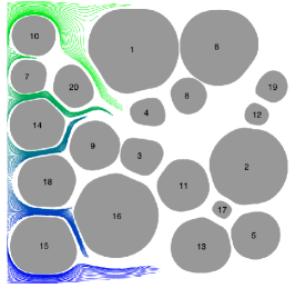
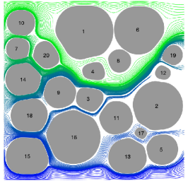
Figure 8: 200 streamlines in the second geometry from figure 6. The streamlines are initially equispaced at $(-1,y)$, where $y\in(-1,1)$. The first five snapshots are equispaced in time. The bottom right frame is a magnification of the fifth snapshot, but with additional streamlines.

In figure 6, we observe that erosion creates a network of channels from the inlet to the outlet where the velocity and vorticity, and therefore erosion rate, are much larger relative to other regions. These channels can be further visualized with the streamlines. In figure 8, we freeze the geometry at the second snapshot from figure 6 and plot 200 streamlines that are initially equispaced along $(-1,y)$, where $y\in(-1,1)$. The streamlines are shown at five different times, and the final plot is a zoom in of the lower right quadrant of the fifth time step, but with additional streamlines. Since we use a high-order quadrature rule and time stepping method, we resolve streamlines that come very close to the eroded bodies. There are three clear regions where the streamlines are most concentrated, corresponding to the regions of highest velocity. Two of these regions are located between the bodies and the solid walls at $y=\pm 1$, and the third cuts through the porous region with the upper part of the channel formed by bodies 1, 4, 6, and 8. Since the flow is fastest in these regions, the shearing is largest, and this causes the channels to continue to open fastest as observed in figure 6.

Next, we use the $N_{p}=1000$ (Bellin et al., 1992) streamlines to compute the tortuosity of the eroding geometry. To compute the tortuosity, we require the velocity at the inlet $x=-1$. These normalized velocities are plotted in figure 10(a) for the eroded geometry at porosity $\phi=62.9\%$ (figure 10(c)). The velocities are similar those of Matyka et al. (2008, see figure 4(a)), except that our cross-section, by construction, does not cut through any of the grains. Next, in figure 10(b), we plot the local tortuosity (21) by calculating the relative length of each streamline as it traverses the channel from $x=-1$ to $x=1$. The local tortuosity ranges from 1 to 1.27, meaning that one of the streamlines is 27% longer than it would have been if the grains were absent. The average streamline is 9.79% longer or equivalently the tortuosity of the geometry is $1.098$. Again, comparing the local tortuosity to Matyka et al. (2008, see figure 4(b)), the results are qualitatively similar. However, since our initial cross-section does not cut through the grains, the local tortuosity does not have any gaps. Discontinuities in local tortuosity occur when nearby streamlines diverge to circumvent a grain. In figure 10(c), we plot pairs of streamlines associated with the ten largest jumps in the local tortuosity, with each pair of corresponding streamlines plotted in the same color.

(a)

(b)

(c)

Figure 10: The local tortuosity of a porous geometry initialized with 20 grains after eroding to a porosity of 62.9%. (a) The $x$-component of the velocity at the inlet, $u_{1}(-1,y)$, normalized by its maximum velocity of $2.98\times 10^{-3}$. (b) The local tortuosity $\tau(y)$ on the cross section $x=-1$. (c) The streamlines resulting in the ten largest differences of local tortuosity between neighboring streamlines. Neighboring streamlines have the same color.

In figure 11(a), we plot the tortuosity as a function of the porosity. The initial porosity is $\phi=37.68\%$, and the initial tortuosity is $T=1.16$. The tortuosity is computed with both the length of the streamlines (22) (red stars) and using the spatial average of the velocity on an Eulerian grid (23) (blue marks). The red square corresponds to the porosity of the geometry in figure 10(c). The two tortuosity formulas give similar results, and any discrepancy can be accounted for by slow regions of recirculation and from applying quadrature to compute the tortuosity. As the bodies erode, wide channels form where streamlines undergo only minor vertical deflections, and this explains why the tortuosity eventually decreases with porosity. We computed lines of best fit using the porosity-tortuosity models (24) and found that the power law minimizes the error. The black dashed line in figure 11(a) is the line of best fit $\widehat{T}(\phi)=\phi^{-0.2064}$ with a root-mean-square error of $5.90\times 10^{-3}$. Interestingly, at the low porosities, the tortuosity initially increases. This increase occurs because in the absence of erosion (left plot in figure 6), many of the streamlines, such as those initialized between bodies 15 & 18, only perform minor deflections to pass through the narrow regions, albeit, very slowly. However, as erosion starts to open the channels, the streamlines deflect into the fast regions, such as the region above body 11, and this increases the amount of vertical deflection, and therefore the tortuosity. While this increase in tortuosity is interesting, in the next two examples we will see that the tortuosity does not initially increase.

We next use streamlines to investigate the temporal evolution of the particle spreading $\sigma_{\lambda}$. The spreading is computed for seven geometries of different porosities that are formed during the erosion process (figure 11(b)). So that the spreading reaches a statistical equilibrium, we use the reinsertion algorithm described in section 4.1 to form sufficiently long trajectories. For all the reported porosities, the particle dispersion exhibits two distinct power law regimes. Initially, the dispersion is ballistic ($\sigma_{\lambda}\sim t$) since individual fluid particles have not yet explored enough space to significantly alter their velocity. However, once the particles have been subjected to a range of velocities, their dispersion slows, and we observe super-dispersive ($\sigma_{\lambda}\sim t^{\alpha}$, $\alpha\in(1/2,1)$) behavior over at least one order of magnitude in time. Before any erosion takes place, the anomalous dispersion coefficient is $\alpha=0.56$. Then, as the grains begin to erode, the dispersion rate grows towards the ballistic regime that occurs in the absence of grains. The monotonic increase in dispersion with respect to the porosity is explained by the onset of channels where many tracers experience less variability in their velocities.

(a)

(b)

Figure 11: (a) The tortuosity of an eroding geometry initialized with 20 grains. The tortuosity is calculated using the Eulerian method (23) (blue dots) and Lagrangian method (22) (red stars). The red square corresponds to the geometry in figure 10(c). The dashed line is the line of best fit $\widehat{T}(\phi)=\phi^{-p}$ with $p=0.2064$. (b) The temporal evolution of $\sigma_{\lambda}$ at seven porosities. The dashed line has slope one and corresponds to ballistic dispersion. Asymptotically, the spreading is super-dispersive with $\sigma_{\lambda}\sim t^{\alpha}$, $\alpha\in(1/2,1)$. The dashed-dotted lines of best fit have slopes $\alpha=1.06$ ($\phi=95.10\%$), $\alpha=1.07$ ($\phi=85.09\%$), $\alpha=1.06$ ($\phi=75.15\%$), $\alpha=0.97$ ($\phi=65.09\%$), $\alpha=0.78$ ($\phi=55.10\%$), $\alpha=0.75$ ($\phi=45.08\%$), and $\alpha=0.56$ ($\phi=37.68\%$). Values greater than 1 result from using a least-squares fit for the tails of the particle spreading.

6.3 20 Bodies at a Low Porosity

We consider a second example with 20 eroding bodies, but with a smaller initial porosity. In figure 12, we plot the eroding geometry and vorticity at four evenly spaced instances in time. Initially, the smallest distance between pairs of bodies is $3.29\times 10^{-4}$, and the smallest distance between the bodies and solid wall is $4.50\times 10^{-3}$. At these distances, a resolution of approximately $N_{\mathrm{in}}=27,000$ and $N_{\mathrm{out}}=18,000$ discretization points is required to satisfy the $5h$ threshold needed for the trapezoid rule to achieve machine precision.

Figure 12: 20 bodies eroding in a Hagen-Poiseuille flow. The snapshots are equispaced in time, and the color is the fluid vorticity. In addition to the channels that develop between the bodies and the solid walls, erosion leads to two main channels through the geometry—one in the top half and one near the middle.

We compute the tortuosity using the Eulerian method (23) at each time step. The initial porosity is $\phi=30.67\%$ and the initial tortuosity is $T=1.24$. In figure 13(a), we plot the tortuosity with respect to the porosity (blue) and the line of best fit (black) using the power law $\widehat{T}(\phi)=\phi^{-0.1669}$. This model outperforms the other three models in equation (24), and its root-mean-squared error is $1.13\times 10^{-2}$. As grains erode, there is an increase in the number of streamlines that take a nearly direct path through the geometry, and this decreases the tortuosity. However, the channelization effect of erosion results in an increase in the tortuosity since the length of many of the streamlines increases when they deflect from a high porosity region (low pressure) to a low porosity region (high pressure). For this example, we see that the net effect is a decrease in the tortuosity for all time.

(a)

(b)

Figure 13: (a) The tortuosity of an eroding geometry initialized with 20 grains. When compared to the last example, the bodies are initially much closer together, and the porosity is smaller. The dashed line is the line of best fit $\widehat{T}(\phi)=\phi^{-p}$ with $p=0.1669$. (b) The temporal evolution of $\sigma_{\lambda}$ at eight porosities. The dashed line has slope one and corresponds to ballistic motion. Asymptotically, the spreading is super-dispersive with $\sigma_{\lambda}\sim t^{\alpha}$, $\alpha\in(1/2,1)$. The dashed-dotted lines of best fit have slopes $0.92$ ($\phi=95.00\%$), $0.87$ ($\phi=85.17\%$), $0.87$ ($\phi=75.10\%$), $0.91$ ($\phi=65.02\%$), $0.91$ ($\phi=55.08\%$), $0.72$ ($\phi=45.03\%$), $0.69$ ($\phi=35.05\%$), and $0.92$ ($\phi=30.67\%$).

In figure 13(b), we plot the temporal evolution of the particle spreading $\sigma_{\lambda}$. As in the last example, we analyze the spreading at several different porosities and we use the reinsertion algorithm described in section 4.1. For all the porosities, the dispersion is much closer to ballistic when compared to the results in figure 11. However, there are still clear transitions from ballistic dynamics to asymptotic super-dispersive spreading. In contrast to the higher porosity initial condition (section 6.2), at early times the erosion results in a decrease in the dispersion rate. In particular, after the first 5% of the bodies have eroded, the particle spreading transitions from $\sigma_{\lambda}\sim t^{0.92}$ to $\sigma_{\lambda}\sim t^{0.69}$. To explain this behavior, recall that anomalous dispersion is caused by tracers spending time in both the fast and slow regimes. Since the initial configuration has a reasonably uniform velocity (see figure 12), albeit a small one, the dispersion is nearly ballistic. However, as the geometry erodes, the flow becomes more intermittent, and this results in an increased anomalous dispersion rate (de Anna et al., 2013). Then, as the bodies continue to erode, the geometry channelizes, and most tracers are transported with a large velocity through the channels, again resulting in a nearly ballistic motion (Siena et al., 2019).

6.4 100 eroding bodies

As a final example, we consider 100 eroding bodies with an initial porosity near 50%. Snapshots of the configurations and vorticity are in figure 14. We compute the tortuosity using both the Lagrangian (22) and Eulerian methods (23). Therefore, we compute and plot the normalized velocity at $N_{p}=1000$ points along the inlet $x=-1$ in figure 16(a) for the eroded geometry at porosity $\phi=62.98\%$ (figure 16(c)). The initial velocity of the tracers is qualitatively similar to the 20 body example (figure 10(a)), except with additional oscillations because of the additional grains. In figure 16(b), we plot the local tortuosity by finding the length of the streamlines as they pass from $x=-1$ to $x=1$. Compared to figure 10(b), the local tortuosity is much more discontinuous. These discontinuities can be explained by examining the trajectories of tracers in figure 16(c). Here, there are many instances of nearby streamlines that are deflected apart from one another as they tend to a stagnation point in the flow, and this results in trajectories with significantly different lengths. At this porosity, one of the tracers travels 25.5% farther than it would have if the bodies had been absent, and the average tracer travelled 12% farther resulting in a tortuosity of $T=1.12$.

Figure 14: The erosion of 100 nearly touching grains in a Hagen-Poiseuille flow. The four snapshots are evenly spaced in time, and the color is the fluid vorticity. Because of the large number of bodies, erosion creates many channels connecting the inlet to the outlet.

In figure 17(a), we plot the tortuosity as a function of the porosity. The initial geometry has a porosity of $\phi=50.09\%$ and the tortuosity is $T=1.20$. The tortuosity is computed with both the length of the streamlines (22) (red stars) and using the spatial average of the velocity on an Eulerian grid (23) (blue marks). The red square corresponds to the porosity of the geometry in figure 16(c). Again, the two tortuosity formulas give similar results. For this geometry, the tortuosity decreases monotonically at almost all porosities. However, the tortuosity undergoes a sudden increase near the end of the simulation, and we have observed this behavior in other examples. The increase is caused by a single small body near the middle of the channel being completely eroded. While this results in straighter streamlines, therefore reducing $\lambda$, the horizontal flow, $u_{1}(y)$, increases since there is no longer a no-slip boundary, and this increases the tortuosity. We also compute the lines of best fit using the porosity-tortuosity models (24). The black dashed line in figure 17(a) is the line of best fit $\widehat{T}(\phi)=\phi^{-0.2459}$, with a root-mean-square error of $5.50\times 10^{-3}$. We note a slightly better root-mean-square error of $5.20\times 10^{-3}$ is possible with the model $\widehat{T}(\phi)=1-0.2631\ln(\phi)$.

(a)

(b)

(c)

Figure 16: The local tortuosity of a porous geometry initialized with 100 grains after eroding to a porosity of 62.98%. (a) The $x$-component of the velocity at the inlet, $u_{1}(-1,y)$, normalized by its maximum velocity $u_{max}=3.90\times 10^{-4}$. Note that this maximum velocity is about a order of magnitude smaller than the 20 body example in figure 10. (b) The local tortuosity $\tau(y)$ on the cross section $x=-1$. Compared to figure 10, this example has more small bodies, and this results in more discontinuities in the local tortuosity. (c) The trajectories of 200 tracers initialized at $x=-1$.

In figure 17(b), we plot the temporal evolution of the particle spreading $\sigma_{\lambda}$ at six different porosities. Again, we initially observe ballistic motion (black dashed line), and then super-dispersion. Similar to the example in figure 13(b), the asymptotic anomalous dispersion rate is not growing with the porosity. Therefore, it appears that the dispersion rate in an eroding geometry depends not only the porosity, but also the location and shape of the bodies. Finally, at the highest porosity, anomalous dispersion is only observed briefly in the time interval $(0.5,1)$, and then transitions back to a ballistic regime. Since the bodies are so small at this high porosity, after reinsertion, the streamline is not significantly deflected by any of the bodies, and this results in a ballistic regime.

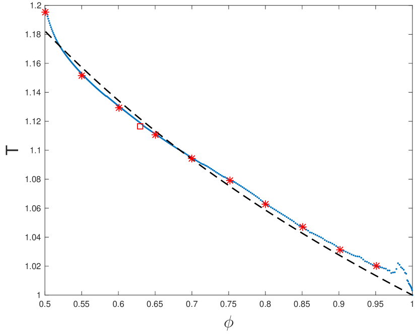
(a)

(b)

Figure 17: (a) The tortuosity of an eroding geometry initialized with 100 grains. The tortuosity is calculated using the Eulerian method (23) (blue dots) and Lagrangian method (22) (red stars). The dashed line is the line of best fit $\widehat{T}(\phi)=\phi^{-p}$ with $p=0.2459$. (b) The temporal evolution of $\sigma_{\lambda}$ at six porosities. The dashed line has slope one and corresponds to ballistic dispersion. Asymptotically, the spreading becomes super-dispersive with $\sigma_{\lambda}\sim t^{\alpha}$, $\alpha\in(1/2,1)$. The dashed-dotted lines of best fit have slopes $1.11$ ($\phi=95.12\%$), $0.68$ ($\phi=85.07\%$), $0.73$ ($\phi=75.14\%$), $0.59$ ($\phi=65.03\%$), $0.61$ ($\phi=55.02\%$), and $0.70$ ($\phi=50.09\%$).

Finally, we investigate the effect of erosion on pore sizes. The distribution of the pore sizes is directly related to the distribution of the velocity, and thus effects the tortuosity (Dentz et al., 2018) and anomalous dispersion (de Anna et al., 2018). In addition, the pore sizes are used in network models (Bryant et al., 1993b, a). As described in section 4.3, we use a Delaunay triangulation to define neighboring eroding bodies, and we compute the pore size by finding the closest distance between all neighboring bodies. Instead of computing the Delaunay configuration at each time step, which would result in new definitions for the pores at each time step, we only compute a new Delaunay triangulation when a grain completely erodes. Once all pore sizes are computed, we analyze their distribution as a function of the porosity.

In figure 18, we plot histograms of the pore pore sizes at six porosities throughout the erosion process. We superimpose the Weibull distribution (Ioannidis & Chatzis, 1993) with the same first two moments as the data. The parameters of the distribution, $(k,\lambda)$, are included in the caption of figure 18. In figure 19, we plot the mean and variance of the pore sizes as a function of the porosity. Interestingly, for porosities less than $\phi=85\%$, the mean pore size grows linearly and the variance remains nearly flat. Since a channelized geometry has large variance, this indicates that channelization is less prevalent at low porosities.

(a) 100 bodies, 258 pores

(b) 100 bodies, 258 pores

(c) 97 bodies, 249 pores

(d) 92 bodies, 234 pores

(e) 75 bodies, 189 pores

(f) 34 bodies, 74 pores

Figure 18: The pore sizes of 100 eroding bodies at six porosities. The black curves are Weibull distributions whose first and second moments agree with the data. The porosities and Weibull distribution parameters $(k,\lambda)$ at each of the porosities are: (a) $\phi=50.09\%$ and $(k,\lambda)=(1.4650,0.0605)$; (b) $\phi=55.02\%$ and $(k,\lambda)=(1.9485,0.0737)$; (c) $\phi=65.03\%$ and $(k,\lambda)=(2.5682,0.0965)$; (d) $\phi=75.14\%$ and $(k,\lambda)=(2.7771,0.1255)$; (e) $\phi=85.07\%$ and $(k,\lambda)=(2.6235,0.1713)$; (f) $\phi=95.12\%$ and $(k,\lambda)=(1.9840,0.3194)$.

(a)

(b)

Figure 19: The effect of erosion on (a) the mean and (b) the variance of the pore sizes. The geometry initially contains 100 eroding bodies. The distributions of the pore sizes in figure 18 are indicated by the red stars.

7 Conclusions

As a continuation of our previous work (Quaife & Moore, 2018), we have simulated dense suspensions and characterized transport in viscous eroding porous media. This is accomplished by using high-order time stepping methods and a new quadrature methods to solve a BIE formulation of the Stokes equations. By using these numerical methods, we are able to perform stable simulations of erosion with $N=O(100)$ discretization points, while the trapezoid rule would require $O(10^{5})$ discretization points.

The transport is characterized in terms of tortuosity and anomalous dispersion. While the local tortuosity agrees qualitatively with other works (Matyka et al., 2008), the tortuosity of eroded geometries cannot be completely described in terms of the porosity. In particular, we observe that for certain configurations, the tortuosity transiently increases, even though the porosity always increases due to erosion. We also observe super-dispersive spreading, and the rate of dispersion significantly depends not only on the porosity, but also the number of eroding bodies and their distribution.

To further our understanding of erosion, we are examining other bulk and statistical properties of an eroding porous media. In this work, we provide results for the pore throat sizes which affect the anomalous dispersion rate (de Anna et al., 2018). At a later date, we will report results on the development of anisotropic effects and the distributions of grain sizes, shapes, and opening angles.

As a long term goal, we plan to include the inertial effects and other transport models. Including inertia requires an integral equation formulation of the Navier-Stokes equations, which is an active area of research with promising directions recently proposed (Gray et al., 2019; af Klinteberg et al., 2019). Regarding other transport models, this would involve a diffusive term to consider the transport of heat or a contaminant. Forming high-fidelity simulations of such an advection-diffusion equation can be accomplished by using time splitting methods and recent work on heat solvers in complex geometries (Fryklund et al., 2019).

Acknowledgments

BQ and NM were supported by Florida State University startup funds and Simons Foundation Mathematics and Physical Sciences-Collaboration Grants for Mathematicians 527139 and 524259.

References

- Alim et al. (2017) Alim, K., Parsa, S., Weitz, D. A. & Brenner, M. P. 2017 Local Pore Size Correlations Determine Flow Distributions in Porous Media. Physical Review Letters 119, 144501.
- Allen (2019) Allen, E. J. 2019 An SDE model for deterioration of rock surfaces. Stochastic Analysis and Applications pp. 1–16.
- Alley et al. (2002) Alley, W. M., Healy, R. W., LaBaugh, J. W. & Reilly, T. E. 2002 Flow and storage in groundwater systems. Science 296 (5575), 1985–1990.
- Amin et al. (2019) Amin, K., Huang, J. M., Hu, K. J., Zhang, J. & Ristroph, L. 2019 The role of shape-dependent flight stability in the origin of oriented meteorites. Proceedings of the National Academy of Sciences 116 (33), 16180–16185.
- de Anna et al. (2013) de Anna, P., Borgne, T. Le, Dentz, M., Tartakovsky, A. M., Bolster, D. & Davy, P. 2013 Flow Intermittency, Dispersion, and Correlated Continuous Time Random Walks in Porous Media. Physical Review Letters 110 (18), 184502.
- de Anna et al. (2018) de Anna, P., Quaife, B., Biros, G. & Juanes, R. 2018 Prediction of velocity distribution from pore structure in simple porous media. Physical Review Fluids 2 (12), 124103.
- Baker & Shelley (1986) Baker, G. R. & Shelley, M. J. 1986 Boundary integral techniques for multi-connected domains. Journal of Computational Physics 64 (1), 112–132.
- Barnett et al. (2015) Barnett, A., Wu, B. & Veerapaneni, S. 2015 Spectrally-accurate quadratures for evaluation of layer potentials close to the boundary for the 2d stokes and laplace equations. SIAM Journal on Scientific Computing 37 (4), B519–B542.
- Barnett (2014) Barnett, A. H. 2014 Evaluation of layer potentials close to the boundary for Laplace and Helmholtz problems on analytic planar domains. SIAM Journal on Scientific Computing 36 (2), A427–A451.
- Beale & Lai (2001) Beale, J.T. & Lai, M.-C. 2001 A Method for Computing Nearly Singular Integrals. SIAM Journal on Numerical Analysis 38 (6), 1902–1925.
- Beale et al. (2016) Beale, J. T., Ying, W. & Wilson, J. R. 2016 A Simple Method for Computing Singular or Nearly Singular Integrals on Closed Surfaces. Communications in Computational Physics 20 (3), 733–753.
- Bear (1972) Bear, J. 1972 Dynamics of Fluids in Porous Media. New York: Dover.
- Beckermann & Viskanta (1988) Beckermann, C. & Viskanta, R. 1988 Natural convection solid/liquid phase change in porous media. International journal of heat and mass transfer 31 (1), 35–46.
- Bellin et al. (1992) Bellin, A., Salandin, P. & Rinaldo, A. 1992 Simulation of Dispersion in Heterogeneous Porous Formations: Statistics, First-Order Theories, Convergence of Computations. Water Resources Research 28 (9), 2211–2227.
- Berhanu et al. (2012) Berhanu, M., Petroff, A., Devauchelle, O., Kudrolli, A. & Rothman, D. H. 2012 Shape and dynamics of seepage erosion in a horizontal granular bed. Physical Review E 86 (4), 041304.
- Berkowitz & Scher (2001) Berkowitz, B. & Scher, H. 2001 The Role of Probabilistic Approaches to Transport Theory in Heterogeneous Media. Transport in Porous Media 42, 241–263.
- Berkowitz et al. (2000) Berkowitz, B., Scher, H. & Silliman, S. E. 2000 Anomalous transport in laboratory-scale, heterogeneous porous media. Water Resources Research 36 (1), 149–158.
- Bijeljic & Blunt (2006) Bijeljic, B. & Blunt, M. J. 2006 Pore-scale modeling and continuous time random walk analysis of dispersion in porous media. Water Resources Research 42 (1).
- Borgne et al. (2011) Borgne, T. Le, Dentz, M., Davy, P., Bolster, D., Carrera, J., de Dreuzy, J.-R. & Bour, O. 2011 Persistence of incomplete mixing: A key to anomalous transport. Physical Review E 84, 015301.
- Borgne et al. (2007) Borgne, T. Le, de Dreuzy, J.-R., Davy, P. & Bour, O. 2007 Characterization of the velocity field organization in heterogeneous media by conditional correlation. Water Resources Research 43.
- Bryant et al. (1993a) Bryant, S. L., King, P. R. & Mellor, D. W. 1993a Network model evaluation of permeability and spatial correlation in a real random sphere packing. Transport in Porous Media 11 (1), 53–70.
- Bryant et al. (1993b) Bryant, S. L., Mellor, D. W. & Cade, C. A. 1993b Physically representative network models of transport in porous media. AIChE Journal 39 (3), 387–396.
- Carman (1937) Carman, P. C. 1937 Fluid flow through granular beds. Transactions of the Institution of Chemical Engineers 15, 150–166.
- Chaoui & Feuillebois (2003) Chaoui, M. & Feuillebois, F. 2003 Creeping flow around a sphere in a shear flow close to a wall. Quarterly Journal of Mechanics and Applied Mathematics 56 (3), 381–410.
- Cho et al. (2019) Cho, H. J., Lu, N. B., Howard, M. P., Adams, R. A. & Datta, S. S. 2019 Crack formation and self-closing in shrinkable, granular packings. Soft Matter .
- Chwang & Wu (1975) Chwang, A. T. & Wu, T. Y.-T. 1975 Hydromechanics of low-Reynolds-number flow. Part 2. Singularity method for Stokes flows. Journal of Fluid Mechanics 67 (4), 787–815.
- Cushman et al. (1995) Cushman, J. H., Hu, B. X. & Deng, F.-W. 1995 Nonlocal reactive transport with physical and chemical heterogeneity:Localization errors. Water Resources Research 31 (9), 2219–2237.
- Cvetkovic et al. (1996) Cvetkovic, V., Cheng, H. & Wen, X.-H. 1996 Analysis of nonlinear effects on tracer migration in heterogeneous aquifers using Lagrangian travel time statistics. Water Resources Research 32 (6), 1671–1680.
- Dagan (1987) Dagan, G. 1987 Theory of Solute Transport by Groundwater. Annual Review of Fluid Mechanics 19, 183–215.
- Dardis & McCloskey (1998) Dardis, O. & McCloskey, J. 1998 Permeability porosity relationships from numerical simulations of fluid flow. Geophysical Research Letters 25 (9), 1471–1474.
- Dentz et al. (2011) Dentz, M., Borgne, T. Le, Englert, A. & Bijeljic, B. 2011 Mixing, spreading and reaction in heterogeneous media: A brief review. Journal of Contaminant Hydrology 120, 1–17.
- Dentz et al. (2004) Dentz, M., Cortis, A., Scher, H. & Berkowitz, B. 2004 Time behavior of solute transport in heterogeneous media: transition from anomalous to normal transport. Advances in Water Resources 27, 55–173.
- Dentz et al. (2018) Dentz, M., Icardi, M. & Hidalgo, J. J. 2018 Mechanisms of dispersion in a porous medium. Journal of Fluid Mechanics 841, 851–882.
- Duda et al. (2011) Duda, A., Koza, Z. & Matyka, M. 2011 Hydraulic tortuosity in arbitrary porous media flow. Physical Review E 84, 036319.
- Favier et al. (2019) Favier, B., Purseed, J. & Duchemin, L. 2019 Rayleigh–Bénard convection with a melting boundary. Journal of Fluid Mechanics 858, 437–473.
- Fryklund et al. (2019) Fryklund, F., Kropinski, M. C. A. & Tornberg, A.-K. 2019 An integral equation based numerical method for the forced heat equation on complex domains. arxiv 1907.08537.
- Gray et al. (2019) Gray, L. J., Jakowski, J., Moore, M. N. J. & Ye, W. 2019 Boundary integral analysis for non-homogeneous, incompressible Stokes flows. Advances in Computational Mathematics 45 (3), 1729–1734.
- Greengard & Rokhlin (1987) Greengard, L. & Rokhlin, V. 1987 A Fast Algorithm for Particle Simulations. Journal of Computational Physics 73, 325–348.
- Hakoun et al. (2019) Hakoun, V., Comolli, A. & Dentz, M. 2019 Upscaling and Prediction of Lagrangian Velocity Dynamics in Heterogeneous Porous Media. Water Resources Research 55 (5), 3976–3996.
- Helsing & Ojala (2008) Helsing, J. & Ojala, R. 2008 On the evaluation of layer potentials close to their sources. Journal of Computational Physics 227, 2899–2921.
- Hewett & Sellier (2017) Hewett, J. N. & Sellier, M. 2017 Evolution of an eroding cylinder in single and lattice arrangements. Journal of Fluids and Structures 70, 295–313.
- Hewett & Sellier (2018) Hewett, J. N. & Sellier, M. 2018 Modelling ripple morphodynamics driven by colloidal deposition. Computers & Fluids 163, 54–67.
- Higdon (1985) Higdon, J. J. L. 1985 Stokes flow in arbitrary two-dimensional domains: shear flow over ridges and cavities. Journal of Fluid Mechanics 159, 195–226.
- Hou et al. (1994) Hou, T. Y., Lowengrub, J. S. & Shelley, M. J. 1994 Removing the Stiffness for Interfacial Flows with Surface Tension. Journal of Computational Physics 114, 312–338.
- Huang et al. (2015) Huang, J. M., Moore, M. N. J. & Ristroph, L. 2015 Shape dynamics and scaling laws for a body dissolving in fluid flow. Journal of Fluid Mechanics 765.
- Ioakimidis et al. (1991) Ioakimidis, N. I., Papadakis, K. E. & Perdios, E. A. 1991 Numerical Evaluations of Analytic Functions by Cauchy’s Theorem. BIT Numerical Mathematics 31 (2), 276–285.
- Ioannidis & Chatzis (1993) Ioannidis, M. A. & Chatzis, I. 1993 Network Modelling of Pore Structure and Transport Properties of Porous Media. Chemical Engineering Science 48 (5), 951–972.
- Jambon-Puillet et al. (2018) Jambon-Puillet, E., Shahidzadeh, N. & Bonn, D. 2018 Singular sublimation of ice and snow crystals. Nature Communications 9 (1), 4191.
- Johnson & Elimelech (1995) Johnson, P. R. & Elimelech, M. 1995 Dynamics of Colloid Deposition in Porous Media: Blocking Based on Random Sequential Adsorption. Langmuir 11, 801–812.
- Kang et al. (2014) Kang, P. K., de Anna, P., Nunes, J. P., Bijelic, B., Blunt, M. J. & Juanes, R. 2014 Pore-scale intermittent velocity structure underpinning anomalous transport through 3-D porous media. Geophysical Research Letters 41, 6184–6190.
- Kang et al. (2002) Kang, Q., Zhang, D., Chen, S. & He, X. 2002 Lattice Boltzmann simulation of chemical dissolution in porous media. Physical Review E 65 (036318).
- Klages et al. (2008) Klages, R., Radons, G. & Sokolov, I. M. 2008 Anomalous transport: foundations and applications. John Wiley & Sons.
- af Klinteberg et al. (2019) af Klinteberg, L., Askham, T. & Kropinski, M. C. 2019 A Fast Integral Equation Method for the Two-Dimensional Navier-Stokes Equations. arxiv 1908.07392.
- af Klinteberg & Tornberg (2018) af Klinteberg, L. & Tornberg, A.-K. 2018 Adaptive Quadrature by Expansion for Layer Potential Evaluation in Two Dimensions. SIAM Journal on Scientific Computing 40 (3), A1225–1249.
- Klöckner et al. (2013) Klöckner, A., Barnett, A., Greengard, L. & O’Neil, M. 2013 Quadrature by expansion: A new method for the evaluation of layer potentials. Journal of Computational Physics 252, 332–349.
- Knudby & Carrera (2005) Knudby, C. & Carrera, J. 2005 On the relationship between indicators of geostatistical, flow and transport connectivity. Advances in Water Resources 28, 405–421.
- Koch & Brady (1988) Koch, D. L. & Brady, J. F. 1988 Anomalous diffusion in heterogeneous porous media. Physics of Fluids 31 (5), 965–973.
- Konikow & Bredehoeft (1978) Konikow, L. F. & Bredehoeft, J. D. 1978 Computer model of two-dimensional solute transport and dispersion in ground water, , vol. 7. US Government Printing Office.
- Koponen et al. (1996) Koponen, A., Kataja, M. & Timonen, J. 1996 Tortuos flow in porous media. Physical Review E 54 (1), 406–410.
- Kutsovsky et al. (1996) Kutsovsky, Y. E., Scriven, L. E. & Davis, H. T. 1996 NMR imaging of velocity profiles and velocity distributions in bead packs. Physics of Fluids 8 (4), 863–871.
- Lachaussée et al. (2018) Lachaussée, F., Bertho, Y., Morize, C., Sauret, A. & Gondret, P. 2018 Competitive dynamics of two erosion patterns around a cylinder. Physical Review Fluids 3 (1), 012302.
- López et al. (2018) López, A., Stickland, M. T. & Dempster, W. M. 2018 CFD study of fluid flow changes with erosion. Computer Physics Communications 227, 27–41.
- Matyka et al. (2008) Matyka, M., Khalili, A. & Koza, Z. 2008 Tortuosity-porosity relation in porous media flow. Physical Review E 78 (2), 026306.
- Miller et al. (1998) Miller, C. T., Christakos, G., Imhoff, P. T., McBride, J. F. & Pedit, J. A. 1998 Multiphase flow and transport modeling in heterogeneous porous media: challenges and approaches. Advances in Water Resources 31 (2), 77–120.
- Mitchell & Spagnolie (2017) Mitchell, W. H. & Spagnolie, S. E. 2017 A generalized traction integral equation for Stokes flow, with applications to near-wall particle mobility and viscous erosion. Journal of Computational Physics 333, 462–482.
- Moore (2017) Moore, M. N. J. 2017 Riemann-Hilbert Problems for the Shapes Formed by Bodies Dissolving, Melting, and Eroding in Fluid Flows. Communications on Pure and Applied Mathematics 70 (9), 1810–1831.
- Moore et al. (2013) Moore, M. N. J., Ristroph, L., Childress, S., Zhang, J. & Shelley, M.J. 2013 Self-similar evolution of a body eroding in a fluid flow. Physics of Fluids 25 (11), 116602.
- Morrow et al. (2019) Morrow, L. C., King, J. R., Moroney, T. J. & McCue, S. W. 2019 Moving boundary problems for quasi-steady conduction limited melting. arxiv 1901.01247.
- Nilsen & Storesletten (1990) Nilsen, T. & Storesletten, L. 1990 An analytical study on natural convection in isotropic and anisotropic porous channels. Journal of Heat Transfer 112 (2), 396–401.
- Parker & Izumi (2000) Parker, G. & Izumi, N. 2000 Purely erosional cyclic and solitary steps created by flow over a cohesive bed. Journal of Fluid Mechanics 419, 203–238.
- Power & Miranda (1987) Power, H. & Miranda, G. 1987 Second kind integral equation formulation of stokes’ flows past a particle of arbitrary shape. SIAM Journal on Applied Mathematics 47 (4), 689–698.
- Pozrikidis (1992) Pozrikidis, C. 1992 Boundary Integral and Singularity Methods for Linearized Viscous Flow. New York, NY, USA: Cambridge University Press.
- Puyguiraud et al. (2019) Puyguiraud, A., Gouze, P. & Dentz, M. 2019 Stochastic dynamics of lagrangian pore-scale velocities in three-dimensional porous media. Water Resources Research 55 (2), 1196–1217.
- Quaife & Moore (2018) Quaife, B. & Moore, M. N. J. 2018 A boundary-integral framework to simulate viscous erosion of a porous medium. Journal of Computational Physics 375, 1–21.
- Rees & Storesletten (1995) Rees, D. A. S. & Storesletten, L. 1995 The Effect of Anisotropic Permeability on Free Convective Boundary Layer Flow in Porous Media. Transport in Porous Media 19, 79–92.
- Ristroph et al. (2012) Ristroph, L., Moore, M. N. J., Childress, S., Shelley, M. J. & Zhang, J. 2012 Sculpting of an erodible body in flowing water. Proceedings of the National Academy of Sciences 109 (48), 19606–19609.
- Rycroft & Bazant (2016) Rycroft, C. H. & Bazant, M. Z. 2016 Asymmetric collapse by dissolution or melting in a uniform flow. Proceedings of the Royal Society A: Mathematical, Physical and Engineering Sciences 472, 20150531.
- Saffman (1959) Saffman, P. G. 1959 A theory of dispersion in a porous medium. Journal of Fluid Mechanics 6 (3), 321–349.
- Siena et al. (2019) Siena, M., Ilievand, O., Prill, T., Riva, M. & Guadagnini, A. 2019 Identification of Channeling in Pore-Scale Flows. Geophysical Research Letters 46 (6), 3270–3278.
- Tang et al. (2015) Tang, Y., Valocchi, A. J. & Werth, C. J. 2015 A hybrid pore-scale and continuum-scale model for solute diffusion, reaction, and biofilm development in porous media. Water Resources Research 51, 1846–1859.
- Trefethen & Weideman (2014) Trefethen, L. N. & Weideman, J. A. C. 2014 The Exponentially Convergent Trapezoidal Rule. SIAM Review 56 (3), 385–458.
- Wan & Fell (2004) Wan, C. F. & Fell, R. 2004 Investigation of Rate of Erosion of Soils in Embankment Dams. Journal of Geotechnical and Geoenvironmental Engineering 130 (4), 373–380.
- Western et al. (2001) Western, A. W., Blöschl, G. & Grayson, R. B. 2001 Toward capturing hydrologically significant connectivity in spatial patterns. Water Resources Research 37 (1), 83–97.
- Wykes et al. (2018) Wykes, M. S. D., Huang, J. M. & Ristroph, G. A. Hajjar L. 2018 Self-sculpting of a dissolvable body due to gravitational convection. Physical Review Fluids 3 (4), 043801.