Numerical and Experimental Investigation of Electro-Vortex Flow in a Cylindrical Container

Abstract

In a cylindrical container filled with an eutectic GaInSn alloy, an electro-vortex flow (EVF) is generated by the interaction of a non-uniform current with its own magnetic field. In this paper, we investigate the EVF phenomenon numerically and experimentally. Ultrasound Doppler Velocimetry (UDV) is applied to measure the velocity field in a cylindrical vessel. Second, we enhance an old numerical solver by taking into account the effect of Joule heating, and employ it for the numerical simulation of the EVF experiment. Special focus is laid on the role of the magnetic field, which is the combination of the current induced magnetic field and the external geomagnetic field. For getting a higher computational efficiency, the so-called parent-child mesh technique is applied in OpenFOAM when computing the electric potential, the current density and the temperature in the coupled solid-liquid conductor system. The results of the experiment are in good agreement with those of the simulation. This study may help to identify the factors that are essential for the EVF phenomenon, and for quantifying its role in liquid metal batteries.

1 Introduction

The object of the present study is the vortex flow that appears due to the electro-magnetic force in a cylindrical container, which is filled with the liquid metal alloy GaInSn. The considered flow is commonly known as electro-vortex flow (EVF), which develops at (or close to) a changing cross-section of a liquid conductor [1]. The changing cross-section deforms the electric currents and the distribution of the induced magnetic field and modifies, thereby, the intensity and direction of the Lorentz force. In our physical model, see Fig. 1  b, there is a sharp change of cross-section between the top copper electrode and the fluid zone (light blue colour). The arising Lorentz force is non-conservative, i.e., its curl is not equal to zero. Since such a force cannot be balanced completely by a pressure gradient, it immediately drives a fluid flow (since the EVF is not an instability, it does not need any critical threshold to set in). By comparing Fig. 1  a and Fig. 1  b, we see that this model can also be considered as the top part of a liquid metal battery (LMB) [2], in which EVFs should be considered carefully, both as a possible danger for the integrity of the liquid electrolyte [3, 4], as well as for their potentially positive role in enhancing mass transfer in the electrodes [5, 6, 7, 8]. Besides its relevance for LMBs, EVF is a well-known phenomenon in quite a number of engineering devices such as DC and AC electric arc furnaces [9], induction furnaces [10], electric jet engines [11] or pumps [12] – for an extensive overview, see [13].

In this paper, we study a paradigmatic model of an EVF, both experimentally and numerically. In our experiment, we employ (because of the opaqueness of GaInSn) Ultrasound Doppler Velocimetry (UDV) to measure the liquid metal’s velocity. As shown in Fig. 1  c, four UDV sensors (1, 3, 5, 7) are used at the same time for measuring the transient velocity of the fluid. With this non-invasive technique, we obtain detailed flow field information about the EVF, which can be processed and compared with corresponding numerical results. To conduct the numerical simulation of this EVF experiment, the solver by Weber et al. [14] was extended by considering the Joule heating effect. Just as in the previous solver, the electric potential, the current density and the temperature are solved on a parent mesh, while the other variables, such as velocity and pressure, are solved only in the fluid zone [15]. The parent mesh, however, covers all conductive parts as shown in Fig. 1  b.

The paper is structured as follows: A brief description of the experimental set-up is given in the following section. The numerical model with the employed boundary and initial conditions is discussed in section 3. Section 4 presents the numerical results and their comparison with the measured data. Some conclusions can be found in Section 5.

2 The experimental set-up

A schematic of the experimental set-up is shown in Fig. 1  b. This set-up consists of six main parts: one top cable, a top electrode, a cylindrical container filled with liquid GaInSn, a bottom electrode, a bottom cable, and a current source (not shown in Fig. 1). Note that both the top and the bottom cable are bent at a rather large distance from the vessel (appr. $1.2$ m). The lid and the side wall of the cylindrical container, whose inner radius is $R=25$ mm, are made of plastics. In order to completely fill the whole container and to avoid any air pockets, there are two inclined small holes in the cylindrical side wall, close to its connection with the top bottom of the lid. The top electrode, whose diameter is $5$ mm, has the same centre line as the lid of the container. However, the bottom electrode has the same diameter ($50$ mm) as the inner diameter of the container, so that no EVF is expected to set in there. A setup similar to our experiment was already studied experimentally using fiber-optic velocity measurement by Zhilin [16, 17]. Moreover, several theoretical [18, 19, 20, 21, 13, 22] and numerical [23, 14, 4] works of this generic geometry are available in the literature.

A DOP 3010 Ultrasound Doppler Velocimetry (UDV) from Signal-Processing was used to measure liquid metal’s velocity. Figure 1  c indicates the positions and inclinations of the holes where the UDV sensors (1, 3, 5, 7) are installed. Additionally, we measure the Earth’s magnetic field within the container (Table 1) by means of a Lakeshore Gauss meter. Figure 1  c shows the positions 2, 4, 6, 8 for the measurement of the external magnetic fields (specify model just for consistency).

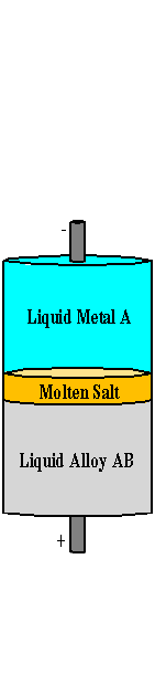
(a)

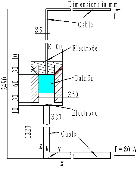
(b)

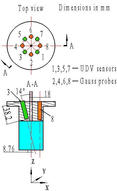
(c)

Figure 1: A schematic of an LMB (a), and the EVF experiment: (b) Sketch of the experiment. (c) Partially enlarged (1.5:1) cross-sectional view showing the distribution of the UDV sensors and the holes for the magnetic field measurements in more detail.

Table 1: The measured geo-magnetic field

Position/Mean value	$b_{x}\hskip 1.5pt$ (mT)	$b_{y}\hskip 1.5pt$ (mT)	$b_{z}\hskip 1.5pt$ (mT)
$P_{2}$	0.0144	0.0333	-0.0133
$P_{4}$	0.0164	0.0336	-0.0161
$P_{6}$	0.0152	0.0338	-0.0249
$P_{8}$	0.0146	0.035	-0.0097
Mean value	0.0151	0.0339	-0.0160

As shown in Table 1, the $b_{x}$ and $b_{y}$ values of the Earth’s magnetic fields at the different positions are almost the same. So, it seems well justified to use their average value as the external field in the entire volume of the vessel. The issue is a bit more complicated for $b_{z}$ which shows some larger deviations from its average value of $-16$ $\mu$T. Those might be attributed to some remaining permeability of the (otherwise austenitic) screws in the lid. An additional problem comes up when the current source is switched on [24]. While the arising azimuthal component of the mainly axial current can reliably be computed by Biot-Savart’s law (see next section), things are different for $b_{z}$. Various test measurements have shown that this component is not exactly zero, as it would be expected from a perfectly axial current distribution. At a current of $80$ A, the additional $b_{z}$ component is in the order of a few $\mu$T, which seems to result from field deforming effects of the contact of the upper cable to the electrodes, perhaps in combination with the mentioned permeability of the screws. Unfortunately, a precise $b_{z}$ measurement turned out to be extremely challenging, not least because of the strong geometric sensitivity of $b_{z}$ measurements in the presence of a much larger azimuthal field. Given the importance of the $b_{z}$ component in the area close to the upper lid for the formation of the EVF, we will resort to some indirect inference method, by testing numerically a variety of deviations from the observed average value of $-16$ $\mu$T.

3 Mathematical model and boundary conditions

In the mathematical model of our experimental set-up, the following assumptions are made:
1. The magnetic permeability of all parts (including air) is assumed to be the value of vacuum.
2. The two plastic parts (cylindrical rim and upper lid) are considered to be adiabatic for heat transfer.
3. The physical properties of liquid metal (viscosity, electric conductivity and thermal conductivity, etc.) are assumed to be homogeneous, isotropic and not to depend on the temperature.
The flow in an incompressible, viscous and electrically conducting fluid is described by the Navier-Stokes equation (NSE) [25]

$$\dot{\textbf{{u}}}+(\textbf{{u}}\cdot\nabla)\textbf{{u}}=-\frac{\nabla p}{\rho}+\nu\Delta\textbf{{u}}+\frac{\textbf{{f}}_{L}}{\rho}+\textbf{{f}}_{T}$$ (1)

and the continuity equation

$$\nabla\cdot\textbf{{u}}=0,$$ (2)

with u denoting the velocity, p the pressure, $\rho$ the density, $\nu$ the kinematic viscosity, $\textbf{{f}}_{L}$ the Lorentz force and $\textbf{{f}}_{T}$ the buoyancy.

The trigger of the EVF is the Lorentz force

$$\textbf{{f}}_{L}=\textbf{{J}}\times\textbf{{B}},$$ (3)

with J meaning the total current density and B the total magnetic field. Note that the total magnetic field consists of two parts: the first part is the static magnetic field $\textbf{{B}}_{0}$, generated by the applied current I (or the corresponding current density $\textbf{{J}}_{0}$); the second part is the external Earth’s magnetic field b. Although the second part (b) is rather small, it must not be neglected because this part is multiplied with the large current density $\textbf{{J}}_{0}$ and will cause swirling flow [26]. The effect of b will be discussed in the next section.

Another driving force is buoyancy [27, 28],

$$\textbf{{f}}_{T}=gh\nabla(1-\beta(T-T_{0}))$$ (4)

with $g$ denoting the standard gravity, $h$ the vertical distance from the top surface of GaInSn zone to the position where the buoyancy is computed, $\beta$ the thermal expansion coefficient, T the temperature and $\textit{T}_{0}$ the reference temperature. Commonly, if the higher temperature domain is located in the upper region, buoyancy will have no effect to fluid flow. But in our set-up, the high temperature domain is located close to the upper electrode where the current density, and hence the Joule heating is the highest. Therefore, the effect of buoyancy should be carefully considered [29]. For computing the transient temperature field, an energy equation needs to be solved [30, 31] as

$$\dot{\textit{T}}+(\textit{{u}}\cdot\nabla)\textit{T}=\nabla\cdot(\frac{\lambda}{\rho\textit{C}_{\textit{p}}}\nabla\textit{T})+\frac{1}{\rho\textit{C}_{\textit{p}}}\frac{\textbf{{J}}^{2}}{\sigma},$$ (5)

with $\lambda$ meaning the thermal conductivity, $\textit{C}_{\textit{p}}$ the constant pressure specific heat, J the current density and $\sigma$ the electrical conductivity.

The main magnetic field ($\textbf{{B}}_{0}$) can be obtained by using Biot-Savart’s law [32, 33]

$$\textit{{B}}_{0}(r)=\frac{\mu_{0}}{4\pi}\int dV^{{}^{\prime}}\frac{\textbf{{J}}(\textbf{{r}}^{\prime})\times(\textbf{{r}}-\textbf{{r}}^{\prime})}{\left|\textit{{{r}}}-\textit{{{r}}}^{\prime}\right|^{3}},$$ (6)

with $\mu_{0}$ denoting the vacuum permeability. Here, r means the local vector where $\textbf{{B}}_{0}$ is calculated, and $\textbf{{r}}^{\prime}$ is the integration coordinate, which runs through the whole domain where J exist. For obtaining J, we have to solve the Poisson-type equation for the electric potential as

$$\nabla\cdot(\sigma\nabla\varphi)=\nabla\cdot(\sigma\textbf{{u}}\times\textbf{{B}}).$$ (7)

This entire problem is then solved with the following boundary and initial conditions:
1. For the electric potential, the boundary condition at the end of the top and the bottom cable is

$$\partial\varphi/\partial\textit{{n}}=-\textit{J}/\sigma,$$ (8)

and at the insulating parts it is

$$\partial\varphi/\partial\textit{{n}}=0.$$ (9)

2. For the temperature field on the boundary surrounded by a plastic container, we assume:

$$\partial T/\partial\textit{{n}}=0,$$ (10)

on the boundary open to air (part of the top and bottom electrode) [34]:

$$T_{b}=fT_{0}+(1-f)T_{c},\quad f=(1+\frac{\lambda_{s}}{\alpha_{s}\delta})^{-1},$$ (11)

and for obtaining the absolute temperature rise conveniently, we can simply set the initial and the reference internal temperature field to $0$ in our simulations.
3. For the hydrodynamic part, no-slip boundary conditions are used at all boundaries with solid walls. This means that all velocity components are set to zero:

$$u=0,v=0,w=0.$$ (12)

Additionally, because the liquid metal is at rest before we switch on the current source, the internal field (u) can also be initialised simply as $0$. In the equations above, $\varphi$ is the electric potential, n is the normal vector at the respective wall, $T_{b}$ is the temperature on the boundary, $T_{c}$ is the temperature at each cell centre next to the boundary, $\lambda_{s}$ is the heat transfer coefficient of the copper electrodes, $\alpha_{s}$ is the heat exchange coefficient, and $\delta$ is the distance from the cell centre to the cell face centre.

For solving and updating the flow field, the PIMPLE algorithm, which combines the PISO algorithm and the SIMPLE algorithm together, is adopted to handle the pressure-velocity coupling. The Euler scheme is used for the temporal discretisation. The time step is adjusted automatically by comparing the Courant number and the magnetic diffusion Courant number with a preset value, respectively, when the current time step is finished. Therefore, it is not important how large the initial time step is set. At each time step, the solution is considered to be converged when the residual errors of the energy equation are less than $10^{-10}$, and the residual error of the momentum equation and the Poisson equation for the electric potential are less than $10^{-7}$, respectively.

4 Validation, comparison and discussion

In order to set a complete case for our simulations, a 3D geometry was built in Inventor 2016, and saved as a STL file first. Then, we used snappyHexMesh to discretise the 3D geometry up to millions of orthogonal uniform finite volumes. So, all smooth cylindrical surfaces will become small planes. A cross-section of the fluid domain is shown in Fig. 2. The relevant physical parameters used in the simulations are listed in Tab. 2. Most of the simulations (and experiments) were done with an applied current of $80$ A.

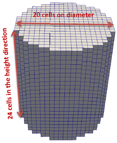
Figure 2: An example of the discretised of the fluid domain, here with the coarsest grid $20\times 24$.

Table 2: Physical parameters of liquid metal, cables and electrodes

Parameters	Value	Dimension	Region
$\rho$	6403	kg m-3
$g$	9.8	m s-2
$\lambda_{s}$	24	W (m K)-1
$\sigma$	3.3$\times 10^{6}$	S m-1	Fluid
$\mu_{0}$	1.25$\times 10^{-7}$	N A-2	(GaInSn)
$\nu$	3.4$\times 10^{-7}$	m2 s-1
$\beta$	1.2$\times 10^{-4}$	K-1
$C_{p}$	366	J (kg K)-1
$\rho$	8960	kg m-3	Cables
$\lambda_{s}$	401	W (m K)-1	and
$\sigma$	5.8$\times 10^{7}$	S m-1	Electrodes
$C_{p}$	386	J (kg K)-1

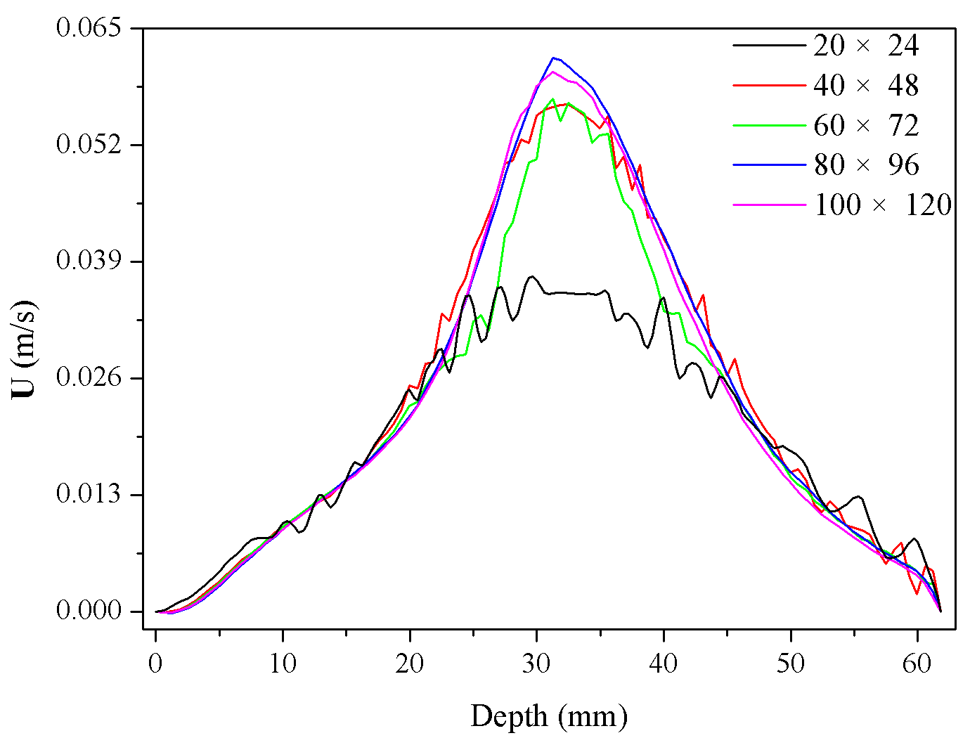
(a)

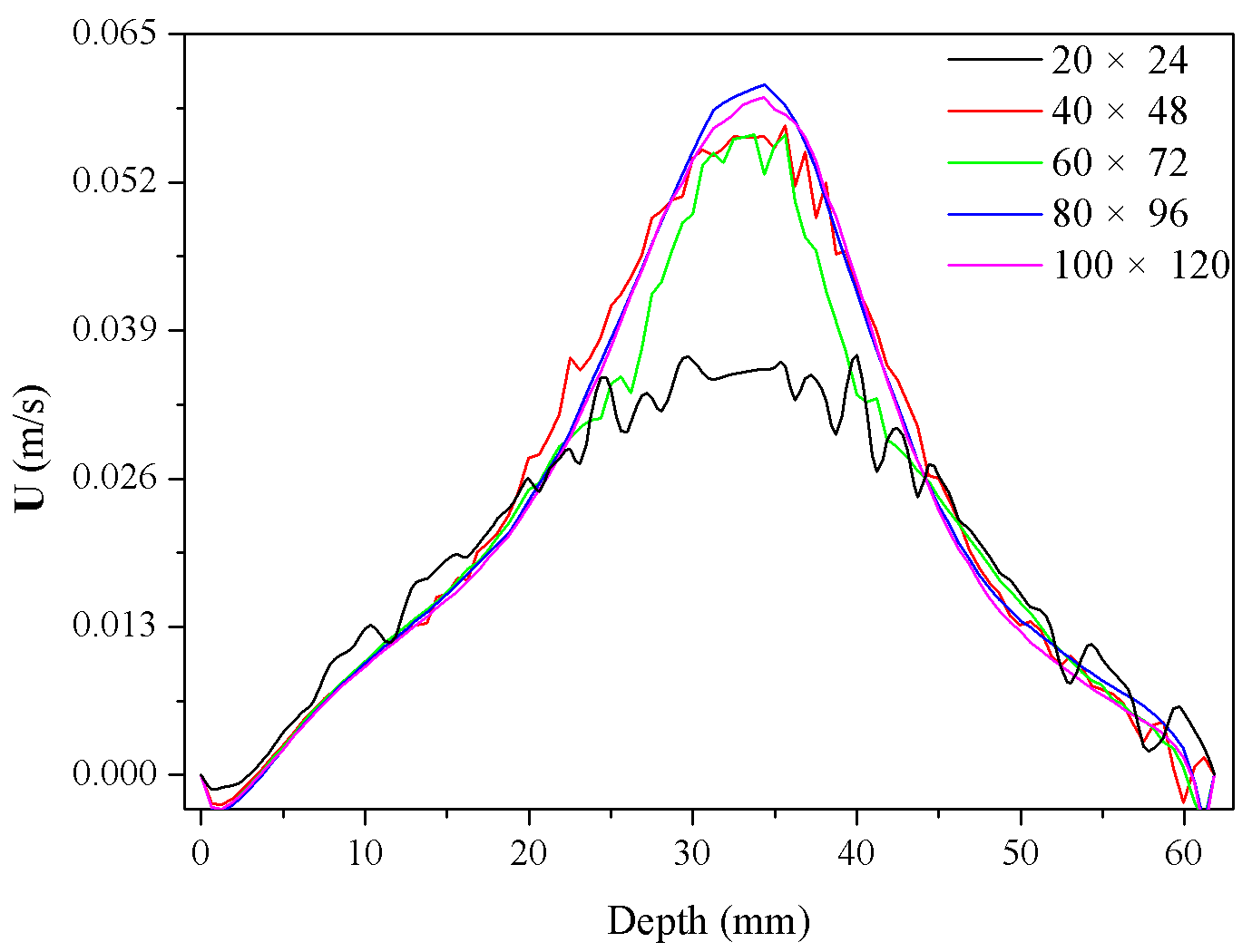
(b)

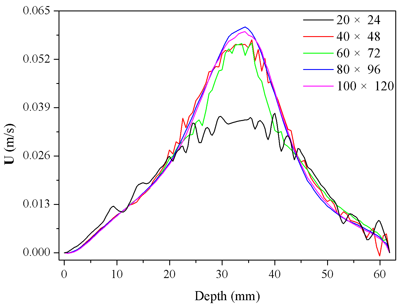
(c)

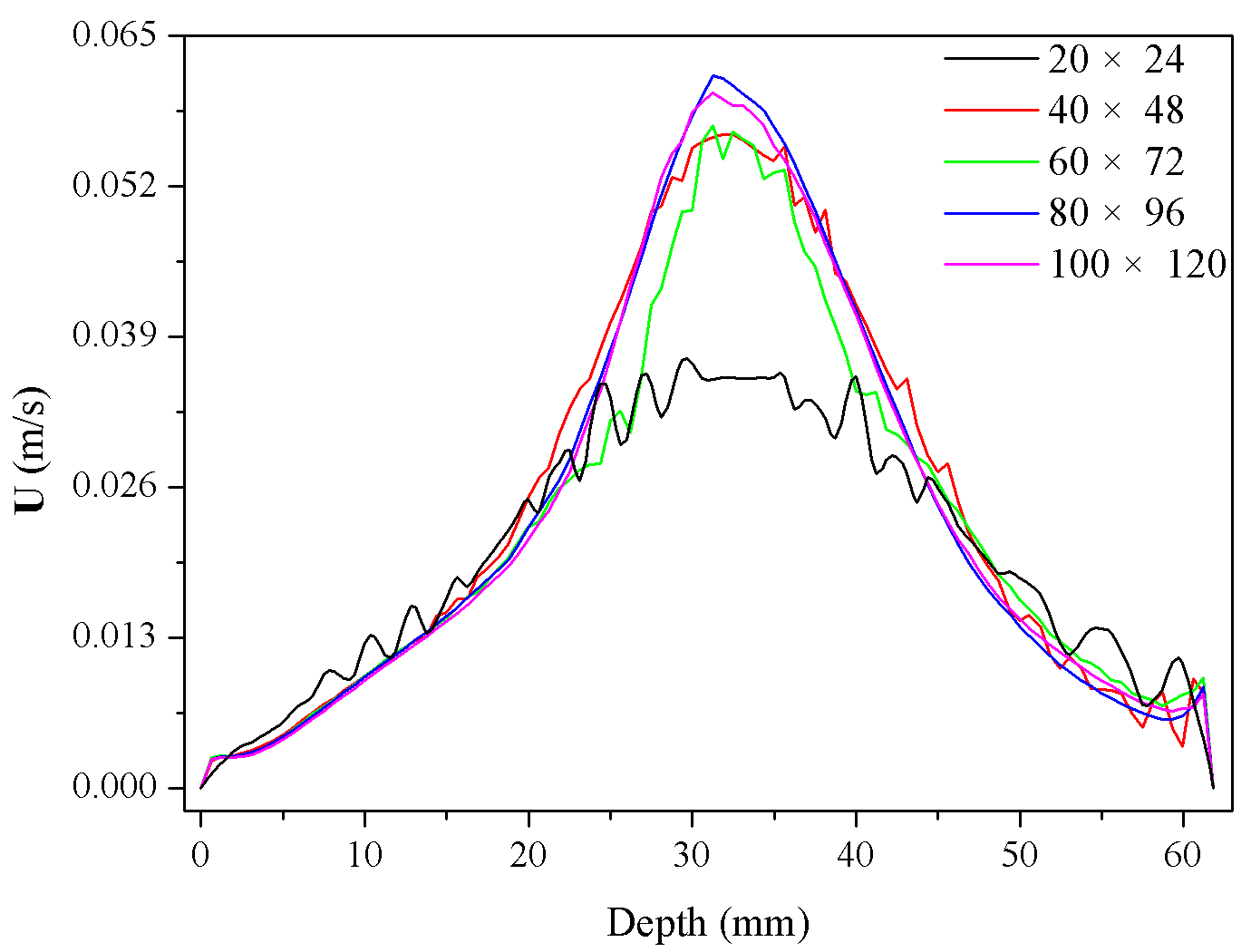
(d)

Figure 3: Distributions of velocities along the beam line of UDV sensor 1, 3, 5 and 7 with different grid sizes: (a) sensor 1, (b) sensor 3, (c) sensor 5, (d) sensor 7.

The grid independence test was performed for the case $\textit{{b}}=0$. Five different grids in the fluid region were used: $20\times 24$, $40\times 48$, $60\times 72$, $80\times 96$, $100\times 120$. Here, the first number (20, 40, 60, 80 and 100) denotes the cell number over the diameter and the second number (24, 48, 72, 96 and 120) means the cell number along the height of the fluid domain. As seen in Fig. 3, the velocity structure converges for the two highest grid resolutions, so that a grid size of $80\times 96$ is chosen for the further computations.

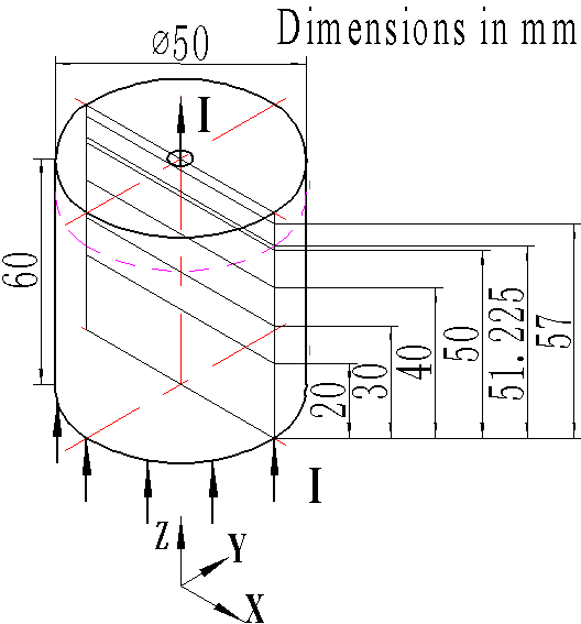
(a)

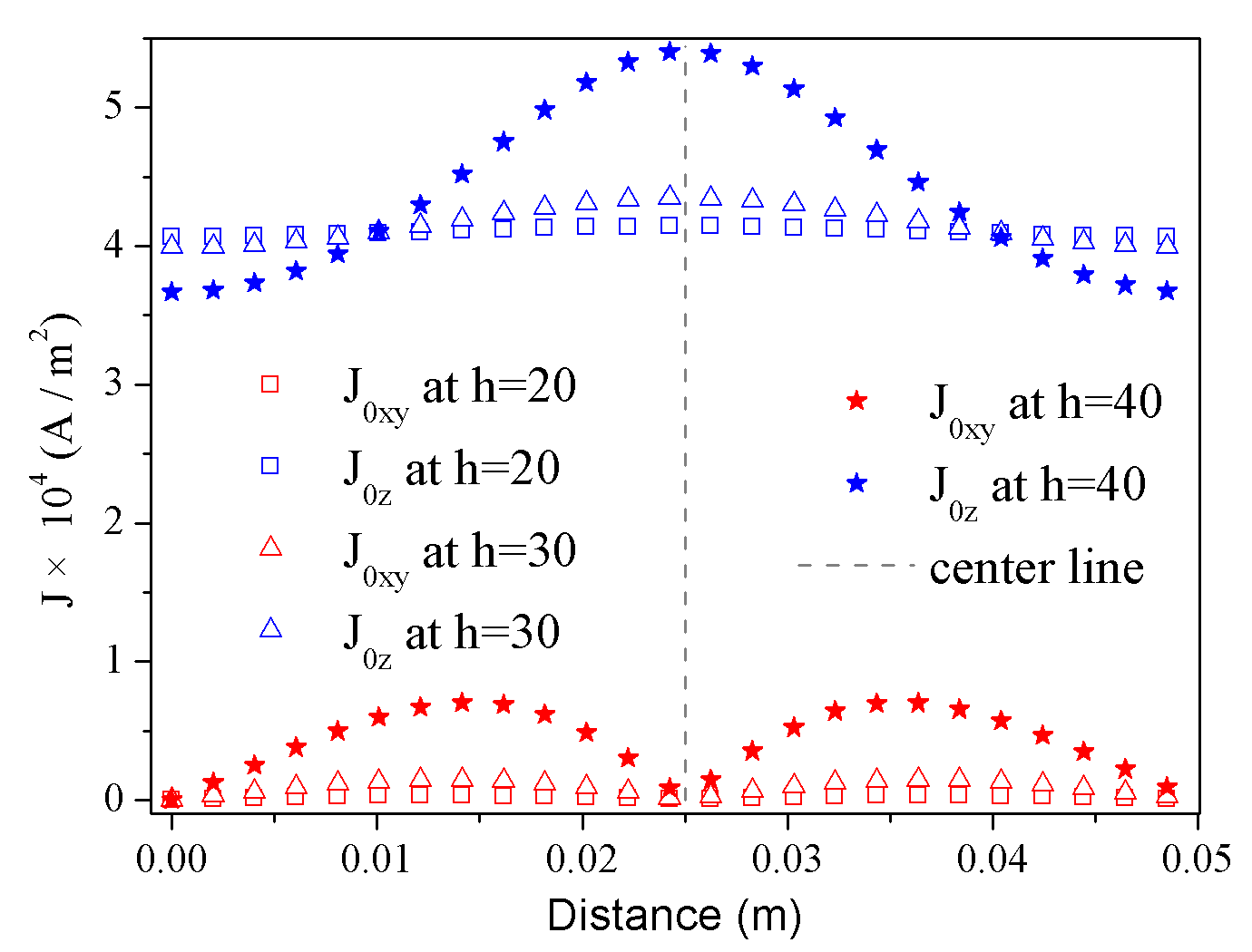
(b)

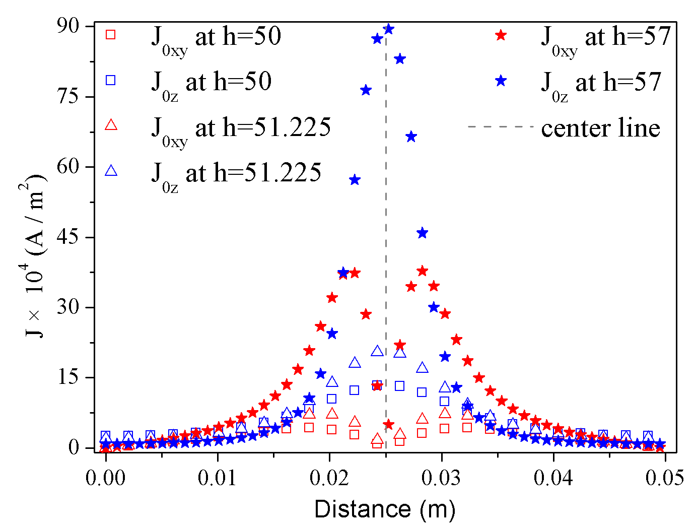
(c)

Figure 4: Current density distribution at different heights. (a) Positions where the values are sampled. (b) Distribution of current density at $h=20,30,40$ mm, respectively. (c) Distribution of current density in uppermost part of the container, at $h=50,51.225,57$ mm, respectively.

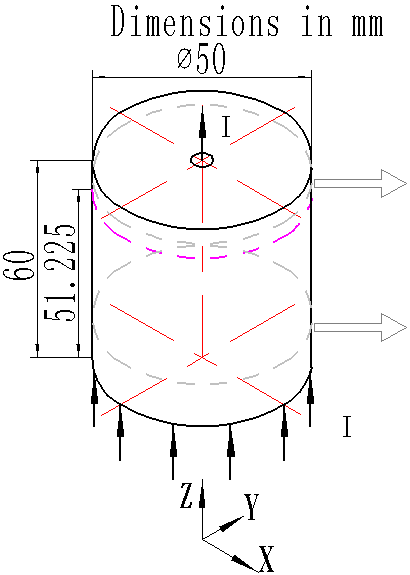
(a)

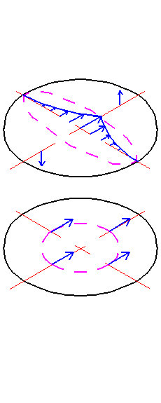
(b)

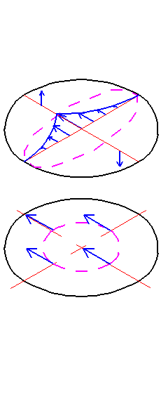
(c)

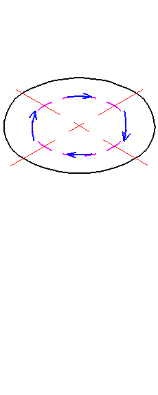
(d)

Figure 5: Schematic diagram of the distribution of the Lorentz force on different cross-sections: (a) Schematic of the fluid domain. (b) The dominant component of the Lorentz force ($J_{0}\times b_{x}$), above and below $h=51.225$ mm. (c) The dominant component of the Lorentz force ($J_{0}\times b_{y}$), above and below $h=51.225$ mm. (d) The dominant component of the Lorentz force ($J_{0}\times b_{z}$).

Figure 4 shows the distribution of the current density along the $x$ axis at different heights. As shown in Fig. 4 b and c, the cross-section at $h=51.225$ mm (indicated by the pink dashed circle in Fig. 4 a) represents a sort of a watershed, which separates the region $z<51.225$ mm, where the $z$ component of the current density is always larger than the total horizontal component from the region $z>51.225$ mm, where the $z$ component is not the dominant one.

Figure 5 shows some typical distributions of the Lorentz force on different cross-sections, as supposed to be generated by the current and one external magnetic component. Take Fig. 5 b as an example: the upper sub-plot shows the distribution of the Lorentz force on a cross-section with $z>51.225$ mm for the case of a pure $b_{x}$ field. Because in the core area $J_{0z}$ is much stronger than $J_{0xy}$, the Lorentz force points in the positive $y$ direction. However, in the surrounding area, $J_{0xy}$ is much stronger than $J_{0z}$, so the Lorentz force for $y>0$ points up, while it points down for $y<0$. The lower sub-plot illustrates the Lorentz force for $z<51.225$ mm, i.e. below the watershed, where on any horizontal cross-section $J_{0z}$ is the strongest component, so that the Lorentz force always points in positive $y$ direction. Similar effects are visible in the two sub-plots of Fig. 5 c, which illustrate the Lorentz force generated by $\textit{J}_{0}$ and a pure $b_{y}$ component. Assuming a pure $b_{z}$, Fig. 5 d shows that only a azimuthal Lorentz force can be generated. It is well known from former experiments [35, 36] and theory [20, 26, 29] that such a force drives easily an oscillating [37] or swirling flow. Considering all the three sub-plots (Fig. 5 b,c,d together, we see that the Lorentz force parts due to $b_{x}$ and $b_{y}$ can partly cancel the contribution due to $b_{z}$.

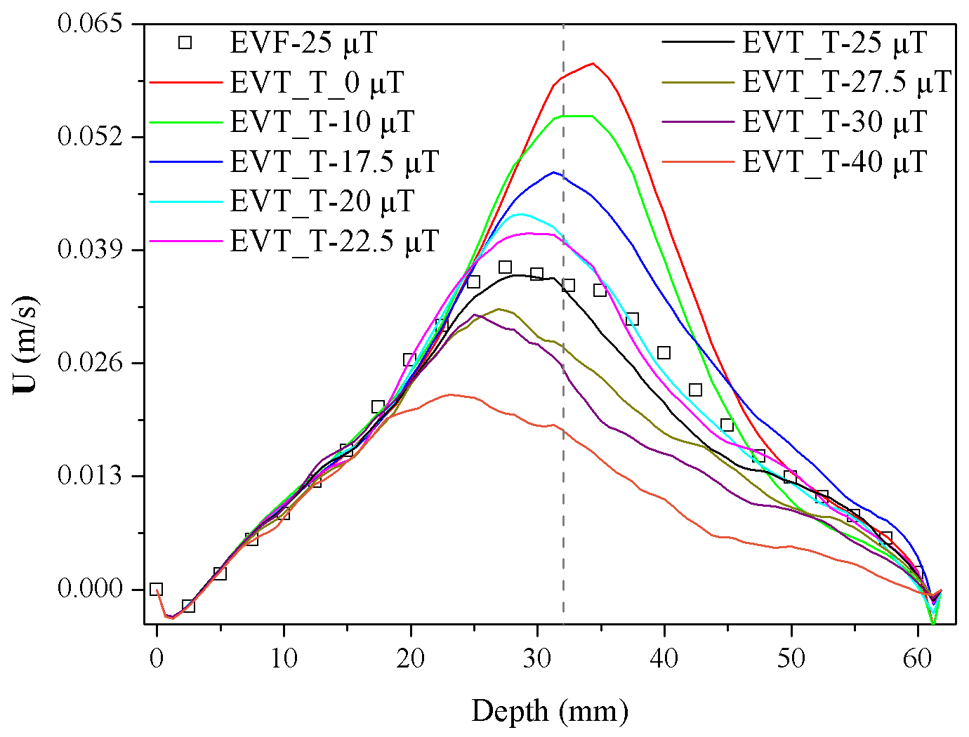
(a)

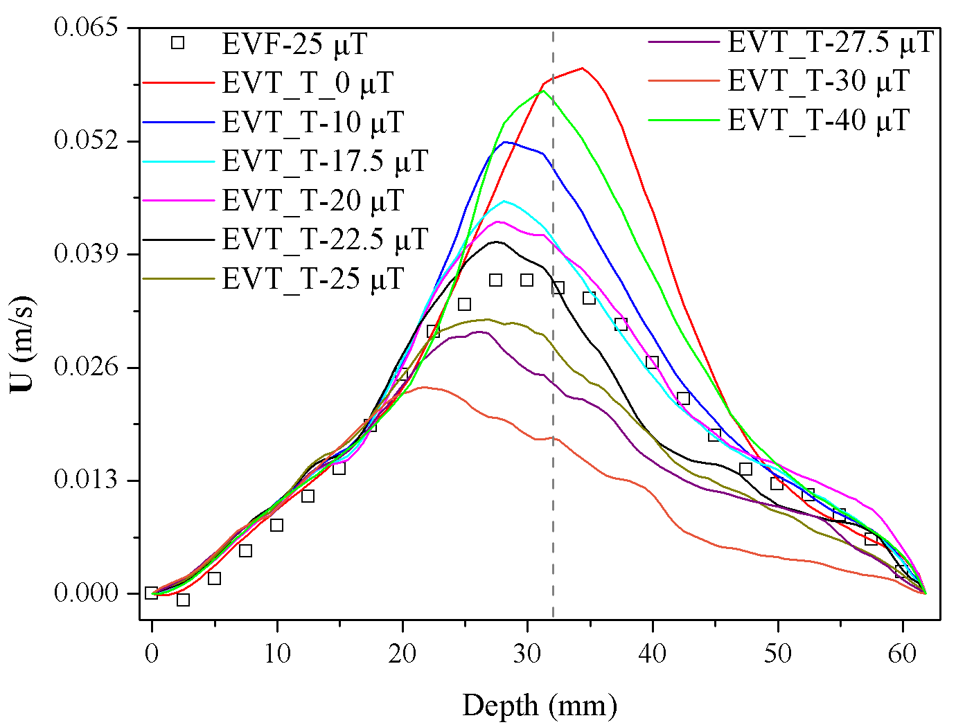
(b)

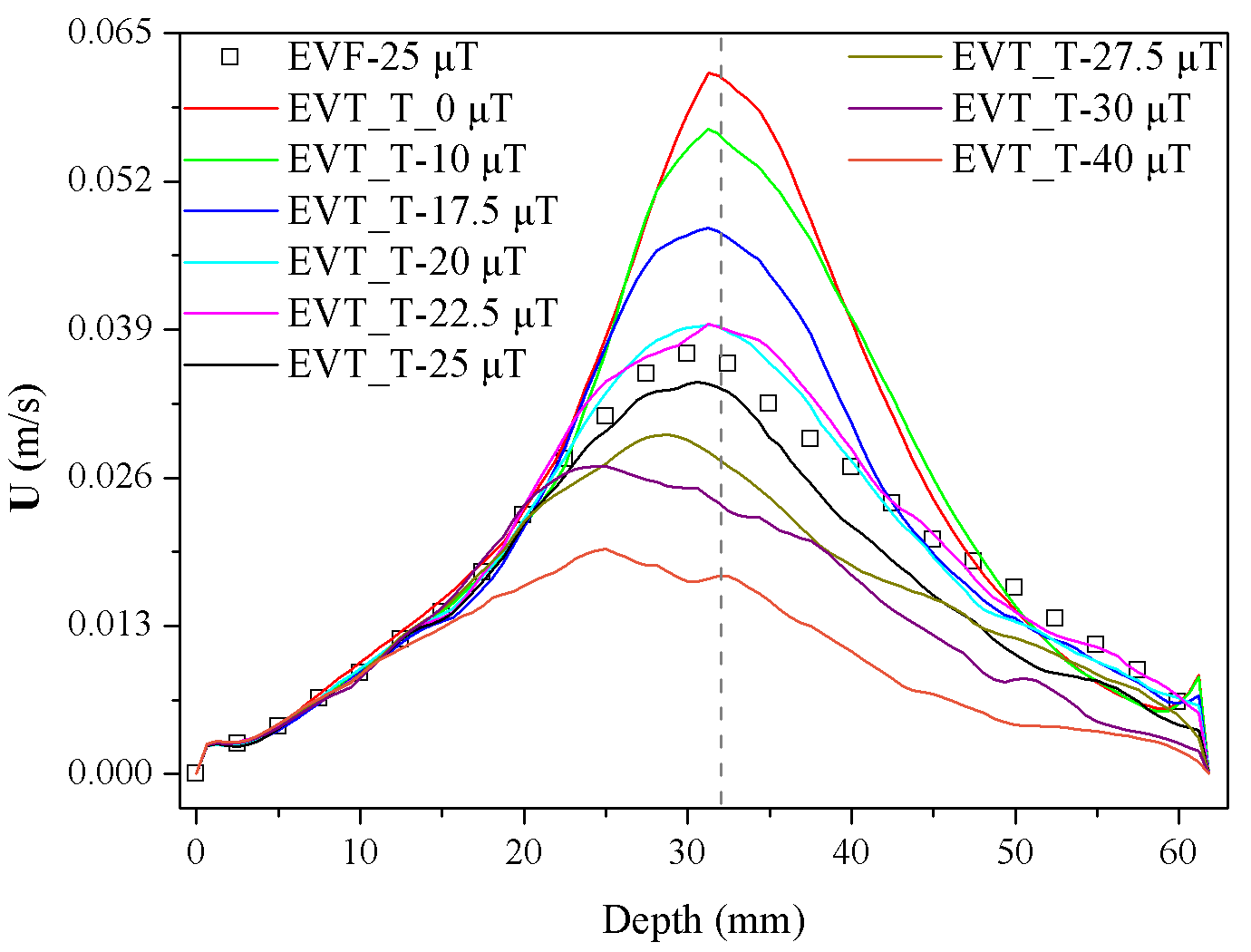
(c)

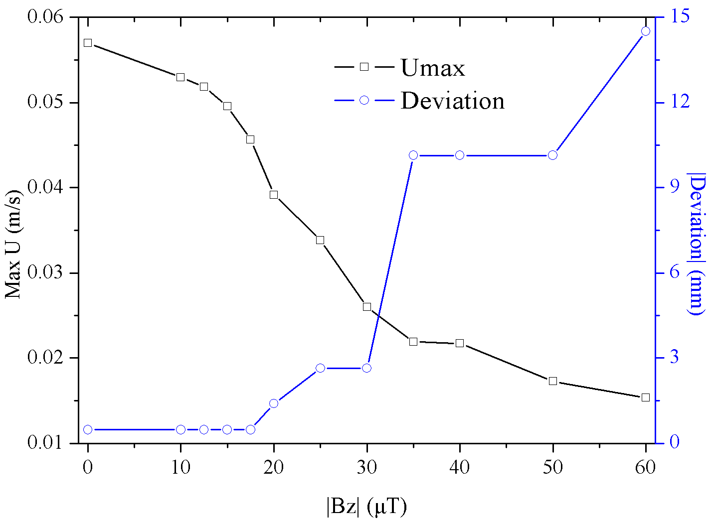
(d)

Figure 6: Distributions of velocities along the beam lines of sensor 3, 5 and 7 with different magnitudes of the external magnetic field: (a) sensor 3. (b) sensor 5. (c) sensor 7. (d) Deviation of the velocity peak from the grey dashed line, and maximum velocity for sensor 3.

We discuss now the velocity fields that result from the Lorentz forces considered above. Figure 6 shows the velocity profiles as simulated along the beam line of the UDV sensors 3, 5 and 7. The legends “EVF” and “EVF_T” indicate numerical results without and with the influence of buoyancy, respectively. Comparing the two settings, for the special case of an applied $b_{z}=-25.51$ $\mu$T and $b_{x}=b_{y}=0$, Fig. 6 b shows that the magnitudes and distributions of the velocity are slightly different. Since the actual value of $b_{z}$ in the related region close to the lid is not exactly known, we investigate here the effect of applying different values. Evidently, when we gradually vary $b_{z}$ from zero to $-40$ $\mu$T, we obtain quite different velocity distributions. Typically, with incrasing magnetic field amplitude, the simulated maximum velocity decreases, and its position moves to the left. Figure 6 d shows the maximum velocity and its deviation (the absolute value) from the centre line of the cylindrical container (gray dashed line) when $b_{z}$ varies from $0$ to $-60\;\mu$T in the simulations. We see, in particular, that the maximum velocity is drastically weakened between $b_{z}=-17.5$ $\mu$T and $-30$ $\mu$T. Further below we will suggest that the measured velocity profiles is well compatible with the presence of an $b_{z}$ at around $-25$ $\mu$T in the relevant region close to the upper electrode.

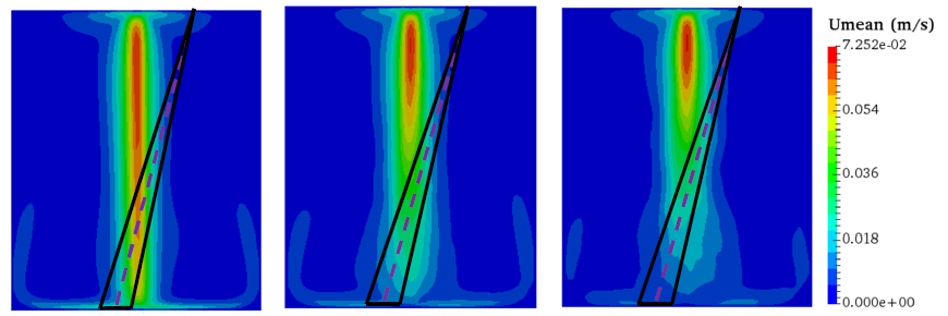
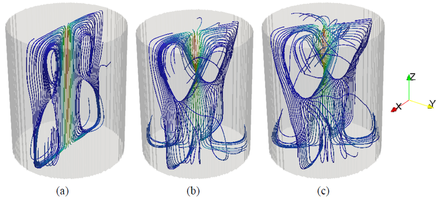
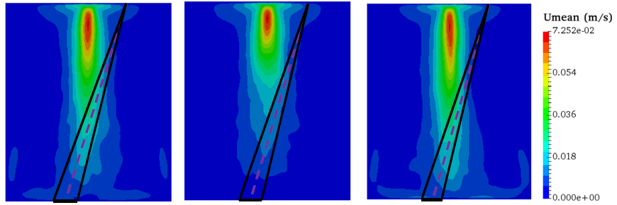
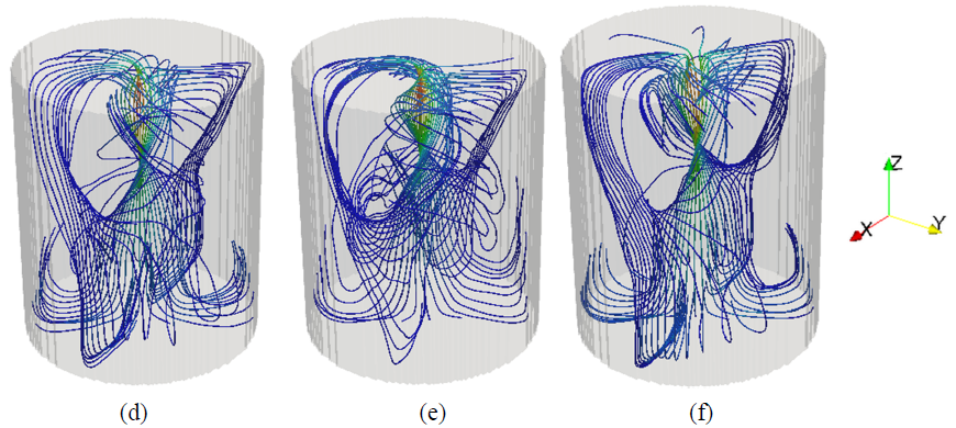
Figure 7: Velocity contours in the ZOX coordinate plane (upper sub-panels), and the corresponding streamlines (lower sub-panels), for different external magnetic field configurations: (a) $b_{z}=0$ (b) $b_{z}=-20\hskip 1.5pt\mu$T (c) $b_{z}=-25.51\hskip 1.5pt\mu$T (d) $b_{z}=-30\hskip 1.5pt\mu$T (e) $b_{z}=-40\hskip 1.5pt\mu$T (f) $b_{x}=15\hskip 1.5pt\mu$T, $b_{y}=33.9\hskip 1.5pt\mu$T, $b_{z}=-25.51\hskip 1.5pt\mu$T

Figure 7 illustrates and explains this behaviour in more detail. For different magnetic field configurations, this figure shows the time-averaged velocity contour in the ZOX coordinate plane (upper sub-panels) and the corresponding streamlines (lower sub-panels). While for $b_{z}=0$ (Fig. 7 a) the jet occupies the whole centre region down to the bottom, its length shrinks drastically when increasing the amplitude of $b_{z}$. When $b_{z}$ is enhanced from $-20$ $\mu$T to $-40$ $\mu$T (Fig. 7 b-e), the length of the jet region decreases correspondingly from about 33 percent to about 20 percent of the total height. When adding (in Fig. 7 f) some horizontal field with $b_{x}=15$ $\mu$T and $b_{y}=33.9$ $\mu$ to the $b_{z}=-25.51$ $\mu$T according to Fig. 7 c, the velocity field remains almost unchanged. Hence, for this kind of EVF, $b_{x}$ and $b_{y}$ seem to have only a minor effect on the magnitude and the distribution of the velocity field.

Note that the black triangles in Fig. 7 with purple dashed centre line indicate a conical domain where the experimental data are measured by the UDV sensor. It is obvious that this conical domain does not pass through the jet domain when the amplitude of the external magnetic field becomes stronger than $20$ $\mu$T. This explains the shifting of the ”measured” velocity towards lower depths, as seen in Fig. 6. Furthermore, the streamlines for $b_{z}=0$ are essentially 2D; when $b_{z}$ is between $-20$ $\mu$T and $-30$ $\mu$T, the two vortices at the bottom are still concentrated in the XOZ plane, while the top two vortices are already 3D-deformed gradually. For $b_{z}=-40$ $\mu$T, all four vortexes become strongly distorted.

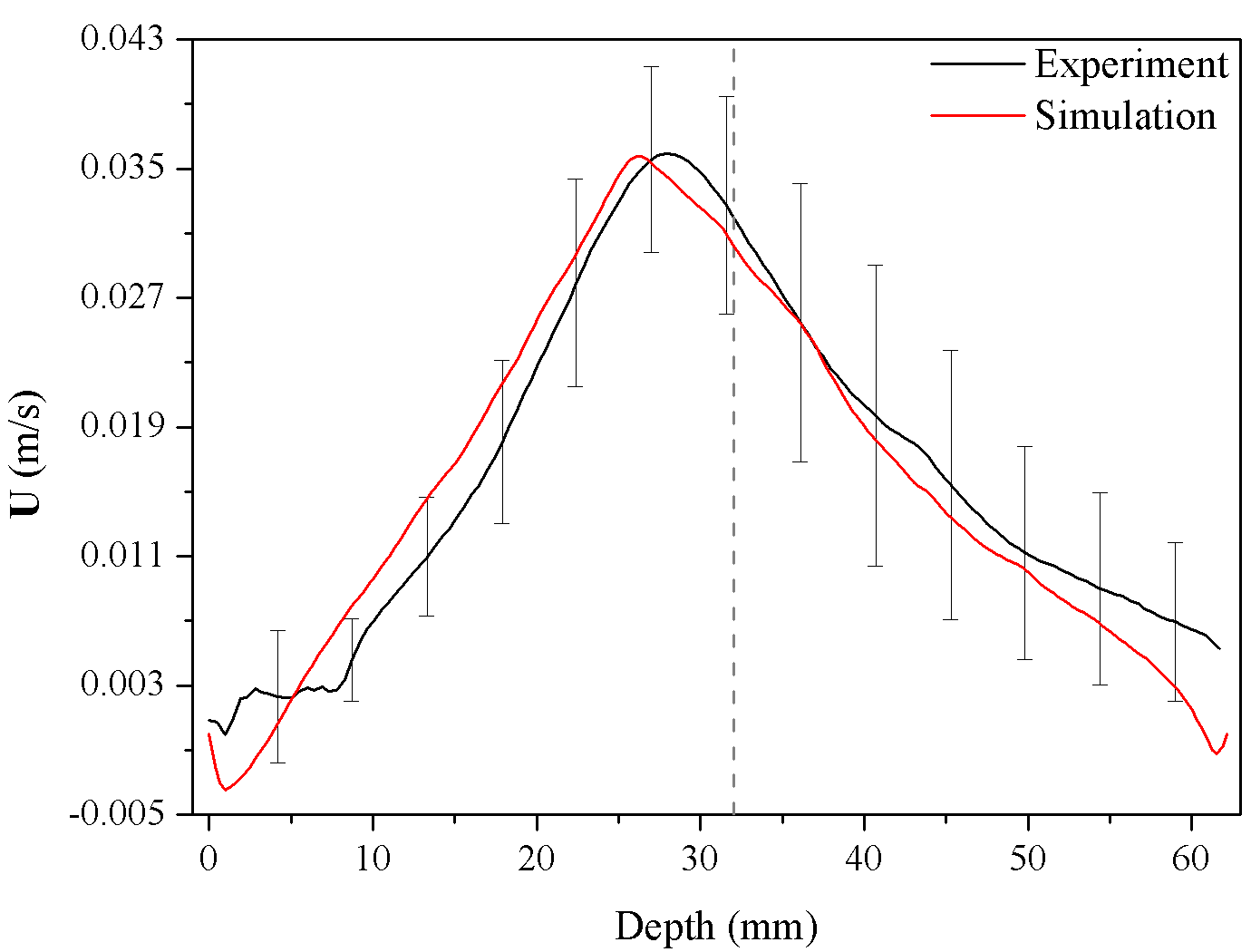
(a)

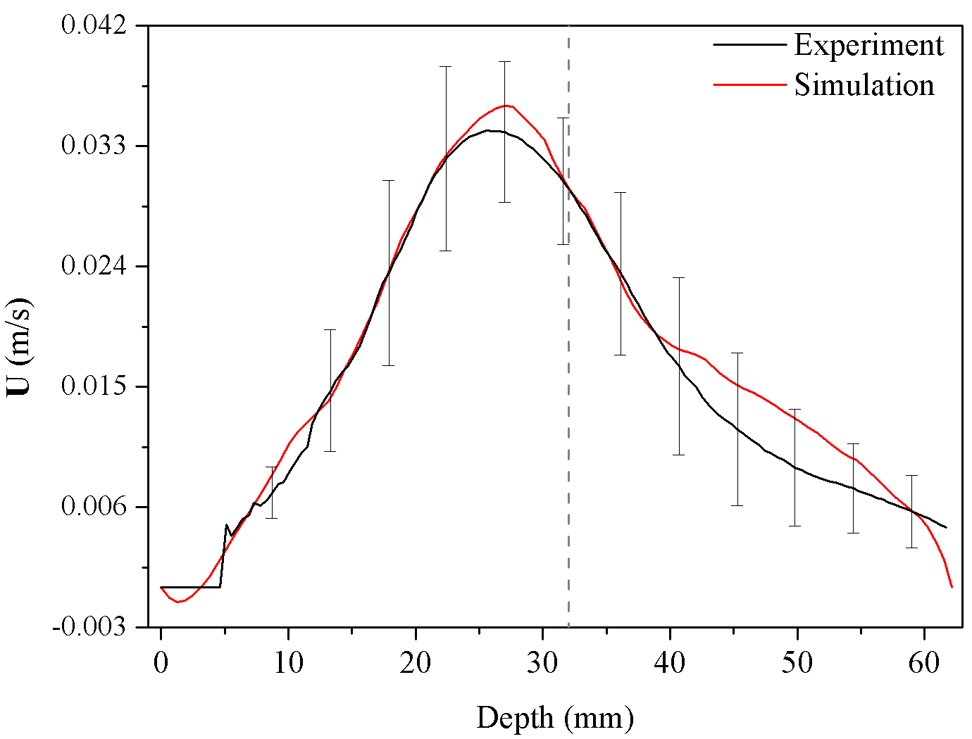
(b)

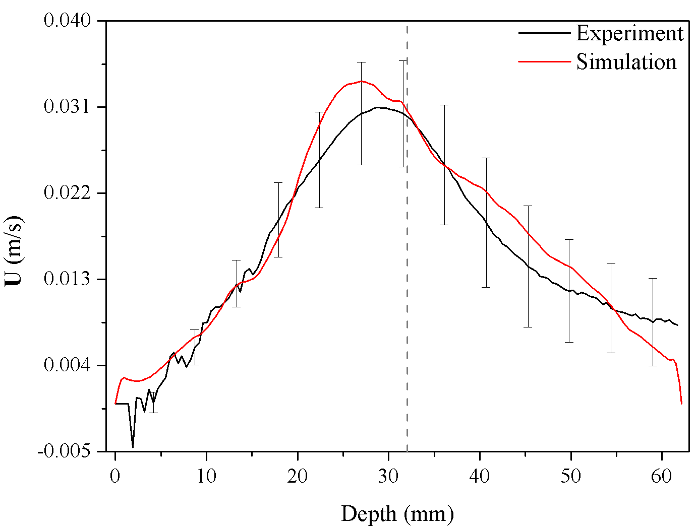
(c)

Figure 8: Comparison between numerical and experimental velocity profiles along the beams of the UDV sensors for $b_{x}=15\mu$T, $b_{y}=33.9\mu$T and $b_{z}=-25.51\mu$T: (a) sensor 3, (b) sensor 5, (c) sensor 7.

In Fig. 8, we show the velocity profiles (with error bars) as measured by UDV along the beams of three sensors (actually, the conical areas as shown in Fig. 7). The red profiles stand for numerical results sampled along the centre line of those UDV sensors, for the special case $b_{x}=15$ $\mu$T and $b_{y}=33.9$ $\mu$T, $b_{z}=-25.51$ $\mu$T (corresponding to Fig. 7 f). The comparison shows that for this assumed field configuration the numerical results nicely agree with the experiment data. As in Fig. 6, the grey dashed line in each sub-graph of Fig. 8 shows the position where the centre line of the cylindrical container crosses the centre line of the UDV beam. The high velocity domain corresponds roughly with the region of the jet. Because (with increasing $b_{z}$) the jet domain is shifted upward, the UDV beam can only pass through the bottom edge area of the high velocity domain. Again, this is the reason why the measured maximum velocity (the peaks of the profiles in Fig. 6 and Fig. 8 ) is shifted away from the centreline of the cylinder.

5 Conclusions and Outlook

In this paper, an experimental and a numerical model of the EVF in a cylindrical container have been built. First, by analysing the current distribution in the liquid metal, we have obtained numerically the Lorentz force that is responsible for generating the EVF. Second, we have found that the EVF velocity structure depends sensitively on the magnitude of the axial magnetic field $b_{z}$. Streamlines and contour graphs of the flows have revealed detailed information about the physical process that underlies this behaviour. Third, we have compared the numerical results with the experimentally measured UDV data, and found a good correspondence for an assumed $b_{z}$ of approximately $-25$ $\mu$T. This is indeed a rather plausible value, given the relativly strong variations of the measured external field from the average value of $-16$ $\mu$T, and in view of some uncertainties related to a possible effect of the current on $b_{z}$. An improvement of the experimental set-up, with a better defined and adjustable $b_{z}$, might be helpful in supporting and generalising our results. Future work will concentrate on the understanding of the time-dependence of the fluctuating jet, which becomes noticeable only for stronger $b_{z}$.

References

- [1] J. A. Shercliff. Fluid motions due to an electric current source. J. Fluid Mech., vol. 40 (1970), pp. 241–250.
- [2] N. Weber, et al. The influence of current collectors on Tayler instability and electro vortex flows in liquid metal batteries. Phys. Fluids, vol. 27 (2015), 014103.
- [3] F. Stefani, et al. Magnetohydrodynamic effects in liquid metal batteries. IOP Conf. Ser. Mater. Sci. Eng., vol. 143 (2016), 012024.
- [4] W. Herreman, et al. Numerical simulation of electro-vortex flows in cylindrical fluid layers and liquid metal batteries. Phys. Rev. Fluids, (2019), accepted.
- [5] D. H. Kelley and T. Weier. Fluid mechanics of liquid metal batteries. Appl. Mech. Rev., vol. 70 (2018), no. 2, 020801.
- [6] R. Ashour, et al. Competing forces in liquid metal electrodes and batteries. J. Power Sources, vol. 378 (2018), pp. 301–310.
- [7] T. Weier, et al. Liquid metal batteries - materials selection and fluid dynamics. IOP Conf. Ser. Mater. Sci. Eng., vol. 228 (2017), 012013.
- [8] N. Weber, et al. Electromagnetically driven convection suitable for mass transfer enhancement in liquid metal batteries. Appl. Therm. Eng., vol. 143 (2018), pp. 293–301.
- [9] O. Kazak. Modeling of Vortex Flows in Direct Current (DC) Electric Arc Furnace with Different Bottom Electrode Positions. Metall. Mater. Trans. B, vol. 44 (2013), no. 5, pp. 1243–1250.
- [10] O. V. Kazak and A. N. Semko. Numerical modeling of electro-vortical flows in a confined volume. J. Eng. Phys. Thermophys., vol. 85 (2012), pp. 1167–1178.
- [11] O. V. Kazak and A. N. Semko. Electrovortex motion of a melt in DC furnaces with a bottom electrode. J. Eng. Phys. Thermophys., vol. 84 (2011), no. 1, pp. 223–231.
- [12] S. Denisov, V. Dolgikh, S. Khripchenko, and I. Kolesnichenko. The electrovortex centrifugal pump. Magnetohydrodynamics, vol. 52 (2016), no. 1-2, pp. 25–33.
- [13] V. Bojarevičs, Y. Freibergs, E. I. Shilova, and E. V. Shcherbinin. Electrically Induced Vortical Flows (Kluwer Academic Publishers, 1989).
- [14] N. Weber, et al. Electro-vortex flow simulation using coupled meshes. Comput. Fluids, vol. 168 (2018), pp. 101–109.
- [15] S. B. Beale, et al. Open-source computational model of a solid oxide fuel cell. Comput. Phys. Commun., vol. 200 (2016), pp. 15–26.
- [16] V. G. Zhilin, et al. An experimental investigation of the velocity field in an axisymmetric electrovortical flow in a cylindrical container. Magn. Gidrodin., vol. 3 (1986), pp. 110–116.
- [17] L. A. Volokhonskii. Dynamic boundary layer of electrovortex flow in a cylindrical volume with axisymmetric current supply. Magnetohydrodynamics, vol. 27 (1991), no. 4, pp. 467–470.
- [18] I. E. Butsenieks, D. E. Peterson, V. I. Sharamkin, and E. V. Sherbinin. Magnetohydrodynamic fluid flows in a closed space with a nonuniform electric current. Magn. Gidrodin., vol. 1 (1976), pp. 92–97.
- [19] A. Y. Chudnovskii. Evaluating the intensity of a single class of electrovortex flows MHD. Magnetohydrodynamics, vol. 25 (1989), no. 3, pp. 406–408.
- [20] R. P. Millere, V. I. Sharamkin, and E. V. Shcherbinin. Effect of a longitudinal magnetic field on electrically driven rotational flow in a cylindrical vessel. Magn. Gidrodin., vol. 1 (1980), pp. 81–85.
- [21] V. K. Vlasyuk. Effects of fusible-electrode radius on the electrovortex flow in a cylindrical vessel. Magn. Gidrodin., vol. 4 (1987), pp. 101–106.
- [22] I. Kolesnichenko, S. Khripchenko, D. Buchenau, and G. Gerbeth. Electro-vortex flows in a square layer of liquid metal. Magnetohydrodynamics, vol. 41 (2005), pp. 39–51.
- [23] P. A. Nikrityuk, K. Eckert, R. Grundmann, and Y. S. Yang. An Impact of a Low Voltage Steady Electrical Current on the Solidification of a Binary Metal Alloy: A Numerical Study. Steel Res. Int., vol. 78 (2007), no. 5, pp. 402–408.
- [24] M. Starace, et al. Ultrasound Doppler flow measurements in a liquid metal column under the influence of a strong axial electric current. Magnetohydrodynamics, vol. 51 (2015), pp. 249–256.
- [25] N. Weber, et al. Numerical simulation of the Tayler instability in liquid metals. New J. Phys., vol. 15 (2013), 043034.
- [26] P. A. Davidson, et al. The role of Ekman pumping and the dominance of swirl in confined flows driven by Lorentz forces. Eur. J. Mech. - BFluids, vol. 18 (1999), pp. 693–711.
- [27] Z. Meng, et al. Code Validation for Magnetohydrodynamic Buoyant Flow at High Hartmann Number. J. Fusion Energy, vol. 35 (2016), no. 2, pp. 148–153.
- [28] H. Rusche. Computational Fluid Dynamics of Dispersed Two-Phase Flows at High Phase Fractions. Ph.D. thesis, Imperial College London, 2002.
- [29] P. Davidson, X. He, and A. Lowe. Flow transitions in vacuum arc remelting. Mater. Sci. Technol., vol. 16 (2000), no. 6, pp. 699–711.
- [30] X. H. Luo. Thermal Radiation Effects on Fluid Flow and Heat Transfer of Participating MHD in Enclosed Cavities. Ph.D. thesis, Notheast University, 2016.
- [31] P. Personnettaz, et al. Thermally driven convection in LiBi liquid metal batteries. J. Power Sources, vol. 401 (2018), pp. 362–374.
- [32] P. G. Schmidt. A Galerkin method for time-dependent MHD flow with non-ideal boundaries. Commun. Pure Appl. Anal., vol. 3 (1999), pp. 383–398.
- [33] A. J. Meir, P. G. Schmidt, S. I. Bakhtiyarov, and R. A. Overfelt. Numerical simulation of steady liquid – metal flow in the presence of a static magnetic field. J. Appl. Mech., vol. 71 (2004), no. 6, pp. 786–795.
- [34] R. Vilums. Implementation of Transient Robin Boundary Conditions in OpenFOAM. OpenFOAM workshop, 2011.
- [35] R. A. Woods and D. R. Milner. Motion in the weld pool in arc welding. Weld. J., vol. 50 (1971), pp. 163–173.
- [36] V. Bojarevičs and E. V. Shcherbinin. Azimuthal rotation in the axisymmetric meridional flow due to an electric-current source. J. Fluid Mech., vol. 126 (1983), pp. 413–430.
- [37] S. Mandrykin, I. Kolesnichenko, and P. Frick. Electrovortex flows generated by electrodes localized on the cylinder side wall. Magnetohydrodynamics, vol. 55 (2019), no. 1-2, pp. 115–123.