Anisotropic Gaussian approximation in $L_{2}(\mathbb{R}^{2})$

Abstract

Let $\mathcal{D}$ be the dictionary of Gaussian mixtures, i.e., of the functions created by all possible linear change of variables, and all possible translations, of a single Gaussian in multi-dimension. The dictionary $\mathcal{D}$ is vastly used in engineering and scientific applications to a degree that practitioners often use it as their default choice for representing their scientific object. The pervasive use of $\mathcal{D}$ in applications hinges on the scientific perception that this dictionary is universal in the sense that it is large enough, and its members are local enough in space as well as in frequency, to provide efficient approximation to “almost all objects of interest”. However, and perhaps surprisingly, only a handful of concrete theoretical results are actually known on the ability to use Gaussian mixtures in lieu of mainstream representation systems. Previous work, by Kyriazis and Petrushev, [17], and by two of us, [15], settled the isotropic case, when smoothness is defined via a Sobolev/Besov/Triebel-Lizorkin topology: it is shown in these papers that the non-linear $N$-term approximation from the dictionary $\mathcal{D}$ (and as a matter of fact from a small subset of it) is as effective as the counterpart provided by wavelets.

The present paper shows that, in 2D, Gaussian mixtures are effective in resolving anisotropic structures, too. In this setup, the “smoothness class” is comprised of 2D functions that are sparsely represented using curvelets. An algorithm for $N$-term approximation from (again, a small subset of) $\mathcal{D}$ is presented, and the error bounds are then shown to be on par with the errors of $N$-term curvelet approximation. The latter are optimal, essentially by definition. Our approach is based on providing effective approximation from $\mathcal{D}$ to the members of the curvelet system, mimicking the approach in [10, 15] where the mother wavelets are approximated. When the error is measured in the $1$-norm, this adaptation of the prior approach, combined with standard tools, yields the desired results. However, handling the $2$-norm case is much more subtle and requires substantial new machinery: in this case, the error analysis cannot be solely done on the space domain: some of it has to be carried out on frequency. Since, on frequency, all members of $\mathcal{D}$ are centered at the origin, a delicate analysis for controlling the error there is needed.

1 Introduction

1.1 The universal Gaussian mixture dictionary $\mathcal{D}$

Given the $d$-dimension Gaussian $\phi:x\mapsto e^{-|x|^{2}}$, we are interested in $N$-term nonlinear approximation from the Gaussian mixture dictionary

$$\mathcal{D}:=\{\phi\circ M\mid M\in GL(d,\mathbb{R})\ltimes\mathbb{R}^{d}\};$$

that is, a typical element of the dictionary is of the form

$$x\mapsto e^{-|A(x-k)|^{2}},$$

where $A$ is an invertible $d\times d$ matrix and $k\in\mathbb{R}^{d}$. The dictionary $\mathcal{D}$ is vast, and its members are superbly local in space as well as in frequency. It seems plausible, then, that this dictionary is universal in the sense that it provides efficient approximation to all “objects of interest”. In particular, one should expect the dictionary $\mathcal{D}$ to provide effective $N$-term approximation to functions that are smooth in the sense that they are sparsely encoded by one of the mainstream representation systems. That said, and quite surprisingly, while Gaussian mixtures are broadly used in engineering and scientific applications (including, e.g., the thousands of papers that cite either of [4], [24], or [28]), only a handful of concrete theoretical results are known about the efficacy of the dictionary $\mathcal{D}$ for $N$-term approximation.

While, as we have just alluded to above, certain theoretical aspects of Gaussian approximation are lacking, approximation by Gaussians is a common tool within Applied Mathematics. For example, it is used in scattered data approximation [27, 21, 23, 16], in PDEs (e.g., in computational chemistry [13, 20] and as Gaussian beams for time dependent problems), in other areas of numerical analysis (as shape functions for particle methods [3, 19] and as a component of the non-equispaced fast Fourier transform [12]) and in statistics (specifically in machine learning and, more specifically, in support vector machines [6, 26, 29]).

Motivated by the fact that the theoretical underpinning of the use of Gaussians in anisotropic setups is rudimentary, we focus in this paper on the utilization of $N$-term Gaussian mixtures in anisotropic setups. While we are unaware of existing results in this direction, there are related successful efforts for using Gaussians in anisotropic setups. Those, however, go beyond the mixture dictionary $\mathcal{D}$, by allowing the mixtures to be modulated: modulated, anisotropically scaled, rotated and translated Gaussians have been considered in [2, 9]. Other publications that address Gaussians in anisotropic setups include [13], where anisotropic Gaussian approximation (without rotations) has been used in very high dimensions (with the goal of obtaining dimension-independent convergence rates); [11], where surface reconstruction based on a mix of isotropic and anisotropically scaled RBFs is considered; [1], where the optimal selection of a single anisotropic dilation parameter in Gaussians SVM learning is studied, and others. In addition, anisotropic Gaussians have been used for numerical simulations in geosciences [7].

Less has been done on the utilization of Gaussians for characterizing smoothness in the ensuing $N$-term approximation schemes. An early result is Meyer’s treatment [22, Chapter 6.6] of the bump algebra $B_{1,1}^{d}(\mathbb{R}^{d})$ (consisting of infinite series of Gaussians) with wavelets. Niyogi and Girosi in [23] give rates for $N$-term approximation by isotropic Gaussian for functions in a nearby space (similar to $B_{1,1}^{d}(\mathbb{R}^{d})$). The general isotropic setup in $d$-dimensions, when smoothness is defined via a Sobolev/Besov/Triebel-Lizorkin topology was treated by Kyriazis and Petrushev, [17], and by two of us, [15]. It is shown in these papers that the non-linear $N$-term approximation from the dictionary $\mathcal{D}$ (and as a matter of fact from a small subset of it) is as effective as the counterpart provided by wavelets.

1.2 Treating anisotropic setups: our main results

We study in this paper the utility of the “universal Gaussian mixture dictionary” $\mathcal{D}$ in the representation of anisotropic 2D objects. Our “smoothness classes” are defined as sets of functions that are sparsely represented by curvelets. However, our results easily extend to smoothness classes defined via alternative anisotropic systems (e.g., shearlets, or other parabolic molecules): such extension is readily possible using the machinery and the results that were developed and established by Grohs and Kutyniok [14].

It should be stressed that we do not develop a new, Gaussian-based, representation system in this paper. Rather, we describe directly an algorithm for $N$-term approximation using members of the Gaussian dictionary $\mathcal{D}$. In this sense, our results here are essentially different from those that have been established recently by de Hoop, Gröchenig and Romero in [9]. Indeed, while [9] resolves similar classes of anisotropic objects, its setup differs from ours in two substantial aspects. First, the Gaussians in [9] are modulated, and therefore the representation in [9] employs functions that are outside our “universal” $\mathcal{D}$. Second, the focus in [9] is not on $N$-term approximation but on the construction of a representation system (a frame), with the $N$-term approximation schemes derived from the frame construction via standard arguments.

We describe now our setup and approach, and state our main result. At this introductory level, we assume the reader to have a passing familiarity with the curvelet system developed by Candès and Donoho [5]. In the interest of being self-contained, we have included the relevant technical details of the curvelet construction later on in the body of our paper.

Given $\alpha>1/2$, our curvelet-based smoothness space is comprised of functions that are defined as follows. Given $f\in L_{2}(\mathbb{R}^{2})$, we expand $f=\sum_{n=1}^{\infty}\omega_{n}\gamma_{n}$ in a decreasing rearrangement curvelet series, i.e., $(\gamma_{n})_{n\in\mathbb{N}}$ are members of the curvelet system, and $|\omega_{n}|\geq|\omega_{n+1}|$ for all $n\in\mathbb{N}$. Then our smoothness class $\mathcal{C}_{\alpha}$ is defined by

$$f\in\mathcal{C}_{\alpha}\iff|\omega_{n}|=\mathcal{O}(n^{-\alpha}).$$

The assertion in the theorem below deals with the efficient resolution of $f\in\mathcal{C}_{\alpha}$ by Gaussian mixtures. Our techniques and results, however, extend to other, related, smoothness classes. For example, we discuss (below, after the theorem) the cartoon class of Donoho and Candès. This class, to recall, consists of functions of the form $F=f_{1}+f_{2}\chi_{\Omega}$, with $f_{1}$ and $f_{2}$ both functions in $C^{2}$ and $\Omega$ is a compact set with $C^{2}$ boundary. This class enjoys a slightly different decay property of the curvelet coefficients; namely, $|\omega_{n}|=\mathcal{O}(n^{-3/2}|\log n|^{3/2})$, (see [5, Theorem 1.2]). We will come back to this cartoon class after stating our main result.

Theorem 1.

For $\alpha>1/2$, $f\in\mathcal{C}_{\alpha}$ and any $N\in\mathbb{N}$, there exists a Gaussian mixture with $N$ components, $\mathcal{T}_{N}f=\sum_{j=1}^{N}a_{j}G_{j}$ (with $G_{j}\in\mathcal{D}$ for each $j$), such that

$$\|\mathcal{T}_{N}f-f\|_{2}\leq C_{f}{N}^{\frac{1}{2}-\alpha}.$$

The constant $C_{f}$ depends on $f$ (and on $\alpha$), but is independent of $N$.

This result should be compared with $N$-term approximation by the curvelets themselves. For $f=\sum_{n=1}^{\infty}\omega_{n}\gamma_{n}\in\mathcal{C}_{\alpha}$ as above, the $N$-term approximant that is obtained by simple thresholding, viz., $\sum_{n=1}^{N}\omega_{n}\gamma_{n}$, has its error bounded by a constant multiple of $\left(\sum_{n=N+1}^{\infty}\omega_{n}^{2}\right)^{1/2}\leq CN^{\frac{1}{2}-\alpha}$.

An analogous result for the cartoon class can then be easily attained. In that case, the curvelet $N$-term approximation is of error $\mathcal{O}(N^{-1}(\log N)^{1.5})$, [5, Theorem 1.3]. Our result for an $N$-term Gaussian mixture is $\mathcal{O}(N^{-1}(\log N)^{1.5})$ as well (see our remark in section 3.1).

1.3 Our Algorithm

Our approximation scheme consists of two main components: a high order Gaussian approximant for individual curvelets, and a budgeting strategy which details the number of Gaussians that are used in our approximation of the individual curvelets in $\mathcal{D}$.

Step I: Approximation of individual curvelets. This is auxiliary, and is independent of $f$ and $\alpha$. In that step, we develop approximation schemes by Gaussian mixtures for the elements $\gamma$ of the curvelet system itself: given a curvelet $\gamma$ and a ‘budget’ of $M$ Gaussians, we provide in the first step an approximant $G_{\gamma,M}$ for $\gamma$. The approximant is a Gaussian mixture with $M$ Gaussians, i.e., a linear combination of $M$ members from the dictionary $\mathcal{D}$. This step is facilitated by the following crucial fact: the curvelet system is obtained by applying certain unitary operations to a smaller number of prototypes. The Gaussian mixture dictionary is invariant under these unitary operations. Thus, if $\gamma=U\gamma^{\prime}$, where $\gamma$ is a curvelet, $\gamma^{\prime}$ the corresponding curvelet prototype, and $U$ the unitary transformation, then we define

$$G_{\gamma,M}:=UG_{\gamma^{\prime},M},$$

and reduce in this way the problem to finding effective approximations for the prototypes themselves.

Step II: Budgeting. We assemble the $N$-term approximation, $\mathcal{T}_{N}f$, for $f$, from suitable approximations, $G_{\gamma,M}$, to the underlying curvelets. We first expand $f$, as before, in its decreasing rearrangement:

$$f=\sum_{n=1}^{\infty}\omega_{n}\gamma_{n}.$$

Then, once $N$ is given, our goal is to approximate $f$ by a mixture $\mathcal{T}_{N}f$ of $N$ Gaussians. To this end, we partition our budget $N$ of Gaussians into

$$N=\sum_{n=1}^{\infty}N(n),$$

of non-negative sub-budgets. We note that the above decomposition of $N$ is universal: it does not depend on $f$ and it does not depend on $\alpha$. Specifically, if $N(n)\not=0$, one of the possible budgeting algorithms in this paper takes the form

$$N(n)=\left\lfloor\frac{\sqrt{2}}{2}\sqrt{\frac{N}{m_{n}}}\right\rfloor,$$

with $m_{n}=2^{\lceil\log_{2}(n)\rceil}$. For example, if $N=256$, then the first few terms in the sequence $(N(n))_{n}$ are

$$(11,8,5,5,4,4,4,4,\ldots).$$

For those values $N(n)$ which exceed a threshold $N_{0}$ (which is the minimum number of Gaussians we use for approximating any curvelet), we approximate the curvelet $\gamma_{n}$ by a mixture $G_{\gamma_{n},N(n)}$ using the method that is discussed in Step I.

The approximation scheme: Given a function $f\in\mathcal{C}_{\alpha}$, and an integer $N$, we construct the Gaussian mixture $\mathcal{T}_{N}f$ from Theorem 1 by employing the two steps described above:

$$\mathcal{T}_{N}f:=\sum_{n}\omega_{n}G_{\gamma_{n},N(n)},$$

with the summation being over all the terms that are approximated. Since the sub-budgets $(N(n))_{n}$ are non-increasing, we always approximate the head of the series

$$f=\sum_{n=1}^{\infty}\omega_{n}\gamma_{n},$$

and exclude from the approximation the tail of that series. Moreover, since the sub-budgets $N(n)$ depend only on $N$, the number of curvelets that we approximate depends also only on $N$. The scheme $\mathcal{T}_{N}$, however, is non-linear: the non-linearity is due here to the fact that the $n$th curvelet $\gamma_{n}$ in the rearranged series depends on the function $f$, hence the actual curvelets that are approximated are $f$-dependent.

1.4 Organization

The paper is structured as follows. In section 2, we present some background material on the curvelet system, a more technical overview of the $N$-term approximation algorithm, and a more precise statement of the main theorem. We also state two lemmas, Lemma 3 and Lemma 5, that are pillars in the proof of the theorem.

Section 3 contains the proof of the theorem. More precisely, it shows how to invoke Lemmas 3 and 5 in order to yield the result, but does not contain the proofs of the lemmas.

Lemma 3, which describes how the approximation of individual curvelets (Step I in the algorithm) is carried out, is proved in section 4.

Lemma 5, which shows, roughly, that the system of individual errors forms a Bessel system (which is an exceptionally subtle fact) is proved in section 5. Our proof of this fact uses the theory of generalized shift invariant systems (GSI theory); the argument also incorporates ideas from the recent work of de Hoop, Gröchenig, and Romero [9] (indeed, a key technical result, specific to working with the curvelet system, has been adapted from their paper – see Lemma 15 below).

The Appendix contains a technical construction of the curvelet system; the latter details are needed for the proofs in section 5.

2 Algorithm and main results

2.1 Basics on curvelets

In this section, we outline some relevant details on curvelets. More specific details are collected in Appendix A. Our source for this “background curvelet material” is [5].

We denote the curvelet dictionary by $\mathcal{D}_{curv}$. This is a countable subset of the Schwartz space $\mathcal{S}(\mathbb{R}^{2})$. Moreover, each curvelet is band-limited; $\mathcal{D}_{curv}$ is a tight frame for $L_{2}(\mathbb{R}^{2})$.

A given curvelet $\gamma\in\mathcal{D}_{curv}$ is associated with an index vector $\mu:=\mu(\gamma)$. The index $\mu(\gamma)$ is a triplet: $\mu=(\mu(1),\mu(2),\mu(3))=:(j(\gamma),\ell(\gamma),k(\gamma))$ – it determines the scale $j:=j(\gamma)$, the orientation $\ell:=\ell(\gamma)$, and the placement $k:=k(\gamma)$ of the curvelet $\gamma$ in $\mathbb{R}^{2}$.

The curvelets from a single, fixed, scale level $j$ are generated by suitable unitary operations applied to a single prototype curvelet $\bm{\gamma}^{(j)}$ (which we call, once the scale $j$ is fixed, the curvelet generator, for the curvelets in that scale). Each generator $\bm{\gamma}^{(j)}$ is a band-limited Schwartz function with non-negative Fourier transform. The two other entries in $\mu(\gamma)$, for a curvelet $\gamma$ at scale $j$, are the rotation parameter $\ell$ that varies over the integers in $[0,2^{\lfloor j/2\rfloor}-1]$, and the translation parameter $k$ that varies over a $j$-dependent lattice $\mathbb{X}_{j}\subset\mathbb{R}^{2}$:

$$\mathbb{X}_{j}=\left\{\left(\frac{k_{1}}{\Lambda_{j}},\frac{k_{2}}{\lambda_{j}}\right)\mid(k_{1},k_{2})\in 2\pi\mathbb{Z}^{2}\right\},$$ (1)

and where $\Lambda_{j}={\varepsilon_{1}(j)2^{j}}$, $\lambda_{j}=\varepsilon_{2}(j)2^{\lfloor{j}/2\rfloor}$ are $j$ dependent lattice constants. The curvelet $\gamma$ has the form

$$\gamma:x\mapsto{|D_{\gamma}|}^{1/2}\bm{\gamma}^{(j)}\bigl{(}D_{\gamma}(R_{\gamma}^{*}x-k(\bm{\gamma}))\bigr{)},\quad x\in\mathbb{R}^{2}.$$ (2)

Here, $D_{\gamma}$ is a dilation operator and $R_{\gamma}$ is a rotation operator (as is $R_{\gamma}^{*}=R_{\gamma}^{-1}$, naturally): specifically, $D_{\gamma}$ is the parabolic scaling matrix

$$D_{\gamma}:=\begin{pmatrix}2^{j(\gamma)}&0\\ 0&2^{\lfloor j(\gamma)/2\rfloor}\end{pmatrix},$$

and $R_{\gamma}$ is a counter-clockwise rotation by the angle $\pi\ell(\gamma)\,2^{-\lfloor j(\gamma)/2\rfloor}$. We occasionally use the notation $D_{j}$ (with $j:=j(\gamma)$) in place of $D_{\gamma}$, and use $R_{j,\ell}$ or $R_{\mu}$ in place of $R_{\gamma}$ (with $\mu:=\mu(\gamma)=:(j,\ell,...))$.

We make frequent use of the following two facts

• The map $\mu:\mathcal{D}_{curv}\to\{(j,\ell,k)\mid j\in\mathbb{N},\ \ell\in\{0,\dots,2^{\lfloor j/2\rfloor}-1\},\ k\in\mathbb{X}_{j}\}$ from curvelets to their indices is a bijection.

• Every curvelet is obtained from its generator via a unitary transformation: $\gamma=U_{\gamma}\bm{\gamma}^{(j)}$ where $U_{\gamma}:L_{2}(\mathbb{R}^{2})\to L_{2}(\mathbb{R}^{2})$ is the unitary operator defined as

  $$U_{\gamma}:F\mapsto{|D_{\gamma}|}^{1/2}F\bigl{(}D_{\gamma}(R_{\gamma}^{*}\cdot-k(\gamma))\bigr{)}.$$

2.2 The anisotropic smoothness class $\mathcal{C}_{\alpha}$

Throughout this article, we make two assumptions on the target function $f$: membership in $L_{2}$ (corresponding to the fact that the error is measured in $L_{2}$), and a sparsity condition on the curvelet coefficients. Since the curvelets $\mathcal{D}_{curv}$ form a tight frame, we can expand any $f\in L_{2}(\mathbb{R}^{2})$ as $f=\sum_{\gamma\in\mathcal{D}_{curv}}\omega(\gamma)\gamma$ with the expansion coefficients

$$\omega(\gamma)=\langle f,\gamma\rangle.$$

We denote by $\omega^{*}=(\omega_{n})_{n\in\mathbb{N}}$ the decreasing rearrangement of the coefficients $(\omega(\gamma))_{\gamma}$, i.e.,

$$f=\sum_{n=1}^{\infty}\omega_{n}\gamma_{n},$$

with $\gamma_{n}$ the curvelet with the $n$th largest coefficient in the expansion of $f$, and $\omega_{n}:=\omega(\gamma_{n})$. Given $\alpha>1/2$, we assume then that $f\in\mathcal{C}_{\alpha}$, which means, by definition, that

$$|\omega_{n}|\leq Cn^{-\alpha},\quad\forall n.$$ (3)

It is not hard to see that $\mathcal{C}_{\alpha}$ is a vector space (indeed, it is the space of functions whose curvelet coefficients lie in the Lorentz space $\ell_{\frac{1}{\alpha},\infty}$). For a given function $f\in\mathcal{C}_{\alpha}$, we define ${[f]_{\alpha}}$ to be the smallest constant $C$ for which (3) is valid. It is straightforward then to obtain the $N$-term approximation rate by curvelets for $f\in\mathcal{C}_{\alpha}$: with $s_{N}(f):=\sum_{n=1}^{N}\omega_{n}\gamma_{n}$, one readily obtains the following sharp estimate: $\|f-s_{N}(f)\|_{2}\leq N^{\frac{1}{2}-\alpha}{[f]_{\alpha}}/\sqrt{2\alpha-1}$.

2.3 The Gaussian mixture approximation algorithm

Given a ‘budget’ $N$, and a function $f\in\mathcal{C}_{\alpha}$, we want to approximate $f$ by an expansion of the form

$$\mathcal{T}_{N}f=\sum_{n=1}^{m^{*}}\omega_{n}G_{\gamma_{n},N(n)},$$

where $m^{*}$ is an integer – the index of the terminal curvelet to be approximated, $G_{\gamma_{n},N(n)}$ is a linear combination of $N(n)$ Gaussians from the Gaussian dictionary $\mathcal{D}$ - a combination that approximates the curvelet $\gamma_{n}$, and each $N(n)$ represents the portion of the full budget $N$ which we devote to approximating the single curvelet $\gamma_{n}$. Our budgeting algorithm, to be specified later, satisfies the following:

1. The sub-budgets sum to (at most) the total budget: $\sum_{n=1}^{m^{*}}N(n)\leq N$.

2. The sub-budgets are constant (i.e., are all the same) on each dyadic interval $2^{\nu-1}<n\leq 2^{\nu}$; so $N(n)=N(2^{\nu})$, for every such $n$.

3. There is a minimal sub-budget $N_{0}\geq 1$ which represents the smallest positive investment we can make in a curvelet. Thus $N(n)\geq N_{0}$ for each $n\leq m^{*}$.

Another aspect of our analysis below is that the sub-budgets are monotone with $|\omega_{n}|$. As a consequence, the condition $N(m^{*})\geq N_{0}$ is sufficient to guarantee item 3 above.

2.3.1 Step I: approximating individual curvelets

For a given $M\in\mathbb{N}$, we approximate the curvelet $\gamma$ by an $M$-term linear combination of Gaussians, which we call $G_{\gamma,M}$. To this end, we first approximate, with $j:=j(\bm{\gamma})$, the generator $\bm{\gamma}^{(j)}$ by $M$ members of $\mathcal{D}$. We denote by $\bm{G}_{M}^{(j)}$ the $M$-term approximant to the generator $\bm{\gamma}^{(j)}$. In fact, with $\phi:x\mapsto e^{-|x|^{2}}$, we use in this initial approximation only translations of $\phi$: at most $M$ translations. Now, $\gamma$ is obtained from $\bm{\gamma}^{(j)}$ by a unitary operator $U_{\gamma}$ (a composition of translation, rotation and dilation, as described in section 2.1): $\gamma=U_{\gamma}\bm{\gamma}^{(j)}.$ So, we define

$$G_{\gamma,M}:=U_{\gamma}\bm{G}_{M}^{(j)}.$$ (4)

Obviously, $G_{\gamma,M}$ is a linear combination of (at most) $M$ functions, each obtained by applying a unitary change of variables to a shift of $G$, hence each is a member of $\mathcal{D}$. So, $G_{\gamma,M}$ is a Gaussian mixture with $M$ components. The exact details of this construction, as well as an analysis of the error are given in section 4.

2.3.2 Step II: Investment strategy

Given (any, but fixed) $0<\beta<1$, and a total budget $N>0$, we define a cost function $\mathrm{c}:\mathbb{N}\to[0,\infty)$

$$\mathrm{c}(m):=C(\beta)\left(\frac{N}{m}\right)^{\beta},$$ (5)

where $C(\beta):=(1-\beta)^{\beta}$. This cost function roughly determines the number of Gaussians to invest in the curvelet $\gamma_{n}$. For $\nu\in\mathbb{N}$, set $\Gamma_{\nu}:=\{n\in\mathbb{N}\mid 2^{\nu-1}<{n}\leq 2^{\nu}\}.$ Define

$$N(n):=\lfloor\mathrm{c}(2^{\nu})\rfloor,\qquad n\in\Gamma_{\nu}.$$ (6)

It follows that $N(n)\leq\mathrm{c}(n)\leq 2^{\beta}N(n)$ for all $n\in\mathbb{N}$.

With $N_{0}\geq 1$ the minimal number of Gaussians we may use for approximating an underlying curvelet, we set

$$m^{*}:=\max\left\{2^{\nu}\mid 2^{\nu}\leq\frac{1-\beta}{N_{0}^{1/\beta}}N\right\}.$$ (7)

This is the terminal index which distinguishes the principal part of the curvelet expansion (containing the terms that we approximate) and the tail. With this choice,

$$N(m^{*})=\lfloor c(m^{*})\rfloor\geq\lfloor N_{0}\rfloor=N_{0}.$$

Thus $N(m)\geq N_{0}$ for all $m\leq m^{*}$. It then follows that

$$\sum_{m=1}^{m^{*}}N(m)\leq C(\beta)N^{\beta}\sum_{m=1}^{m^{*}}m^{-\beta}\leq\frac{C(\beta)N^{\beta}}{1-\beta}(m^{*})^{1-\beta}=\frac{C(\beta)}{1-\beta}\frac{(1-\beta)^{1-\beta}}{(N_{0}^{1/\beta})^{1-\beta}}N\leq N.$$

In other words, we do not outspend our budget.

We summarize the steps of our scheme in the following Algorithm 1.

Input: A budget $N\in\mathbb{N}$, and the decreasing rearrangement of a function $f\in\mathcal{C}_{\alpha}$.

Investment: Distribute the budget $N$ over the single curvelets $\gamma_{n}$ in parts $N(n)$ based on the strategy (6).

[2mm]

Approximation of curvelet generators: For each feasible investment $N(n)$ (i.e., any sub-budget for which $N(n)\geq N_{0}$) construct $\bm{G}_{N(n)}^{(j)}$ the $N(n)$-term Gaussian approximation to the curvelet generator $\bm{\gamma}^{(j)}$, with $j:=j(\bm{\gamma}_{n})$ - the scale of the $n$th curvelet in the decreasing rearrangement of $f$.

[2mm]

Individual curvelet approximation: For each $\gamma_{n}$ with $n\leq m^{*}$, construct the $N(n)$-term linear combination $G_{\gamma_{n},N(n)}$ to $\gamma_{n}$ by using formula (4) and the relevant approximant from the previous step.

[2mm]

Approximation procedure: Form the full Gaussian approximation of $f$ as

$$\mathcal{T}_{N}f=\sum_{n=1}^{m^{*}}\omega_{n}G_{\gamma_{n},N(n)}.$$

Algorithm 1 $N$-term curvelet approximation of $f$ using Gaussians

2.4 The main result

The main result of this article reads as follows:

Theorem 2.

For $\alpha>1/2$ and $f\in\mathcal{C}_{\alpha}$ with decreasing rearrangement curvelet representation

$$f=\sum_{n=1}^{\infty}\omega_{n}\gamma_{n},$$

and a given budget $N$, there exists an $N$-term Gaussian approximation $\mathcal{T}_{N}f$ of $f$ such that

$$\|\mathcal{T}_{N}f-f\|_{2}\leq C[f]_{\alpha}{N}^{\frac{1}{2}-\alpha}.$$

The constant $C$ is independent of $N$ and of $f$. The approximant $\mathcal{T}_{N}f$ has the form

$$\mathcal{T}_{N}f=\sum_{n=1}^{m^{*}}\omega_{n}G_{\gamma_{n},N(n)},$$

where $G_{\gamma_{n},N(n)}$ is a linear combination of $N(n)$ Gaussians based on the construction (4), and $N(n)$ is chosen according to the strategy (6). In particular, the number of approximated curvelets $m^{*}$ is independent of $f$ and the sub-budgets $N(n)$ are independent of $f$ and $\alpha$.

The proof of Theorem 2 is based on the following two results that are derived separately in the upcoming sections 4 and 5. The first result estimates the individual errors for the approximation of the curvelet generators $\bm{\gamma}^{(j)}$ with an appropriate linear combination $\bm{G}_{j,M}$ of $M$ Gaussians.

Lemma 3 (Individual curvelet approximation).

For a given budget $M$, and a scale $j$, there exists a linear combination $\bm{G}_{j,M}$ of $M$ Gaussians such that $\bm{E}_{j,M}:=\bm{\gamma}^{(j)}-\bm{G}_{j,M}$ obeys the following estimate: for every $K$, there is a constant $C_{K}$ so that for all $M>0$, $j\geq 4$ and $\xi=(\xi_{1},\xi_{2})\in\mathbb{R}^{2}$, the inequality

$$|\widehat{\bm{E}_{j,M}}(\xi)|\leq C_{K}{M^{-K}}\min\bigl{(}|\xi_{1}|,1\bigr{)}^{2}\left(1+|\xi|\right)^{-3},$$ (8)

holds, while for $j<4$ we have $|\widehat{\bm{E}_{j,M}}(\xi)|\leq C_{K}{M^{-K}}\left(1+|\xi|\right)^{-3}.$

Definition 4.

Letting $\gamma=U_{\gamma}\bm{\gamma}^{(j)}$, as discussed in section 2.1, the function $G_{\gamma,M}:=U_{\gamma}\bm{G}_{j,M}$ is an $M$-term Gaussian mixture. We refer to $E_{\gamma,M}:=\gamma-G_{\gamma,M}$ as the $M$-term individual error (of the curvelet $\gamma$).

Our second major lemma gives conditions on a family indexed by $\mathcal{D}_{curv}$ to be a Bessel system. We will use it to show that, for a fixed $M$, the individual error functions in the $M$-term approximations of the curvelets, when properly normalized, form a Bessel system.

Lemma 5 (Bessel system).

Suppose $\{\bm{\Psi}_{j}\mid j\in\mathbb{N}\}$ is a family of functions in $L_{2}(\mathbb{R}^{2})$ satisfying the following: there exists a constant $C$, so that for all $j\geq 4$, and all $\xi=(\xi_{1},\xi_{2})\in\mathbb{R}^{2}$,

$$|\widehat{\bm{\Psi}_{j}}(\xi)|\leq C\min(|\xi_{1}|^{2},1)(1+|\xi|)^{-3},$$

while $|\widehat{\bm{\Psi}_{j}}(x)|\leq C(1+|\xi|)^{-3}$ holds for $j<4$. Then there is a constant $\varTheta$ (depending only on $C$) so that the family $\mathcal{D}_{\bm{\Psi}}:=\{{\psi}_{\gamma}:=U_{\gamma}\bm{\Psi}_{j(\gamma)}\mid\gamma\in\mathcal{D}_{curv},\gamma=U_{\gamma}\bm{\gamma}^{(j(\gamma))}\}$ forms a Bessel system with Bessel constant $\varTheta$. In other words, the bound

$$\left\|\sum_{\gamma\in\mathcal{D}_{curv}}\omega_{\gamma}{\psi}_{\gamma}\right\|_{L_{2}(\mathbb{R}^{2})}\leq\varTheta\|(\omega_{\gamma})_{\gamma}\|_{\ell_{2}}$$

holds, for any square summable coefficients $(\omega_{\gamma})_{\gamma}$.

Remark 6.

We point out that the critical estimate on the individual error occurs on the Fourier domain. This is in contrast to the situation in [15], which utilizes control on the (space-side) decay of the error (of course, in the present setting, we are only concerned with $N$-term error measured in $L_{2}(\mathbb{R}^{2})$, which allows us to carry out our analysis on the Fourier domain).

3 Proof of the main theorem

The explicit construction $\bm{G}_{M}^{(j)}$ of the Gaussian approximation for the curvelet generator $\bm{\gamma}^{(j)}$ is carried out in section 4 in which Lemma 3 is proven. As mentioned in (4), an $M$-term approximation of a single curvelet $\gamma=U_{\gamma}\bm{\gamma}^{(j)}$ is then obtained by dilating/rotating/translating the Gaussian approximation $\bm{G}_{M}^{(j)}$ of the curvelet generator: i.e., $G_{\gamma,M}=U_{\gamma}\bm{G}_{M}^{(j)}$. If the budgeting for the involved curvelets is based on the strategy (6), we obtain an approximation $\mathcal{T}_{N}f$ of $f$ consisting of at most $N$ Gaussians.

We show in this section how to deduce Theorem 2 from Lemma 3 and Lemma 5.

Proof of Theorem 2.

Since, given the budget $N$, we approximate only the first $m^{\ast}$ entries in the curvelet expansion, the error is split accordingly:

$$\mathcal{T}_{N}f-f=\sum_{n=1}^{m^{*}}\omega_{n}(\gamma_{n}-G_{\gamma_{n},N(n)})+\sum_{n=m^{*}+1}^{\infty}\omega_{n}\gamma_{n}.$$

By the triangle inequality we have $\|\mathcal{T}_{N}f-f\|_{2}\leq I_{+}+I_{-}$ where we introduce two parts of the error: the principal part $I_{+}:=\|\sum_{n=1}^{m^{*}}\omega_{n}(\gamma_{n}-G_{\gamma_{n},N(n)})\|_{2}$, and the tail $I_{-}:=\|\sum_{n=m^{*}+1}^{\infty}\omega_{n}\gamma_{n}\|_{2}$.

Because the curvelets form a Parseval frame (see [5, (2.10)] we have that

$$I_{-}\leq\sqrt{\sum_{n>m^{*}}|\omega_{n}|^{2}}\leq{[f]_{\alpha}}\sqrt{\sum_{n>m^{*}}n^{-2\alpha}}\leq C{[f]_{\alpha}}(m^{*})^{1/2-\alpha}\leq C{[f]_{\alpha}}N^{1/2-\alpha}.$$ (9)

The last inequality follows from the fact that $m^{\ast}$ coincides with $N$, up to a multiplicative $f$-independent, $N$-independent constant: see (7).

To treat $I_{+}$, we break the error into manageable pieces by partitioning $\{1,\dots,m^{*}\}$ into dyadic intervals: i.e., we partition $\{1,\dots,m^{*}\}=\bigcup_{\nu=0}^{\log_{2}m^{*}}\Gamma_{\nu}$ where $\Gamma_{\nu}=\{n\leq m^{*}\mid 2^{\nu-1}<{n}\leq 2^{\nu}\}.$ Then we have at most $1+\log_{2}N$ different sub-budgets, because for every $n\in\Gamma_{\nu}$ we have $N(n)=M_{\nu}:=N(2^{\nu})$. Applying the triangle inequality gives

$$I_{+}=\left\|\sum_{n=1}^{m^{*}}\omega_{n}E_{\gamma_{n},N(n)}\right\|_{L_{2}}\leq\sum_{\nu=0}^{\lfloor\log_{2}N\rfloor}\left\|\sum_{n\in\Gamma_{\nu}}\omega_{n}E_{\gamma_{n},M_{\nu}}\right\|_{L_{2}}.$$

Now fix $K>\min((\alpha-1/2)/\beta,6)$, and set $\rho:=K\beta$. By Lemma 3, there is a constant $C$ so that for all $\xi\in\mathbb{R}^{2}$,

$$(M_{\nu})^{K}\widehat{\bm{E}_{j,M_{\nu}}}(\xi)\leq C\begin{cases}\min\bigl{(}|\xi_{1}|,1\bigr{)}^{2}\left(1+|\xi|^{2}\right)^{-3},&j\geq 4,\\ \left(1+|\xi|^{2}\right)^{-3},&j<4.\end{cases}$$

We are now in position to apply Lemma 5, with $\bm{\Psi}_{j}$ there defined here as $\bm{\Psi}_{j}:=(M_{\nu})^{K}\bm{E}_{j,M_{\nu}}$. This means that $M_{\nu}^{-K}\psi_{\gamma}=E_{\gamma,M_{\nu}}$ is the error that we obtain when approximating the curvelet $\gamma$ using the budget $M_{\nu}$. From Lemma 5, we conclude that there is a constant $\varTheta$ (which depends on $C$ and $K$, but not on $M_{\nu}$), so that the complete family of normalized error functions $\bigl{(}(M_{\nu})^{K}{E}_{\gamma,M_{\nu}}\bigr{)}_{\gamma\in\mathcal{D}_{curv}}$ forms a Bessel system with Bessel bound $\varTheta$.

We can now finish estimating $I_{+}$ using this uniform (i.e., budget-independent) Bessel property. Namely,

$$I_{+}\leq\sum_{\nu=0}^{\lfloor\log_{2}N\rfloor}\left\|\sum_{n\in\Gamma_{\nu}}{\omega_{n}}\bigl{(}M_{\nu}\bigr{)}^{-K}\bigl{(}M_{\nu}\bigr{)}^{K}{E}_{\gamma_{n},M_{\nu}}\right\|_{L_{2}}\leq\varTheta\sum_{\nu=0}^{\lfloor\log_{2}N\rfloor}\sqrt{\sum_{n\in\Gamma_{\nu}}\bigl{(}M_{\nu}\bigr{)}^{-2K}|\omega_{n}|^{2}}.$$ (10)

This means we estimate $I_{+}\leq\varTheta\sum_{\nu=0}^{\lfloor\log_{2}N\rfloor}I_{\nu}$, where for each $\nu$, $I_{\nu}^{2}:={\sum_{n\in\Gamma_{\nu}}\bigl{(}M_{\nu}\bigr{)}^{-2K}|\omega_{n}|^{2}}$.

The contribution to the error at level $\nu$ can be estimated as $I_{\nu}^{2}\leq(\#\Gamma_{\nu})\max_{n\in\Gamma_{\nu}}M_{\nu}^{-2K}|\omega_{n}|^{2}$. We make the following elementary observations:

• Because $\Gamma_{\nu}=(2^{\nu-1},2^{\nu}]$ we have $\#\Gamma_{\nu}\leq 2^{\nu-1}.$

• The definition of $M_{\nu}$ as $\lfloor\mathrm{c}(2^{\nu})\rfloor=\lfloor C_{\beta}(2^{-\nu}N)^{\beta}\rfloor$ guarantees that $M_{\nu}\geq\frac{1}{2}C_{\beta}(2^{-\nu}N)^{\beta}$. In turn, this gives $M_{\nu}^{-2K}\leq CN^{-2\rho}2^{2\nu\rho}$ (with $C=(2/C_{\beta})^{2K}$).

• The coefficients indexed by $\Gamma_{\nu}$ satisfy $|\omega_{n}|\leq|\omega_{2^{\nu-1}}|$, so $|\omega_{n}|^{2}\leq 2^{2\alpha}[f]_{\alpha}^{2}2^{-2\nu\alpha}$.

It follows that the contribution from the $\nu$th investment level can be estimated as

$$I_{\nu}^{2}\leq(\#\Gamma_{\nu})\max_{n\in\Gamma_{\nu}}M_{\nu}^{-2K}|\omega_{n}|^{2}\leq C[f]_{\alpha}^{2}N^{-2\rho}2^{\nu(1+2\rho-2\alpha)}.$$

Taking the square root and summing over all $\nu$, we obtain

$$I_{+}\leq C[f]_{\alpha}N^{-\rho}\sum_{\nu=0}^{\log m^{*}}2^{\nu(\frac{1}{2}+\rho-\alpha)}\leq C[f]_{\alpha}N^{-\rho}(m^{*})^{\frac{1}{2}+\rho-\alpha}\leq C[f]_{\alpha}N^{\frac{1}{2}-\alpha}.$$

The second inequality follows because $\rho>\alpha-1/2$, while the last one uses (7). This together with the estimate of the tail $I_{-}$ yields the error estimate in Theorem 2. ∎

3.1 Approximation of cartoon functions

If $f=\sum_{n=1}^{\infty}\omega_{n}\gamma_{n}$ is in the cartoon class, then $|\omega_{n}|\leq Cn^{-3/2}|\log n|^{3/2}$, and simple thresholding gives the $N$-term curvelet approximation rate of $N^{-1}(\log N)^{3/2}$.

If we apply the Gaussian approximation scheme $\mathcal{T}_{N}$ with cost function (5) and with $\rho:=K\beta>1$, then we have the following error analysis: the tail (obtained by thresholding coefficients at $m^{*}\sim N$) can be estimated by the $N$-term thresholding result

$$I_{-}\leq CN^{-1}|\log N|^{3/2}.$$

The principal part is again estimated with the help of (10): namely $I_{+}\leq\varTheta\sum_{\nu=1}^{\lfloor\log_{2}N\rfloor}I_{\nu}$. As before, $I_{\nu}^{2}=\sum_{n\in\Gamma_{\nu}}M_{\nu}^{-2K}|\omega_{n}|^{2}$ is estimated by controlling $\#\Gamma_{\nu}$ and $\max_{n\in\Gamma_{\nu}}M_{\nu}^{-2K}|\omega_{n}|^{2}$.

Again, $\#\Gamma_{\nu}=2^{{\nu}-1}$, $M_{\nu}^{-2K}\leq CN^{-2\rho}2^{2\nu\rho}$ and

$$|\omega_{n}|\leq|\omega_{2^{\nu}}|\quad\Rightarrow\quad|\omega_{n}|^{2}\leq C2^{-3\nu}|\nu|^{3}.$$

From this, we have

$$I_{\nu}^{2}\leq\#\Gamma_{\nu}\max_{n\in\Gamma_{\nu}}(M_{\nu}^{-2K}|\omega_{n}|^{2})\leq CN^{-2\rho}2^{{\nu(2\rho-2)}}|\nu|^{3}.$$

Because $\rho>1$, it follows that $I_{+}\leq\varTheta\sum_{\nu=1}^{\log_{2}m^{*}}I_{\nu}\leq CN^{-\rho}(m^{*})^{\rho-1}|\log m^{*}|^{3/2}\leq CN^{-1}|\log N|^{3/2}.$ Adding the estimate for $I_{-}$ gives

$$\|f-\mathcal{T}_{N}f\|_{2}\leq I_{-}+I_{+}\leq CN^{-1}|\log N|^{3/2}.$$

Remark 7.

We note that the sparsity condition $|\omega_{n}|\leq Cn^{-3/2}|\log n|^{3/2}$ does not characterize the cartoon functions. These latter functions satisfy additional conditions, for example each cartoon $f$ is bounded; this implies that, for such $f$, any coefficient from level $j$ satisfies

$$|\omega_{\gamma}|=|\langle f,\gamma\rangle|\leq\|f\|_{\infty}\|\gamma\|_{1}\sim 2^{-\frac{3j}{4}}\|f\|_{\infty}.$$

Thus for coefficients $\omega_{\gamma}$ from dyadic level $j\geq 2\log N$, we have

$$|\omega_{\gamma}|\lesssim 2^{-3j/4}\leq N^{-3/2}\leq N^{-3/2}(\log N)^{3/2}\leq(m^{*})^{-3/2}(\log m^{*})^{3/2},$$

and, hence, $\gamma$ belongs to the tail (and will not be approximated). As pointed out in [5, p.242], the rearrangement of the curvelet expansion may be done relatively efficiently; the large coefficients can be found in a relatively shallow tree of depth $\mathcal{O}(\log N)$.

4 Individual curvelet approximation

We prove in this section Lemma 3, which treats the error in approximating the curvelet generators. The curvelet generators are band-limited Schwartz functions, satisfying (for some constants $0<A<B<\infty$) that for all $j\in\mathbb{N}$, $\mathrm{supp}(\widehat{\bm{\gamma}^{(j)}})\subset[-B,B]^{2}$ and that, for $j\geq 4$, $\bm{\gamma}^{(j)}(\xi_{1},\xi_{2})=0$ whenever $|\xi_{1}|<A$ (this is Lemma 18). We obtain an $M$-term Gaussian approximation by employing a truncated “semi-discrete convolution” as considered and analyzed in [15]. However, applying directly those results is insufficient for our needs here: the error estimates in the frequency domain asserted in Lemma 3 require the Gaussian approximant to satisfy analytic conditions beyond those that can be deduced from the analysis in [15]. In particular, the error must have algebraic decay in frequency and, for $j\geq 1$, a “directional vanishing moment”; cf. (8). The latter condition means that the function $(\xi_{1},\xi_{2})\mapsto\widehat{\bm{E}_{j,M}}(\xi_{1},\xi_{2})$ must have a zero of prescribed order along the line $\xi_{1}=0$.

Although the main objective of this section is the proof of Lemma 3, which treats the approximation of the curvelet generators (a bivariate result), it is natural to do so by studying a slightly more general problem: semi-discrete approximation of band-limited functions in $\mathbb{R}^{d}$.

Band-limited Schwartz functions

If $\Gamma\subset\mathbb{R}^{d}$ is compact, consider the subspace $\mathcal{B}_{\Gamma}\subset\mathcal{S}(\mathbb{R}^{d})$

$$\mathcal{B}_{\Gamma}:=\{f\in\mathcal{S}(\mathbb{R}^{d})\mid{\text{supp}}({\widehat{f}})\subset\Gamma\}$$

(this is simply the image of $C_{\Gamma}^{\infty}(\mathbb{R}^{d})$ under the inverse Fourier transform). This is a closed ideal with respect to convolution. The topology of this subspace can be defined via the family of seminorms $\varrho_{k}(f):=\max_{|\gamma|\leq k}\|D^{\gamma}\widehat{f}\|_{L_{\infty}(\mathbb{R}^{d})}$.

Fourier multipliers on $\mathcal{B}_{\Gamma}$

If $\tau\in\mathcal{S}(\mathbb{R}^{d})$, then $\tau*:\mathcal{S}(\mathbb{R}^{d})\to\mathcal{S}(\mathbb{R}^{d}):f\mapsto\tau*f$ is continuous. This idea can be generalized in a number of ways. We make use of the following, which can be proved by standard arguments:

Lemma 8.

If $U$ is a neighborhood of $\Gamma$ and $\widehat{\tau}\in C^{\infty}(U)$, then $\tau*:\mathcal{B}_{\Gamma}\to\mathcal{B}_{\Gamma}:f\mapsto\tau*f$ is continuous; indeed for every $K$ there is $C$ so that for all $f\in\mathcal{B}_{\Gamma}$, $\varrho_{K}(\tau*f)\leq C\varrho_{K}(f)$. Furthermore, if $\widehat{\tau}$ is nonzero on $\Gamma$, then $\tau*:\mathcal{B}_{\Gamma}\to\mathcal{B}_{\Gamma}$ is a Fréchet space automorphism, and for every $K$ there is $C<\infty$ so that for all $f\in\mathcal{B}_{\Gamma}$, $\varrho_{K}(f)\leq C\varrho_{K}(\tau*f)$.

The semi-discrete convolution

Consider the functions band-limited in a ball $\Gamma=B_{r}(0)$, writing $\mathcal{H}_{r}:=\mathcal{B}_{B_{r}(0)}$ for short. For $F\in\mathcal{H}_{r}$, Lemma 8 guarantees existence of $f_{F}\in\mathcal{H}_{r}$ so that Gaussian deconvolution $F=\phi*f_{F}$ holds. (Recall that $\phi(x)=e^{-|x|^{2}}$.) Furthermore, for every $K$, there exist constants $0<c<C<\infty$ so that for all $F\in\mathcal{H}_{r}$, $c\varrho_{K}(F)\leq\varrho_{K}(f_{F})\leq C\varrho_{K}(F)$.

We approximate $F$ by the semi-discrete convolution $T_{h}^{\sharp}F$, defined as

$$T_{h}^{\sharp}F:=(2\pi)^{-d}h^{d}\sum_{\alpha\in h\mathbb{Z}^{d}}f_{F}(\alpha)\phi(\cdot-\alpha).$$ (11)

From [15, Proposition 1], there exist constants $C$ and $c>0$ so that for $h<\pi/r$ and for all $F\in\mathcal{H}_{r}$,

$$\|F-T_{h}^{\sharp}F\|_{\infty}\leq C\|\widehat{F}\|_{L_{1}(\mathbb{R}^{d})}h^{d}e^{\mbox{}-\frac{c}{h^{2}}}$$

holds. The constants $c$ and $C$ are global: they depend on $r$, but are independent of $h$ and $F\in\mathcal{H}_{r}$.

In section 4.1, we truncate the infinite series (11), and study its approximation properties for functions in $\mathcal{H}_{r}$. This results in an approximation scheme generated by an operator $T_{h}^{\flat}$, a straightforward modification of the scheme considered in [15] which enjoys rapid decay of the error in frequency.

In section 4.2, we work with functions band-limited in a square, but vanishing in a tubular neighborhood of $\mathbb{R}^{d-1}\times\{0\}$ (the $\xi_{2}$-axis when $d=2$). In this case, we set $\Gamma=\{\xi\in[-B,B]^{d}\mid|\xi_{1}|\geq A\}$, and write

$$\mathcal{H}_{A,B}:=\mathcal{B}_{\Gamma}:=\left\{f\in\mathcal{S}(\mathbb{R}^{d})\mid{\text{supp}}({\widehat{f}\;})\subset[-B,B]^{d},\ \widehat{f}(\xi)=0\text{ if }|\xi_{1}|\leq A\right\}.$$

4.1 The scheme $T_{h}^{\flat}$: approximation using finitely many centers

In order to get a finite linear combination of Gaussians, we approximate $F$ by $T_{h}^{\flat}F$, where

$$T_{h}^{\flat}F:=(2\pi)^{-d}h^{d}\sum_{\alpha\in h\mathbb{Z}^{d}}\sigma(h\alpha)f_{F}(\alpha)\phi(\cdot-\alpha),$$ (12)

with $f_{F}$ and $\phi$ as in the previous subsection, and $\sigma:\mathbb{R}^{d}\to[0,1]$ is a smooth cut-off function equaling $1$ in the unit ball and supported in ball of radius 2.

There are a few points to make. First, the approximation properties of $T_{h}^{\sharp}F$ are inherited by $T_{h}^{\flat}F$; removing from the sum all shifts outside $B_{{2}{h^{-1}}}(0)$ has little effect because of the rapid decay of the coefficients and the uniform boundedness of $\phi$. Second, the smooth truncation ensures we preserve, to some extent, the localization of the Fourier transform of $T_{h}^{\sharp}F$. Finally, if $h<1$, the number of shifts $n:=n(h)=\#(h\mathbb{Z}^{d}\cap B_{{2}{h^{-1}}}(0))$ that are being used for a given value of $h\leq 1$ satisfies

$$a_{d}h^{-2d}\leq n\leq b_{d}h^{-2d}$$ (13)

for some $d$-dependent constants $a_{d}$ and $b_{d}$.

Fourier transform of ${T_{h}^{\flat}F}(x)$

Apply the Poisson summation formula to obtain

$$\widehat{T_{h}^{\flat}F}(\xi) := h^{d}\widehat{\phi}(\xi)(2\pi)^{-d}\sum_{\alpha\in h\mathbb{Z}^{d}}\sigma(h\alpha)f_{F}(\alpha)e^{-i\langle\alpha,\xi\rangle}$$ (14)

$$= \widehat{\phi}(\xi)(2\pi)^{-d}\sum_{\beta\in 2\pi\mathbb{Z}^{d}/h}\bigl{(}\sigma(h\cdot)f_{F}\bigr{)}^{\wedge}(\xi+\beta)$$

$$= \widehat{\phi}(\xi)(2\pi)^{-d}\sum_{\beta\in 2\pi\mathbb{Z}^{d}/h}\left(\widehat{\sigma(h\cdot)}*\frac{\widehat{F}}{\widehat{\phi}}\right)(\xi+\beta).$$

From this, we have the following result.

Lemma 9.

For each $K>0$ there is $C>0$ so that for all $F\in\mathcal{H}_{r}$,

$$|\widehat{F}(\xi)-\widehat{T_{h}^{\flat}F}(\xi)|\leq C\varrho_{K}(F)h^{K}\left(1+|\xi|\right)^{-K}.$$

Proof.

We estimate the Fourier transform of the above error expression. By (14) we have

$$|\widehat{F}(\xi)-\widehat{T_{h}^{\flat}F}(\xi)| \leq |\widehat{\phi}(\xi)|\left|\widehat{f_{F}}(\xi)-\bigl{(}\sigma(h\cdot)f_{F}\bigr{)}^{\wedge}(\xi)\right|$$ (15)

$$+\left|\widehat{\phi}(\xi)\right|\sum_{\begin{subarray}{c}\beta\in 2\pi\mathbb{Z}^{d}/h\\ \beta\neq 0\end{subarray}}|\bigl{(}\sigma(h\cdot)f_{F}\bigr{)}^{\wedge}(\xi+\beta)|.$$

Note that $\widehat{\sigma(h\cdot)}(\xi)=h^{-d}\widehat{\sigma}(\xi/h)$, and $\bigl{(}\sigma(h\cdot)f_{F}\bigr{)}^{\wedge}(\xi)=h^{-d}f_{F}*\widehat{\sigma}(\cdot/h)$. So by standard arguments we have $\left\|\widehat{f_{F}}-\bigl{(}\sigma(h\cdot)f_{F}(\cdot)\bigr{)}^{\wedge}\right\|_{\infty}\leq C\varrho_{K}(f_{F})h^{K}$, which we apply to the first term in (15). Thus, we obtain, for all $\xi\in\mathbb{R}^{2}$,

$$|\widehat{\phi}(\xi)|\left|\widehat{f_{F}}(\xi)-\bigl{(}\sigma(h\cdot)f_{F}\bigr{)}^{\wedge}(\xi)\right|\leq C\varrho_{K}(f_{F})h^{K}|\widehat{\phi}(\xi)|\leq C\varrho_{K}(F)h^{K}(1+|\xi|)^{-K},$$

since $\varrho_{K}(f_{F})\leq C\varrho_{K}(F)$ and $\widehat{\phi}$ is rapidly decaying.

As a Schwartz function, $\sigma$ satisfies $|\widehat{\sigma}(\xi)|\leq C_{K}(1+|\xi|)^{-K}$ for all $K>0$. It follows that $|\widehat{\sigma(h\cdot)}(\xi)|\leq C_{K}h^{-d}(1+\frac{|\xi|}{h})^{-K}$. Thus, for each $K>0$ there is a constant $C$ so that for all $\xi\in\mathbb{R}^{2}$

$$\left|\bigl{(}\sigma(h\cdot)f_{F}\bigr{)}^{\wedge}(\xi)\right|=\left|\left(\widehat{\sigma(h\cdot)}*\widehat{f_{F}}\right)(\xi)\right|\leq C\|\widehat{f_{F}}\|_{\infty}\left(1+\frac{\mathrm{dist}(z,B_{r})}{h}\right)^{-K},$$ (16)

since $\mathrm{dist}(\xi,B_{r})\leq\mathrm{dist}(\xi,{\text{supp}}({\widehat{f_{F}}}))$. This estimate implies the uniform bound

$$\sum_{\beta\in 2\pi\mathbb{Z}^{d}/h}\left({\sigma(h\cdot)f_{F}}\right)^{\wedge}(\xi+\beta)\leq C\|\widehat{F}\|_{\infty}.$$

For $|\xi|\geq\pi/h$, the Gaussian satisfies $|\widehat{\phi}(\xi)|\leq C_{K}h^{K}(1+|\xi|)^{-K}$, so

$$\left|\widehat{\phi}(\xi)\right|\sum_{\begin{subarray}{c}\beta\in 2\pi\mathbb{Z}^{d}/h\\ \beta\neq 0\end{subarray}}|\bigl{(}\sigma(h\cdot)f_{F}\bigr{)}^{\wedge}(\xi+\beta)|\leq C_{K}\|\widehat{F}\|_{\infty}h^{K}(1+|\xi|)^{-K}.$$

For $|\xi|\leq{\pi/h}$, the sum over $2\pi\mathbb{Z}^{d}\setminus\{0\}$ can be estimated by (16) and working with annuli:

$$\sum_{\begin{subarray}{c}\beta\in 2\pi\mathbb{Z}^{d}/h\\ \beta\neq 0\end{subarray}}\left(1+\frac{\mathrm{dist}(\xi+\beta,B_{r})}{h}\right)^{-K}\leq C\sum_{m=1}^{\infty}m^{d-1}\left(1+\frac{m\pi}{h^{2}}\right)^{-K}\leq C_{K}h^{2K}.$$ (17)

Thus, for every $\xi$,

$$\left|\widehat{\phi}(\xi)\right|\sum_{\begin{subarray}{c}\beta\in 2\pi\mathbb{Z}^{d}/h\\ \beta\neq 0\end{subarray}}\left|\bigl{(}\sigma(h\cdot)f_{F}\bigr{)}^{\wedge}(\xi+\beta)\right|\leq C\|\widehat{F}\|_{\infty}h^{K}\left(1+|\xi|\right)^{-K}$$

holds and the lemma follows. ∎

4.2 Recovering vanishing moments

In this section, we recover the vanishing moments of a Gaussian approximant. For the purposes of Lemma 3, we would pick $J=2$, but having more vanishing moments is not a challenge. The results in this section show that vanishing moments of any finite order can be obtained.

Let $\varDelta:\mathcal{S}(\mathbb{R}^{d})\to\mathcal{S}(\mathbb{R}^{d})$ be the $J$-fold symmetric difference in the horizontal direction whose symbol is

$$\Xi(\xi):=\left(\sin(\xi_{1}/\kappa)\right)^{J}$$

with $\kappa>0$. Thus, $\varDelta f=\sum_{k=0}^{J}c_{k}f(\cdot+(2k-J)\vec{e_{1}}/\kappa)$ is a combination of $J+1$ shifts of $f$ along the first coordinate, with spacing $2/\kappa$.

There is a $(J,\kappa)$-dependent constant $C$ so that $\rho_{K}(\varDelta f)\leq C\rho_{K}(f)$, for all $f\in\mathcal{S}(\mathbb{R}^{d})$. On the other hand, for sufficiently large $\kappa$, Lemma 8 guarantees that the operator $\varDelta$ is a Fréchet space automorphism of $\mathcal{H}_{A,B}\subset\mathcal{S}(\mathbb{R}^{d})$. (We note that $\Xi(\xi)$ vanishes when $\xi_{1}=0$, but this does not pose a problem, since $A>0$.)

We construct a Gaussian approximant on $\mathcal{H}_{A,B}$ as follows: for $F\in\mathcal{H}_{A,B}$, let $F_{0}=\varDelta^{-1}F\in\mathcal{H}_{A,B}$ (so $F=\varDelta F_{0}$). Then

$$T_{h}F:=\varDelta T_{h}^{\flat}F_{0}.$$

In other words, $T_{h}=\varDelta T_{h}^{\flat}\varDelta^{-1}$ is obtained by conjugating by $\varDelta$. Because $T_{h}^{\flat}$ is a combination of $n(h)=\#\{\alpha\in h\mathbb{Z}^{d}\mid|\alpha|\leq 2/h\}$ translates of $\phi$, $T_{h}F$ uses at most $(J+1)\times n(h)$ elements.

Regarding the decay of the approximant in the spatial as well as in the frequency domain, we get the following result.

Lemma 10.

For every $J$ and $K\in\mathbb{N}$ there exists a constant $C>0$ such that for all $h>0$ the following inequality holds for all $F\in\mathcal{H}_{A,B}$ and all $\xi\in\mathbb{R}^{2}$:

$$|\widehat{F}(\xi)-\widehat{T_{h}F}(\xi)| \leq C\varrho_{K}(F)h^{K}\min\left(1,|\xi_{1}|^{J}\right)(1+|\xi|)^{-K}.$$ (18)

Proof.

We have $|\widehat{F}(\xi)-\widehat{T_{h}F}(\xi)|=|\Xi(\xi)||\widehat{F_{0}}(\xi)-\widehat{T_{h}^{\flat}F_{0}}(\xi)|$. Since $|\Xi(\xi)|\leq C\min\left(1,|\xi_{1}|^{J}\right),$ Lemma 9 ensures that

$$|\widehat{F}(\xi)-\widehat{T_{h}F}(\xi)|\leq C\min\left(1,|\xi_{1}|^{J}\right)h^{K}(1+|\xi|)^{-K}\varrho_{K}(F_{0}).$$

Lemma 8 gives $\varrho_{K}(F_{0})\leq C\varrho_{K}(F)$, and (18) follows. ∎

4.3 Proof of Lemma 3

Proof.

For the case $j<4$, select $h$ so that $b_{2}h^{-4}=M$, where $b_{d}$ is the constant in (13). Then $\bm{G}_{j,M}:=T_{h}^{\flat}\bm{\gamma}^{(j)}$ is a linear combination of fewer than $M$ Gaussians. Applying Lemma 9 in conjunction with Lemma 19 gives $|\widehat{\bm{E}_{j,M}}(\xi)|\leq C\varrho_{4K}(\bm{\gamma}^{(j)})h^{4K}\left(1+|\xi|\right)^{-4K}\leq C_{K}M^{-K}\left(1+|\xi|\right)^{-K}$.

For $j\geq 4$, we select $h$ so that $b_{2}h^{-4}=M/(J+1)$. In that case, we use the operator $T_{h}$ introduced in section 4.2, with $J=2$. The approximant $\bm{G}_{j,M}:=T_{h}\bm{\gamma}^{(j)}$ uses at most $M$ points. Inequality (8) follows from Lemma 10 combined with the uniform bound in Lemma 19. ∎

Remark 11.

We note that the minimal positive investment for a general curvelet by a Gaussian approximant with $J=2$ vanishing moments is $N_{0}=J+1=3$.

5 The Bessel property

As a last remaining task, we have to prove Lemma 5. In this section, we prove a slight generalization (from which the lemma follows). Namely, that

$$\mathcal{D}_{\bm{\Psi}}=\left\{{\psi}_{\gamma}:=U_{\gamma}\bm{\Psi}_{j(\gamma)}\mid\gamma\in\mathcal{D}_{curv},\gamma=U_{\gamma}\bm{\gamma}^{(j(\gamma))}\right\}$$ (19)

is a Bessel system when the generators $\bm{\Psi}_{j}\in L_{2}(\mathbb{R}^{2})$ satisfy the bounds

$$|\widehat{\bm{\Psi}_{j}}(\xi)| \leq C\min(|\xi_{1}|^{J},1)(1+|\xi|)^{-K}, j\geq 4,$$ (20)

$$|\widehat{\bm{\Psi}_{j}}(x)| \leq C(1+|\xi|)^{-K}, j<4,$$ (21)

with $J>1$ and $K>2$ (and $C<\infty$ independent of $j$).

Throughout this section, we frequently make use of the convenient notation $\psi_{j,\ell,k}$ to denote $\psi_{\gamma}\in\mathcal{D}_{\bm{\Psi}}$ when $\mu(\gamma)=(j,\ell,k)$.

5.1 Generalized shift invariant systems

We first review some pertinent details about shift-invariant (SI) systems. Our sources in this regard are [25], [18] and [8]. A GSI (generalized SI) system, defined, say, on $\mathbb{R}^{2}$, is generated by a (finite or countable) set $(\varphi_{i})_{i\in I}$ of $L_{2}(\mathbb{R}^{2})$-functions, each associated with a 2D lattice $\Upsilon_{i}$. The GSI system is

$$X:=\{\varphi_{i}(\cdot-k),\quad i\in I,\ k\in\Upsilon_{i}\}.$$

In order to analyze the Bessel (or another related) property of the system, one associates it with its dual Gramian kernel. To this end, recall that the dual lattice $\hat{\Upsilon}$ of a lattice $\Upsilon$ is defined as

$$\hat{\Upsilon}:=\{k\in\mathbb{R}^{2}:\langle k,\Upsilon\rangle\subset 2\pi\mathbb{Z}\}.$$

Definition 12.

The dual Gramian kernel $\mathcal{K}_{X}$ is (formally) defined on $\mathbb{R}^{2}\times\mathbb{R}^{2}$ as follows:

$$\mathcal{K}_{X}(\xi,\tau):=\sum_{i\in I}\delta_{i}(\xi-\tau)\frac{\hat{\varphi}_{i}(\xi)\overline{\hat{\varphi}_{i}(\tau)}}{|\Upsilon_{i}|},$$

with $\delta_{i}(\xi)=1$ on $\hat{\Upsilon}_{i}$, and $=0$ otherwise. $|\Upsilon_{i}|$ denotes the area of the fundamental domain of $\Upsilon_{i}$.

The theory of SI spaces is based on fiberization: the art of associating the system $X$ with constant coefficient Hermitian matrices (‘fibers’) whose entries are sampled from the dual Gramian kernel, and characterizing properties of $X$ via the uniform satisfaction of the analogous properties over (almost) all the fibers. A row in a given fiber corresponds to some $\xi\in\mathbb{R}^{2}$, and a column to $\tau\in\mathbb{R}^{2}$, with the $(\xi,\tau)$-entry being $\mathcal{K}_{X}(\xi,\tau)$. Therefore, the $\ell_{1}$-norm of the $\xi$-row of any fiber is bounded by

$$\mathcal{K}_{X,\ast}(\xi):=\sum_{\tau\in\mathbb{R}^{2}}|\mathcal{K}_{X}(\xi,\tau)|.$$

(Note that $\mathcal{K}_{X}(\xi,\cdot)$ may assume non-zero values only on $\bigcup_{i\in I}(\xi+\hat{\Upsilon}_{i})$ which is a countable set.) Therefore, the fibers must be (essentially) uniformly bounded, whenever

$$\|\mathcal{K}_{X,\ast}\|_{\infty}<\infty:$$

the above boundedness implies that fibers are uniformly bounded in $\ell_{\infty}$, and since the fibers are Hermitian, it follows then that they are uniformly bounded in the requisite $\ell_{2}$-norm. The GSI theory then concludes that the system $X$ is Bessel.

The above argument applies whenever the fiberization technique is available; however, not every GSI system is ‘fiberizable’, [25]. On the other hand, the condition

$$\|\tilde{\mathcal{K}}_{X,\ast}\|_{\infty}<\infty\quad\text{for the kernel}\quad\tilde{\mathcal{K}}_{X}(\xi,\tau):=\sum_{i\in I}\delta_{i}(\xi-\tau)\frac{|\hat{\varphi}_{i}(\xi)||\hat{\varphi}_{i}(\tau)|}{|\Upsilon_{i}|},$$ (22)

implies the Bessel property of the GSI system unconditionally, as the following result makes clear. It is taken from Theorem 3.1 of [8]. The proof of this result is essentially due to [18] (cf. Theorem 3.4 there and its proof).

Result 13.

Let $X$ be a GSI system as above, associated with dual Gramian kernel $\mathcal{K}_{X}$. If $\tilde{\mathcal{K}}_{X,\ast}$ is essentially uniformly bounded, then $X$ is a Bessel system with Bessel constant $\Theta=\|\tilde{\mathcal{K}}_{X,\ast}\|_{\infty}.$

5.2 $\mathcal{D}_{\bm{\Psi}}$ as a generalized shift invariant system

Denote $X=\mathcal{D}_{\bm{\Psi}}$ and observe that it is a GSI system, whose GSI generators are the functions $\psi_{\gamma}$ with $k(\gamma)=0.$ Thus, the index set of the GSI generators is

$$I:=\{i=(j,\ell)\in\mathbb{N}^{2}\mid 0\leq\ell\leq 2^{\lfloor j/2\rfloor}-1\}.$$

A basic member in the system is then given by $\psi_{\gamma}(x)={|D_{j}|}^{1/2}\bm{\Psi}_{j}\bigl{(}D_{j}R_{j,\ell}^{*}(x-R_{j,\ell}k)\bigr{)}$, so the translations of a GSI generator for a given index $i=(j,\ell)\in I$ comprise a rotated version of the original curvelet grid $\mathbb{X}_{j}$. More precisely, the GSI shifts for $i=(j,\ell)\in I$ are given on the grid

$$\Upsilon_{i}:=R_{j,\ell}\mathbb{X}_{j}=2\pi R_{j,\ell}(D_{\varepsilon}^{(j)})^{-1}D_{-j}\mathbb{Z}^{2},$$

based on the parabolic scaling matrix $D_{-j}$, the rotation $R_{j,\ell}$ and the correction matrix (cf. (1))

$$D_{\varepsilon}^{(j)}=\begin{pmatrix}\varepsilon_{1}(j)&0\\ 0&\varepsilon_{2}(j)\end{pmatrix}.$$ (23)

Thus, the dual lattice is then

$$\hat{\Upsilon}_{i}=R_{j,\ell}D_{\varepsilon}^{(j)}D_{j}\mathbb{Z}^{2}.$$ (24)

The area of the fundamental cell of the grid $\Upsilon_{i}$ is given by

$$|\Upsilon_{i}|=|\mathbb{X}_{j}|=(2\pi)^{2}|(D_{\varepsilon}^{(j)})^{-1}||D_{-j}|=\frac{(2\pi)^{2}}{\varepsilon_{1}(j)\varepsilon_{2}(j)}|D_{-j}|\geq C|D_{-j}|,$$ (25)

where we have used the uniform boundedness away from $0$ of the correction factors (see Remark 17 in the appendix). That means that, since our goal is to prove that $\tilde{\mathcal{K}}_{X,\ast}$ is essentially bounded, (so that we can invoke Result 13), we may modify, without loss, the kernel $\tilde{\mathcal{K}}_{X}$ (from 22) to be

$$\tilde{\mathcal{K}}_{X}(\xi,\tau):=\sum_{i=(j,\ell)\in I}\delta_{i}(\xi-\tau)|D_{j}||\hat{\varphi}_{i}(\xi)||\hat{\varphi}_{i}(\tau)|,$$

as we do in the rest of this section. Here, as before, $j=i(1)$ and $\ell=i(2)$, i.e., the dilation parameter $j$ and the rotation $\ell$ are encoded in the index $i=(j,\ell)$. Then,

$$\hat{\varphi}_{i}(\xi)=\widehat{\psi}_{(j,\ell,0)}(\xi)=\widehat{U_{(j,\ell,0)}\bm{\Psi}_{j}}(\xi)=|D_{j}|^{-1/2}\widehat{\bm{\Psi}}_{j}(D_{-j}R_{j,\ell}^{*}\xi).$$ (26)

Therefore,

$$\tilde{\mathcal{K}}_{X}(\xi,\tau)=\sum_{(j,\ell)\in I}\delta_{(j,\ell)}(\xi-\tau)\bigl{|}\widehat{\bm{\Psi}}_{j}(D_{-j}R_{j,\ell}^{*}\xi)\bigr{|}\bigl{|}\widehat{\bm{\Psi}}_{j}(D_{-j}R_{j,\ell}^{*}\tau)\bigr{|}$$

and we can write

$$\tilde{\mathcal{K}}_{X,\ast}(\xi)=\sum_{i=(j,\ell)\in I}\bigl{|}\widehat{\bm{\Psi}}_{j}(D_{-j}R_{j,\ell}^{*}\xi)\bigr{|}\,\sum_{\zeta\in\hat{\Upsilon}_{i}}\bigl{|}\widehat{\bm{\Psi}}_{j}(D_{-j}R_{j,\ell}^{*}(\xi-\zeta))\bigr{|}.$$ (27)

Thanks to (24), we observe that the second summation here equals

$$\sum_{k\in\mathbb{Z}_{j}}\bigl{|}\widehat{\bm{\Psi}}_{j}(D_{-j}R_{j,\ell}^{*}\xi-k)\bigr{|},$$

with $\mathbb{Z}_{j}:=D_{\varepsilon}^{(j)}\mathbb{Z}^{2}$, hence is bounded by

$$\left\|\sum_{k\in\mathbb{Z}_{j}}\bigl{|}\widehat{\bm{\Psi}}_{j}(\cdot-k)\bigr{|}\,\right\|_{\infty}\leq C\sup_{\xi\in\mathbb{R}^{2}}\sum_{k\in\mathbb{Z}_{j}}\big{(}|1+|\xi-k|\bigr{)}^{-K}.$$

This can be estimated as follows: for any $K>2$ there is a constant $C_{K}$ so that for any discrete set $\Xi\subset\mathbb{R}^{2}$, one has

$$\sup_{\xi\in\mathbb{R}^{2}}\sum_{k\in\Xi}\big{(}|1+|\xi-k|\bigr{)}^{-K}\leq C_{K}q(\Xi)^{-2},$$

where $q(\Xi):=\min\{|k_{1}-k_{2}|:k_{1},k_{2}\in\Xi,k_{1}\neq k_{2}\}$ is the minimal separation of $\Xi$. For $\Xi=\mathbb{Z}_{j}$, the estimates (33) ensure that $q(\mathbb{Z}_{j})\geq 4\pi$ for all $j$, and thus (27) leads to the following inequality:

$$\tilde{\mathcal{K}}_{X,\ast}(\xi)\leq C\sum_{i=(j,\ell)\in I}\bigl{|}\widehat{\bm{\Psi}}_{j}(D_{-j}R_{j,\ell}^{*}\xi)\bigr{|}.$$ (28)

Lemma 14.

Assuming (20) and (21) hold (for $J>1$ and $K>2$), the function

$$\xi\mapsto\sum_{i=(j,\ell)\in I}\bigl{|}\widehat{\bm{\Psi}}_{j}(D_{-j}R_{j,\ell}^{*}\xi)\bigr{|}$$

is essentially uniformly bounded.

Assuming Lemma 14, we can finish the proof of the Bessel property of $\mathcal{D}_{\bm{\Psi}}$.

Proof of Lemma 5.

The uniform boundedness of $\tilde{\mathcal{K}}_{X,\ast}$ is a consequence of (28) and the uniform boundedness of $\xi\mapsto\sum_{i=(j,\ell)\in I}\bigl{|}\widehat{\bm{\Psi}}_{j}(D_{-j}R_{j,\ell}^{*}\xi)\bigr{|},$ which is asserted in Lemma 14. Result 13 then guarantees that $\mathcal{D}_{\bm{\Psi}}$ is a Bessel system. ∎

5.3 Proof of Lemma 14

Proof of Lemma 14.

Note that it suffices to estimate the tail $\sum_{\begin{subarray}{c}(j,\ell)\in I,j\geq 4\end{subarray}}\bigl{|}\widehat{\bm{\Psi}}_{j}(D_{-j}R_{j,\ell}^{*}\xi)\bigr{|}$ (since the number of terms we omit in this way is finite, and each is bounded). The terms in this sum are subject to the bound (20). Lemma 14 is a consequence of Lemma 15, which we prove below. ∎

We define the functions

$$\eta_{J,K}(\xi):=\min(|\xi_{1}|^{J},1)(1+|\xi|)^{-K}.$$

These are essentially the bounding functions for the generators $\widehat{\bm{\Psi}_{j}}(\xi)$, $j\geq 4$ introduced in (20). The next lemma applies to these functions the star-norm, $\|F\|_{*}:=\sup_{\xi\in\mathbb{R}^{2}}\sum_{j}\sum_{\ell=0}^{2^{\lfloor j/2\rfloor}-1}|F(D_{-j}R_{j,\ell}^{*}\xi)|$, which was introduced in [9, (2.1)].

Lemma 15.

If $J>1$, $K>2$, and $\eta_{J,K}(\xi)=\min\left(1,|\xi_{1}|^{J}\right)(1+|\xi|)^{-K}$, then

$$\|\eta_{J,K}\|_{*}=\sup_{\xi\in\mathbb{R}^{2}}\sum_{j\in\mathbb{N}}\sum_{l=0}^{2^{\lfloor j/2\rfloor}-1}|\eta_{J,K}(D_{-j}R_{j,l}^{*}\xi)|<\infty.$$

We note that this is a direct adaptation of [9, Proposition 2.3], with weaker hypotheses on $\eta_{J,K}$. Note also that Lemma 15 implies indeed Lemma 14.

Proof of Lemma 15.

Without loss, we can assume $J<K$. Otherwise, we could replace $J$ by $\tilde{J}=\min(J,1+K/2)$, and note that $1<\tilde{J}$, and $\tilde{J}<K$. Because $\eta_{J,K}\leq\eta_{\tilde{J},K}$, and the fact that $\|\cdot\|_{*}$ is increasing (meaning that if $F\leq G$ then $\|F\|_{*}\leq\|G\|_{*}$), we have $\|\eta_{J,K}\|_{*}\leq\|\eta_{\tilde{J},K}\|_{*}$.

To estimate the star-norm of $\eta_{J,K}$ it is useful to consider circular sectors $V_{s,t}^{k}$, with $k\in\{0,1,2,3\}$, $s\in\mathbb{Z}$ and $t\in\mathbb{N}$. For $k=0$, we define

$$V_{s,t}^{0}:=\left\{(r\cos\theta,r\sin\theta):\begin{array}[]{l}2^{s}\leq r\leq 2^{s+1},\ 0\leq\theta\leq\pi/2,\\ 2^{-t-1}\leq\cos\theta\leq 2^{-t}\end{array}\right\}\subset\mathbb{R}^{2}$$

and we use the natural reflections $S_{1}(x,y)=(-x,y)$, $S_{2}(x,y)=(-x,-y)$ and $S_{3}(x,y)=(x,-y)$ to define $V_{s,t}^{k}:=S_{k}V_{s,t}^{0}$ for $k=1,2,3$.

The indicator functions of these sectors satisfy $\|\chi_{V_{s,t}^{k}}\|_{*}\leq C2^{t}$ (with $C=9$). This inequality is a refinement of [9, Lemma 2.1] and shown in Lemma 16 below. The monotonicity of the star-norm and the fact that $\eta_{J,K}$ vanishes along the $y$-axis ensures that

$$\|\eta_{J,K}\|_{*}\leq\left\|\sum_{k=0}^{3}\sum_{s\in\mathbb{Z}}\sum_{t\in\mathbb{N}_{0}}\bigl{(}\max_{\xi\in V_{s,t}^{k}}|\eta_{J,K}(\xi)|\bigr{)}\chi_{V_{s,t}^{k}}\right\|_{*}\leq\sum_{k=0}^{3}\sum_{s\in\mathbb{Z}}\sum_{t\in\mathbb{N}_{0}}\bigl{(}\max_{\xi\in V_{s,t}^{k}}|\eta_{J,K}(\xi)|\bigr{)}\|\chi_{V_{s,t}^{k}}\|_{*},$$

from which the estimate

$$\|\eta_{J,K}\|_{*}\leq C\sum_{s\in\mathbb{Z}}\sum_{t\in\mathbb{N}_{0}}2^{t}\max_{\xi\in V_{s,t}^{0}}|\eta_{J,K}(\xi)|$$

follows. Based on the particular definition of the function $\eta_{J,K}$, we further have

$$\max_{\xi\in V_{s,t}^{0}}|\eta_{J,K}(\xi)|\leq\begin{cases}2^{-sK}&s\geq t,\\ (2^{s+1-t})^{J}2^{-sK}&0\leq s<t,\\ (2^{s+1-t})^{J}&s<0.\end{cases}$$

This, in combination with the inequality above, yields

$$\|\eta_{J,K}\|_{*}\leq C\sum_{t\in\mathbb{N}_{0}}2^{t}\left(\sum_{s=t}^{\infty}2^{-sK}+2^{-tJ}\sum_{s=0}^{t}2^{(J-K)s}+2^{-tJ}\sum_{s=1}^{\infty}2^{-sJ}\right).$$

Since $J>1$ and $K>J$, the series converges. ∎

Lemma 16.

The indicator function for the sector $V_{s,t}^{k}$ satisfies $\|\chi_{V_{s,t}^{k}}\|_{*}\leq 9\times 2^{t}$.

Note that the proof of Lemma 16 is almost identical to the proof of [9, Lemma 2.1] except for a couple of minor changes, one of which leads to the improved bound $2^{t}$ here compared with $4^{t}$ in [9],

Proof.

Because $\|f\circ S_{k}\|_{*}=\|f\|_{*}$ for each reflection $S_{k},k=1,2,3$ (a proof is given in [9, Lemma 2.2]), it suffices to prove the result for the sectors in the first quadrant: $V_{s,t}^{0}$. We proceed in the same way as in [9, Lemma 2.1]. The dilation matrix $D_{j}$ applied to a vector $\xi=(r\cos\theta,r\sin\theta)$, $r>0$, $0\leq\theta<\pi/2$, in the first quadrant can be described as $D_{j}\xi=\xi^{\prime}=(r^{\prime}\cos\theta^{\prime},r^{\prime}\sin\theta^{\prime})$ with the new polar coordinates $(r^{\prime},\theta^{\prime})$ determined by

$$r^{\prime} =\rho(\cos\theta,j)r$$

$$\tan\theta^{\prime} =2^{-\lfloor j/2\rfloor}\tan\theta.$$

Here, the function $\rho:(0,1]\times\mathbb{N}\to\mathbb{R}_{+}$ is given by

$$\rho(\alpha,j):=\sqrt{\alpha^{2}4^{j}+(1-\alpha^{2})2^{2\lfloor j/2\rfloor}}.$$

It is monotone in both arguments, and furthermore satisfies the inequality

$$\rho\left(\frac{\alpha}{2},j+2\right)\geq\sqrt{2}\rho\left(\alpha,j\right).$$ (29)

If $\xi\in V_{s,t}^{0}$, we get the following bounds for the values $r^{\prime}$ and $\theta^{\prime}$:

$$2^{s}\rho(2^{-(t+1)},j)\leq r^{\prime}\leq 2^{s+1}\rho(2^{-t},j)$$ (30)

$$\theta^{\prime}\leq\tan\theta^{\prime}=2^{-\lfloor j/2\rfloor}\tan\theta\leq 2^{-\lfloor j/2\rfloor}\frac{\theta}{\cos\theta}\leq 2^{-\lfloor j/2\rfloor}2^{t}\pi.$$ (31)

Therefore, $D_{j}$ maps the sector $V_{s,t}^{0}$ into a circular sector of angle $2^{\lfloor-j/2\rfloor}2^{t}\pi$ and radius bounded by (30). In particular, at most $2^{t}$ of the rotated sectors $R_{j,\ell}D_{j}V_{s,t}^{0}$ contain a given point $\xi$ (in other words, if $\ell>2^{t}$, then $R_{j,\ell}$ maps the $x$-axis $\theta=0$ to the line $\theta=\pi{\ell}2^{-\lfloor j/2\rfloor}>2^{\lfloor-j/2\rfloor}2^{t}\pi$, and, hence, $R_{j,\ell}D_{j}V_{s,t}^{0}\cap D_{j}V_{s,t}^{0}=\emptyset$). This allows us to obtain the bound

$$\sum_{j=0}^{\infty}\sum_{\ell=0}^{2^{\lfloor j/2\rfloor}-1}|\chi_{V_{s,t}^{0}}(D_{-j}R_{j,\ell}^{*}\xi)|=\sum_{j=0}^{\infty}\sum_{\ell=0}^{2^{\lfloor j/2\rfloor}-1}|\chi_{R_{j,\ell}D_{j}V_{s,t}^{0}}(\xi)|\leq 2^{t}\sum_{j=0}^{\infty}|\chi_{C_{j,s,t}}(\xi)|,$$

where $C_{j,s,t}$ denotes the annulus

$$C_{j,s,t}=\{\xi\in\mathbb{R}^{2}\ |\ 2^{s}\rho(2^{-(t+1)},j)\leq|\xi|\leq 2^{s+1}\rho(2^{-t},j)\}.$$

If $C_{j,s,t}\cap C_{j^{\prime},s,t}\neq\emptyset$ and $j<j^{\prime}$, then the inequality (29) give

$$2^{s}\rho(2^{-(t+1)},j^{\prime})\leq 2^{s+1}\rho(2^{-t},j)\leq 2^{s}\rho(2^{-t-2},j+4)\leq 2^{s}\rho(2^{-(t+1)},j+4).$$

(The fact that the inner radius of $C_{j^{\prime},s,t}$ is less than the outer radius of $C_{j,s,t}$ gives the first inequality. The second inequality follows form two applications of (29). The third inequality follows from the fact that $\rho(\cdot,j+4)$ is increasing.) This estimate, together with the fact that $\rho(2^{-(t+1)},\cdot)$ is increasing, implies that $j^{\prime}\leq j+4$. Consequently, a point $\xi$ can be an element of at most $9$ different sets $C_{j,s,t}$, and

$$\|\chi_{V_{s,t}^{0}}\|_{*}\leq\sup_{\xi\in\mathbb{R}^{2}}2^{t}\sum_{j=0}^{\infty}|\chi_{C_{j,s,t}}(\xi)|\leq 9\times 2^{t}.$$

∎

Appendix A Appendix: Curvelets

Let $w_{0}$ and $w$ be two univariate functions that satisfy $|w_{0}(r)|^{2}+\sum_{j=1}^{\infty}|w(2^{-j}r)|^{2}=1$ where $w$ is supported on $[\frac{2\pi}{3},\frac{8\pi}{3}]$ and $w_{0}$ is supported on $[0,\frac{8\pi}{3}]$. In addition, let $\nu\in C_{c}^{\infty}(\mathbb{R})$ be supported in $[-\pi,\pi]$, and satisfy $\sum_{\ell\in\mathbb{Z}}|\nu(\theta-\pi\ell)|^{2}=1$. With $\xi=(r\cos\theta,r\sin\theta)\in\mathbb{R}^{2}$, we define a sequence $(\chi_{j})_{j\in\mathbb{N}}$ of bivariate functions by $\chi_{0}(\xi):=w_{0}(r),$ $\chi_{1}(\xi):=w_{1}(r/2),$ and

$$\chi_{j}(\xi):=w(2^{-j}r)\bigl{[}\nu(2^{\lfloor j/2\rfloor}\theta)+\nu\bigl{(}2^{\lfloor j/2\rfloor}(\theta-\pi)\bigr{)}\bigr{]},\text{ for }j\geq 2.$$

For $j\geq 2$, each $\chi_{j}$ is supported in the wedge

$$\left\{\xi\in\mathbb{R}^{2}\mid\frac{2\pi}{3}2^{j}\leq r\leq\frac{8\pi}{3}2^{j},\ |\theta|\leq 2^{-\lfloor j/2\rfloor}{\pi}\text{ or }|\theta-\pi|\leq 2^{-\lfloor j/2\rfloor}{\pi}\right\},$$

and we have $\sum_{j=0}^{\infty}\sum_{\ell=0}^{2^{\lfloor j/2\rfloor}-1}|\chi_{j}(R_{j,\ell}^{*}\xi)|^{2}=1$. In particular, for Fourier transform $f\mapsto\widehat{f}$ defined (for integrable functions) as $\widehat{f}(\xi)=\frac{1}{(2\pi)^{d/2}}\int_{\mathbb{R}^{d}}f(x)e^{-ix\cdot\xi}\,\mathrm{d}x$, we have

$$\|f\|_{L_{2}}^{2}=\sum_{j=0}^{\infty}\sum_{\ell=0}^{2^{\lfloor j/2\rfloor}-1}\int_{\mathbb{R}^{2}}|\widehat{f}(\xi)\chi_{j}(R_{j,\ell}^{*}\xi)|^{2}\,\mathrm{d}\xi.$$ (32)

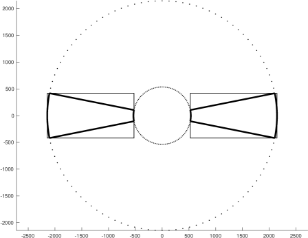
Figure 1: The support of $\widehat{\gamma_{j,0,0}}$ for $j=8$ (with thick boundary), contained in $I_{j}$.

An exercise in planar geometry shows that for $j\geq 2$, ${\rm supp}\,\chi_{j}$ is contained in the union of disjoint rectangles

$$I_{j}:=\left(\left[-\frac{8\pi}{3}2^{j},-t_{j}\right]\times\left[-\frac{\lambda_{j}}{2},\frac{\lambda_{j}}{2}\right]\right)\cup\left(\left[t_{j},\frac{8\pi}{3}2^{j}\right]\times\left[-\frac{\lambda_{j}}{2},\frac{\lambda_{j}}{2}\right]\right)$$

where $\frac{\lambda_{j}}{2}:=2^{j}\frac{8\pi}{3}\sin(2^{-\lfloor j/2\rfloor}{\pi})$ and $t_{j}:=2^{j}\frac{2\pi}{3}\cos(2^{-\lfloor j/2\rfloor}{\pi})$. Furthermore, we set $\Lambda_{j}:=2(\frac{8\pi}{3}2^{j}-t_{j})$, so that $t_{j}+\frac{\Lambda_{j}}{2}:=\frac{8\pi}{3}2^{j}$ (this is illustrated in Figure 1 below). It follows that $\lambda_{j}$ is the total height of the support of $\chi_{j}$ and $\Lambda_{j}$ is the total width. Also, $\chi_{0}$ is supported on the square $[-\frac{8\pi}{3},\frac{8\pi}{3}]^{2}$, and $\chi_{1}$ is supported on $[-\frac{16\pi}{3},\frac{16\pi}{3}]^{2}$. For notational convenience, we define $\Lambda_{0}:=\lambda_{0}:=\frac{16\pi}{3}$ and $\Lambda_{1}:=\lambda_{1}:=\frac{32\pi}{3}$.

The $j$-dependent grids are then defined as $\mathbb{X}_{j}:=\{\left(\frac{k_{1}}{\Lambda_{j}},\frac{k_{2}}{\lambda_{j}}\right)\mid k\in 2\pi\mathbb{Z}^{2}\}$.

Remark 17.

For $j\in\mathbb{N}$, define $\varepsilon_{1}(j):=\Lambda_{j}2^{-j}$ and $\varepsilon_{2}(j):=\lambda_{j}{2^{-\lfloor j/2\rfloor}}$. Define the grid correction matrix $D_{\varepsilon}^{(j)}$ as $D_{\varepsilon}^{(j)}:=\begin{pmatrix}\varepsilon_{1}(j)&0\\ 0&\varepsilon_{2}(j)\end{pmatrix}$. Then $\begin{pmatrix}\Lambda_{j}&0\\ 0&\lambda_{j}\end{pmatrix}=D_{j}D_{\varepsilon}^{(j)}$, and we have

$$\mathbb{X}_{j}=2\pi(D_{\varepsilon}^{(j)})^{-1}D_{j}^{-1}\mathbb{Z}^{2}.$$

Note that, for $j\geq 2$, $\varepsilon_{1}(j)=\frac{4\pi}{3}[4-\cos(2^{-\lfloor j/2\rfloor}{\pi})]$, and $\varepsilon_{2}(j)={2^{-\lfloor j/2\rfloor}}[\frac{16\pi}{3}2^{j}\sin(2^{-\lfloor j/2\rfloor}\pi)]$. This implies, indeed, that $\varepsilon_{\ell}$, $\ell=1,2$, are uniformly bounded from above and away from $0$: The estimates

$$\begin{array}[]{lclc}4\pi&\leq\varepsilon_{1}(j)&\leq\frac{16\pi}{3},\\ \frac{32\pi}{3}&\leq\varepsilon_{2}(j)&\leq\frac{32\pi^{2}}{3}.\end{array}$$ (33)

hold.

Curvelets

The curvelet $\gamma$ with $\mu(\gamma)=(j,\ell,k)$, with $j\in\mathbb{N}$, $\ell\in\mathbb{N}\cap[0,2^{\lfloor j/2\rfloor}-1]$ and $k\in\mathbb{X}_{j}$, is defined as

$$\gamma:=\gamma_{j,\ell,{k}}(x):=\frac{1}{\sqrt{\Lambda_{j}\lambda_{j}}}(\mathcal{F}^{-1}\chi_{j})(R_{j,\ell}^{*}x-{k}).$$

Note that if $j=0$, then $\ell=0$. If we set $\bm{\gamma}^{(j)}:=|D_{j}|^{-1/2}\gamma_{j,0,{0}}(D_{-j}\cdot)$, then equation (2), namely $\gamma_{j,\ell,{k}}=|D_{j}|^{1/2}\bm{\gamma}^{(j)}(D_{j}(R_{j,\ell}^{*}\cdot-k))$, follows automatically. Indeed, we have

$$\widehat{\bm{\gamma}^{(j)}}(\xi)=|D_{j}|^{1/2}\widehat{\gamma_{j,0,0}}(D_{j}\xi)=\sqrt{\frac{|D_{j}|}{\Lambda_{j}\lambda_{j}}}\chi_{j}(D_{j}\xi).$$ (34)

At this point, we define

$$\mathcal{D}_{curv}:=\{\gamma_{0,0,k}\mid k\in\mathbb{X}_{0}\}\cup\{\gamma_{1,0,k}\mid k\in\mathbb{X}_{1}\}\cup\left\{\gamma_{j,\ell,k}\mid j\geq 2,\ell\in\{0,\dots,2^{\lfloor j/2\rfloor}-1\},k\in\mathbb{X}_{j}\right\}.$$

From this we have the following two results.

Lemma 18.

Let $A:=\frac{\sqrt{2}\pi}{3}$ and $B:=\frac{16\pi^{2}}{3}$. For all $j$, $\mathrm{supp}(\widehat{\bm{\gamma}^{(j)}})\subset[-B,B]^{2}$. For $j\geq 4$, $\widehat{\bm{\gamma}^{(j)}}(\xi)=0$ when $|\xi|\leq A$.

Proof.

This follows from (34); namely, the fact that $\mathrm{supp}(\widehat{\bm{\gamma}^{(j)}})=D_{-j}\,\mathrm{supp}(\chi_{j})$, which, together with some of the construction details before, gives $B=\max_{j}2^{-\lfloor j/2\rfloor}\frac{\lambda_{j}}{2}$ and $A=\min_{j\geq 4}2^{-j}t_{j}$. ∎

Lemma 19.

For each multi-index $\alpha=(\alpha_{1},\alpha_{2})$, there is $C_{\alpha}$ so that for all $j\geq 4$

$$\|D^{\alpha}\widehat{\bm{\gamma}^{(j)}}\|_{\infty}\leq C_{\alpha}.$$

Proof.

By (34), it suffices to consider $\chi_{j}(D_{j}\cdot)$ in place of $\bm{\gamma}^{(j)}$, since $\sqrt{\frac{|D_{j}|}{\Lambda_{j}\lambda_{j}}}=\sqrt{\varepsilon_{1}(j)\varepsilon_{2}(j)}$ is bounded above and below by Remark 17. We have that

$$\chi_{j}(D_{j}\xi)=w\left(\sqrt{\xi_{1}^{2}+(2^{-\lceil j/2\rceil}\xi_{2})^{2}})\right)v\bigl{(}2^{\lfloor j/2\rfloor}\tan^{-1}\bigl{(}2^{-\lceil j/2\rceil}{\xi_{2}}/{\xi_{1}}\bigr{)}\bigr{)}.$$

The result follows from the smoothness of the functions involved, and the fact that $|\xi_{1}|,|\xi_{2}|\leq B$ and $|\xi_{1}|>A>0$. ∎

References

• [1] Fabio Aiolli and Michele Donini. Learning anisotropic RBF kernels. In International Conference on Artificial Neural Networks, pages 515โ€“522. Springer, 2014.
• [2] Fredrik Andersson, Marcus Carlsson, and Luis Tenorio. On the representation of functions with Gaussian wave packets. J. Fourier Anal. Appl., 18(1):146โ€“181, 2012.
• [3] Ted Belytschko, Timon Rabczuk, Antonio Huerta, and Sonia Fernรกndez-Mรฉndez. Meshfree methods. In Encyclopedia of Computational Mechanics. John Wiley & Sons, Ltd, 2004.
• [4] Jeffย A Bilmes. A gentle tutorial of the EM algorithm and its application to parameter estimation for Gaussian mixture and hidden Markov models. Technical Report ICSI-TR-97-021, International Computer Science Institute, Berkeley, CA, 1998.
• [5] Emmanuelย J. Candรจs and Davidย L. Donoho. New tight frames of curvelets and optimal representations of objects with piecewise $C^{2}$ singularities. Comm. Pure Appl. Math., 57(2):219โ€“266, 2004.
• [6] Olivier Chapelle, Vladimir Vapnik, Olivier Bousquet, and Sayan Mukherjee. Choosing multiple parameters for support vector machines. Machine learning, 46(1):131โ€“159, 2002.
• [7] Gong Cheng and Victor Shcherbakov. Anisotropic radial basis function methods for continental size ice sheet simulations. Journal of Computational Physics, 372(1):161โ€“177, 2018.
• [8] Ole Christensen and Asghar Rahimi. Frame properties of wave packet systems in $L^{2}(\mathbb{R}^{d})$. Adv. Comput. Math., 29(2):101โ€“111, 2008.
• [9] Maartenย V. deย Hoop, Karlheinz Grรถchenig, and Josรฉย Luis Romero. Exact and approximate expansions with pure Gaussian wave packets. SIAM J. Math. Anal., 46(3):2229โ€“2253, 2014.
• [10] Ronald DeVore and Amos Ron. Approximation using scattered shifts of a multivariate function. Trans. Amer. Math. Soc., 362(12):6205โ€“6229, 2010.
• [11] Huongย Quynh Dinh, Greg Turk, and Greg Slabaugh. Reconstructing surfaces using anisotropic basis functions. In Computer Vision, 2001. ICCV 2001. Proceedings. Eighth IEEE International Conference on, volumeย 2, pages 606โ€“613. IEEE, 2001.
• [12] Leslie Greengard and June-Yub Lee. Accelerating the nonuniform fast Fourier transform. SIAM review, 46(3):443โ€“454, 2004.
• [13] Michael Griebel and Jan Hamaekers. Tensor product multiscale many-particle spaces with finite-order weights for the electronic Schrรถdinger equation. Zeitschrift fรผr Physikalische Chemie, 224(3-4):527โ€“543, 2010.
• [14] Philipp Grohs and Gitta Kutyniok. Parabolic molecules. Found. Comput. Math., 14(2):299โ€“337, 2014.
• [15] Thomas Hangelbroek and Amos Ron. Nonlinear approximation using Gaussian kernels. J. Funct. Anal., 259(1):203โ€“219, 2010.
• [16] Thomas Kรผhn. Covering numbers of Gaussian reproducing kernel Hilbert spaces. J. Complexity, 27(5):489โ€“499, 2011.
• [17] G.ย Kyriazis and P.ย Petrushev. New bases for Triebel-Lizorkin and Besov spaces. Trans. Amer. Math. Soc., 354(2):749โ€“776, 2002.
• [18] Demetrio Labate, Guido Weiss, and Edward Wilson. An approach to the study of wave packet systems. In Wavelets, frames and operator theory, volume 345 of Contemp. Math., pages 215โ€“235. Amer. Math. Soc., Providence, RI, 2004.
• [19] Wingย Kam Liu, Yijung Chen, R.ย Aziz Uras, and Chinย Tang Chang. Generalized multiple scale reproducing kernel particle methods. Comput. Methods Appl. Mech. Engrg., 139(1-4):91โ€“157, 1996.
• [20] Sergei Manzhos, Xiaogang Wang, and Tucker Carringtonย Jr. A multimode-like scheme for selecting the centers of Gaussian basis functions when computing vibrational spectra. Chemical Physics, 509:139โ€“144, 2017.
• [21] Vladimir Mazโ€™ya and Gunther Schmidt. Approximate approximations, volume 141 of Mathematical Surveys and Monographs. American Mathematical Society, Providence, RI, 2007.
• [22] Yves Meyer. Wavelets and operators, volumeย 37 of Cambridge Studies in Advanced Mathematics. Cambridge University Press, Cambridge, 1992. Translated from the 1990 French original by D. H. Salinger.
• [23] Partha Niyogi and Federico Girosi. Generalization bounds for function approximation from scattered noisy data. Advances in Computational Mathematics, 10(1):51โ€“80, Jan 1999.
• [24] Carlย Edward Rasmussen. The infinite Gaussian mixture model. In Advances in neural information processing systems 12, pages 554โ€“560, 2000.
• [25] Amos Ron and Zuowei Shen. Generalized shift-invariant systems. Constr. Approx., 22(1):1โ€“45, 2005.
• [26] Ingo Steinwart and Clint Scovel. Fast rates for support vector machines using Gaussian kernels. Ann. Statist., 35(2):575โ€“607, 2007.
• [27] Holger Wendland. Scattered data approximation, volumeย 17 of Cambridge Monographs on Applied and Computational Mathematics. Cambridge University Press, Cambridge, 2005.
• [28] Lei Xu and Michaelย I Jordan. On convergence properties of the EM algorithm for Gaussian mixtures. Neural computation, 8(1):129โ€“151, 1996.
• [29] Yiming Ying and Ding-Xuan Zhou. Learnability of Gaussians with flexible variances. J. Mach. Learn. Res., 8:249โ€“276 (electronic), 2007.