A dynamical Toric Code model with fusion and de-fusion

Abstract

We introduce a two-parameter family of perturbations of Kitaev’s Toric Code Model in which the anyonic excitations acquire an interesting dynamics. We study the dynamics of this model in the space of states with electric and magnetic charge both equal to 1 and find that the model exhibits both bound states and scattering states in a suitable region of the parameters. The bound state is a Majorana fermion with a dispersion relation of Dirac cone type. For a certain range of model parameters, we find that these bound states disappear in a continuum of scattering states at a critical value of the total momentum. The scattering states describe separate electric and magnetic anyons, which in this model each have a $\sin k$ dispersion relation.

I Introduction

There is increasing evidence that Majorana fermions and various types of anyons occur in the quantum many-body systems that exhibit topological order willett:2013 ; morampudi:2017 ; knapp:2019 ; takane:2019 . Toy models such as Kitaev’s quantum double models kitaev:2003 and the Levin-Wen string-net models levin:2005 have been instrumental in showing that short-range lattice Hamiltonians in two dimensions can exhibit a rich variety of anyonic excitation spectra. Another important step was achieved by Bravyi, Hastings, and Michalakis bravyi:2010 and, independently, Klich klich:2010 , when they showed that the spectral gap above the ground state of these models is stable against sufficiently weak but otherwise arbitrary perturbations. In cha:2018a it was shown that not only the gap, but the specific structure of anyon types and the associated superselection sectors too are stable in the same sense.

One of the virtues of the Toric Code Model (TCM) is that it is explicitly solvable and the structure of its eigenstates can be given explicitly and fully understood. This is possible because it is a so-called ‘commuting Hamiltonian’, meaning that all terms in the Hamiltonian (2) commute and, hence, can be simultaneously diagonalized. It shares this property with the entire class of quantum double models introduced by Kitaev kitaev:2003 and many other models as well. The commuting property has a drawback, however, since it implies that the model has no meaningful dynamics. The particle-like excitations, the anyons, are dispersionless (flat bands), and are therefore static. To explore the properties of anyons in a more realistic setting, we set out to modify the TCM by adding new finite-range interactions to Kitaev’s Hamiltonian while at the same time aiming to preserve as many of its symmetries as possible. First and foremost, we want to preserve the anyon structure of the model. Equivalently, we want to preserve the superselection sectors, which are labeled by the charges corresponding to the quantum-double $\mathbb{Z}_{2}\times\mathbb{Z}_{2}$. We will label the four superselection sectors by $0$ (the vacuum sector), $\epsilon$ (odd electric and even magnetic charge), $\mu$ (even electric and odd magnetic charge), and $\epsilon\mu$ (electric and magnetic charges both odd). The TCM does not only preserve the topological charge, given by the parities of the electric and magnetic charge but, via the energy, in fact preserves the integer values of both types of charges (particle number conservation). By respecting these conservation laws we will guarantee that the vacuum state itself is left invariant under the perturbations we consider and it also implies the existence of an invariant subspace of states with one electric and one magnetic anyon present. In this paper, our primary interest is the spectrum of the Dynamical Toric Code Model (DTCM) that we introduce below, in that subspace.

II The space of states with unit topological charge

Kitaev’s TCM is a two-dimensional quantum spin model that is commonly defined on the regular square lattice $\mathbb{Z}^{2}$. It has a duality symmetry that is most directly seen if we use the edges of the square lattice to label the spins. Let $\mathcal{V}$, $\mathcal{E}$, $\mathcal{F}$, denote the set of vertices, the set of edges, and the set of faces, respectively, of the regular square lattice. For each $v\in\mathcal{V}$ and $f\in\mathcal{F}$, define

$$A_{v}=\prod_{e,v\in e}\sigma^{1}_{e},\quad B_{f}\prod_{e,e\in f}\sigma^{3}_{e}.$$ (1)

These are often referred to as the star and plaquette operators of the toric code. In terms of these, the TCM is defined by the Hamiltonian

$$H^{TC}=\sum_{v\in\mathcal{V}}(\mathbb{1}-A_{v})+\sum_{f\in\mathcal{F}}(\mathbb{1}-B_{f}).$$ (2)

For our purposes, the infinite lattice setting is best suited. First, the difference between bound states and scattering states is a clear mathematical distinction for the infinite system. Second, there are well-defined sectors of the model with single anyon excitations, while in finite volume such excitations are always created in pairs starting from the vacuum. By considering the infinite lattice, we can consider the limit where one of the anyons of a pair is taken to infinity. This leads to a simple structure of superselection sectors naaijkens:2011 ; cha:2018 which has recently been shown to be stable under perturbations of the Hamiltonian cha:2018a . Let us recall the main features of the TCM on the infinite lattice in some detail.

As shown in alicki:2007 , the TCM on infinite lattice $\mathbb{Z}^{2}$ has a unique frustration free ground state, meaning there is a unique state fully determined by the vanishing of all terms in the Hamiltonian:

$$\omega(\mathbb{1}-A_{v})=\omega(\mathbb{1}-B_{f})=0,\mbox{ for all }v\in\mathcal{V},f\in\mathcal{F}.$$

Here, the state is represented by its expectation functional $\omega$. It will be useful to use a representation of this state as a unit vector $\Omega$ in the vacuum Hilbert space $\mathcal{H}_{0}$:

$$\omega(A)=\langle\Omega,\pi(A)\Omega\rangle,$$ (3)

where $A$ is an arbitrary observable involving a finite set of spins, and $\pi$ is a representation of the observables acting on the Hilbert space $\mathcal{H}_{0}$. $\mathcal{H}_{0}$ itself represents all excitations of the model that can be created by such an observable acting on the vacuum state. This includes pairs of excitations created by finite string operators (see below). The representation (3) is known as the Gelfand-Naimark-Segal (GNS) representation of the vacuum state bratteli:1987 . The vacuum vector $\Omega$ is characterized by the property that it is an eigenvector with eigenvalue 1 of each of the operators $A_{v}$ and $B_{f}$:

$$\pi(A_{v})\Omega=\pi(B_{f})\Omega=\Omega,\quad v\in\mathcal{V},f\in\mathcal{F}.$$

Energy eigenstates in the vacuum sector are created by the action of the so-called string operators. These are associated with paths over edges of either the lattice or the dual lattice as follows. Let $\gamma$ and $\tilde{\gamma}$ be a finite path in the lattice and the dual lattice, respectively, and define

$$F^{\epsilon}_{\gamma}=\prod_{e\in\gamma}\sigma^{3}_{e},\quad F^{\mu}_{\tilde{\gamma}}=\prod_{e\in\tilde{\gamma}}\sigma^{1}_{e}.$$

Here, we have used the fact that the edges of the lattice and the edges of the dual lattice are in one-to-one correspondence. Hence, we can use the same notation for them. Moreover, each spin is associated with exactly one edge of the lattice and one edge of the dual lattice. Using the commutation relations of the Pauli matrices (which are preserved by any representation $\pi$), it is straightforward to check that the vectors

$$\pi(F^{\epsilon}_{\gamma})\Omega,\mbox{ and }\pi(F^{\mu}_{\tilde{\gamma}})\Omega$$

are eigenstates of the Hamiltonian and that these vectors only depend on the end-points of the paths. In particular, closed paths leave $\Omega$ invariant, and each string operator corresponding to a finite open path generates an eigenstate with energy $4$, corresponding to an eigenvalue $-1$ for the two terms $A_{v}$ and $A_{v^{\prime}}$ where $v$ and $v^{\prime}$ are the end points of the path $\gamma$ or $B_{f}$ and $B_{f^{\prime}}$, with $f$ and $f^{\prime}$ the two end faces of the dual path $\tilde{\gamma}$. Due to the invariance of $\Omega$ under closed string operators, which is an expression of the gauge invariance of the model, the eigenstates created by a single open string operator are consistently defined, including their phase. This changes when we consider the states created by the combined action of a string operator and a dual string operator. The two anti-commute when the strings intersect an odd number of times and commute otherwise. The vectors created from the vacuum by the action of both a string operator and a dual string operator on $\Omega$ may therefore differ by a minus sign depending on the choice of paths connecting a given pair of end points. This does not affect expectation values of any observable in the excited states, but is relevant when calculating matrix elements of operators relating different excited states.

The expectation functionals for excited states with just one anyon, of which energy equals 2, can be defined unambiguously by considering a sequence of paths with one end point held fixed while the other end point is taken to infinity. In such a limit, the expectation value of any observable depends only on the location of the end point that is held fixed. This is easily verified using the invariance of the vacuum under the action of closed-string operators.

It will be convenient to express the single anyon states as a modified representation of the algebra of observables. Note that the operators $F^{\epsilon}_{\gamma}$ and $F^{\mu}_{\tilde{\gamma}}$ are self-adjoint unitaries that square to $\mathbb{1}$. Therefore, conjugation with these operators defines a family of automorphisms of the algebra of observables. In order to set up a convention for a Hilbert space of excitations as vectors states, we now fix a convention for how the endpoints of the paths are taken to infinity. We introduce families of paths $\gamma_{v}(n)$ and $\tilde{\gamma}_{f}(n)$ which start at a vertex $v$ and face $f$, respectively, and stretch over $n$ edges and dual edges in the negative vertical direction, from $v$ to $v-n\hat{y}$ and similarly for $f$ in the dual lattice. We can now define the following automorphisms of the observable algebra as limits along these paths:

$$\alpha_{v}(A) = \lim_{n\to\infty}F^{\epsilon}_{\gamma_{v}(n)}AF^{\epsilon}_{\gamma_{v}(n)}$$ (4)

$$\alpha_{f}(A) = \lim_{n\to\infty}F^{\mu}_{\tilde{\gamma}_{f}(n)}AF^{\mu}_{\tilde{\gamma}_{f}(n)}$$ (5)

It is easy to see that all these automorphisms commute and that the families $\{\alpha_{v}\mid v\in\mathcal{V}\}$ and $\{\alpha_{f}\mid f\in\mathcal{F}\}$ are covariant with respect to the automorphisms representing lattice translations: for all $x\in\mathbb{Z}^{2}$ one has

$$T_{x}\circ\alpha_{v} = \alpha_{v+x}\circ T_{x}$$

$$T_{x}\circ\alpha_{f} = \alpha_{f+x}\circ T_{x},$$

where $v+x$ and $f+x$ denote the translated vertex and face in the lattice. We are interested in the family of states

$$A\mapsto\omega_{v,f}(A):=\langle\Omega,\pi\circ\alpha_{v}\circ\alpha_{f}(A)\Omega\rangle.$$

It is easy to see that the representations $\pi\circ\alpha_{v}\circ\alpha_{f}$ are all unitarily equivalent. Therefore, the states $\omega_{v,f}$ can all be represented as vector states in one and the same Hilbert space. This Hilbert space, however, is distinct from the one that contains the vacuum vector. It is an in-equivalent superselection sector, corresponding to different values of the topological charges.

Furthermore, if $(v,f)\neq(v^{\prime},f^{\prime})$, there is $X\in\{A_{v},B_{f}\}$ such that the expectations $\omega_{v,f}(X)$ $\omega_{v^{\prime},f^{\prime}}(X)$ are given by distinct eigenvalues of $X$. This implies that the vector states are mutually orthogonal. As a result, there is a natural identification of the states with a single electric and magnetic excitation with $\ell^{2}(\mathcal{V}\times\mathcal{F})\cong\operatorname{span}\{\psi(v,f)|v\in\mathcal{V},f\in\mathcal{F}\}=:\mathcal{H}^{\epsilon\mu}$ on which the translations act by unitaries $U_{x},x\in\mathbb{Z}^{2}$, in the canonical way.

Note that we can reason in exactly the same way to construct Hilbert spaces $\mathcal{H}^{\epsilon}$ and $\mathcal{H}^{\mu}$ of states with a single electric and magnetic excitation, respectively. Each of the three Hilbert spaces $\mathcal{H}^{\epsilon},\mathcal{H}^{\mu}$, and $\mathcal{H}^{\epsilon\mu}$ belong to its own superselection sector distinct from one another and from the vacuum sector naaijkens:2011 . We will use these spaces to motivate the perturbation terms we introduce to define the Dynamical Toric Code Model (DTCM) in the next section. We have that $\mathcal{H}^{\epsilon}\cong\ell^{2}(\mathcal{V})$, $\mathcal{H}^{\mu}\cong\ell^{2}(\mathcal{F})$, and $\mathcal{H}^{\epsilon\mu}\cong\ell^{2}(\mathcal{V}\times\mathcal{F})$. We will use the natural orthonormal bases of anyon excitations $\{\ket{\epsilon_{v}}\}_{v\in\mathcal{V}}$, $\{\ket{\mu_{f}}\}_{f\in\mathcal{F}}$, and $\{\ket{\epsilon_{v},\mu_{f}}\}_{v\in\mathcal{V},f\in\mathcal{F}}$ for these spaces.

III A Dynamical Toric Code model

Since the static anyon excitations $\ket{\epsilon_{v}}$ and $\ket{\mu_{f}}$, loosely speaking, correspond to the action of a half-infinite string operator starting at $v$ and $f$, hopping terms that move the excitation should move the end point of the corresponding string operator. This amounts to the action of a Pauli matrix at a neighboring spin (extending the path) or at the end point itself, which shrinks the path by one unit. The action of the Pauli matrices by themselves at a generic location, however, would create a pair of additional excitations and create a state of energy equal to $6$ and orthogonal to the space of single anyon excitations. In order to achieve our goal of leaving the spaces $\mathcal{H}^{\epsilon}$ and $\mathcal{H}^{\mu}$ invariant under the action of the hopping terms, we use the operators $A_{v}$ and $B_{f}$ to detect the location of the excitation. It turns out that hopping matrix elements are imaginary and have the correct sign with respect to a reference orientation, which by the gauge symmetry one can freely chose. There is complex, non translation-invariant gauge transformation that makes the hopping matrix elements real, but working in that gauge would not offer any advantages. A simple translation-invariant orientation is the following: let all horizontal edges point to the right and all vertical edges point up. In terms of this orientation we define a sign function on the pairs $(v,e)\in\mathcal{V}\times\mathcal{E},v\in e$ as follows: Define $s(v,e)=1$, if $e$ is outgoing with respect to $v$, and $s(v,e)=-1$, if $e$ is incoming with respect to $v$. The sign of a face $f$ with respect to an edge $e$, denoted by $s(f,e)$ is defined consistent with the duality of faces to vertices: $s(f,e)=1$ if $f$ is below or to the left of $e$ and $s(f,e)=-1$ if $f$ is above or to the right of $e$.

The hopping terms that satisfy our criteria are then

$$H^{\epsilon}:=i\sum_{e}\sigma^{3}_{e}\sum_{v\in e}s(v,e)A_{v}.$$ (6)

and

$$H^{\mu}:=i\sum_{e}\sigma^{1}_{e}\sum_{f\ni e}s(f,e)B_{f}$$ (7)

To find the spectrum, we first find the matrix elements of $H^{\epsilon}$ and $H^{\mu}$, restricted to the invariant subspaces $\mathcal{H}^{\epsilon}$ and $\mathcal{H}^{\mu}$, with respect to the orthonormal bases $\{\ket{\epsilon_{v}}\}_{v\in\mathcal{V}}$ and $\{\ket{\mu_{f}}\}_{f\in\mathcal{F}}$, respectively. To do this, we identify the vertex set $\mathcal{V}$ with a copy of the integer lattice $\mathbb{Z}^{2}$ and define $S$ to be the set of unit lattice vectors: $S=\{\hat{x},-\hat{x},\hat{y},-\hat{y}\}$. Then, the matrix elements of $H^{\epsilon}$ restricted to $\mathcal{H}^{\epsilon}$ are given by

$$\bra{\epsilon_{v^{\prime}}}H^{\epsilon}\ket{\epsilon_{v}}=2i\sum_{r\in S}(r\cdot\hat{x}+r\cdot\hat{y})\delta_{v^{\prime},v+r}$$ (8)

The spectrum and the dispersion relation are then easily found by Fourier transformation:

$$E(k)=4\sin(k_{x})+4\sin(k_{y}),k_{x},k_{y}\in[0,2\pi).$$ (9)

The magnetic anyons described by $H^{\mu}$ have the same spectrum.

Since we are interested in seeing the dynamical properties of interacting anyons and specifically the merging of an electric and a magnetic excitation into an excitation created by what is called a ribbon operator bombin:2008 , we also need to consider adding terms to the Hamiltonian that describe electric-magnetic interactions. Formally, we again have an orthonormal basis of $\mathcal{H}^{\epsilon\mu}$ with one electric anyon at the vertex $v$ and one magnetic anyon at the face $f$ created by a pair of string operators, with the same convention of paths and dual paths extending to $\infty$ in the negative $\hat{y}$ direction:

$$\ket{\epsilon_{v}\mu_{f}}=F^{\epsilon}_{\gamma_{v}}F^{\mu}_{\tilde{\gamma}_{f}}\ket{\Omega}.$$ (10)

If $v$ and $f$ are such that there is an edge $e$ satisfying $v\in e$, $e\in f$ ($v$ and $f$ are next to each other) then this represents a fused $\epsilon\mu$ state that we denote by $\ket{\epsilon\mu_{s}}$, where $s$ is a ‘site’ determined by a pair $(v,f)$, where $v$ is a vertex belonging to the face $f$. The ribbon states correspond to the pairs $(v,f)$ with $v\in f$. Using the same principles as for the single $\epsilon$ and $\mu$ hopping terms we constructed a hopping term that leaves the subspace of ribbon states invariant:

$$H^{\epsilon\mu}= i\sum_{e}\sigma^{3}_{e}\sum_{v\in e}s(v,e)A_{v}\sum_{f\ni e}(\mathbb{1}-B_{f})$$ (11)

$$+ i\sum_{e}\sigma^{1}_{e}\sum_{f\ni e}s(f,e)B_{f}\sum_{v\in e}(\mathbb{1}-A_{v}).$$ (12)

Note that, individually, the terms $H^{\epsilon},H^{\mu}$, and $H^{\epsilon\mu}$ leave the sectors with one $\epsilon$, one $\mu$, and one $\epsilon$ plus one $\mu$ excitation invariant. Ribbon states, however, may be broken up by $H^{\epsilon}$ and $H^{\mu}$. Using these three terms we define the Hamiltonian of the Dynamical Toric Code model (DTCM) as follows:

$$H^{\rm DTC}=H^{\rm TC}+\lambda_{\epsilon}H^{\epsilon}+\lambda_{\mu}H^{\mu}+\rho H^{\epsilon\mu}.$$ (13)

IV Symmetries

Before analyzing the DTCM, let us observe important symmetries of $H^{\rm TC}$ and $H^{\rm DTC}$. In addition to the translation and 4-fold rotation symmetry of the lattice, the TCM also has lattice inversion (aka parity), time reversal, spin-flip, charge conjugation, chirality, and duality symmetries, which we now discuss.

Lattice inversion or parity symmetry stems from the lattice invariance under reflection through the origin: $(x_{1},x_{2})\to(-x_{1},-x_{2})$. The terms appearing in the perturbations $H^{\epsilon},H^{\mu}$, and $H^{\epsilon\mu}$ all anti-commute with inversion due to the presence of the signs $s(v,e)$ and $s(f,e)$. The vacuum state is invariant under parity. Therefore the symmetry is represented by a unitary operator $P$ in the GNS representation (as is also the case in finite volume, of course).

Since $P$ commutes with $H^{\rm TC}$ but anti-commutes with the perturbation terms in $H^{\rm DTC}$, the perturbed spectrum in the single anyon sectors is symmetric around the unperturbed excitation energy, as is illustrated in Figure 3.

Time reversal, an anti-unitary $T$ with $T^{2}=\mathbb{1}$, implemented by complex conjugation combined either spin flip ($T\sigma^{i}=-\sigma^{i}T,i=1,2,3$) or parity. We have $[H^{\rm DTC},T]=0$. This has an important implication for the spectrum of $H^{\epsilon\mu}$ restricted to $\mathcal{H}^{\epsilon\mu}$, as the $\epsilon\mu$ particle has fermion self-statistics. This means in this sector that Kramer’s degeneracy implies an even degeneracy for all values of the spectrum.

Charge conjugation is an anti-unitary $C$ with $C^{2}=\mathbb{1}$, implemented by complex conjugation by itself. We have $\{H^{\rm DTC}-H^{\rm TC},C\}=0$ and $[H^{\rm TC},C]=0$.

Chirality is described by a unitary $S$ with $S^{2}=\mathbb{1}$, implemented by either spin flip or parity. We have $\{H^{\rm DTC}-H^{\rm TC},S\}=0$ and $[H^{\rm TC},S]=0$.

The $\mathbb{Z}_{2}\times\mathbb{Z}_{2}$ symmetry given by the spin rotations by $\pi$ are implemented by the conjugation with the Pauli matrices. These ‘spin flip’ symmetries are broken in $H^{\rm DTC}$.

Duality symmetry, which interchanges the lattice and the dual lattice, is implemented by a local unitary operator taking the form

$$D=\frac{1}{\sqrt{2}}\left(\begin{matrix}1&1\\ 1&-1\end{matrix}\right)$$ (14)

D has the following properties

$$D^{2} =\mathbb{1}$$ (15)

$$D\sigma^{1}D =\sigma^{3}$$ (16)

$$D\sigma^{3}D =\sigma^{1}$$ (17)

$$D\sigma^{2}D =-\sigma^{2}$$ (18)

Duality interchanges $\epsilon$ and $\mu$ excitations:

$$[D,H^{\rm TC}] =[D,H^{\epsilon\mu}]=0$$ (19)

$$DH^{\epsilon}D =H^{\mu}$$ (20)

Therefore, if $\lambda_{\mu}=\lambda_{\epsilon}:=\lambda$, we have that $[D,H^{\rm DTC}]=0$.

V The Hamiltonian in the $\epsilon\mu$ sector

As mentioned above, the Hilbert space of single-anyon excitations in the $\epsilon,\mu$ and $\epsilon\mu$ sector are individually left invariant. Therefore, the dispersion relation for each anyon type is well-defined and is easily computed as long as one takes care to define a suitable basis in the appropriate Hilbert space. The Hilbert space of states with exactly one electric and one magnetic anyon, $\mathcal{H}^{\epsilon\mu}$, is a subspace of the $\epsilon\mu$ sector and is invariant for the Hamiltonian $H^{DTCM}$ defined in (13). To calculate its spectrum we will find its matrix elements with respect to the basis $\{\ket{\epsilon_{v}\mu_{f}}\}_{v\in\mathcal{V},f\in\mathcal{F}}$.

Since the vacuum state is also the ground state of the DTCM, at least for $\lambda$ and $\rho$ not too large bravyi:2010 (and generally is a stationary state), the dynamics of the states $\ket{\epsilon_{v}\mu_{f}}$ can be studied in terms of commutation properties of the Hamiltonian with the operators $F^{\epsilon}_{\gamma_{v}(n)}$ and $F^{\mu}_{\tilde{\gamma}_{f}(n)}$ and the property that the vacuum state is invariant under closed loop operators. It follows that we can analyze the dynamics of the states $\ket{\epsilon_{v}\mu_{f}}$ in terms of a Hamiltonian $h^{\epsilon\mu}$ on $\ell^{2}(\mathcal{V}\times\mathcal{F})$, which is unitarily equivalent to the invariant subspace $\mathcal{H}^{\epsilon\mu}$. All we need to do is calculate the matrix of $H^{DTCM}$ with respect to the basis states $\ket{\epsilon_{v}\mu_{f}}$.

The term $H^{TC}$ acts as a constant (=4) on the subspace $\mathcal{H}^{\epsilon\mu}$. The dynamics of the DTCM restricted to $\mathcal{H}^{\epsilon\mu}$ is therefore solely due to the terms $H^{\epsilon},H^{\mu}$, and $H^{\epsilon\mu}$. It is also clear from its definition that $h^{\epsilon\mu}$ commutes with the lattice translations acting on $\mathcal{H}^{\epsilon\mu}$. After taking the Fourier transform with respect to the ‘center of mass’ coordinates $X$, and writing $(v,f)=(X-d,X+d)$, we obtain a useful expression for $h^{\epsilon\mu}$ on the subspace of total quasi-momentum $K$. It is convenient to consider the even and odd square sublattices of $\mathbb{Z}^{2}$ to label the vertices $\mathcal{V}$ and the faces $\mathcal{F}$, respectively. This implies that the relative coordinates $d$ are to be taken in $(2\mathbb{Z}+1)^{2}$. We will use the notation $d=d_{1}\hat{x}+d_{2}\hat{y}$, where $\hat{x}=(1,0),\hat{y}=(0,1)$. We also define the function $\theta$ on the odd integers by $\theta(d)=(1-\operatorname{sign}(d))/2$.

A careful calculation yields the following matrix elements of $h$ in the subspace of states with total quasi-momentum $K=(K_{1},K_{2})$: for $d^{\prime},d\in(2\mathbb{Z}+1)^{2}$ we have

$$(h_{K})_{d^{\prime},d} = -2\lambda H^{0}_{d^{\prime},d}(K)-2\rho H^{i}_{d^{\prime},d}(K)$$

$$(H^{0}_{K})_{d^{\prime},d} = \sin 2K_{1}[\delta_{d^{\prime},d-2\hat{x}}(-1+2\delta_{d_{1},1}\theta(d_{2}))$$

$$+\delta_{d^{\prime},d+2\hat{x}}(-1+2\delta_{d_{1},-1}\theta(d_{2}))]$$

$$-\sin 2K_{2}[\delta_{d^{\prime},d-2\hat{y}}+\delta_{d^{\prime},d+2\hat{y}}]$$

$$(H^{i}_{K})_{d^{\prime},d} = \sin 2K_{1}[\delta_{d^{\prime},d-2\hat{x}}\delta_{d_{1},1}(\delta_{d_{2},1}-\delta_{d_{2},-1})$$

$$+\delta_{d^{\prime},d+2\hat{x}}\delta_{d_{1},-1}(\delta_{d_{2},1}-\delta_{d_{2},-1})]$$

$$-\sin 2K_{2}[\delta_{d^{\prime},d-2\hat{y}}\delta_{d_{2},1}(\delta_{d_{1},1}+\delta_{d_{1},-1})$$

$$+\delta_{d^{\prime},d+2\hat{y}}\delta_{d_{2},-1}(\delta_{d_{1},1}+\delta_{d_{1},-1})].$$

To study the spectrum, we will consider the Hamiltonian on $\mathcal{H}^{\epsilon\mu}$ as the bounded self-adjoint operators on $\ell^{2}((2\mathbb{Z}+1)^{2})$ of the following form:

$$H_{K}=4\mathbb{1}-2\lambda H^{0}_{K}-2\rho H^{i}_{K}.$$ (21)

To analyze $H_{K}$ it will be convenient to regard it as an operator on $\ell^{2}(2\mathbb{Z}+1)\otimes\ell^{2}(2\mathbb{Z}+1)$, with the two factors corresponding to the $x$ and $y$ components of $r$. We then find

$$H^{0}_{K} = \sin(2K_{y})(\mathbb{1}\otimes\Delta)+$$

$$\sin(2K_{x})[\Delta\otimes(\mathbb{1}-\Theta)+(2\Theta-\mathbb{1})\Delta(2\Theta-\mathbb{1})\otimes\Theta],$$

where $\Delta$ is the discrete Laplace operator with zeros on the diagonal and $\Theta$ is the diagonal operator with $\Theta_{ii}=1$ for $i>0$ and $\Theta_{ii}=0$ for $i<0$, $i\in 2\mathbb{Z}+1$.

To describe $H^{i}_{K}$, consider the ordered set $S$ of 4 nearest neighbors in $(2\mathbb{Z}+1)^{2}$ given by $S=\{(1,1),(1,-1),(-1,1),(-1,-1)\}$, and denote by $P_{S}$ the orthogonal projection onto the states in $\ell^{2}((2\mathbb{Z}+1)^{2})$ that have zero components outside of $S$. Then, $H^{i}_{K}=P_{S}H^{i}_{K}P_{S}$ and the $4\times 4$ block corresponding to $S$ is given by

$$\begin{pmatrix}0&-\sin(2K_{y})&\sin(2K_{x})&0\\ -\sin(2K_{y})&0&0&-\sin(2K_{x})\\ \sin(2K_{x})&0&0&-\sin(2K_{y})\\ 0&-\sin(2K_{x})&-\sin(2K_{y})&0\end{pmatrix}$$ (22)

Since $H^{i}_{K}$ is of finite rank, the essential spectrum of $H_{K}$ is the spectrum of $4\mathbb{1}-2\lambda H_{K}^{0}$, which is purely continuous. This means that the two spectra can only differ by one or more eigenvalues.

VI The spectrum in the $\epsilon\mu$ sector

We start with finding the eigenvalues of $H^{i}_{K}$. Since, the only non-zero matrix elements are in a $4\times 4$ block, $0$ is an infinitely degenerate eigenvalue in the thermodynamic limit and, in addition, we have the eigenvalues of the block, which can be compactly written as

$$P_{S}H^{i}_{K}P_{S}=\sin(2K_{x})(\sigma^{1}\otimes\sigma^{3})-\sin(2K_{y})(\mathbb{1}\otimes\sigma^{1}).$$ (23)

Therefore, the non-zero eigenvalues of $H^{i}_{K}$ are easily seen to be

$$\pm\sqrt{\sin^{2}(2K_{x})+\sin^{2}(2K_{y})},$$

which are both doubly degenerate, in agreement with the Nielsen-Ninomiya Theorem nielsen:1981 ; friedan:1982 . This is a typical Dirac cone and, in contrast with some claims in the literature, space-time inversion symmetry ($TP$) is not required for this feature wang:2015 .

The norm of $H^{0}_{K}$ is easily seen to be given by

$$\|H^{0}_{K}\|=2|\sin(2K_{x})|+2|\sin(2K_{y})|.$$ (24)

To study the spectrum of $H^{0}_{K}$ it is convenient to rewrite this operator as

$$H^{0}_{K} = \sin(2K_{x})(\Delta\otimes\mathbb{1})+\sin(2K_{y})(\mathbb{1}\otimes\Delta)$$

$$+\sin(2K_{x})\left([(2\Theta-\mathbb{1})\Delta(2\Theta-\mathbb{1})-\Delta]\otimes\Theta\right).$$

Note that the operator between square brackets has only two non-vanishing matrix elements in the canonical basis of $\ell^{2}(2\mathbb{Z}+1)$. Using this fact and the standard plane waves as approximate eigenvectors, we then easily find that the spectrum is given by the values

$$E(K,k)=2\sin 2K_{x}\cos 2k_{x}+2\sin 2K_{y}\cos 2k_{y},$$

for $K,k\in[-\pi/4,\pi/4]$. There is no indication of the existence of bound states (eigenvectors in $\ell^{2}$) and we therefore expect that the spectrum is purely absolutely continuous.

Using the norm (24), we see that when

$$\frac{|\lambda|}{|\rho|}<\frac{1}{4}\frac{\sqrt{\sin^{2}(2K_{x})+\sin^{2}(2K_{y})}}{|\sin(2K_{x})|+|\sin(2K_{y})|}$$ (25)

$H_{K}$ will have two eigenvalues $E_{\pm}(K,\lambda)$. The condition (25) is satisfied for all $K$ if

$$\frac{|\lambda|}{|\rho|}\leq\frac{1}{4\sqrt{2}}.$$

For larger ratios, it is possible that the eigenvalues persist only for a restricted range of values of the total momentum.

In addition to the eigenvalues discussed above, which represent bound states of the two anyons, for $\lambda\neq 0$, there is also a band of scattering states in which the two anyons are unbound.

For values of $K$ at the Brillouin zone boundary, i.e., $H=(K_{x},0)$ or $K=(0,K_{y})$, the Hamiltonian $H_{K}$ becomes essentially separable and is equivalent to a family of one-dimensional Hamiltonians. For these $K$ values, we can find the exact range of the parameters that produce a bound state in the spectrum by a transfer matrix analysis. To see this, we rewrite $H_{K}$ of (21) as follows.

For simplicity, we focus our attention to the case $K=(0,K_{y})$. Recall that we regard $H_{K}$ as an operator on $\ell^{2}(2\mathbb{Z}+1)\otimes\ell^{2}(2\mathbb{Z}+1)$. If we define the rank-2 projection $P^{\pm}=\ket{1}\bra{1}+\ket{-1}\bra{-1}$ on $\ell^{2}(2\mathbb{Z}+1)$, we see $P_{S}=P^{\pm}\otimes P^{\pm}$. We then have

$$H_{(0,K_{y})}=4\mathbb{1}-2\lambda\sin(2K_{y})G$$

$$G=\mathbb{1}\otimes\Delta-\frac{\rho}{\lambda}P^{\pm}\otimes(\ket{1}\!\!\bra{-1}+\ket{-1}\!\!\bra{1}).$$

By using the basis $\ket{x},x\in 2\mathbb{Z}^{2}+1$, for the first tensor factor, $G$ can be further decomposed as follows:

$$G = (\mathbb{1}-P^{\pm})\otimes\Delta$$

$$+P^{\pm}\otimes[\Delta-\frac{\rho}{\lambda}(\ket{1}\!\!\bra{-1}+\ket{-1}\!\!\bra{1})].$$

This is an orthogonal decomposition showing that the spectrum of $G$ is the union of the spectra of $\Delta$ and the spectrum of the operator

$$\Delta^{\prime}=\Delta-\frac{\rho}{\lambda}(\ket{1}\!\!\bra{-1}+\ket{-1}\!\!\bra{1}).$$

Concretely, $\Delta^{\prime}$ is a bi-infinite tri-diagonal matrix of the following form:

$$\Delta^{\prime}=\left[\begin{array}[]{cccccc}\ddots&\ddots&&&&\\ \ddots&0&-1&&&\\ &-1&0&-1-\rho/\lambda&&\\ &&-1-\rho/\lambda&0&-1&\\ &&&-1&0&\ddots\\ &&&&\ddots&\ddots\end{array}\right]$$

We want to find

$$\Delta^{\prime}\ket{\psi}=E\ket{\psi},$$ (26)

where the spectral value $E$ corresponds to a bound state if we have a non-zero solution $\ket{\psi}\in l^{2}(2\mathbb{Z}+1)$. Scattering states correspond to $E$ values with $\ket{\psi}$ that are not square-summable.

Equation (26) gives a system of equations for the components $\psi(n)$ of $\ket{\psi}$ as follows

$$\left(\begin{matrix}\psi(2n-1)\\ \psi(2n+1)\end{matrix}\right) =T\left(\begin{matrix}\psi(2n-3)\\ \psi(2n-1)\end{matrix}\right),\quad n\geq 2$$ (27)

$$\left(\begin{matrix}\psi(2n-1)\\ \psi(2n+1)\end{matrix}\right) =S\left(\begin{matrix}\psi(2n+1)\\ \psi(2n+3)\end{matrix}\right),\quad n\leq-2$$ (28)

$$\left(\begin{matrix}\psi(1)\\ \psi(3)\end{matrix}\right) =A\left(\begin{matrix}\psi(-1)\\ \psi(1)\end{matrix}\right)$$ (29)

$$\left(\begin{matrix}\psi(-3)\\ \psi(-1)\end{matrix}\right) =B\left(\begin{matrix}\psi(-1)\\ \psi(1)\end{matrix}\right)$$ (30)

With

$$T=\left(\begin{matrix}0&-1\\ 1&E\end{matrix}\right), \quad S=\left(\begin{matrix}E&1\\ -1&0\end{matrix}\right)$$ (31)

$$A=\left(\begin{matrix}0&-1\\ 1+\rho/\lambda&E\end{matrix}\right), \quad B=\left(\begin{matrix}E&1+\rho/\lambda\\ -1&0\end{matrix}\right)$$ (32)

For a bound state solution to exist, $T$ and $S$ need to have an eigenvalue of absolute value strictly less than 1, and this requires $|E|>2$. Furthermore, we need to be able to find a non-zero vector $(\psi(-1),\psi(1))^{t}\in\mathbb{C}^{2}$ such that (29) and (30) yield eigenvectors $(\psi(1),\psi(3))^{t}$ and $(\psi(-3),\psi(-1))^{t}$ belonging to those eigenvalues less than 1 of $T$ and $S$, respectively. Setting $s=1+\rho/\lambda$, the result of a straightforward calculation leads to the conditions:

$$E =\pm(s+\frac{1}{s}),\quad|s|>1.$$ (33)

Concretely, this means that for a bound state to exist, one requires (i) $\rho\neq 0$ and (ii) that either $\rho$ and $\lambda$ have the same sign or, if these parameters have opposite signs, $|\lambda|<|\rho|/2$.

From numerical results discussed in Section VIII, one sees that the most strongly bound states occur, in fact, for $K$ values at the Brillouin zone boundary. By standard perturbation theory it is clear that the bound states we found for $K_{x}=0$ will persist for sufficiently small $|\sin K_{x}|$. How small is sufficiently small, however, may depend on $K_{y}$.

VII Connection with the Dirac Equation

In the small $K$ regime, we in fact have that $H_{k}^{i}(K\simeq 0)$ is unitarily equivalent to the massless Dirac Hamiltonian in 2+1 dimensions, analogously to what is observed in graphene. If we break the duality symmetry of $H^{\epsilon\mu}$ with a parameter $m$ by writing

$$H^{\epsilon\mu}=(1+m) i\sum_{e}\sigma^{3}_{e}\sum_{v\in e}s(v,e)A_{v}\sum_{f\ni e}(\mathbb{1}-B_{f})$$ (34)

$$+ i\sum_{e}\sigma^{1}_{e}\sum_{f\ni e}s(f,e)B_{f}\sum_{v\in e}(\mathbb{1}-A_{v}).$$ (35)

We find the low energy spectrum takes the form

$$E(K)\simeq\pm\sqrt{(4K)^{2}+2m^{2}}$$ (36)

which is the dispersion relation of a massive relativistic particle, and $H_{k}^{i}(K\simeq 0)$ is unitarily equivalent to a massive Dirac Hamiltonian in 2+1 dimensions in this case. In Figure 1, we show the dispersion relation of $H_{k}^{i}$ in both cases with $m=0$, and $m\neq 0$.

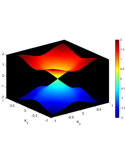
Figure 1: The dispersion relation of the self-dual interaction $H_{K}^{i}$ is shown on the left and the one on the right has broken duality with $m=0.5$ as defined in section VII.

VIII Numerical results

We also perform exact diagonalization of the DTCM on a square lattice of length $2L+1$, with both periodic and free boundary conditions. To do this, we simply use the matrix elements $h_{d^{\prime},d}(K)$ obtained in the thermodynamic limit implemented on a finite lattice. In the case of free boundary conditions, we just ignore hopping that would cause a particle to leave the finite lattice. In all numerical results, we fixed $\rho=1$, and $\lambda_{\epsilon}=\lambda_{\mu}:=\lambda$.

In Figure 2 we show the absolute value of the expansion coefficients of a bound state and a scattering of this model at $K=(\pi/4,\pi/4)$, $\lambda=0.5$, $L=60$, and using periodic boundary conditions. In the case of the bound state, we see rapid decay of the coefficients with increasing $d$, in agreement with our analysis in the previous section, implying a bound state. We also see in Figure 2 an example of a scattering state sampled from the middle of the spectrum. Generically the states in the middle of the spectrum take this form, with near equal amplitude for all values of $d$. In both these plots we have fixed $K$, but the qualitative features shown are generally true for all $K$ values that are not $0$.

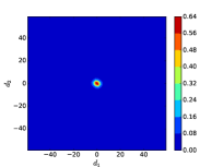
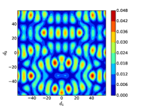
Figure 2: Plots of the expansion coefficients of the eigenstates of the DTCM for $L=60$, $\lambda=0.5$, and $K=(\pi/4,\pi/4)$. On the left we show the expansion coefficients for the bound state and on the right we show a typical scattering state found in the middle of the spectrum.

In Figure 3 we show the spectrum of the DTCM for both positive and negative values of $\lambda$, fixed $K=(\pi/4,\pi/4)$, and free boundary conditions. From chirality, the essential spectrum is invariant under $\lambda\rightarrow-\lambda$, but the effect on the bound states is not. When $\lambda=0$, we have the eigenvalues from $H_{K}^{i}$, and an extensive degeneracy at $E=0$. As we tune $\lambda$, we see the response of these eigenvalues to the term $H_{K}^{0}$. We see that for $\lambda<0$, we have that the bound state enters the continuum abruptly, while for $\lambda>0$ the bound states appear to converge to the edges of the continuum band. In Figure 4 we show the $l^{\infty}$ norm of the two largest distinct eigenvalues of ${h_{K}}_{d^{\prime},d}$ as a function of $\lambda$ for varying system sizes. We see that the $l^{\infty}$ norm is robust as we vary system size as expected for a bound state. For $\lambda>0$, the magnitude of the norm decreases in a continuous manner as $\lambda$ increases, but the decrease in norm is abrupt for $\lambda<0$.

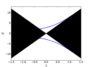
Figure 3: Plot of the spectrum of the DTCM at fixed $K=(\pi/4,\pi/4)$, $\rho=1$, and $L=30$.

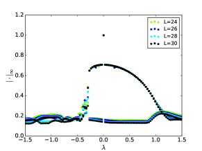
Figure 4: Plot of the $l^{\infty}$ norm of the eigenstates of the DTCM at fixed $K=(\pi/4,\pi/4)$ and $\rho=1$ at various values of the system size $L$.

Lastly, we examine the $K$-dependence of the quantity

$$V(K)=E_{\rm max}(K)-E^{0}_{\rm max}(K),$$ (37)

where $E^{0}_{\rm max}$ is the maximum eigenvalue with $\rho=0$, and $E_{\rm max}$ is the maximum eigenvalue for $\rho=1$, both found numerically at a fixed value of $K$. The quantity $V(K)$ gives a measure of the attraction of the anyons at the given system parameters. If $V(K)$ is positive, it means that the $H_{K}^{i}$ term is stronger than the $H_{K}^{0}$ term, and so a bound state is expected. If $V(K)\leq 0$, then the term $H_{K}^{0}$ dominates, and so we expect no bound state.

In Figure 5 we show $\log V(K)$ for various values of $K$ and $\lambda$, with $\rho=1$, $L=30$, and free boundary conditions. We see that for negative $\lambda$, there is a rapid decay in $V(K)$, and a cutoff where $\log V(K)$ is undefined due to $V(K)$ becoming negative. This suggests that the bound state disappears for negative $\lambda$, in agreement with Figure 3, and the analysis in Section VI. For positive $\lambda$, we see that $V(K)$ remains positive for all $\lambda$ values shown, and in fact $V(K)$ remains positive for $\lambda$ even as large as $\lambda=100$. This suggests that a bound state exists for all $\lambda>0$ for the $K$ values shown. There is a change in the slope of this curve for $\lambda\sim 1$, where the states crossover from tightly to loosely bound states. We believe that these $K$ values chosen represent the behavior for all $K$, and that the existence of a bound state for all $\lambda>0$ is true in general for arbitrary $K$. In Figure 6 we show what the maximum eigenstate looks like for $\lambda=1.5$, analogous to Figure 2. We see that in this case the expansion coefficients have appreciable magnitude for a large range of $d$ values. We believe this state is loosely bound, similar to Rydberg states in atoms.

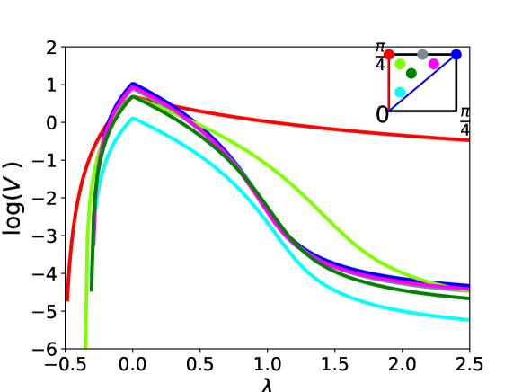
Figure 5: Plot of $V(K)$ defined in Equation 37 as a function of $\lambda$ at various $K$ values, with $\rho=1$, and $L=30$. The inset shows a color key for the $K$ values used. Note that the qualitative behavior is the same for all points on the lines $K_{x}=K_{y}$ and $k_{x}=0$, so we only choose the endpoints. The spectrum is symmetric about the line $K_{x}=K_{y}$, so we only show $K_{y}>K_{x}$.

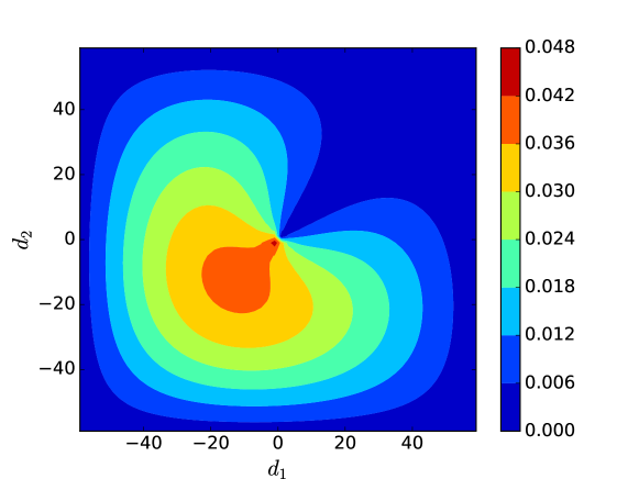
Figure 6: Plots of the expansion coefficients of the maximum eigenstate of the DTCM for $K=(\pi/4,\pi/4)$, $\lambda=1.5$ and $L=60$.

IX Discussion

We introduced a perturbation of Kitaev’s Toric Code Hamiltonian that turns the static excitations of the TCM into dynamical particles. We took care to preserve the essential symmetries of the model. In particular, the perturbations leave the minimally charged sectors invariant. We then performed a detailed analysis of the spectrum of the dynamical model in the sector charged with one electric and one magnetic anyon. We found that the ‘ribbon states’ in a certain range of the center of mass momentum are stable, i.e., exist as a bound state of one electric and one magnetic charge. At a critical value of the ratio of the parameters $\rho$ and $\lambda$ in the DTCM, the bound state eigenvalue dips into the band of scattering states, becomes unstable and the electric and magnetic anyons de-fuse into separate electric and magnetic charges.

Similar considerations can be applied to the general class of quantum double models introduced by Kitaev and other constructions of commuting Hamiltonians describing anyons.

- (1) R. Alicki, M. Fannes, and M. Horodecki, A statistical mechanics view on Kitaev’s proposal for quantum memories, J. Phys. A 40 (2007), no. 24, 6451–6467.
- (2) H. Bombin and M. A. Martin-Delgado, A family of non-abelian kitaev models on a lattice: Topological confinement and condensation, Phys. Rev. B78 (2008), 115421.
- (3) O. Bratteli and D. W. Robinson, Operator algebras and quantum statistical mechanics, 2 ed., vol. 1, Springer Verlag, 1987.
- (4) S. Bravyi, M. Hastings, and S. Michalakis, Topological quantum order: stability under local perturbations, J. Math. Phys. 51 (2010), 093512.
- (5) M. Cha, P. Naaijkens, and B. Nachtergaele, The complete set of infinite volume ground states for Kitaev’s abelian quantum double models, Commun. Math. Phys. 357 (2018), 125–157.
- (6) , On the stability of charges in infinite quantum spin systems, arXiv:1804.03203, 2018.
- (7) D. Friedan, A proof of the Nielsen-Ninomiya Theorem, Commun. Math. Phys. 85 (1982), 481.
- (8) A. Yu. Kitaev, Fault-tolerant quantum computation by anyons, Ann. Phys. 303 (2003), 2–30.
- (9) I. Klich, On the stability of topological phases on a lattice, Ann. Phys. 325 (2010), 2120–2131.
- (10) C. Knapp, E.M. Spanton, A.F Young, C. Nayak, and M.P. Zaletel, Fractional chern insulator edges and layer-resolved lattice contacts, Phys. Rev. B 99 (2019), 081114.
- (11) M. Levin and X.-G. Wen, String-net condensation: A physical mechanism for topological phases, Phys. Rev. B 71 (2005), 045110.
- (12) S. C. Morampudi, A.M. Turner, F. Pollmann, and F. Wilczek, Statistics of fractionalized excitations through threshold spectroscopy, Phys. Rev. Lett. 118 (2017), 227201.
- (13) P. Naaijkens, Localized endomorphisms in Kitaev’s toric code on the plane, Rev. Math. Phys. 23 (2011), 347–373.
- (14) H.B. Nielsen and M. Ninomiya, A no-go theorem for regularizing chiral fermions, Phys. Lett. B105 (1981), 219.
- (15) D. Takane et al., Observation of chiral fermions with a large topological charge and associated fermi-arc surface states in CoSi, Phys. Rev. Lett. 122 (2019), 076402.
- (16) J. Wang, S. Deng, Z. Liu, and Z. Liu, The rare two-dimensional materials with Dirac cones, National Science Review 2 (2015), 22–39.
- (17) R.L. Willett, C. Nayak, K. Shtengel, L.N. Pfeiffer, and K.W. West, Magnetic-field-tuned Aharonov-Bohm oscillations and evidence for non-abelian anyons at , Phys. Rev. Lett. 111 (2013), 186401.