Non-perturbative corrections to the quasiparticle velocity in graphene

Abstract

Relativistic fermionic systems have physical quantities calculated by well stablished quantum electrodynamic prescriptions. In the last few years there has been an enormous interest in condensed matter systems in which the fermions exhibit relativistic dispersion, as Dirac fermions in graphene. We employ a non-perturbative method in order to obtain a non-perturbative correction to the quasiparticle velocity in graphene, and compare with the experimental data. We find a better agreement between the quasiparticle velocity corrected with non-perturbative corrections and measurements, when compared with the standard one-loop result. We also investigate the behavior of the beta function of the renormalization group theory, and find that the non-perturbative corrections do not alter the stability of the infrared fixed point found by the standard result.

I Introduction

In condensed matter (CM) bare electrons are dressed with interactions with the many-body system, forming a “quasiparticle” Mattuck . A very interesting CM quasiparticle example happens in graphene, a promising material with extraordinary electrical, thermal and optical properties intro1 ; intro2 ; intro3 ; intro4 ; intro5 ; intro6 ; intro7 . In graphene charge carriers behave like massless relativistic particles with a conical energy spectrum $E=\hbar v_{F}k$, where $\hbar$ is the Planck’s constant divided by $2\pi$, $v_{F}$ is the Fermi velocity, which plays the role of the effective speed of light and $k$ is the wave vector. Electron-electron interactions in graphene lead to a logarithmically divergent correction to the Fermi velocity Elias .

As is well known, the naive perturbative expansion in powers of the coupling constant breaks down in some situations as, for instance, in theories with spontaneously broken symmetries requiring non-perturbative resummation schemes to obtain reliable results T1 ; T2 ; T3 . A second case happens in asymptotically free theories where one is not always able to do perturbation theory, since the coupling depends on the energy scale, and at low energies the interaction becomes strong MMarino . Finally, another example which is directly related with this work is the difficulty in conciliate the expansion of quasiparticle velocity $v_{F}(k)$ in powers of $\alpha$, the effective fine structure constant for graphene (since $\alpha=e^{2}/\hbar\kappa v_{F}\simeq 2.2$ i.e., it is greater than unity), with the experimental results Sharma . Here $\kappa$ is the dielectric constant arising from the surrounding medium. $\alpha=2.2$ is the maximum allowed value of the bare coupling strength in graphene. This value is found with $\kappa=1$ which is for graphene in vacuum, and corresponds, therefore, to the most strongly interacting graphene system Das .

As pointed out in Ref. Das2 , experiments detect a quasiparticle velocity enhancement close to the Dirac point, as reported by Elias et al. Elias , who observed a quasiparticle velocity enhancement on free-standing graphene, while perturbative renormalization group to second order shows that an unphysical fixed point in the Fermi velocity beta function appears at a critical coupling of $\alpha^{*}=0.78$ Das , indicating a decrease in the quasiparticle (Fermi) velocity $v_{F}(k)$ at low density for suspended graphene.

Motivated by these examples, in this work we investigate the effects of non-perturbative corrections to the quasiparticle velocity in a two-dimensional Dirac system. Our main goal is to calculate the zero temperature electron self-energy correction to the quasiparticle velocity $v_{F}$ in graphene in 2D (two space dimensions). We find that the second-order (in the non-perturbative calculations) results agree better with the experimental measurements than the standard (purely one-loop) result.

This paper is organized as follows. In section II we calculate the corrections to the Fermi velocity of relativistic-like quasiparticles in 2D. In this section we also study the behavior of the beta function of the renormalization group theory, and find that the non-perturbative corrections do not modify the stability of the infrared fixed point found by the standard (one-loop) result. We conclude in section III.

II The Non-perturbative Fermion Self-Energy: The MSCR

As discussed at the Introduction, it is of great importance the development of (alternative) theoretical methodologies, as non-perturbative calculations, that allow the obtention of physical quantities, principally in the situations where perturbation theory ceases to work or are not applicable.

Here we apply the Modified Self-Consistent Resummation (MSCR) procedure in order to implement a resummation of infinity sub-set of diagrams Caldas1 ; Caldas2 ; Caldas3 . The method consists in calculating the quasiparticle effective mass through consecutive iterations, assuring the mass renormalization in each step.

The divergences from the integrals computed in a present step are exactly canceled by the counter-terms that are necessary to be introduced at the previous order of the recalculation (resummation) of the self-energy to carry the renormalization. This renormalization method has been developed, originally in the context of low energy quantum chromodynamics (QCD), in Refs. Caldas1 ; Caldas2 ; Caldas3 for the resummation method employed here and has been given the name MSCR. For the purposes of this work, we initially concentrate on the full expression for $v_{F}(k)$ and refer the reader to the above cited works for a detailed treatment of the renormalization procedure.

II.0.1 Renormalization of the Quasiparticle Velocity in Graphene

Graphene is a material made of a one-atom-thick sheet of carbon, being a system where the electrons have conical valence and conduction bands, therefore behaving as massless Dirac fermions at low energies intro1 ; intro2 ; intro3 . Regarding the electron interactions in graphene, the ratio of the strength of the Coulombic interactions to the analogous quantity in QED is $\alpha_{graphene}/\alpha_{QED}\simeq 300$ effective . Because of this graphene can be considered a strong-coupling massless QED in a plane intro4 .

To calculate the one-loop renormalization of the Fermi velocity we follow closely Ref. Das , which works with the Euclidean action,

$$S\!\!\! = \!\!\!{-}\sum_{a=1}^{N}\int dtd^{2}x({\bar{\psi}}_{a}\gamma^{0}\partial_{0}\psi_{a}{+}v_{F}{\bar{\psi}}_{a}\gamma^{i}\partial_{i}\psi_{a}{+}A_{0}{\bar{\psi}}_{a}\gamma^{0}\psi_{a})$$ (1)

$$\!\!\!+{1\over 2g^{2}}\int dtd^{3}x(\partial_{i}A_{0})^{2}.$$

The action $S$ above was first used in Ref. Son to describe $2+1$ dimensional four-component massless Dirac fermions interacting through a $3$ dimensional instantaneous Coulomb interaction. In Eq. (1), $v_{F}\approx c/300$ is the bare Fermi velocity of the Dirac quasiparticles in graphene. The fields ${\bar{\psi}}_{a}$ are four-component fermion fields describing electrons and holes, with $a$ labeling the fermion species. The number of species, $N$, is equal to 2 in real graphene, corresponding to the spin degeneracy. The $\gamma$’s are Dirac matrices satisfying the Euclidean Clifford algebra, $\{\gamma^{\mu},\gamma^{\nu}\}=2\delta^{\mu\nu}$, which can be chosen as

$$\gamma^{0}=\sigma_{3}\otimes\sigma_{3},\qquad\gamma^{i}=\sigma_{i}\otimes I,$$ (2)

where the $\sigma_{i}$ are Pauli matrices.

The coupling $g^{2}$ is given by

$$g^{2}={2\over 1+\epsilon}{e^{2}\over\epsilon_{0}}=\frac{4\pi e^{2}}{\kappa},$$ (3)

where $e$ is the electric charge, $\epsilon_{0}$ is the vacuum permeability, and $\epsilon$ and $\kappa$ are two different definitions of the dielectric constant of the substrate (SI and cgs units, respectively). Associating these quantities with the Fermi velocity, one can define,

$$\alpha\equiv\frac{g^{2}}{4\pi v_{F}}=\frac{e^{2}}{2\pi(1+\epsilon)\epsilon_{0}v_{F}}=\frac{e^{2}}{\kappa v_{F}}.$$ (4)

It is appropriate to make use of the quasirelativistic notation,

$$\not{p}=\gamma^{0}p_{0}+v_{F}\vec{\gamma}\cdot\vec{p},\qquad p^{2}=p_{0}^{2}+v_{F}^{2}|\vec{p}|^{2}.$$ (5)

The propagator of a massless free fermion is given by

$$G_{0}(p)=\frac{i}{\not{p}}=\frac{i\not{p}}{p^{2}},$$ (6)

while the effective propagator for the Coulomb interaction reads

$$D_{0}(p)=g^{2}\int\frac{dp_{z}}{2\pi}\frac{1}{p_{z}^{2}+|\vec{p}|^{2}}=\frac{g^{2}}{2|\vec{p}|},$$ (7)

and the interaction vertex is $i\gamma^{0}$. Every closed fermion loop contributes an overall minus sign to the value of the diagram.

The one-loop diagram has been evaluated several times in the literature, and following Ref. Das in Appendix A, we find

$$\Sigma_{1}(q)=\frac{ig^{2}}{16\pi}\vec{q}\cdot\vec{\gamma}\log(\Lambda/|\vec{q}|),$$ (8)

where $\Lambda$ is an ultraviolet cut-off. For the case of graphene, the physical cut-off is $\Lambda\approx 1/a$, with $a$ being the graphene lattice constant, and represents the momentum scale up to which the spectrum is Dirac-like Kotov .

Since the full fermion propagator is given by

$$G(p)=\frac{i}{\not{p}-i\Sigma(p)},$$ (9)

the one-loop self-energy leads to a renormalization of the quasiparticle velocity,

$$v_{q} \equiv v_{F}^{*}(q)$$ (10)

$$= v_{F}+\frac{g^{2}}{16\pi}\log(\Lambda/|\vec{q}|)$$

$$= v_{F}\left[1+\frac{\alpha}{4}\log(\Lambda/|\vec{q}|)\right],$$

meaning that the quasiparticle velocity increases, since $\alpha>0$ and $\Lambda/|\vec{q}|\gg 1$.

With the aid of Eq. (3), and with $v_{q}$ in Eq. (10) an equation for the coupling as a function of the momentum and the bare coupling can be obtained

$$\frac{\alpha_{q}}{\alpha}=\frac{1}{1+\frac{\alpha}{4}\log(\Lambda/|\vec{q}|)}=\frac{v_{F}}{v_{q}}.$$ (11)

in order to eliminate the arbitrary ultraviolet momentum cutoff $\Lambda$ can find Das2 expressions akin to those above in another momentum, say $k$

$$\frac{\alpha_{k}}{\alpha}=\frac{1}{1+\frac{\alpha}{4}\log(\Lambda/|\vec{k}|)}=\frac{v_{F}}{v_{k}}.$$ (12)

Instead of defining a velocity ratio as in Ref. Das , which still depends on $\Lambda$ through $\alpha_{k}$ ($\frac{v_{q}}{v_{k}}=1+\frac{\alpha_{k}}{4}\log(|\vec{k}|/|\vec{q}|)$, with $\alpha_{k}$ given by Eq. (12)), we define a velocity difference, which is independent of $\Lambda$,

$$\frac{\alpha}{\alpha_{q}}-\frac{\alpha}{\alpha_{k}}=\frac{v_{q}-v_{k}}{v_{F}}=\frac{\alpha}{4}\log(|\vec{k}|/|\vec{q}|),$$ (13)

which relates the difference between the physical velocities at momentum $|\vec{q}|$ and $|\vec{k}|$, respectively, with no cutoff $\Lambda$ dependence.

II.0.2 One-loop Renormalization Group Analysis

Let us now apply renormalization group (RG) theory by considering the effect of changing the momentum scale $q=|\vec{q}|$ of $v_{q}$ in Eq. (10). From Eq. (13) we can obtain the beta function for the effective coupling, by means of the renormalization group equation

$$\beta(\bar{\alpha})=k\frac{\partial\bar{\alpha}}{\partial k}=-\frac{1}{4}\frac{1}{\left(\frac{1}{4}\log(k/q)\right)^{2}},$$ (14)

where $k=|\vec{k}|$, and from Eq. (13) we have defined $\frac{1}{\bar{\alpha}}\equiv\frac{1}{\alpha_{q}}-\frac{1}{\alpha_{k}}$. Integration of the above $\beta(\bar{\alpha})$ equation gives

$$\frac{1}{\bar{\alpha}(k)}-\frac{1}{\bar{\alpha}(q)}=\frac{1}{4}\ln\left(\frac{k}{q}\right),$$ (15)

which shows that the coupling strength $\bar{\alpha}(k)$ decreases with increasing $k$.

Notice that from Eq. (14) we have

$$\beta(\bar{\alpha})=-\frac{1}{4}\bar{\alpha}^{2}.$$ (16)

This result tells us that a (trivial) fixed point (FP) occurs at $\bar{\alpha}=\bar{\alpha}_{c}=0$. This FP is stable, since

$$\frac{d\beta(\bar{\alpha})}{d\bar{\alpha}}|_{\bar{\alpha}=\bar{\alpha}_{c}}=0.$$ (17)

This stable FP corresponds to an infrared (IR) point, since it is reached through the limit $q\to 0$ Kotov .

In Fig. 1 we show the behavior of the coupling strength $\bar{\alpha}$, and the $\beta(\bar{\alpha})$ function from Eqs. (15) and (16), respectively, as a function of $\lambda\equiv k/q$. Both functions vanish at the limit $\lambda\to\infty$. On the other hand, this also means that the renormalized quasiparticle velocity $v\equiv(v_{q}-v_{k})/v_{F}\propto\bar{\alpha}^{-1}$ diverges in this limit. The renormalized quasiparticle velocity $v(\bar{\alpha})$ is also shown in Fig. 1. The functions $\alpha(\lambda_{UV})$ and $\beta(\bar{\alpha}(\lambda_{UV}))$ diverge at the ultraviolet point $\lambda=\lambda_{UV}=1$. At this UV point $v$ is zero. Lastly, at the (unattainable) point $\lambda=0$, $\bar{\alpha}(\lambda=0)=\beta(\bar{\alpha}(\lambda=0))=0$, and $v$ diverges to $-\infty$.

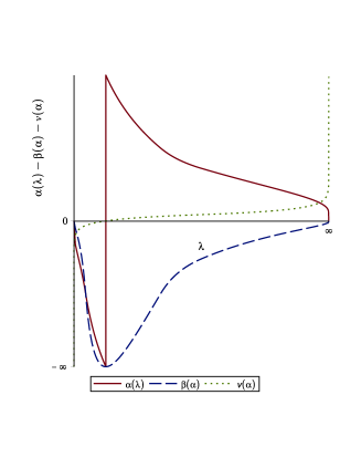
Figure 1: Behavior of the one-loop coupling strength $\bar{\alpha}$, the $\beta(\bar{\alpha})$ function and the renormalized Fermi velocity $v\propto 1/\bar{\alpha}$, as a function of $\lambda=k/q$.

II.0.3 The Non-perturbative Electron Quasiparticle Velocity in Graphene

We now obtain the non-perturbative corrections to the renormalization of the quasiparticle velocity we have just obtained up to second-order in the iterations.

As is well known, owing to the massless character of electrons in the model described by Eq. (1), it is sensitive to retardation effects of the electromagnetic propagation GonzalezNPB94 . In static models like this, with an instantaneous photon propagator i.e., corresponding to $c=\infty$, the Fermi velocity grows without bound (in opposition to what happens in the retarded - corresponding to $c$ finite - model GonzalezNPB94 ) in the infrared V-Guinea . Thus, the use of the non-retarded action $S$ (with such an instantaneous long range Coulomb interaction) in Eq. (1) deserves some comments on it. As pointed out in Ref. GonzalezNPB94 , one should not expect any discrepancy in the computation of local quantities, i.e., cutoff dependent ones, in a non-retarded and in a retarded model in the limit $v_{F}/c\to 0$. However, different results should be noticeable in the computation of nonlocal quantities, due to the dissimilar forms of the interactions in the infrared regime GonzalezNPB94 . In addition, because of the mentioned infrared instabilities, perturbation theory looses its predictive power and other methods (such as the non-perturbative MSCR) may be employed. There are some particular cases in which retardation effects are not important as, for instance, that of Van der Waals interactions. In fact, it was demonstrated in Ref. Gomes that retardation effects has little significance in undoped graphene, for both zero and finite temperature. It is also worth to mention that in the investigation of finite-temperature Casimir effects for graphene, the transition from the retarded regime to a non-retarded one, happens at separations characterized by a material wavelength Ignat .

Proceeding as before, we define $v_{F}^{*}(q)$ in Eq. (10) as $v_{F1}(q)$, and obtain $\Sigma_{2}=\Sigma_{2}(v_{F1}(q))$,

$$\Sigma_{2}(v_{F1}(q))=\frac{i\alpha}{4}v_{F1}(q)\vec{q}\cdot\vec{\gamma}\log(\Lambda/|\vec{q}|).$$ (18)

Inserting the above equation into Eq. (9), we obtain

$$v_{F2}(q) = v_{F}+v_{F1}(q)\frac{\alpha}{4}\log(\Lambda/|\vec{q}|)\to$$

$$\frac{v_{F2}(q)}{v_{F}} = 1+\frac{\alpha}{4}\log(\Lambda/|\vec{q}|)+\left(\frac{\alpha}{4}\right)^{2}\left[\log(\Lambda/|\vec{q}|)\right]^{2},$$ (19)

where we have made use of Eq. (10). The MSCR is somewhat very close to the DuBois’s approach, i.e., an iteration-perturbation method, which generates a series of iterations Dubois .

The behavior of $v_{F2}$ as a function of the density $n$ can be investigated by noticing that the Fermi momentum is proportional to the square root of the carrier density, $q_{F}=(\pi n)^{1/2}$, while the momentum cutoff $\Lambda=(\pi n_{c})^{1/2}$, with a fixed reference density $n_{c}=10^{15}cm^{-2}$ Das . Then we find

$$\frac{v_{F2}(n)}{v_{F}} = 1+\frac{\alpha}{8}\log\left(\frac{n_{c}}{n}\right)+\frac{1}{4}\left(\frac{\alpha}{4}\right)^{2}\left[\log\left(\frac{n_{c}}{n}\right)\right]^{2}.$$ (20)

In order to compare $v_{F2}(n)$ obtained above with the experimental measurements of the renormalized Fermi velocity for suspended graphene, we employ the same approximation used in Ref. Elias to take into account the screening by graphene’s charge carriers. This approach is implemented by defining an effective screening constant $\epsilon_{G}$ such that $\alpha\to\alpha/\epsilon_{G}$ in Eq. (20). The whole range of $n$ in Ref. Elias had a best fit for $\epsilon_{G}\sim 3.5$. In Fig. 2 we show $v_{F1}(n)$ and $v_{F2}(n)$ for $\alpha=2.2$ and $\epsilon_{G}\sim 3.5$, where $v_{F1}(n)$ (dashed curve) is the standard one-loop result, while $v_{F2}(n)$, calculated with the second-order of the iteration within MSCR, is the solid curve. $v_{F2}(n)$ shows a much better agreement (as compared to $v_{F1}(n)$) with the experimental data points, obtained in Ref. Elias .

Notice that the renormalized Fermi velocity for graphene deposited on a substrate shows the same (qualitative) behavior as for suspende graphene. See, for instance, Ref. Yu , where, for graphene on a substrate, $\alpha<2.2$, which corresponds to a dielectric constant $\kappa>1$ Das .

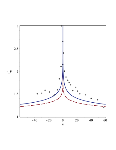
Figure 2: Behavior of the Fermi velocity $v_{F1}(n)$, dashed curve, and $v_{F2}(n)$, solid curve, (plotted in units of $10^{6}ms^{-1}$), as a function of carrier density $n$ (in units of $10^{12}cm^{-2}$). The experimental data points are taken from Ref. Elias .

As pointed out in Ref. Sharma , it is worth mentioning that the renormalization of the Fermi velocity has been computed to second-order of perturbation theory (in powers of the dimensionless interaction constant) and conflicting results have been found as, for example, in Ref. Mish , it was found

$$v_{F}(q)=v_{F}\left\{1+\left[\frac{g_{0}}{4}-g_{0}^{2}\left(\frac{5}{6}-\ln 2\right)\right]\log(\Lambda/|\vec{q}|)\right\},$$ (21)

where $g_{0}=e^{2}/\kappa\nu_{0}$, where $\kappa$ is the dielectric constant of a substrate and $\nu_{0}$ is the bare electron velocity, then $g_{0}=\alpha$, and in Ref. Das

$$v_{F}(q)=v_{F}\left\{1+\left[\frac{\alpha}{4}+\alpha^{2}\left(\frac{3\log 2-4}{6}\right)\right]\log(\Lambda/|\vec{q}|)\right\}.$$ (22)

Actually, the above result is formed by the first term of a general expression found in Ref. Das

$$\frac{v_{F}(q)}{v_{F}}=1+\sum_{n=1}^{\infty}F_{n}(\alpha)\log^{n}(\Lambda/|\vec{q}|),$$ (23)

where $F_{1}(\alpha)=f_{1}\alpha+f_{2}\alpha^{2}$, with $f_{1}=\frac{1}{4}$, and $f_{2}=\frac{3\log 2-4}{6}$. Eq. (23) is an indicative of breakdown of perturbation theory.

II.0.4 One-loop plus Non-perturbative Corrections Renormalization Group Analysis

From Eq. (19) we can obtain the momentum-dependent coupling constant

$$\frac{\alpha_{q2}}{\alpha}=\frac{1}{1+\frac{\alpha}{4}\log(\Lambda/q)+\left(\frac{\alpha}{4}\right)^{2}\left[\log(\Lambda/q)\right]^{2}}.$$ (24)

The difference of the inverse of the coupling at two different momenta, gives

$$\frac{\alpha}{\alpha_{2q}}-\frac{\alpha}{\alpha_{2k}}=\frac{v_{F2}(q)-v_{F2}(k)}{v_{F}}=$$ (25)

$$\frac{\alpha}{4}\log(k/q)+\left(\frac{\alpha}{4}\right)^{2}\left[(\log(\Lambda/q))^{2}-(\log(\Lambda/k))^{2}\right].$$

Defining $\frac{1}{\bar{\alpha}_{2}}\equiv\frac{1}{\alpha_{2q}}-\frac{1}{\alpha_{2k}}$ as we did at one-loop, we find a beta function for the effective coupling

$$\beta(\bar{\alpha}_{2})=k\frac{\partial\bar{\alpha}_{2}}{\partial k}$$

$$= -\frac{1}{4}\frac{\left[1+\frac{\alpha}{2}\log(\Lambda/k)\right]}{\left[\frac{1}{4}\log(k/q)+\frac{\alpha}{16}\left((\log(\Lambda/q))^{2}-(\log(\Lambda/k))^{2}\right)\right]^{2}}$$

$$= -\frac{1}{4}\left[1+\frac{\alpha}{2}\log(\Lambda/k)\right]\bar{\alpha}_{2}^{2}.$$

As happens at one-loop, a fixed point occurs at $\bar{\alpha}_{2}=\bar{\alpha}_{2c}=0$. Thus, up to second-order of the non-perturbative iteration we do not find any fixed point $\bar{\alpha}_{2}\neq 0$. Again, this is a stable IR-FP, since

$$\frac{d\beta(\bar{\alpha}_{2})}{d\bar{\alpha}_{2}}|_{\bar{\alpha}_{2}=\bar{\alpha}_{2c}}=0.$$ (27)

III Summary

To summarize, we have investigated the effect of non-perturbative corrections to the Fermi velocity in graphene. Interestingly, we find that although the electrons near the Dirac points (i.e., the contact points between the valence and conduction bands) in graphene have the well known Dirac dispersion, the evolution of their coupling with momentum (energy) scale reveals a behavior of many non-abelian gauge theories, as QCD, possessing a negative $\beta$ function. We find that both the first and second-order results of the non-perturbative calculation shown in Fig. 2 are in qualitative agreement with the experimental data obtained in Ref. Elias . However, the second-order result of the non-perturbative calculation is in quantitative agreement with the measurements of the Fermi velocity renormalization in suspended graphene, taken from Ref. Elias .

We also investigated the behavior of the $\beta$ function of the renormalization group theory, and find that the non-perturbative corrections do not modify the stability of the infrared fixed point found by the standard (one-loop) result.

Our approach might also be useful in the investigation of various physical quantities, in graphene and other similar fermion systems. The study of the non-perturbative corrections to the effective mass and consequently to the pairing gap of a 1d fermion system is in progress and will be presented elsewhere.

IV Acknowledgments

We would like to thank E. Barnes and J. Hofmann for helpful discussions. The author acknowledges partial support by CNPq-Brazil and FAPEMIG.

Appendix A Explicit calculation of the one-loop electron self-energy in graphene

The one-loop electron self-energy diagram was originally evaluated in Ref. GonzalezNPB94 , however, we follow the steps from Ref. Das . The diagram is written as

$$\Sigma_{1}(q) = -\int\frac{d^{3}k}{(2\pi)^{3}}\gamma^{0}G_{0}(k+q)\gamma^{0}D_{0}(k)$$ (28)

$$= -\frac{ig^{2}}{2}\int\frac{d^{3}k}{(2\pi)^{3}}\gamma^{0}\frac{\not{k}+\not{q}}{(k+q)^{2}}\gamma^{0}\frac{1}{|\vec{k}|}$$

$$= -\frac{ig^{2}}{2}\int\frac{d^{2}k}{(2\pi)^{2}}\frac{1}{|\vec{k}|}\gamma^{0}K(q,\vec{k})\gamma^{0},$$

$$K(q,\vec{k}) = \int\frac{dk_{0}}{2\pi}\frac{\not{k}+\not{q}}{(k+q)^{2}}$$ (29)

$$= \int\frac{dk_{0}}{2\pi}\left[\frac{v_{F}(\vec{k}+\vec{q})\cdot\vec{\gamma}}{k_{0}^{2}+v_{F}^{2}|\vec{k}+\vec{q}|^{2}}+\frac{k_{0}\gamma^{0}}{k_{0}^{2}+v_{F}^{2}|\vec{k}+\vec{q}|^{2}}\right]$$

$$= \frac{(\vec{k}+\vec{q})\cdot\vec{\gamma}}{2|\vec{k}+\vec{q}|},$$

$$\Sigma_{1}(q)=\frac{ig^{2}}{4}\int\frac{d^{2}k}{(2\pi)^{2}}\frac{1}{|\vec{k}|}\frac{(\vec{k}+\vec{q})\cdot\vec{\gamma}}{|\vec{k}+\vec{q}|}.$$ (30)

In order to perform the remaining integrals, we choose the coordinate system such that $\vec{q}=(|\vec{q}|,0)$. As in Ref. Das , we adopt the transformation to elliptical coordinates

$$k_{x}=\frac{|\vec{q}|}{2}(\cosh\mu\cos\nu-1),\qquad k_{y}=\frac{|\vec{q}|}{2}\sinh\mu\sin\nu,$$

$$d^{2}k=\frac{|\vec{q}|^{2}}{4}(\cosh^{2}\mu-\cos^{2}\nu)d\mu d\nu,$$ (31)

yielding

$$\!\!\!\!\!\!\Sigma_{1}(q)=$$

$$\!\!\!\!\!\!\frac{ig^{2}|\vec{q}|}{32\pi^{2}}\gamma\cdot\int_{0}^{2\pi}d\nu\int_{0}^{\mu_{max}}d\mu(1+\cos\nu\cosh\mu,\sin\nu\sinh\mu).$$

(32)

The integral has been regulated by including the cutoff, $\mu_{max}$. We would like to relate this cutoff to a more physical cutoff on the momentum: $\Lambda\geq|\vec{k}|$. The mapping to elliptical coordinates given above implies

$$|\vec{k}|=\frac{|\vec{q}|}{2}(\cosh\mu-\cos\nu),$$ (33)

so that

$$\Lambda=\frac{|\vec{q}|}{2}(\cosh\mu_{max}-\cos\nu)$$

$$\Rightarrow\mu_{max}=\cosh^{-1}\left(\frac{2\Lambda}{|\vec{q}|}+\cos\nu\right).$$ (34)

The three integrals in (32) then evaluate to

$$\!\!\!\!\!\!{\int_{0}^{2\pi}}d\nu{\int_{0}^{\mu_{max}}}d\mu={\int_{0}^{2\pi}}d\nu\cosh^{{-}1}\left(\frac{2\Lambda}{|\vec{q}|}{+}\cos\nu\right)$$

$$=2\pi\log(4\Lambda/|\vec{q}|){+}O(|\vec{q}|^{2}/\Lambda^{2}),$$

$$\!\!\!\!\!\!{\int_{0}^{2\pi}}d\nu\cos\nu{\int_{0}^{\mu_{max}}}d\mu\cosh\mu$$

$$={\int_{0}^{2\pi}}d\nu\cos\nu\sqrt{\left(\frac{2\Lambda}{|\vec{q}|}{+}\cos\nu\right)^{2}{-}1}=\pi{+}O(|\vec{q}|^{2}/\Lambda^{2}),$$

$$\!\!\!\!\!\!{\int_{0}^{2\pi}}d\nu\sin\nu{\int_{0}^{\mu_{max}}}d\mu\sinh\mu$$

$$={\int_{0}^{2\pi}}d\nu\sin\nu\left(\frac{2\Lambda}{|\vec{q}|}{+}\cos\nu\right)=0.$$ (35)

Plugging these results into (32), and reverting to a general coordinate system, i.e., $\vec{q}=(q_{x},q_{y})$, one finally obtains

$$\Sigma_{1}(q)\!\!\! {=} \!\!\!\frac{ig^{2}|\vec{q}|}{32\pi^{2}}\gamma^{1}\left[2\pi\log(\Lambda/|\vec{q}|){+}4\pi\log 2{+}\pi\right]{+}O\left(\frac{|\vec{q}|^{2}}{\Lambda^{2}}\right)$$

$$\rightarrow \!\!\!\frac{ig^{2}}{16\pi}\vec{q}\cdot\vec{\gamma}\left[\log(\Lambda/|\vec{q}|){+}2\log 2{+}1/2\right]{+}O\left(\frac{|\vec{q}|^{2}}{\Lambda^{2}}\right).$$

Then we have,

$$\Sigma_{1}(q)=\frac{ig^{2}}{16\pi}\vec{q}\cdot\vec{\gamma}\log(\Lambda/|\vec{q}|),$$ (37)

which is the self-energy in Eq. (8). In the above equation the finite part ($2\log 2+1/2$) has been absorbed into a redefinition of the ultraviolet momentum cutoff $\Lambda$.

References

- (1) Richard D. Mattuck, A Guide to Feynman Diagrams in the Many-Body Problem, New York, McGraw-Hill (1976).
- (2) K. S. Novoselov, A. K. Geim, S. V. Morozov, D. Jiang, M. I. Katsnelson, I. V. Grigorieva, S. V. Dubonos, and A. A. Firsov, Nature (London) 438, 197 (2005).
- (3) Y. Zhang, Y.-W. Tan, H. L. Stormer, and P. Kim, Nature (London) 438, 201 (2005).
- (4) N. M. R. Peres, F. Guinea, and A. H. Castro Neto, Phys. Rev. B 72, 174406 (2005).
- (5) A. K. Geim, and K. S. Novoselov, Nature Mater. 6, 183 (2007).
- (6) A. K. Geim and A. H. MacDonald, Physics Today 60, 35-41 (2007).
- (7) A. H. Castro Neto, F. Guinea, N. M. R. Peres, Phys. World 19, 33 (2006).
- (8) A. H. Castro Neto, F. Guinea, N. M. R. Peres, K. S. Novoselov, and A. K. Geim, Rev. Mod. Phys. 81, 109 (2009).
- (9) D. C. Elias, R. V. Gorbachev, A. S. Mayorov, S. V. Morozov, A. A. Zhukov, P. Blake, L. A. Ponomarenko, I. V. Grigorieva, K. S. Novoselov, F. Guinea, and A. K. Geim, Nat. Phys. 7, 701 (2011).
- (10) D. A. Kirzhnits and A. D. Linde, Phys. Lett. B42, 471 (1972); Ann. Phys. 101, 195 (1976).
- (11) L. Dolan and R. Jackiw, Phys. Rev. D 9, 3320 (1974).
- (12) S. Weinberg, Phys. Rev. D 9, 3357 (1974).
- (13) M. Mariño, Instantons and Large N: An Introduction to Non-Perturbative Methods in Quantum Field Theory, Cambridge, Cambridge University Press (2015).
- (14) A. Sharma and P. Kopietz, Phys. Rev. B 93, 235425 (2016).
- (15) E. Barnes, E. H. Hwang, R. E. Throckmorton, and S. Das Sarma, Phys. Rev. B 89, 235431 (2014).
- (16) J. Hofmann, E. Barnes, and S. Das Sarma Phys. Rev. Lett. 113, 105502 (2014).
- (17) H. Caldas, A. L. Mota and M. C. Nemes, Phys. Rev. D 63, 56011 (2001).
- (18) H. Caldas, Phys. Rev. D 65, 65005 (2002).
- (19) H. Caldas, Phys. Rev. D 66, 105015 (2002).
- (20) J. P. Reed, B. Uchoa, Y. I. Joe, Y. Gan, D. Casa, E. Fradkin, and P. Abbamonte, Science 330, 805 (2010).
- (21) D. T. Son, Phys. Rev. B 75, 235423 (2007).
- (22) V. N. Kotov, B. Uchoa, V. M. Pereira, F. Guinea, and A. H. Castro Neto, Rev. Mod. Phys. 84, 1067 (2012).
- (23) J. Gonzalez, F. Guinea, and M. A. H. Vozmediano, Nucl. Phys. B 424, 595 (1994).
- (24) M. A. H. Vozmediano, F. Guinea, Phys. Scr. T146, 014015 (2012).
- (25) G. Gómez-Santos, Phys. Rev. B, 80, 245424 (2009).
- (26) I. V. Fialkovsky, V. N. Marachevsky, and D. V. Vassilevich, Phys. Rev. B 84, 035446 (2011).
- (27) D. F. DuBois, Ann. Phys. (N. Y.) 7, 174 (1959); 8, 24 (1959).
- (28) G. L. Yu, R. Jalil, B. Belle, A. S. Mayorov, P. Blake, F. Schedin, S. V. Morozov, L. A. Ponomarenko, F. Chi- appini, S. Wiedmann, et al., Proc. Natl. Acad. Sci. USA 110, 3282 (2013).
- (29) E. G. Mishchenko, Phys. Rev. Lett. 98, 216801 (2007).