Sparse Array Design for Maximizing the Signal-to-Interference-plus-Noise-Ratio by Matrix Completion

Abstract

We consider sparse array beamfomer design achieving maximum signal-to interference plus noise ratio (MaxSINR). Both array configuration and weights are attuned to the changing sensing environment. This is accomplished by simultaneously switching among antenna positions and adjusting the corresponding weights. The sparse array optimization design requires estimating the data autocorrelations at all spatial lags across the array aperture. Towards this end, we adopt low rank matrix completion under the semidefinite Toeplitz constraint for interpolating those autocorrelation values corresponding to the missing lags. We compare the performance of matrix completion approach with that of the fully augmentable sparse array design acting on the same objective function. The optimization tool employed is the regularized $l_{1}$-norm successive convex approximation (SCA). Design examples with simulated data are presented using different operating scenarios, along with performance comparisons among various configurations.

1 Introduction

Sensor selection schemes strive to optimize various performance metrics while curtailing valuable hardware and computational resources. Sparse sensor placement, with various design objectives, has successfully been employed in diverse application areas, particularly for enhanced parameter estimation and receiver performance [1, 2, 3, 4, 5, 6, 7, 8]. The sparse array design criteria are generally categorized into environment-independent and environment-dependent performance metrics. The former are largely benign to the underlying environment and, in principle, seek to maximize the spatial degrees of freedom by extending the co-array aperture. This enables high resolution direction of arrival (DOA) estimation possibly involving more sources than the available physical sensors [9, 10, 11, 12, 13]. Environment-dependent objectives, on the other hand, consider the operating conditions characterized by emitters and targets in the array field of view, in addition to receiver noise. In this regard, applying such objectives renders the array configuration as well as the array weights time-varying in response to dynamic and changing environment.

In this paper, we focus on optimum sparse array design for receive beamforming that maximizes the output signal-to-interference and noise ratio (MaxSINR) [14, 15, 16]. It has been shown that optimum sparse array beamforming involves both array configuration and weights, and can yield significant dividends in terms of SINR performance in presence of desired and interfering sources [17, 18, 19, 20, 21, 22, 23]. However, one key challenge in implementing the data-dependent approaches, like Capon beamforming, is the need to have the exact or estimated values of the data autocorrelation function across the full sparse array aperture [14, 24]. This underlying predicament arises as the sparse array design can only have few active sensors at a time, in essence making it difficult to furnish the correlation values corresponding to the inactive sensor locations.

To address the aforementioned problem, we propose in this paper a matrix completion strategy assuming a single desired source and multiple interfering sources. This strategy permits the interpolation of the missing data correlation lags, thus enabling optimum “thinning” of the array for MaxSINR. The low rank matrix completion has been utilized successfully in many applications, including the high-resolution direction of arrival estimation. We compare the matrix completion strategy to the hybrid sparse array design that has been recently introduced and which also provides full spatial autocorrelation function for array thinning [25]. The fundamental thrust of the hybrid design is to pre-allocate some of the available sensors in such a way so as to ensure that all possible correlation lags can be estimated. In this case, the difference between the available sensors and those pre-allocated can be utilized for maximum SINR. In essence, the hybrid design locks few spatial degrees of freedom in an attempt to making the full autocorrelation matrix available to carry out the array optimization at all times. In that sense, it is a hybrid between structured and non-structured arrays. With pre-allocated sensors, the design approach offers a simplified antenna switching as the environment changes. In contrast, the matrix completion-based design is not tied in to any pre-allocated sensor position and, therefore, has the ability to optimize over all the available sensor locations. However, low rank matrix completion is a pre-processing step that is required every time we decide on sensor selection as the environment changes. This significantly adds to the overall overhead and computational complexity. We examine both approaches using estimated autocorrelation function, in lieu of its exact values, and compare their respective performances under different settings and degrees of freedom.

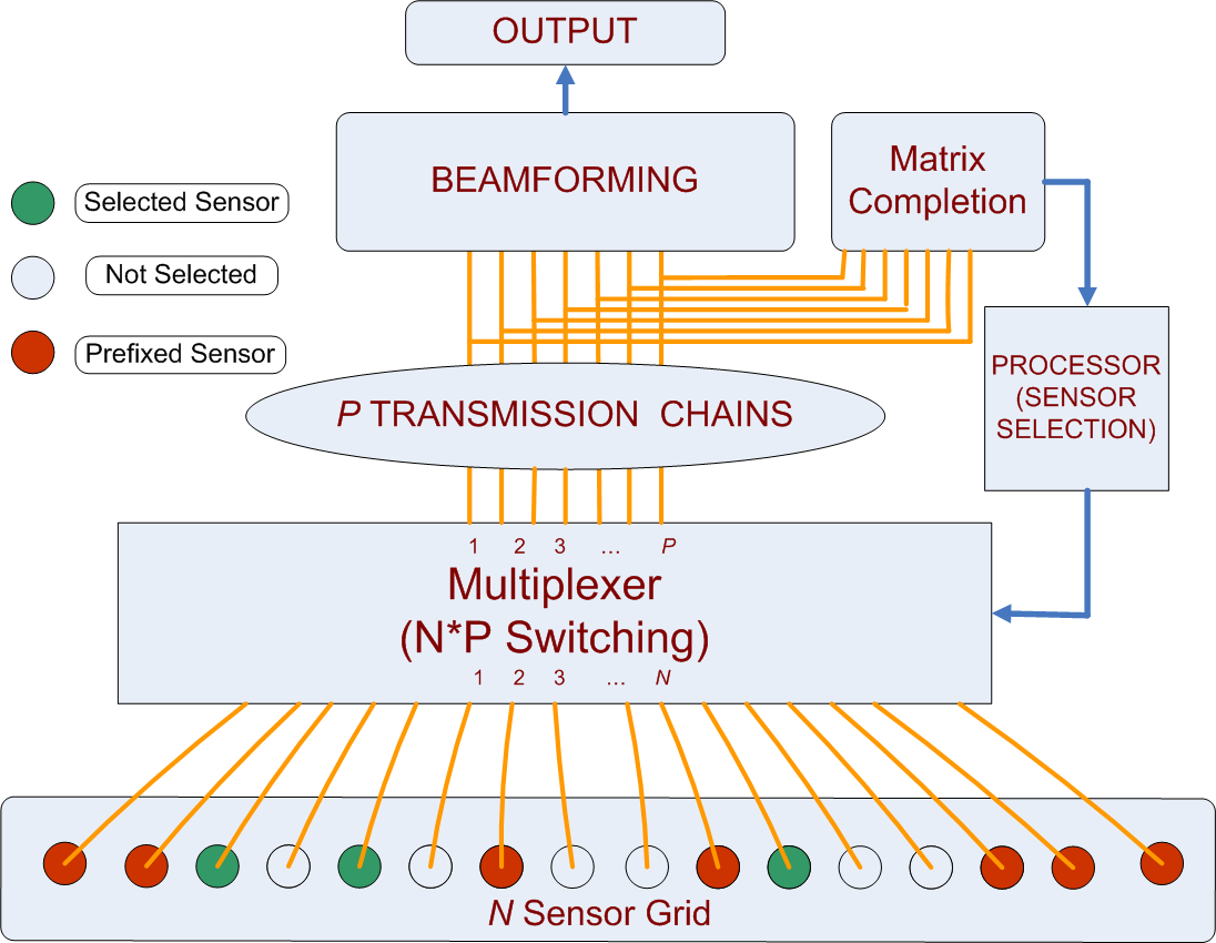
Figure 1: Block diagram implementing adaptive beamforming and antenna switching

It is worth noting that MaxSINR sparse array design using either is an entwined optimization problem that jointly optimizes the beamforming weights and determines the active sensor locations. The optimization is posed as finding $P$ sensor positions out of $N$ possible equally spaced grid points for the highest SINR performance. It is known that maximizing the SINR is equivalent to the problem of maximizing the principal eigenvalue of the product of the inverse of data correlation matrix and the desired source correlation matrix [24]. However, the maximum eigenvalue problem over all possible sparse topologies is a combinatorial problem and is challenging to solve in polynomial times. To alleviate the computational complexity of exhaustive combinatorial search, we pose this problem as successive convex approximation (SCA) with reweighted $l_{1}$-norm regularization to promote sparsity in the final solution.

To proceed with the SCA optimization, it is essential to input the algorithm with the full data correlation matrix. For the hybrid design, all the correlation lags are available and, therefore, we resort to averaging across the available correlation lags to harness a Toepltiz matrix estimate of the received data. On the other hand, a sparse array designed freely without preallocating sensor locations necessitates the use of low rank matrix completion to interpolate the missing lags and subsequently applying the SCA optimization [26]. The word “free” implies no preset position of any of the sensors involved. It is shown that the matrix completion is an effective approach to accomplish the MaxSINR sparse design. The performance of matrix completion can potentially surpass the hybrid design at the expense of more involved sensor switching and additional computational complexity stemming from the Toeplitz interpolation of the missing correlation lags.

The rest of the paper is organized as follows: In the next section, we state the problem formulation for maximizing the output SINR. Section 3 details the SCA for arrays designed freely alongside the hybrid design approach and the associated modified SCA optimization. Section 4 explains the matrix completion approach. In section 5, with the aid of Monte Carlo simulations, we compare the performance of hybrid-designed arrays viz a viz freely-designed arrays in a limited snapshot environment. Concluding remarks follow at the end.

2 Problem Formulation

We consider an emitter source in the presence of narrowband interfering signals. The signals impinge on a uniform grid of $N$ linear elements with the inter-element spacing of $d$ and the received signal is given by;

$$\mathbf{x}(n)=b_{s}(n)\mathbf{s}(\theta)+\sum_{k=1}^{I}b_{ik}(n)\mathbf{i}(\theta_{k})+\mathbf{v}(n),$$ (1)

The sampling instance is $n$, $I$ are the number of interfering sources and ($b_{s}(n)$, $b_{ik}(n))$ $\in\mathbb{C}$ are the baseband signals for the source and interferences, respectively. The steering vector corresponding to the direction of arrival of desired source $\mathbf{s}({\theta})$ $\in\mathbb{C}^{N}$ is given by,

$$\mathbf{s}({\theta})=[1\,\,\,e^{j(2\pi/\lambda)dcos(\theta)}\,.\,.\,.\,e^{j(2\pi/\lambda)d(N-1)cos(\theta)}]^{T}.$$ (2)

The interference steering vectors $\mathbf{i}({\theta_{k}})$ are similarly defined. The additive noise $\mathbf{v}(n)$ $\in\mathbb{C}^{N}$ is Gaussian with variance $\sigma_{v}^{2}$. The beamformer processes the received signal $\mathbf{x}(n)$ linearly to improve SINR. The beamformer output $y(n)$ is given by,

$$y(n)=\mathbf{w}_{o}^{H}\mathbf{x}(n),$$ (3)

The optimal beamforming weights $\mathbf{w}_{o}$ that maximizes SINR is given by solving the following optimization problem [24];

$$\underset{\mathbf{w}\in\mathbb{C}^{N}}{\text{minimize}} \quad\mathbf{w}^{H}\mathbf{R}_{i}\mathbf{w},$$ (4)

s.t. $$\quad\mathbf{w}^{H}\mathbf{R}_{s}\mathbf{w}=1.$$

The desired source correlation is $\mathbf{R}_{s}=\sigma^{2}\mathbf{s}(\theta)\mathbf{s}^{H}(\theta)$, with source power $\sigma^{2}=E\{b_{s}(n)b_{s}^{H}(n)\}$. The sum of the interference and uncorrelated noise correlation matrix is $\mathbf{R}_{i}=\sum_{k=1}^{I}(\sigma^{2}_{k}\mathbf{i}(\theta_{k})\mathbf{i}^{H}(\theta_{k})$) + $\sigma_{v}^{2}\mathbf{I}_{N\times N}$, with the $k$th interference power $\sigma^{2}_{k}=E\{b_{ik}(n)b_{ik}^{H}(n)\}$. Since $\mathbf{R_{x}}=\mathbf{R}_{s}+\mathbf{R}_{i}$, then formulation (4) can be written as as part of the objective function as follows [24],

$$\underset{\mathbf{w}\in\mathbb{C}^{N}}{\text{minimize}} \quad\mathbf{w}^{H}\mathbf{R_{x}}\mathbf{w},$$ (5)

s.t. $$\quad\mathbf{w}^{H}\mathbf{R}_{s}\mathbf{w}\geq 1.$$

where the equality constraint is relaxed due to the inclusion of the relationship between the data and signal autocorrelation matrices in the cost function. The optimum solution of the above problem only requires the knowledge of the received data correlation matrix $\mathbf{R_{x}}=E(\mathbf{x}\mathbf{x}^{H})$ and the DOA of the desired source. The former can readily be estimated from the received data vector $\mathbf{x}$ over $T$ snapshots, $\mathbf{\hat{R}_{x}}=\frac{1}{T}\sum_{n=1}^{T}\mathbf{x}(n)\mathbf{x}^{H}(n)$.

The analytical solution of the optimization problem is given by $\mathbf{w}_{o}=\{\mathbf{R}_{i}^{-1}\mathbf{s}(\theta)\}$ with the optimum output SINR_o;

$$\text{SINR}_{o}=\frac{\mathbf{w}_{o}^{H}\mathbf{R}_{s}\mathbf{w}_{o}}{\mathbf{w}_{o}^{H}\mathbf{R}_{i}\mathbf{w}_{o}}=\Lambda_{max}\{\mathbf{R}^{-1}_{i}\mathbf{R}_{s}\},$$ (6)

which is in fact the maximum eigenvalue ($\Lambda_{max}$) of the product of inverse of data correlation matrix and the desired source correlation matrix. In the next section, the formulation in (5) is extended to the sparse beamformer design.

3 Sparse array design through SCA algorithm

The expression in (6) is applicable to any array topology, including uniform and sparse arrays with the respective correlation matrices. To achieve sparse solutions, given the knowledge of full correlation matrix, (5) is introduced with an additional constraint,

$$\underset{\mathbf{w\in\mathbb{C}}^{N}}{\text{minimize}} \quad\mathbf{w}^{H}\mathbf{R_{x}}\mathbf{w},$$ (7)

s.t. $$\quad\mathbf{w}^{H}\mathbf{R}_{s}\mathbf{w}\geq 1,$$

$$\quad||\mathbf{w}||_{0}=P.$$

The operator $||.||_{0}$ denotes the $l_{0}$ norm which constrains the cardinality of the weight vector $\mathbf{w}$ to the number of available sensors, $P$. The problem in (7) is clearly non convex involving a hard constraint, rendering the formulation challenging to solve in polynomial time [27].

The objective function and quadratic constraint in (7) are interchanged, transforming into equivalent formulation as follows,

$$\underset{\mathbf{w\in\mathbb{C}}^{N}}{\text{maximize}} \quad\mathbf{w}^{H}\mathbf{R}_{s}\mathbf{w},$$ (8)

s.t. $$\quad\mathbf{w}^{H}\mathbf{R_{x}}\mathbf{w}\leq 1.$$

$$\quad||\mathbf{w}||_{0}=P.$$

In general, the beamforming weight vector is complex valued, however the quadratic functions are real. The real and imaginary entries of the optimal weight vector are typically decoupled, permitting the involvements of only real unknowns. This is achieved through concatenating the beamforming weight vector and defining the respective correlation matrices [28],

$$\tilde{\mathbf{R}}_{s}=\begin{bmatrix}\text{real}({\mathbf{R}}_{s})&-\text{imag}({\mathbf{R}}_{s})\\ \\ \text{imag}({\mathbf{R}}_{s})&\text{real}({\mathbf{R}}_{s})\\ \end{bmatrix},\tilde{\mathbf{w}}=\begin{bmatrix}\text{real}({\mathbf{w}})\\ \\ \text{imag}({\mathbf{w}})\\ \end{bmatrix}$$ (9)

$$\tilde{\mathbf{R}}_{x}=\begin{bmatrix}\text{real}({\mathbf{R}}_{x})&-\text{imag}({\mathbf{R}}_{x})\\ \\ \text{imag}({\mathbf{R}}_{x})&\text{real}({\mathbf{R}}_{x})\\ \end{bmatrix}$$ (10)

Replacing $\mathbf{R_{s}}$ and $\mathbf{R_{x}}$ by $\tilde{\mathbf{R}_{s}}$ and $\tilde{\mathbf{R}_{x}}$ respectively, (8) can be expressed in terms of real variables,

$$\underset{\mathbf{\tilde{w}\in\mathbb{R}}^{2N}}{\text{maximize}} \quad\mathbf{\tilde{w}}^{{}^{\prime}}\tilde{\mathbf{R}}_{s}\mathbf{\tilde{w}},$$ (11)

s.t. $$\quad\mathbf{\tilde{w}}^{{}^{\prime}}\mathbf{\tilde{R}_{x}}\mathbf{\tilde{w}}\leq 1.$$

$$\quad||\mathbf{w}||_{0}=P.$$

The quadratic constraint clearly has the convex feasibility region, however, there is still a non convex constraint involving the $l_{0}$ norm. In order to realize the convex feasible region, the $l_{0}$ norm is typically relaxed to the $l_{1}$ norm, which has been effectively used in many sparse recovery applications. The maximization problem is first transformed to a minimization in order to move the $l_{1}$ norm constraint to the objective function and realize a sparse solution. This is achieved by reversing the sign of the entries of the desired source correlation matrix $\bar{\mathbf{R}}_{s}=-\mathbf{\tilde{R}}_{s}$,

$$\underset{\mathbf{\tilde{w}\in\mathbb{R}}^{2N}}{\text{minimize}} \quad\mathbf{\tilde{w}}^{{}^{\prime}}\bar{\mathbf{R}}_{s}\mathbf{\tilde{w}},$$ (12)

s.t. $$\quad\mathbf{\tilde{w}}^{{}^{\prime}}\mathbf{\tilde{R}_{x}}\mathbf{\tilde{w}}\leq 1.$$

$$\quad||\mathbf{w}||_{0}=P.$$

To convexify the objective function, the concave objective is iteratively approximated through successive linear approximation,

$$\underset{\mathbf{\tilde{w}\in\mathbb{R}}^{2N}}{\text{minimize}} \quad\mathbf{m}^{i}{{}^{\prime}}\mathbf{\tilde{w}}+b^{i},$$ (13)

s.t. $$\quad\mathbf{\tilde{w}}^{{}^{\prime}}\mathbf{\tilde{R}_{x}}\mathbf{\tilde{w}}\leq 1.$$

$$\quad||\mathbf{w}||_{0}=P.$$

The approximation coefficients $\mathbf{m}^{i}$ and ${b^{i}}$, are updated iteratively $\mathbf{m}^{i+1}=2\bar{\mathbf{R}}_{s}\mathbf{\tilde{w}}^{i},b^{i+1}=-\mathbf{\tilde{w}}^{i}{{}^{\prime}}\bar{\mathbf{R}}_{s}\mathbf{\tilde{w}}^{i}$ by first order approximation. Finally, the non convex $l_{0}$ norm is relaxed through minimizing the mixed $l_{1-\infty}$ norm to recover sparse solutions,

$$\underset{\mathbf{\tilde{w}\in\mathbb{R}}^{2N}}{\text{minimize}} \quad\mathbf{m^{i}{{}^{\prime}}}\mathbf{\tilde{w}}+b^{i}+\mu(\sum_{k=1}^{N}||\mathbf{\tilde{w}}_{k}||_{\infty}),$$ (14)

s.t. $$\quad\mathbf{\tilde{w}}^{{}^{\prime}}\mathbf{\tilde{R}_{x}}\mathbf{\tilde{w}}\leq 1.$$

The summation implements the $l_{1}$ norm that is minimized as a convex surrogate of $l_{0}$ norm. The vector $\mathbf{\tilde{w}}_{k}\in\mathbb{R}^{2}$ has two entries containing the real and imaginary parts of the beamforming weight corresponding to the $k$th sensor. The $||.||_{\infty}$ selects the maximum entry of $\mathbf{\tilde{w}}_{k}$ and discourages the real and imaginary entries concurrently. This is because not selecting a sensor implies the simultaneous removal of both the real and corresponding imaginary entries in the final solution vector. The sparsity parameter $\mu$ is set to zero for the first few initial iterations to allow the solution to converge to optimal solution for the full array elements. The sparsity parameter $\mu$ by itself does not guarantee the final solution to be $P$ sparse. To guarantee a $P$ sparse solution, the optimization problem is solved successively against different values of $\mu$. The values of $\mu$ are typically given by a binary search over the possible upper and lower limit of $\mu$ until the algorithm converges to $P$ sensors [2].

Algorithm 1 SCA for sparse array beamforming.

0:  Received data sparse correlation matrix $\mathbf{R}_{P}$, look direction DOA $\theta$.

0:  $P$ sensor beamforming weight vector Matrix Completion: Run Eq. (18) for free design and Toeplitz averaging for hybrid design to estimate the full correlation matrix. Set the lowest eigenvalues of $\mathbf{\hat{R}_{x}}$ corresponding to the noise subspace to be equal to the noise floor. Initialization: Initialize the beamforming vectors randomly to find $\mathbf{m}$ and $b$. Initialize $\epsilon$, $\mu=0$.

  while (Solution does not converge corresponding to $\mu=0$) do

     Run Eq. (16).

  end whileInitialize $\mathbf{h}^{i}$= all ones vector, Binary vector for hybrid design.Select $\mu$ (Binary search)

  while (Beamforming weight vector is not $P$ sparse) do

     Run Eq. (16)) . (for initial iteration use $\mathbf{m}^{i}$ and $b^{i}$ from previous while loop)

     Update the regularization weighting parameter, $\mathbf{h}^{i+1}(k)=\frac{1}{||\mathbf{\tilde{w}}_{k}^{i}||_{2}+\epsilon}$, Update $\mathbf{m}^{i}$ and $b^{i}$

  end while

  After achieving the desired cardinality, analytically solve for $\mathbf{\tilde{w}}$ corresponding to the selected sensor locations, yielding, optimal weight vector.

  return  Optimal weight vector $\mathbf{w}_{o}$

3.1 Hybrid sparse array design

Formulation (14) penalizes all the sensor weights rather judiciously in an effort to optimize the objective function. We refer to this approach as free-design. On the other hand, the hybrid sparse array design, penalizes only some sensor weights, leaving the remaining sensors to assume prefixed positions. These position are chosen to guarantee full augmentatbility of the sparse array, i.e., provide the ability to estimate the autocorrelation at all spatial lags across the array aperture. This provide the means for thinning the array and carrying out sparse optimization all the times. In order to discriminate the prefixed sensors from those which are available for design, the weighted formulation is adopted, in turn modifying (14) as follows,

$$\underset{\mathbf{\tilde{w}\in\mathbb{R}}^{2N}}{\text{minimize}} \quad\mathbf{m^{i}{{}^{\prime}}}\mathbf{\tilde{w}}+b^{i}+\mu(\sum_{k=1}^{N}\mathbf{h}(k)||\mathbf{\tilde{w}}_{k}||_{\infty}),$$ (15)

s.t. $$\quad\mathbf{\tilde{w}}^{{}^{\prime}}\mathbf{\tilde{R}_{x}}\mathbf{\tilde{w}}\leq 1.$$

The weighting vector $\mathbf{h}$ is a binary vector with $1^{\prime}s$ and $0^{\prime}s$ entries. The entries corresponding to the prefixed sensor locations are set to $0$ while the remaining entries are initialized to $1$. In this way, the partial penalization is implemented in (15) that ensures the sparsity is not enforced to the prefixed locations. The weighted penalization can easily be extended to the reweighting formulation which can further promote sparsity and facilitates the $P$ sparse solution [29]. This is achieved by iteratively updating weighting vector $\mathbf{h}$ [30, 31],

$$\underset{\mathbf{\tilde{w}\in\mathbb{R}}^{2N}}{\text{minimize}} \quad\mathbf{m^{i}{{}^{\prime}}}\mathbf{\tilde{w}}+b^{i}+\mu(\sum_{k=1}^{N}\mathbf{h}^{i}(k)||\mathbf{\tilde{w}}_{k}||_{\infty}),$$ (16)

s.t. $$\quad\mathbf{\tilde{w}}^{{}^{\prime}}\mathbf{\tilde{R}_{x}}\mathbf{\tilde{w}}\leq 1.$$

The re-weighting vector $\mathbf{h}^{i}$, at the $i$-th iteration, is updated as an inverse function of the beamforming weights at the present iteration,

$$\mathbf{h}^{i+1}(k)=\frac{1}{||\mathbf{\tilde{w}}_{k}^{i}||_{2}+\epsilon}$$ (17)

This relatively suppresses the low magnitude weights in the next iteration to accelerate sparsity. The parameter $\epsilon$ avoids the case of division by zero. The reweighting is applied to both the freely designed array and the hybrid design. For the former, the vector $\mathbf{h}$ is initialized to all $1^{\prime}s$ vector and updated iteratively. However, to preserve the prefixed sensor locations for the hybrid design, the entries of $\mathbf{h}^{i}$ corresponding to the prefixed locations must remain zero for all iterations, while the remaining entries are initialized to $1$ and updated as explained above. The procedure is summarized in Algorithm 1.

4 Toeplitz matrix completion and Fully augmentable completion through averaging

The key concern in the free-design sparse array formulation is the assumption regarding the knowledge of the full array correlation matrix. This is because the data from only $P$ active sensors is available to estimate the correlation matrix. The full correlation matrix, in this case, is not readily available and could have many missing correlation lags. Many different approaches for sparse matrix completion, under variant assumptions about the data model, have been considered in the literature including high resolution DOA estimation. We adopt a positive semidefinite Toepltiz matrix completion scheme that effectively exploits the structure of the unknown correlation matrix. It is well known that the narrowband far field sources impinging on the ULA resultantly has the hermitian positive definite correlation matrix having the Toeplitz structure. Along with the Toepltiz positive definite condition, the trace heuristic is incorporated to interpolate the missing lags. The trace heuristics is successfully used in many areas of control systems and array processing to recover simpler and low rank data models [32, 33, 34]. Moreover, it has been shown that the trace heuristic is equivalent to the nuclear norm minimization, rendering gridless recovery of the underlying narrowband sources, thus recovering the missing correlation lags [35, 36, 37, 38, 39]. The matrix completion problem is, therefore, written as,

$$\underset{l\in\mathbb{C}^{N}}{\text{minimize}} \quad||Toeplitz(l)\odot\mathbf{Z}-\mathbf{R}_{P}||_{F}^{2}+\zeta\text{Tr}(Toeplitz(l))$$ (18)

s.t. $$\quad Toeplitz(l)\succeq 0.$$

Here, $l$ is a complex vector with a real first element, then $Toeplitz(l)$ returns the symmetric Toeplitz matrix having $l$ and $l^{H}$ defining its first row and column respectively. Matrix $\mathbf{R}_{P}$ is the received data correlation matrix with missing correlation lags. The entries corresponding to the missing correlation lags are set to zero. The symbol ‘$\odot$’ denotes the element wise multiplication and ‘$\succeq$’ denotes the matrix inequality enforcing the positive semidefinite constraint. The matrix $\mathbf{Z}$ is a binary matrix which only fits the non zero elements in $\mathbf{R}_{P}$ to the unknown Toepltiz matrix. The function ‘$||.||_{F}^{2}$’ is the square of the Frobenius norm of the matrix which seeks to minimize the sum of error square between the observed correlation values and the corresponding entries of the unknown Toepltiz matrix. The symbol ‘$\zeta$’ gives the trade off between the denoising term and the trace heuristic pursuing simpler model. The nominal value of the parameter ‘$\zeta$’ is typically tuned from the numerical experience for the underlying problem. However, the Toeplitz estimate can potentially be ill conditioned having quite a few eigenvalues close to zero. We utilize the maximum likelihood estimate of the interpolated Toeplitz correlation matrix by incorporating the knowledge of the noise floor. In so doing, the eigenvalues corresponding to the noise subspace are set equal to the noise floor.

Unlike the free-design sparse array, where missing lags manifest themselves as zero values at all entries of some of the autocorrelation matrix sub-diagonals, the hybrid design would ensure that at least one element in each matrix sub-diagonal is available. This facilities the Toeplitz estimation of the received data correlation matrix by averaging the non zero correlation entries across each sub-diagonal. The averaging scheme, however, does not guarantee the positive definiteness of the Toeplitz estimate [40], [41]. This renders the formulation in (16) non convex, which essentially requires $\mathbf{R_{x}}$ to be positive semidefinite. In order to circumvent this issue, we return to the maximum likelihood estimate adopted for the matrix completion approach to facilitate a positive definite estimate by eliminating the negative eigenvalues typically appearing in the noise subspace. Finally, the estimated data correlation matrix $\mathbf{\hat{R}_{x}}=Toeplitz(l)$ is used in lieu of $\mathbf{R_{x}}$ to carry out the data dependent optimization for MaxSINR.

5 Simulations

We show examples under different design scenarios to access the performance of the proposed methodology achieving MaxSINR. We establish two performance benchmarks in order to examine the sensitivity of the proposed algorithm to the initial array configuration. This is because the matrix interpolation approach is guided on the initial configuration that decides the location of the missing entries in the data correlation matrix. The initial configuration refers to the $P$-element sparse array topology at the start before commencing of any adaptation process. In general, the initial configuration could be any random array, or the optimized configuration from the preceding operating conditions. The first performance benchmark applies the SCA algorithm under the assumption that the data from all the perspective sensor locations is available. In this way, the actual full correlation matrix utilizing $T$ snapshots is input to the SCA algorithm. Clearly, the performance of the aforementioned benchmark is not reliant on the initial configuration but is dependent on the observed data realization and the number of snapshots. Another deterministic performance benchmark assumes perfect knowledge of the full correlation matrix, representing the case of unlimited data snapshots. To draw a proper distinction, the former would be referred as the “Full correlation matrix-limited snapshots (FCM-LSS),” and the latter is henceforth called the “Full correlation matrix-unlimited snapshots (FCM-USS)”.

5.1 Example comparing both designs

(a)

(b)

(c)

(d)

(e)

(f)

(g)

(h)

(i)

(j)

Figure 2: (a) Initial configuration; randomly selected 16 antennas from 36 (b) Initial configuration leading to fully augmentable array (c) Freely designed array (d) Hybrid designed array (e) Initial random configuration; selected 16 antennas from 36 (f) Initial configuration leading to fully augmentable array (g) Freely designed array (h) Hybrid designed array (i) Best performing array configuration (j) Worst performing array configuration

Given $N=36$ perspective sensor locations placed linearly with an inter-element spacing of $\lambda/2$. Consider selecting $P=16$ sensors among these locations so as to maximize the SINR. A single source of interest is operating at $90^{0}$, i.e. array broadside. There are also six jammers, concurrently active at locations $40^{0}$, $85^{0}$ $95^{0}$, $135^{0}$, $140^{0}$ and $160^{0}$. The SNR of the desired signal is $0$ dB, whereas each jammer has the interference to noise ratio (INR) of $20$ dB. The range of binary search for the sparsity parameter $\mu$ is set from $0.01$ to $5$, $\gamma=10^{-3}$ (sparsity threshold) and $\epsilon=0.05$. The initial $16$-element sparse array configuration to estimate the data correlation matrix is randomly chosen, and shown in the Fig. 2(a). This configuration has missing correlation lags and is occupying a fraction of the available aperture. The array collects the data for $T=1000$ snapshots. The full array Toeplitz estimate is recovered through matrix completion with the regularization parameter $\zeta=0.5$. The proposed SCA approach employing matrix completion renders an array configuration with SINR of $11.73$ dB. It is worth noting that, for the underlying case, the number of possible array configurations is of order $10^{9}$ which makes the problem infeasible to solve through exhaustive search. The upper bound of performance, however, is $12$ dB which corresponds to the case when interferences are completely canceled in the output. In this regard, the designed array configuration is very close to the performance upper bound. The optimized array configuration is shown in the Fig. 2(c). It is noted that this configuration has also missing few correlation lags.

In order to access the performance of the hybrid design approach, we consider a randomly selected $16$ element fully augmentable array, which is shown in Fig. 2(b). The full data correlation matrix is estimated using the same $T=1000$ snapshots and averaging is carried over the available correlation lags to yield a Toepltiz estimate. The SCA approach, in this case, achieves the array design shown in Fig. 2(d) and has a reasonable SINR performance of $10.92$ dB. The designed hybrid array is fully augmentable and involves the prefixed sensor locations which are arranged in the nested array topology (prefixed configuration shown in red color). The hybrid design is clearly sub optimal as compared to the array designed freely. It is noted that the number of possible hybrid sparse array configurations associated with the prefixed sensors is $53130$. Although, the possible fully augmentable configurations are significantly less as compared to $10^{9}$ possibilities, the maximum SINR hybrid design found through enumeration is $11.93$ dB and is close to the upper performance bound of $12$ dB. The performance of both designs are compared with the benchmark design initialized with FCS-LSS estimated from $T=1000$ samples supposedly collected from all $N$ sensors. The benchmark design yields the freely designed and hybrid sparse configurations with the SINR of $11.82$ dB and $11.65$ dB respectively. This performance is superior to the above mentioned designs that employ the Toeplitz estimation in lieu of the actual full correlation matrix.

It is of interest to analyze the effect of the initial sparse array configuration on the proposed SCA optimization. This time, the data is collected through the initial configurations depicted in Figs. 2(e) and 2(f), instead of the configurations (Figs. 2(a) and 2(b)) employed for the earlier example. The underlying operating environment and all other parameters remain the same as above. As before, the freely designed array is achieved through matrix completion, whereas the hybrid design involves averaging to estimate the full data correlation matrix. The free-design and the hybrid design achieve SINR of $11.82$ dB and $11.65$ dB, respectively. The designed array configurations are shown in the Figs. 2(g) and 2(h). These configurations offer superior performances to those optimized earlier, assuming different initial configurations. This underscores the dependence of sparse array beamforming optimization on the array initial conditions. It is noted that for the same underlying environment and initial configuration, the proposed solution is still not unique and dependent on the random realizations of the received data. In order to reliably gauge the performance of the proposed scheme, we report the average results repeated over $100$ independent trials. It is found that under the initial configurations shown in Figs. 2(a) and 2(b), the average SINR performances are $11.79$ dB for freely designed SCA and $11.18$ dB for the hybrid design. On the other hand, the initial configurations, shown in Figs. 2(e) and 2(f), yield the average performances of $11.6$ dB and $11.54$ dB for the free and hybrid designs, respectively. These performances are compared with the FCS-LSS benchmark. It is found that the FCS-LSS offers the same performance as is achieved by SCA under initial configurations adopted in Figs. 2(e) and 2(f). We remark that under the initial array configurations shown in Figs. 2(a) and 2(b), the SCA-based matrix completion even surpasses the FCS-LSS benchmark, however, it offers slightly lower SINR for the hybrid design ($11.18$ dB as compared to $11.54$ dB). The optimum hybrid array configuration found through enumeration is shown in Fig. 2(i) with an SINR of $11.9$ dB, whereas the worst case hybrid configuration (shown in Fig. 2(j)) has an associated SINR of $7.5$ dB which is considerably lower than the above designs.

5.2 Monte Carlo design for random scenarios

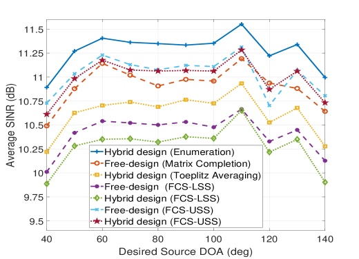
Figure 3: Average SINR performance of various sparse topologies against desired source DOA for $T=100$ snapshots.

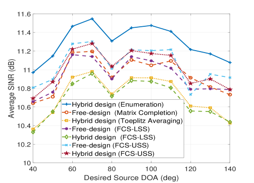
Figure 4: Average SINR performance of various sparse topologies against desired source DOA for $T=250$ snapshots.

The above examples tie the performance of the proposed algorithm not only to the location of the sources and their respective powers but also show the dependence on the initial array configuration, the number of snapshots and the observed realization of the received data. In order to provide a more meaningful assessment, the simulation scenarios are designed keeping the aforementioned variables in perspective. We generate $11$ different scenarios. For each scenario, the desired source DOA is kept fixed, whereas six jammers are randomly placed anywhere from $30^{0}$ to $150^{0}$ with the respective powers uniformly distributed from $5$ to $15$ dB. The experiments are repeated $3000$ times and the initial array configuration is randomly chosen for each experiment. For the freely designed array, the initial array configuration is selected by randomly choosing $16$ sensors from $36$ sensors. However, the initial configuration for the hybrid design is randomly chosen from all the possible $16$ sensor fully augmentable array configurations associated with the prefixed sensors arranged in nested configuration as depicted in Fig. 2(b) (red color sensors).

Figure 3 shows the results for $T=100$. The performance curve of the SCA algorithm for the freely designed array incorporating matrix completion lies in between (for most points) the benchmark designs incorporating FCM-USS and FCM-LSS. That is the matrix completion approach even outperforms the benchmark design incorporating the FCM-LSS. This performance is explainable because matrix completion coupled with the apriori knowledge of noise floor renders a more accurate estimate of the full correlation matrix as compared to FCM-LSS, without incorporating knowledge of noise floor, which has high noise variance because of limited snapshots. The performance of the other benchmark incorporating the exact knowledge of the correlation matrix (FCM-USS) is clearly superior over matrix completion. The results are fairly similar for the hybrid design, where the performance curve utilizing the Toeplitz averaging is sandwiched between the benchmark designs incorporating the exact correlation matrix (FCM-USS) and the one utilizing the presumably observed full data correlation matrix (FCM-LSS). The hybrid designed and freely designed arrays, both demonstrate desirable performances. However, the matrix completion marginally outperforms the hybrid design with an average performance gain of $0.2$ dB.

The performance curves are re-evaluated by increasing the snapshots to $T=250$ and $T=1000$, as shown in Figs. 4 and 5. With such increase, the performances of the proposed SCA using Toeplitz completion move closer to the performances of the FCM-USS benchmark. It is also noted that in contrast to lower snapshots ($T=100$), the FCM-LSS benchmark for higher samples ($T=1000$) offers superior average performance over SCA designs incorporating Toeplitz completion. It is of interest to track the average antenna switching involved per trial for both the free-design and the hybrid design. Fig. 6 shows that freely designed array involves $9$ antenna switching per trial which is more than twice that of the hybrid design ($4$ antenna switching per trial). It is also noted that for the hybrid design, the maximum antenna switching is constrained to $5$ antennas as the rest of $11$ sensors are prefixed. In this regard, the hybrid design has more efficient switching as it utilizes 80 percent (4/5) of the DOF as compared to the mere 55 percent (9/16) switching efficiency of freely designed arrays.

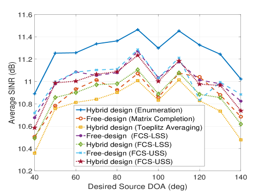
Figure 5: Average SINR performance of various sparse topologies against desired source DOA for $T=1000$ snapshots.

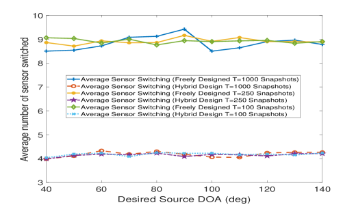
Figure 6: Sensor switching comparison vs the free-design and the hybrid design.

6 Conclusion

Sparse array design for maximizing the beamformer output SINR is considered for a single source in an interference active environment. The paper addressed the problem that the optimization of the array configuration requires full data correlation matrix which is not readily available in practice. Two different design approaches were considered; one assumes prefixed position of subset of sensors so as to provide full array augmentation, referred to as the hybrid-design approach, whereas the other, which is referred to as free-design approach, has no such restriction, and freely allocates all degrees of freedom to maximize the objective function. It was shown that the Toeplitz estimation of the autocorrelation at the missing spatial lags has a desirable performance. The SCA was proposed for both the freely designed and hybrid designed arrays to achieve MaxSINR in polynomial run times with a reasonable trade off in SINR. It was shown that, in contrast to hybrid design, the matrix completion scheme does not require to pre-allocate sensor resources and, therefore, offers more design flexibility and better SINR performance. This performance improvement is, however, at the cost of increased computational complexity and finer parameter tuning as required to accomplish Toepltiz matrix completion. The simulation examples provided showed that the performance of the proposed SCA algorithm incorporating Toeplitz completion is agreeable with the established benchmark designs.

References

- [1] G. R. Lockwood, J. R. Talman, S. S. Brunke, Real-time 3-D ultrasound imaging using sparse synthetic aperture beamforming, IEEE Transactions on Ultrasonics, Ferroelectrics, and Frequency Control 45 (4) (1998) 980–988. doi:10.1109/58.710573.
- [2] O. Mehanna, N. D. Sidiropoulos, G. B. Giannakis, Joint multicast beamforming and antenna selection, IEEE Transactions on Signal Processing 61 (10) (2013) 2660–2674.
- [3] W. V. Cappellen, S. J. Wijnholds, J. D. Bregman, Sparse antenna array configurations in large aperture synthesis radio telescopes, in: 2006 European Radar Conference, 2006, pp. 76–79. doi:10.1109/EURAD.2006.280277.
- [4] M. B. Hawes, W. Liu, Sparse array design for wideband beamforming with reduced complexity in tapped delay-lines, IEEE/ACM Transactions on Audio, Speech, and Language Processing 22 (8) (2014) 1236–1247. doi:10.1109/TASLP.2014.2327298.
- [5] S. Joshi, S. Boyd, Sensor selection via convex optimization, IEEE Transactions on Signal Processing 57 (2) (2009) 451–462. doi:10.1109/TSP.2008.2007095.
- [6] W. Roberts, L. Xu, J. Li, P. Stoica, Sparse antenna array design for MIMO active sensing applications, IEEE Transactions on Antennas and Propagation 59 (3) (2011) 846–858. doi:10.1109/TAP.2010.2103550.
- [7] H. Godrich, A. P. Petropulu, H. V. Poor, Sensor selection in distributed multiple-radar architectures for localization: A knapsack problem formulation, IEEE Transactions on Signal Processing 60 (1) (2012) 247–260. doi:10.1109/TSP.2011.2170170.
- [8] R. Rajamäki, V. Koivunen, Symmetric sparse linear array for active imaging, in: 2018 IEEE 10th Sensor Array and Multichannel Signal Processing Workshop (SAM), 2018, pp. 46–50. doi:10.1109/SAM.2018.8448767.
- [9] A. Moffet, Minimum-redundancy linear arrays, IEEE Transactions on Antennas and Propagation 16 (2) (1968) 172–175. doi:10.1109/TAP.1968.1139138.
- [10] P. Pal, P. P. Vaidyanathan, Nested arrays: A novel approach to array processing with enhanced degrees of freedom, IEEE Transactions on Signal Processing 58 (8) (2010) 4167–4181.
- [11] S. Qin, Y. D. Zhang, M. G. Amin, Generalized coprime array configurations for direction-of-arrival estimation, IEEE Transactions on Signal Processing 63 (6) (2015) 1377–1390.
- [12] E. BouDaher, Y. Jia, F. Ahmad, M. G. Amin, Multi-frequency co-prime arrays for high-resolution direction-of-arrival estimation, IEEE Transactions on Signal Processing 63 (14) (2015) 3797–3808. doi:10.1109/TSP.2015.2432734.
- [13] A. Ahmed, Y. D. Zhang, J. Zhang, Coprime array design with minimum lag redundancy, in: ICASSP 2019 - 2019 IEEE International Conference on Acoustics, Speech and Signal Processing (ICASSP), 2019, pp. 4125–4129. doi:10.1109/ICASSP.2019.8683315.
- [14] J. Li, P. Stoica, Z. Wang, On robust Capon beamforming and diagonal loading, IEEE Transactions on Signal Processing 51 (7) (2003) 1702–1715. doi:10.1109/TSP.2003.812831.
- [15] S. A. Hamza, M. G. Amin, G. Fabrizio, Optimum sparse array beamforming for general rank signal models, in: 2018 IEEE Radar Conference (RadarConf18), 2018, pp. 1343–1347. doi:10.1109/RADAR.2018.8378759.
- [16] S. A. Hamza, M. G. Amin, Sparse array DFT beamformers for wideband sources (2019). arXiv:1901.11474.
- [17] X. Wang, E. Aboutanios, M. Trinkle, M. G. Amin, Reconfigurable adaptive array beamforming by antenna selection, IEEE Transactions on Signal Processing 62 (9) (2014) 2385–2396.
- [18] N. D. Sidiropoulos, T. N. Davidson, Z.-Q. Luo, Transmit beamforming for physical-layer multicasting, IEEE Transactions on Signal Processing 54 (6) (2006) 2239–2251.
- [19] V. Roy, S. P. Chepuri, G. Leus, Sparsity-enforcing sensor selection for DOA estimation, in: 2013 5th IEEE International Workshop on Computational Advances in Multi-Sensor Adaptive Processing (CAMSAP), 2013, pp. 340–343.
- [20] X. Wang, M. Amin, X. Cao, Analysis and design of optimum sparse array configurations for adaptive beamforming, IEEE Transactions on Signal Processing PP (99) (2017) 1–1. doi:10.1109/TSP.2017.2760279.
- [21] X. Wang, M. G. Amin, X. Wang, X. Cao, Sparse array quiescent beamformer design combining adaptive and deterministic constraints, IEEE Transactions on Antennas and Propagation PP (99) (2017) 1–1.
- [22] X. Wang, M. Amin, Design of optimum sparse array for robust MVDR beamforming against DOA mismatch, in: 2017 IEEE 7th International Workshop on Computational Advances in Multi-Sensor Adaptive Processing (CAMSAP), 2017, pp. 1–5. doi:10.1109/CAMSAP.2017.8313065.
- [23] X. Wang, M. G. Amin, X. Cao, Optimum adaptive beamformer design with controlled quiescent pattern by antenna selection, in: 2017 IEEE Radar Conference (RadarConf), 2017, pp. 0749–0754.
- [24] S. Shahbazpanahi, A. B. Gershman, Z.-Q. Luo, K. M. Wong, Robust adaptive beamforming for general-rank signal models, IEEE Transactions on Signal Processing 51 (9) (2003) 2257–2269.
- [25] S. A. Hamza, M. G. Amin, Hybrid sparse array design for under-determined models, in: ICASSP 2019 - 2019 IEEE International Conference on Acoustics, Speech and Signal Processing (ICASSP), 2019, pp. 4180–4184. doi:10.1109/ICASSP.2019.8682266.
- [26] S. A. Hamza, M. G. Amin, Sparse array design utilizing matrix completion, in: 2019 Asilomar Conference on Signals, Systems, and Computers, 2019.
- [27] D. L. Donoho, For most large underdetermined systems of linear equations the minimal -norm solution is also the sparsest solution, Communications on Pure and Applied Mathematics 59 (6) 797–829.
- [28] M. S. Ibrahim, A. Konar, M. Hong, N. D. Sidiropoulos, Mirror-prox sca algorithm for multicast beamforming and antenna selection, in: 2018 IEEE 19th International Workshop on Signal Processing Advances in Wireless Communications (SPAWC), 2018, pp. 1–5. doi:10.1109/SPAWC.2018.8445845.
- [29] E. J. Candès, M. B. Wakin, S. P. Boyd, Enhancing sparsity by reweighted minimization, Journal of Fourier Analysis and Applications 14 (5) (2008) 877–905. doi:10.1007/s00041-008-9045-x.
- [30] B. Fuchs, Application of convex relaxation to array synthesis problems, IEEE Transactions on Antennas and Propagation 62 (2) (2014) 634–640. doi:10.1109/TAP.2013.2290797.
- [31] S. Eng Nai, W. Ser, Z. Liang Yu, H. Chen, Beampattern synthesis for linear and planar arrays with antenna selection by convex optimization 58 (2011) 3923 – 3930.
- [32] B. Recht, M. Fazel, P. A. Parrilo, Guaranteed minimum-rank solutions of linear matrix equations via nuclear norm minimization, SIAM Rev. 52 (3) (2010) 471–501. doi:10.1137/070697835.
- [33] K. Mohan, M. Fazel, Iterative reweighted algorithms for matrix rank minimization, J. Mach. Learn. Res. 13 (1) (2012) 3441–3473.
- [34] Z. q. Luo, W. k. Ma, A. M. c. So, Y. Ye, S. Zhang, Semidefinite relaxation of quadratic optimization problems, IEEE Signal Processing Magazine 27 (3) (2010) 20–34. doi:10.1109/MSP.2010.936019.
- [35] C. Zhou, Y. Gu, Z. Shi, Y. D. Zhang, Off-grid direction-of-arrival estimation using coprime array interpolation, IEEE Signal Processing Letters 25 (11) (2018) 1710–1714. doi:10.1109/LSP.2018.2872400.
- [36] C. Zhou, Y. Gu, X. Fan, Z. Shi, G. Mao, Y. D. Zhang, Direction-of-arrival estimation for coprime array via virtual array interpolation, IEEE Transactions on Signal Processing 66 (22) (2018) 5956–5971. doi:10.1109/TSP.2018.2872012.
- [37] C. Liu, P. P. Vaidyanathan, P. Pal, Coprime coarray interpolation for doa estimation via nuclear norm minimization, in: 2016 IEEE International Symposium on Circuits and Systems (ISCAS), 2016, pp. 2639–2642. doi:10.1109/ISCAS.2016.7539135.
- [38] S. M. Hosseini, M. A. Sebt, Array interpolation using covariance matrix completion of minimum-size virtual array, IEEE Signal Processing Letters 24 (7) (2017) 1063–1067. doi:10.1109/LSP.2017.2708750.
- [39] H. Qiao, P. Pal, Gridless line spectrum estimation and low-rank toeplitz matrix compression using structured samplers: A regularization-free approach, IEEE Transactions on Signal Processing 65 (9) (2017) 2221–2236. doi:10.1109/TSP.2017.2659644.
- [40] Y. I. Abramovich, D. A. Gray, A. Y. Gorokhov, N. K. Spencer, Positive-definite Toeplitz completion in DOA estimation for nonuniform linear antenna arrays. I. Fully augmentable arrays, IEEE Transactions on Signal Processing 46 (9) (1998) 2458–2471. doi:10.1109/78.709534.
- [41] Y. Abramovich, N. Spencer, A. Gorokhov, Positive-definite Toeplitz completion in DOA estimation for nonuniform linear antenna arrays. II. Partially augmentable arrays, Trans. Sig. Proc. 47 (6) (1999) 1502–1521.