Charging plug-in electric vehicles as a mixed-integer aggregative game

Abstract

We consider the charge scheduling coordination of a fleet of plug-in electric vehicles, developing a hybrid decision-making framework for efficient and profitable usage of the distribution grid. Each charging dynamics, affected by the aggregate behavior of the whole fleet, is modelled as an inter-dependent, mixed-logical-dynamical system. The coordination problem is formalized as a generalized mixed-integer aggregative potential game, and solved via semi-decentralized implementation of a sequential best-response algorithm that leads to an approximated equilibrium of the game.

I Introduction

Plug-in Electric Vehicles (PEVs) represent a promising alternative to the conventional fuel-based transportation [1]. However, they require a “smart” charge/discharge coordination to prevent undesired electricity demand peaks and congestion in the low-voltage distribution grid [2, 3]. Indeed, a fleet of PEVs can serve as a mobile extension of the grid, mitigating the intermittent behavior of renewable energy sources by storing (or providing) energy when the generation is higher (or lower) than the load demand. These capabilities are known as “ grid-to-vehicle” (g2v) and “vehicle-to-grid” (v2g), respectively [4]. In this context, a key role is played by the “fleet manager” or “aggregator”, which is partially responsible for providing charging services to the PEVs, coordinating the charge/discharge schedule to fulfill the needs of the PEVs owners and (desirably) providing ancillary services to the distribution system operator [1, 2].

Accordingly, an attracting framework that suitably condenses both individual interests and intrinsic limitations related with the shared facilities is represented by noncooperative game theory whose equilibrium solution, for instance in [5], allows to coordinate the charging of a population of PEVs in a decentralized fashion with the aim of filling the night-time valley. A similar non-cooperative equilibrium problem is addressed in [6] using mean field game theory, while in [7] the authors generalize the notion of valley-filling and study a social welfare optimization problem associated with the charging scheduling, proposing an asynchronous optimization algorithm. The PEV charging coordination game is further developed in [8] by including the battery degradation cost within the cost function of each vehicle. More generally, a semi-decentralized coordination algorithm based on fixed-point operator theory is proposed in [9], which achieves global exponential convergence to an aggregative equilibrium, even for large population size, while a distributed approach based on the progressive second price auction mechanism has been recently proposed in [10].

However, most of the models adopted in the literature do not describe the intrinsic discrete operations of each PEV, e.g., being plugged-in or plugged-out from one of the available charging points, in g2v or in v2g mode [11, 12, 13]. The selfish nature of each PEV, which pursues an economic, possibly profitable, usage of the charging station, together with the presence of both continuous (amount of energy charged/discharged) and discrete decision variables (operating mode) over a certain prediction horizon, motivates us to model the charge scheduling coordination of the PEVs as a collection of inter-dependent mixed-integer optimization problems, where the coupling constraints arise in aggregative form (§II). In fact, the common electricity price, as well as the operational limitations of the charging station, e.g., the number of charging points, directly depend on the overall behavior of the fleet. We then formulate the coordination problem as a mixed-integer aggregative game (§III), proving that it corresponds to a Mixed-Integer Generalized Potential Game (MI-GPG) [14]. Furthermore, we assume the presence of an aggregator, i.e., the charging station, that provides the aggregate information to the fleet and allows to compute an (approximated) equilibrium of the game by means of a semi-decentralized implementation of a sequential best-response algorithm (§IV). Finally, we define the game setup and the solution algorithm via numerical simulations on an illustrative scenario (§V).

Notation: $\mathbb{B}$ represents the binary set. For vectors $v_{1},\dots,v_{N}\in\mathbb{R}^{n}$ and $\mathcal{I}=\{1,\dots,N\}$, the collective strategy is denoted as $\boldsymbol{v}:=\mathrm{col}((v_{i})_{i\in\mathcal{I}})=[v_{1}^{\top},\dots,v_{N}^{\top}]^{\top}$ and $\boldsymbol{v}_{-i}:=\mathrm{col}((v_{j})_{j\in\mathcal{I}\setminus\{i\}})=[v_{1}^{\top},\dots,v_{i-1}^{\top},v_{i+1}^{\top},\dots,v_{N}^{\top}]^{\top}$. With a slight abuse of notation, we also use $\boldsymbol{v}=(v_{i},\boldsymbol{v}_{-i})$.

II PEVs scheduling and charge as a system of mixed-logical-dynamical systems

We start by modeling the charge scheduling of a PEV over a certain prediction horizon by first introducing the dynamics of the State of Charge (SoC) and the related control variables, both discrete and continuous. Then, we define the cost function that each PEV aims to minimize and, by means of logical implications, the interactions arising both among the set of PEVs itself and with the charging station.

II-A Decision variables and the SoC dynamics

Let $\mathcal{I}\coloneqq\{1,\dots,N\}$ be the set indexing a population of PEVs that share the charging resources on a single charging station with a finite number of charging points, over a prediction horizon $\mathcal{T}\coloneqq\{1,\dots,T\}$. For each vehicle $i\in\mathcal{I}$, the SoC of its battery at time $t\in\mathcal{T}$ is denoted by $x_{i}(t)\in[0,1]$, where $x_{i}(t)=1$ represents a fully charged battery, while $x_{i}(t)=0$ a completely discharged one. The amount of energy exchanged between each vehicle and the charging station, during the time period $t$, is denoted by $u_{i}(t)\in\mathcal{U}\coloneqq[\underline{u},\overline{u}]$, $\underline{u}<0$, $\overline{u}>0$. Specifically, $u_{i}(t)$ takes positive values if vehicle $i$ absorbs power during the time period $t$, while negative values if it gives energy back. For all $t\in\mathcal{T}$, we assume the dynamics of the SoC described by

$$x_{i}(t+1)=x_{i}(t)+b_{i}\delta_{i}(t)u_{i}(t)-(1-\delta_{i}(t))\mu_{i}(t),$$ (1)

where $b_{i}=\frac{\eta_{i}}{C_{i}}$ is a positive parameter which depends on the efficiency $\eta_{i}>0$ of the $i$-th battery and the corresponding capacity $C_{i}>0$. In (1), $\delta_{i}(t)\in\mathbb{B}$ is a scheduling variable of each vehicle, i.e., $\delta_{i}(t)=1$ if the $i$-th PEV is connected to the charging station at time $t$, $0$ otherwise. Within the dynamics (1), we consider that the SoC of the battery decreases when the vehicle is actively driving. In fact, if $\delta_{i}(t)=0$, the SoC decreases according to $\mu_{i}(t)>0$, which represents the discharge due to the energy consumed while driving during the time period $t\in\mathcal{T}$. Therefore, $\mu_{i}(t)>0$ (driving vehicle) can only affects the SoC when the PEV is not connected to the grid, i.e., $\delta_{i}(t)=0$. If the vehicle is not driving during the time period $t$, then $\mu_{i}(t)=0$.

Thus, over the whole horizon $\mathcal{T}$, each PEV $i\in\mathcal{I}$ has decision variables $u_{i}\coloneqq\mathrm{col}((u_{i}(t))_{t\in\mathcal{T}})$, $\delta_{i}\coloneqq\mathrm{col}((\delta_{i}(t))_{t\in\mathcal{T}})$ and controls the SoC, $x_{i}\coloneqq\mathrm{col}((x_{i}(t))_{t\in\mathcal{T}})$.

II-B Cost function

We assume that when the vehicle is connected to the charging station, it can either acquire energy from the charging station, or give it back. If the $i$-th PEV at time $t\in\mathcal{T}$ requires power from the charging station, i.e., $u_{i}>0$, then it faces a cost associated to the purchase and to the battery degradation. We model the first term as $c(d(t)+\sum_{j\in\mathcal{I}\setminus\{i\}}u_{j}^{+}(t))u_{i}(t)$, where we assume a fair electricity market with the cost per energy unit $c>0$, the same for all the PEVs, and $u_{j}^{+}(t)\coloneqq u_{j}(t)$ if $u_{j}(t)\geq 0$, $0$ otherwise. The values $(d(t))_{t\in\mathbb{N}}$ represent the non-PEV loads of the network, which is assumed to be a-priori known, while $\sum_{i\in\mathcal{I}\setminus\{i\}}u^{+}_{i}(t)\eqqcolon a_{i}(\boldsymbol{u}(t))$ is the aggregate demand of energy associated with the set of PEVs at time $t$. Then, we assume that the degradation cost associated to the charging of the battery is proportional to the variation of the energy exchanged between the PEV and the charging station, i.e., $\rho^{+}_{i}(u_{i}(t)-u_{i}(t-1))^{2}$, with $\rho^{+}_{i}>0$ depending on each single battery. Therefore, for all $t\in\mathcal{T}$ and for all $i\in\mathcal{I}$, the cost function associated to the charging phase (g2v) is

$$J^{\textup{g2v}}_{i}(u_{i}(t),\boldsymbol{u}_{-i}(t))\coloneqq c(d(t)+ a_{i}(\boldsymbol{u}(t)))u_{i}(t)$$

$$+\rho^{+}_{i}(u_{i}(t)-u_{i}(t-1))^{2}.$$

Similarly, when the PEV gives energy to the charging station, i.e., $u_{i}(t)<0$, the vehicle-to-grid (v2g) interaction implies a degradation cost due to the battery discharge, i.e., $\rho^{-}_{i}(u_{i}(t)-u_{i}(t-1))^{2}$, $\rho^{-}_{i}>0$. However, this cost is generally compensated by a reward $r_{i}(t)u_{i}(t)$, for some given values $(r_{i}(t))_{t\in\mathbb{N}}$, that the PEV receives from the charging station for actively participating in the scheduling. Thus, the cost function related with the v2g mode reads as

$$J^{\textup{v2g}}_{i}(u_{i}(t))\coloneqq r_{i}(t)u_{i}(t)+\rho^{-}_{i}(u_{i}(t)-u_{i}(t-1))^{2},$$

for all $t\in\mathcal{T}$ and $i\in\mathcal{I}$.

Now, we introduce two binary decision variables, i.e., $\delta^{\textup{c}}_{i}$, $\delta^{\textup{d}}_{i}\in\mathbb{B}$, which allow to model the mutual actions of charging/discharging and guarantee that the local cost function is equal to $0$ when $u_{i}=0$. They shall satisfy the next logical implications, for all $t\in\mathcal{T}$ and for all $i\in\mathcal{I}$:

$$[\delta^{\textup{c}}_{i}(t)=1]\iff[u_{i}(t)\geq 0],$$ (2)

$$[\delta^{\textup{d}}_{i}(t)=1]\iff[u_{i}(t)\leq 0].$$ (3)

Namely, $\delta^{\textup{c}}_{i}(t)$ (or, equivalently, $\delta^{\textup{d}}_{i}(t)$) is equal to $1$ if the PEV is not discharging (not charging), $0$ otherwise. Finally, for all $i\in\mathcal{I}$, the complete cost function reads as follows

$$J_{i}(u_{i},\delta^{\textup{d}}_{i},\delta^{\textup{c}}_{i},\boldsymbol{u}_{-i})\coloneqq\textstyle\sum_{t\in\mathcal{T}} J^{\textup{g2v}}_{i}(u_{i}(t),\boldsymbol{u}_{-i}(t))\left(1-\delta^{\textup{d}}_{i}(t)\right)$$ (4)

$$+J^{\textup{v2g}}_{i}(u_{i}(t))(1-\delta^{\textup{c}}_{i}(t)),$$

where $\delta^{\textup{c}}_{i}\coloneqq\mathrm{col}((\delta^{\textup{c}}_{i}(t))_{t\in\mathcal{T}})$ and $\delta^{\textup{d}}_{i}\coloneqq\mathrm{col}((\delta^{\textup{d}}_{i}(t))_{t\in\mathcal{T}})$.

II-C Local and global constraints

By considering a generic PEV $i\in\mathcal{I}$, first we assume that, for all $t\in\mathcal{T}$, it is desired that the corresponding level of SoC is at least equal to a reference level $x^{\textup{ref}}_{i}(t)\in[0,1]$, i.e.,

$$x^{\textup{ref}}_{i}(t)\leq x_{i}(t)\,.$$ (5)

The driving pattern of each PEV limits the possible values of $\delta_{i}(t)$. Namely, if $\mu_{i}(t)>0$ then feasible set of $\delta_{i}(t)$ is $\mathcal{B}(t)=0$; otherwise $\mathcal{B}(t)=\mathbb{B}$. Thus, this condition translate in a time varying feasible set $\mathcal{B}(t)$ of $\delta_{i}(t)$.

If $\delta_{i}(t)$ is left free, it may lead a vehicle to persistently switch between being connected and unconnected to the grid among consecutive time intervals. This behaviour is not only unnatural, but could also lead to a fast degradation of the battery [15]. To exclude this potential source of damage, we impose that, if a PEV is plugged-in at a certain time $t\in\mathcal{T}$, i.e., $\delta_{i}(t-1)=0$ and $\delta_{i}(t)=1$, then it has to remain connected to the charging station for at least $h_{i}\leq T,h_{i}\in\mathbb{N}$ consecutive time intervals. Thus, for all $i\in\mathcal{I}$ and $t\in\mathcal{T}$, this constraint can be rephrased via the logical implication

$$[\delta_{i}(t-1)=0]\wedge[\delta_{i}(t)=1]\Rightarrow[\delta_{i}(t+h)=1,\,\forall h\leq h_{i}].$$ (6)

Next, to exclude that a PEV charges or discharges when it is plugged-out (i.e., $\delta_{i}(t)=0$), we impose that $u_{i}(t)\in\mathcal{U}(t)\coloneqq[\underline{u}\delta_{i}(t),\overline{u}\delta_{i}(t)]$. Thus, $u_{i}(t)=0$ if $\delta_{i}(t)=0$, otherwise $u_{i}$ takes values in $[\underline{u},\overline{u}]$. Moreover, to exclude that a vehicle is plugged-in without being neither charged nor discharged, we impose that $\delta_{i}(t)=0$ if $u_{i}(t)=0$. Thus, the next logical implication needs to be satisfied for all $t\in\mathcal{T}$ and $i\in\mathcal{I}$:

$$[u_{i}(t)=0]\iff[\delta_{i}(t)=0].$$ (7)

Successively, due to the intrinsic limitations of the grid capacity $\overline{d}>0$, we assume that the amount of energy required in a single time period by both the PEVs and non-PEV loads cannot be greater than $\overline{d}$. This translates into a constraint on the PEVs total demand, i.e.,

$$d(t)+\textstyle\sum_{j\in\mathcal{I}}u_{j}(t)\in\left[0,\overline{d}\right].$$ (8)

Finally, it is natural to assume that the charging station has a finite number of charging spots, i.e., the number of vehicles that can charge/discharge at the same time cannot exceed a finite value $\overline{v}\in\mathbb{N}$. Thus, we impose, for all $t\in\mathcal{T}$,

$$\textstyle\sum_{j\in\mathcal{I}}\delta_{j}(t)\leq\overline{v}\>.$$ (9)

II-D Mixed-integer game formulation

We conclude this section by summarizing a preliminary formulation of the optimization problem for the scheduling and charging/discharging of each PEV as follows:

$$\forall i\in\mathcal{I}:\left\{\begin{aligned} &\underset{u_{i},x_{i},\delta_{i},\delta^{\textup{d}}_{i},\delta^{\textup{c}}_{i}}{\textrm{min}}&&J_{i}(u_{i},\delta^{\textup{d}}_{i},\delta^{\textup{c}}_{i},\boldsymbol{u}_{-i})\\ &\hskip 18.49411pt\textrm{s.t.}&&\eqref{eq:SoC_update_u},x_{i}(t)\in[0,1],\\ &&&u_{i}(t)\in\mathcal{U}(t),\delta_{i}(t)\in\mathcal{B}(t),\\ &&&\delta^{\textup{c}}_{i}(t),\delta^{\textup{d}}_{i}(t)\in\mathbb{B},\\ &&&\eqref{eq:logical_implication_deltar},\eqref{eq:logical_implication_sigma},\,\text{\eqref{eq:constraint_desiredlevel}--\eqref{eq:constraint_charging}},\;\forall t\in\mathcal{T}.\end{aligned}\right. \mathcal{G}$$ ()

We emphasize that several constraints in ($\mathcal{G}$), as well as the cost function, are either expressed as logical implications, or directly depend on the evaluation of a logical proposition. In the next section we translate all these logical implications into mixed-integer-linear inequalities, hence the problem in ($\mathcal{G}$) as a (parametric) mixed integer quadratic problem.

III Translating the logical implications into mixed-integer linear constraints

For the sake of clarity, we adopt the same notation used in [16, 17], i.e., we define several patterns of inequalities that allow to handle all the constraints. Specifically, given a linear function $f:\mathbb{R}\rightarrow\mathbb{R}$, let us define $M\coloneqq\textrm{max}_{x\in\mathcal{X}}f(x)$, $m\coloneqq\textrm{min}_{x\in\mathcal{X}}f(x)$ with $\mathcal{X}$ being a compact set. Then, with $c\in\mathbb{R}$ and $\delta\in\mathbb{B}$, a first system $\mathcal{S}_{\geq}$ of mixed-integer inequalities correspond to $[\delta=1]\iff[f(x)\geq c]$, i.e.,

$$\mathcal{S}_{\geq}(\delta,f(x),c)\coloneqq\left\{\begin{aligned} &(c-m)\delta\leq f(x)-m\\ &(M-c+\epsilon)\delta\geq f(x)-c+\epsilon,\end{aligned}\right.$$

Here $\epsilon>0$ is a small tolerance beyond which the constraint is regarded as violated. With the same idea, the following set of inequalities corresponds to $[\delta=1]\iff[f(x)\leq c]$:

$$\mathcal{S}_{\leq}(\delta,f(x),c)\coloneqq\left\{\begin{aligned} &(M-c)\delta\leq M-f(x)\\ &(c+\epsilon-m)\delta\geq\epsilon+c-f(x).\end{aligned}\right.$$

Successively, we define the next block of inequalities, involving binary variables only, which allow to solve propositions with logical AND, i.e., $[\delta=1]\iff[\sigma=1]\wedge[\gamma=1]$:

$$\mathcal{S}_{\wedge}(\delta,\sigma,\gamma)\coloneqq\left\{\begin{aligned} -&\sigma+\delta\leq 0\\ -&\gamma+\delta\leq 0\\ &\sigma+\gamma-\delta\leq 1,\end{aligned}\right.$$

Finally, to recast bilinear terms, i.e., products of binary and continuous variables, into a mixed-integer linear formulation, we introduce the following pattern of inequalities.

$$\mathcal{S}_{\Rightarrow}(g,f(x),\delta)\coloneqq\left\{\begin{aligned} &m\delta\leq g\leq M\delta\\ &-M(1-\delta)\leq g-f(x)\leq-m(1-\delta)\\ \end{aligned}\right.$$

The latter is equivalent to: $[\delta=0]\implies[g=0]$, while $[\delta=1]\implies[g=f(x)]$.

III-A The mixed-integer-linear constraints

The logical implications in (2) and (3) translate into:

$$\mathcal{S}_{\geq}(\delta^{\textup{c}}_{i}(t),u_{i}(t),0),$$ (10)

$$\mathcal{S}_{\leq}(\delta^{\textup{d}}_{i}(t),u_{i}(t),0).$$ (11)

By referring to the SoC dynamics in (1), the bilinear term $u_{i}\delta_{i}$ can be handled by following the procedure in [18], which allows to rewrite it as mixed-integer-linear inequalities by means of additional auxiliary variables (both real and binary, [19]). Specifically, we define the auxiliary variable $f_{i}\coloneqq u_{i}\delta_{i}\in\mathbb{R}$ that shall satisfy the pattern of inequalities:

$$\mathcal{S}_{\Rightarrow}(f_{i}(t),u_{i}(t),\delta_{i}(t)).$$ (12)

Thus, the SoC dynamics at the generic time $t\in\mathcal{T}$ reads as

$$x_{i}(t+1)=x_{i}(t)+b_{i}f_{i}(t)-(1-\delta_{i}(t))\mu_{i}(t),$$ (13)

The same approach allows to manage the bilinear terms that appear in the cost function (4). Hence, by defining $g_{i}(t)\coloneqq u_{i}(t)(1-\delta^{\textup{c}}_{i}(t))\in\mathbb{R}$, $s_{i}(t)\coloneqq u_{i}(t-1)(1-\delta^{\textup{c}}_{i}(t))\in\mathbb{R}$, $\ell_{i}(t)\coloneqq u_{i}(t)(1-\delta^{\textup{d}}_{i}(t))\in\mathbb{R}$ and $\kappa_{i}(t)\coloneqq u_{i}(t-1)(1-\delta^{\textup{d}}_{i}(t))\in\mathbb{R}$, subjected to inequalities, for all $i\in\mathcal{I}$ and $t\in\mathcal{T}$,

$$\mathcal{S}_{\Rightarrow}(g_{i}(t),u_{i}(t),1-\delta^{\textup{c}}_{i}(t)),$$ (14)

$$\mathcal{S}_{\Rightarrow}(s_{i}(t),u_{i}(t-1),1-\delta^{\textup{c}}_{i}(t)),$$ (15)

$$\mathcal{S}_{\Rightarrow}(\ell_{i}(t),u_{i}(t),1-\delta^{\textup{d}}_{i}(t)),$$ (16)

$$\mathcal{S}_{\Rightarrow}(\kappa_{i}(t),u_{i}(t-1),1-\delta^{\textup{d}}_{i}(t)),$$ (17)

the cost function (4) reads as (omitting the dependencies),

$$J_{i}=c (d(t)+a_{i}(\boldsymbol{u}(t)))\ell_{i}(t)+r_{i}(t)g_{i}(t)$$

$$+\rho_{i}^{-}\left(g_{i}(t)-s_{i}(t)\right)^{2}+\rho_{i}^{+}(\ell_{i}(t)-\kappa_{i}(t))^{2}\>.$$ (18)

Notice that via these variables we can rewrite also $a(\boldsymbol{u}(t))=\sum_{j\in\mathcal{I}\setminus\{i\}}\ell_{j}(t)$. Let us consider proposition (7), equivalently rewritten as $[u_{i}(t)\leq 0]\wedge[u_{i}(t)\geq 0]\implies[(1-\delta_{i}(t))=1].$ Since $\delta^{\textup{c}}_{i}$ and $\delta^{\textup{d}}_{i}$ already satisfy the inequalities in (10) and (11), for all $t\in\mathcal{T}$, the constraint in (7) reads as

$$\mathcal{S}_{\wedge}(1-\delta_{i}(t),\delta^{\textup{c}}_{i}(t),\delta^{\textup{d}}_{i}(t)).$$ (19)

Next, by referring to (6), we introduce a binary auxiliary variable $\alpha_{i}$, which is equal to $1$ when both $\delta_{i}(t-1)=0$ and $\delta_{i}(t)=1$, $0$ otherwise. Hence, $\alpha_{i}$ shall satisfy, for all $t\in\mathcal{T}$, $[\alpha_{i}(t)=1]\iff[(1-\delta_{i}(t-1))=1]\wedge[\delta_{i}(t)=1],$ which translates into the pattern of integer linear inequalities

$$\mathcal{S}_{\wedge}(\alpha_{i}(t),1-\delta_{i}(t-1),\delta_{i}(t)).$$ (20)

Thus, (6) can be rewritten as a nonlinear equality constraint $\alpha_{i}(t)\left(\sum_{h=1}^{h_{i}}\delta_{i}(t+h)-h_{i}\right)=0.$ Successively, we introduce a set of variables $\beta^{(h)}_{i}\in\mathbb{B}$ such that, for all $t\in\mathcal{T}$, $[\beta^{(h)}_{i}(t)=1]\iff[\alpha_{i}(t)=1]\wedge[\delta_{i}(t+h)=1,\,\forall h\leq h_{i}],$ which corresponds to the following patterns of inequalities

$$\mathcal{S}_{\wedge}(\beta^{(h)}_{i}(t),\alpha_{i}(t),\delta_{i}(t+h)),\;\forall h\leq h_{i}.$$ (21)

This allows to rewrite the equality constraint in linear form

$$\textstyle{\sum_{h=1}^{h_{i}}}\beta^{(h)}_{i}(t)-\alpha_{i}(t)h_{i}=0.$$ (22)

III-B Final mixed-integer-linear model

By rearranging all the inequalities, we obtain the following mixed-integer aggregative game

$$\forall i\in\mathcal{I}:\left\{\begin{aligned} &\underset{u_{i},x_{i},\ldots,\beta_{i}}{\textrm{min}}&&J_{i}(u_{i},g_{i},s_{i},\ell_{i},\kappa_{i},\boldsymbol{u}_{-i})\\ &\hskip 14.22636pt\textrm{s.t.}&&\eqref{eq:constraint_desiredlevel},x_{i}(t)\in[0,1],\\ &&&\text{\eqref{eq:constraint_totalamount}--\eqref{eq:third_MI}},\text{\eqref{eq:bau}--\eqref{eq:sixth_MI}},\\ &&&u_{i}(t),f_{i}(t),g_{i}(t),s_{i}(t)\in\mathcal{U}(t),\\ &&&\ell_{i}(t),\kappa_{i}(t)\in\mathcal{U}(t),\;\delta_{i}(t)\in\mathcal{B}(t),\\ &&&\delta^{\textup{c}}_{i}(t),\alpha_{i}(t),\delta^{\textup{d}}_{i}(t)\in\mathbb{B},\;\forall t\in\mathcal{T},\\ &&&\beta^{(h)}_{i}(t)\in\mathbb{B},\;\forall h\leq h_{i},\forall t\in\mathcal{T}.\end{aligned}\right.$$ (23)

The coupling constraints in (8)–(9), as well as the cost function, depend on the aggregate behavior of the fleet of PEVs. By defining $z_{i}\coloneqq\mathrm{col}(u_{i},x_{i},\ldots,\beta_{i})\in\mathbb{R}^{n_{i}}$ and $\boldsymbol{z}\coloneqq\mathrm{col}((z_{i})_{i\in\mathcal{I}})\in\mathbb{R}^{n}$, $n\coloneqq\sum_{i\in\mathcal{I}}n_{i}$, as the vectors stacking local and collective mixed-integer variables, respectively, we have, for some suitable matrix $A$ and vector $b$,

$$\forall i\in\mathcal{I}:\underset{z_{i}}{\textrm{min}}\;J_{i}(z_{i},\boldsymbol{z}_{-i})\;\;\textrm{s.t. }\;A\boldsymbol{z}\leq b.$$ (24)

IV PEVs charge coordination as a generalized mixed-integer potential game

Our aim is now to design suitable sequences of decisions that guarantee to each PEV an effective, economic, possibly profitable, usage of the electrical distribution network, while satisfying both the intrinsic limitations of the charging station itself, and by the presence of the other vehicles. We propose to achieve such a trade-off by formalizing the charge coordination of the set of PEVs as a MI-GPG [14], an instance of the Generalized Nash Equilibrium Problems (GNEPs) [20].

IV-A Potential game setup

First, we identify the player set with $\mathcal{I}$, and we define the feasible set of each player, i.e., $\mathcal{Z}_{i}(\boldsymbol{z}_{-i})\coloneqq\{z_{i}\in\mathbb{R}^{n_{i}}\mid A(z_{i},\boldsymbol{z}_{-i})\leq b\}$, and $\boldsymbol{\mathcal{Z}}\coloneqq\{\boldsymbol{z}\in\mathbb{R}^{n}\mid A\boldsymbol{z}\leq b\}$. Next, we introduce the mixed-integer best response mapping for player $i$, given the strategies of the other players $\boldsymbol{z}_{-i}$:

$$z^{\star}_{i}(\boldsymbol{z}_{-i})\coloneqq\underset{z_{i}}{\textrm{argmin}}\;J_{i}(z_{i},\boldsymbol{z}_{-i})\;\;\textrm{s.t. }\;(z_{i},\boldsymbol{z}_{-i})\in\boldsymbol{\mathcal{Z}}.$$ (25)

Hence, in the proposed game $\Gamma\coloneqq\left(\mathcal{I},\{J_{i}\}_{i\in\mathcal{I}},\{\mathcal{Z}_{i}\}_{i\in\mathcal{I}}\right)$, we are interested in the following notion of equilibrium.

Definition 1 ($\varepsilon$-Mixed-Integer Nash equilibrium)

Let $\varepsilon>0$. $\boldsymbol{z}^{*}\in\boldsymbol{\mathcal{Z}}$ is an $\varepsilon$-Mixed-Integer Nash Equilibrium ($\varepsilon$-MINE) of the game $\Gamma$ in (25) if, for all $i\in\mathcal{I}$,

$$J_{i}(z^{*}_{i},\boldsymbol{z}^{*}_{-i})\leq\underset{z_{i}\in\mathcal{Z}_{i}(\boldsymbol{z}^{*}_{-i})}{\textrm{inf}}J_{i}(z_{i},\boldsymbol{z}^{*}_{-i})+\varepsilon.$$

$\square$

We consider here potential games characterized by the existence of an exact potential function, defined next.

Definition 2

A continuous function $P:\mathbb{R}^{n}\to\mathbb{R}$ is an exact potential function for the game $\Gamma$ in (25) if, for all $i\in\mathcal{I}$, for all $\boldsymbol{z}_{-i}$, and for all $z_{i}$, $y_{i}\in\mathcal{Z}_{i}(\boldsymbol{z}_{-i})$,

$$P(z_{i},\boldsymbol{z}_{-i})-P(y_{i},\boldsymbol{z}_{-i})=J_{i}(z_{i},\boldsymbol{z}_{-i})-J_{i}(y_{i},\boldsymbol{z}_{-i}).\quad\square$$

Now, let us consider the cost function in (III-A) defined for all $t\in\mathcal{T}$. Due to the particular structure of the cost of the acquired energy, in compact form it reads as

$$J_{i}(z_{i},\boldsymbol{z}_{-i})=\phi_{i}(z_{i})+\textstyle\sum_{j\in\mathcal{I}\setminus\{i\}}\omega_{ij}(z_{i},z_{j}),$$ (26)

where $\phi_{i}(z_{i})\coloneqq z_{i}^{\top}Q_{i}z_{i}+q_{i}^{\top}z_{i}$, for some suitable positive semi-definite matrix $Q_{i}\in\mathbb{R}^{n_{i}\times n_{i}}$ and vector $q_{i}\in\mathbb{R}^{n_{i}}$, while

$$\omega_{ij}(z_{i},z_{j})\coloneqq z_{j}^{\top}\left[\begin{smallmatrix}\boldsymbol{0}&\boldsymbol{0}&\boldsymbol{0}\\ \boldsymbol{0}&c\,I&\boldsymbol{0}\\ \boldsymbol{0}&\boldsymbol{0}&\boldsymbol{0}\end{smallmatrix}\right]z_{i}=c\,\ell_{j}^{\top}\ell_{i}.$$

Theorem 1

The game $\Gamma$ in (25) is an MI-GPG with exact potential function

$$P(\boldsymbol{z})\coloneqq\textstyle\sum_{i\in\mathcal{I}}\left(\phi_{i}(z_{i})+\textstyle\sum\limits_{j\in\mathcal{I},j<i}\omega_{ij}(z_{i},z_{j})\right).$$ (27)

$\square$

Proof:

The proof replicates the one in [21, Prop. 2]. ∎

To conclude, we recall that the set of $\varepsilon$-approximated minimum over $\boldsymbol{\mathcal{Z}}$ of $P$ corresponds to a subset of the $\varepsilon$-MINE of the game [22, Th. 2].

IV-B Semi-decentralized solution algorithm

Initialization: Choose $\boldsymbol{z}(0)\in\boldsymbol{\mathcal{Z}}$, set $k\coloneqq 0$

while $\boldsymbol{z}(k)$ is not an $\varepsilon$-MINE do

       $\mathcal{AG}$ do

             Chooses $i\coloneqq i(k)\in\mathcal{I}$

             Sets $p_{i}(\boldsymbol{u}(k))$ as in (28), $e(\boldsymbol{\delta}(k))$ as in (29)

             Sends $p_{i}(\boldsymbol{u}(k))$, $e(\boldsymbol{\delta}(k))$ to $i$

      end 

      Player $i$ do

             Compute $z^{\ast}_{i}(k)\in z^{\star}_{i}(k)$ as in (25)

             if $J_{i}(z_{i}(k),p_{i}(\boldsymbol{u}(k)))-J_{i}(z_{i}^{\ast}(k),p_{i}(\boldsymbol{u}(k)))\geq\varepsilon$ 

                   $z_{i}(k+1)\coloneqq z^{\ast}_{i}(k)$

             else

                   $z_{i}(k+1)\coloneqq z_{i}(k)$

             end if

            

      end 

      $\mathcal{AG}$ collects $z_{i}(k+1)$

       Set $z_{j}(k+1)\coloneqq z_{j}(k)\;\forall j\neq i$, $k\coloneqq k+1$

end while

Algorithm 1 Sequential best-response

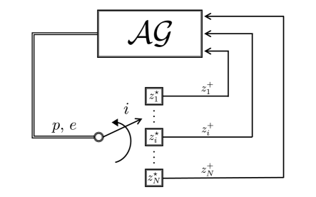
Figure 1: Semi-decentralized implementation of Algorithm 1, where $z_{i}^{+}\coloneqq z_{i}(k+1)$.

To compute a solution to (24), each player requires the aggregate information over the whole horizon $\mathcal{T}$, i.e., the PEVs demand of energy $a_{i}(\boldsymbol{u})\coloneqq\mathrm{col}((a_{i}(\boldsymbol{u}(t)))_{t\in\mathcal{T}})$, or, equivalently, the price associated to such demand

$$p_{i}(\boldsymbol{u})\coloneqq c(d+a_{i}(\boldsymbol{u})),$$ (28)

with $d\coloneqq\mathrm{col}((d(t))_{t\in\mathcal{T}})$, and the number of available charging points at the charging station, i.e.,

$$e(\boldsymbol{\delta})\coloneqq\overline{v}\boldsymbol{1}_{T}-\left(\boldsymbol{1}_{N}^{\top}\otimes I_{T}\right)\boldsymbol{\delta},$$ (29)

where $\boldsymbol{\delta}\coloneqq\mathrm{col}((\delta_{i})_{i\in\mathcal{I}})$. Specifically, while the number of available charging points $e(\boldsymbol{\delta})$ reflects the coupling constraint in (9), the price of energy $p_{i}(\boldsymbol{u})$ affects both the constraints and the cost function in (26), which can be equivalently expressed as function of $z_{i}$ and $p_{i}(\boldsymbol{u})$.

In this context, it seems unrealistic or, at least, impractical to assume full communication among all the potential users of the same charging station, over the same horizon $\mathcal{T}$. Therefore, to compute an $\varepsilon$-MINE, we propose a semi-decentralized implementation of the sequential best-response method, summarized in Algorithm 1, that includes an aggregator $\mathcal{AG}$, whose role is played by the charging station, within the communication pattern. According to [1], we assume the driving patterns of each PEV to be known by the $\mathcal{AG}$. As shown in the scheme in Fig. 1, at each iteration $k$, the aggregator $\mathcal{AG}$ chooses the next agent taking part in the game, communicating the price of energy and the number of available charging points. With this information, the selected agent computes a best response and decides to change strategy only if it leads to an (at least) $\varepsilon$-improvement in terms of minimization of its cost function. Finally, $\mathcal{AG}$ collects the decision of such agent, while the remaining part of players keeps its strategy unchanged.

Corollary 1

Let $\varepsilon>0$ and assume that, in Algorithm 1, there exists $K>0$ such that $j\in\{i(k),i(k+1),\ldots,i(k+K)\}$ for all $j\in\mathcal{I}$ and $k\geq 0$. Algorithm 1 computes an $\varepsilon$-MINE, $\boldsymbol{z}^{\ast}\in\boldsymbol{\mathcal{Z}}$, of the game $\Gamma$ in (25). $\square$

Proof:

In view of Theorem 1, the game $\Gamma$ in (25) is an MI-GPG. Therefore, by [22, Th. 4], the sequential best-response based Algorithm 1 converges to an $\varepsilon$-MINE. ∎

V Numerical simulations

In this section, we show numerical results obtained by solving the MI-GPG in (25) with parameter values specified in Tab. I (see [5, 13, 23]) and reward function $r(t)$ chosen proportional to the nominal demand and the energy generated by the vehicles, i.e., $r(t)\coloneqq\overline{r}(\sum_{j\in\mathcal{I}\setminus\{i\}}u^{-}_{j}(t)+d(t))$, where $d(t)$ corresponds to a typical daily demand curve [13], and $u^{-}_{j}(t)$ defined analogously to $u^{+}_{j}(t)$.

TABLE I: Simulation parameters

Name	[ ]	Description	Values
$N$		PEVs number	$6$
$T$		Time intervals in $24h$	$48$
$u$	[kWh]	Energy exchanged per interval	$[-7.5,7.5]$
$\eta$		Battery efficiency	$0.85$
$C_{i}$	[kWh]	Battery capacity	$[40,75]$
$x_{0}$		Initial SoC of battery	$0.23$
$x^{\mathrm{ref}}$		Ref. battery SoC	$[0.2,0.85]$
$c$	[€/kWh]	Energy cost	$1.09\times 10^{-3}$
$\bar{r}$	[€/kWh]	Constant reward	$1.23\times 10^{-3}$
$\rho^{+}\,(\rho^{-})$	[€/kWh2]	Degradation cost	$1(0.5)\times 10^{-3}$
$\overline{d}$	[kWh]	Grid power capacity	$45$
$h$		Min. consecutive v2g slots	$5$
$\overline{v}$		Max. connected PEVs	$5$

For a subset of PEVs, we show in Fig. 2 that the SoC $x_{i}(t)$, as well as the scheduling variable $\delta_{i}(t)$, satisfy the constraints on the required SoC $x_{i}^{\mathrm{ref}}(t)$ (5) and on the number $h_{i}$ of plugged-in consecutive intervals (6).

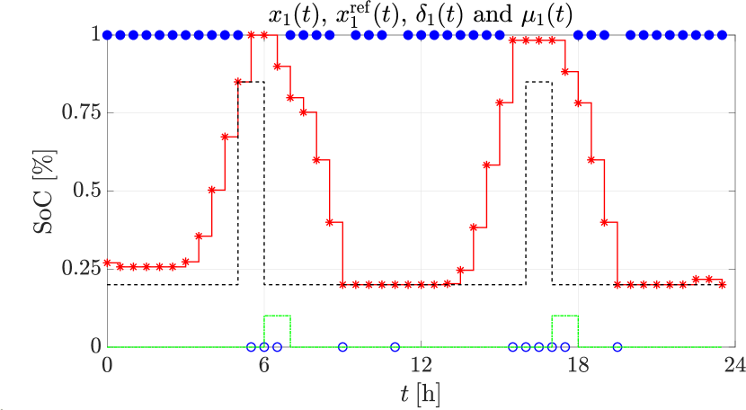
(a)

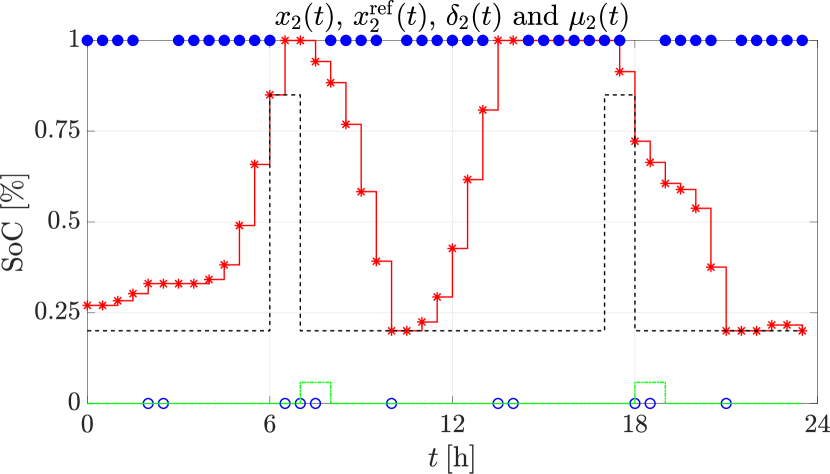
(b)

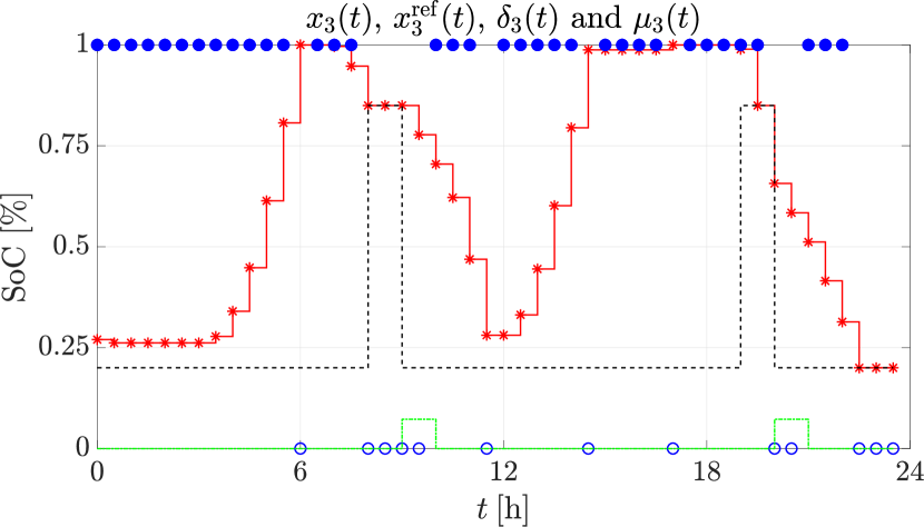
(c)

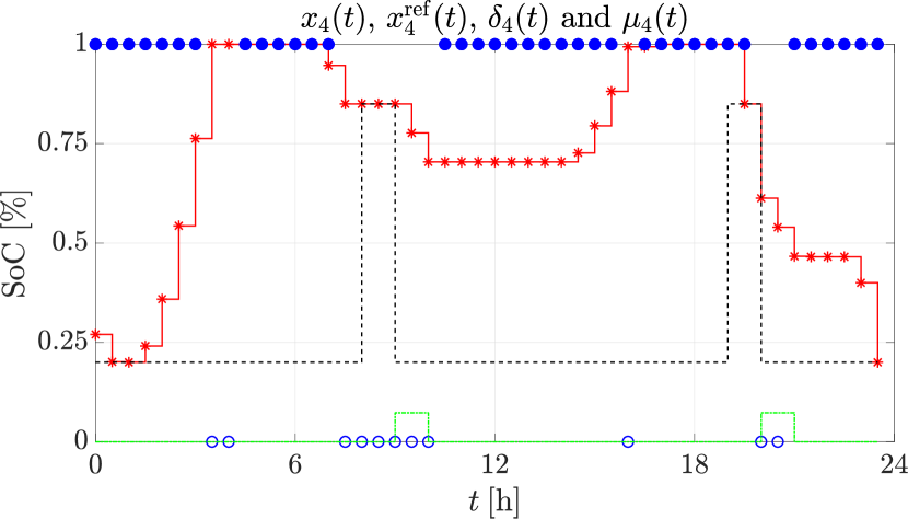
(d)

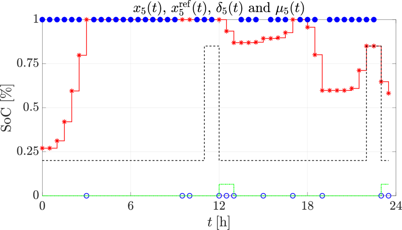
(e)

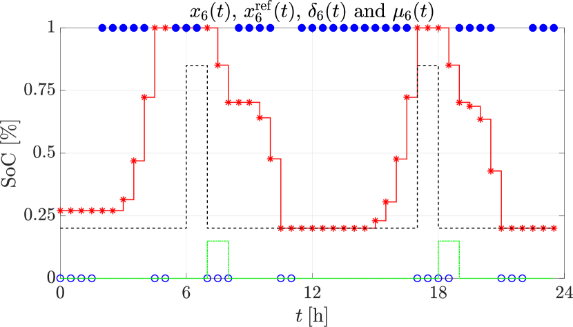
(f)

Figure 2: For each PEV $i\in\mathcal{I}$, the SoC $x_{i}(t)$ (solid red line), the desired lower bound of the SoC $x_{i}^{\mathrm{ref}}(t)$ (dashed black line), the value of the binary sheduling variable $\delta_{i}(t)$ (empty and filled blue circles) and $\mu_{i}(t)$ (dashed green line), over the horizon $\mathcal{T}$.

In Fig. 3, note that the peak value of $d(t)$ exceeds the maximum capacity $\overline{d}$ at $t=$ 19 h. Consequently, the constraint (8) forces some of the vehicles to discharge during this time period, showing the so-called “valley filling” phenomenon.

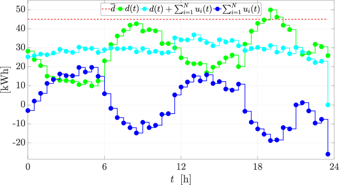
Figure 3: Power required by the load in the grid $d(t)$ (green), the one exchanged with the fleet, $\sum_{i=1}^{N}u_{i}(t)$ (blue) and the maximum capacity of the charging station, $\overline{d}$ (red dashed).

Finally, Fig. 4 shows the value of the potential function $P(\boldsymbol{z})$ and the convergence of the algorithm after approximately $25$ iterations.

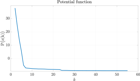
Figure 4: The values of the potential function $P(\boldsymbol{z})$ associated to the updating PEV in Algorithm 1.

VI Conclusion and outlook

A mixed-integer aggregative game can efficiently solve the charge scheduling coordination of a fleet of PEVs, each one modeled as a system of mixed-logical-dynamical systems. Discrete decision variables, as well as logical propositions, allow to catch the different interests of each PEV and the heterogeneous interactions between both the set of vehicles itself and the charging station. By playing the role of central aggregator, the charging station is key in computing an (approximated) equilibrium of the associated generalized potential game in a semi-decentralized fashion. In fact, the specific sequence of activation of the PEVs highly influences both the outcome of the game and the speed of convergence. The analysis of this phenomenon is left to future works, as well as the generalization in the case of multiple charging stations, i.e., possible multiple central aggregators.

References

• [1] J. Hu, H. Morais, T. Sousa, and M. Lind, “Electric vehicle fleet management in smart grids: A review of services, optimization and control aspects,” Renewable and Sustainable Energy Reviews, vol. 56, pp. 1207–1226, 2016.
• [2] R. J. Bessa and M. A. Matos, “Economic and technical management of an aggregation agent for electric vehicles: A literature survey,” European Transactions on Electrical Power, vol. 22, no. 3, pp. 334–350, 2012.
• [3] K. Clement-Nyns, E. Haesen, and J. Driesen, “The impact of charging plug-in hybrid electric vehicles on a residential distribution grid,” IEEE Transactions on Power Systems, vol. 25, no. 1, pp. 371–380, 2010.
• [4] E. Sortomme and M. A. El-Sharkawi, “Optimal scheduling of vehicle-to-grid energy and ancillary services,” IEEE Transactions on Smart Grid, vol. 3, no. 1, pp. 351–359, 2012.
• [5] Z. Ma, D. S. Callaway, and I. A. Hiskens, “Decentralized charging control of large populations of plug-in electric vehicles,” IEEE Transactions on Control Systems Technology, vol. 21, no. 1, pp. 67–78, 2013.
• [6] F. Parise, M. Colombino, S. Grammatico, and J. Lygeros, “Mean field constrained charging policy for large populations of plug-in electric vehicles,” in 53rd IEEE Conference on Decision and Control, 2014, pp. 5101–5106.
• [7] L. Gan, U. Topcu, and S. H. Low, “Optimal decentralized protocol for electric vehicle charging,” IEEE Transactions on Power Systems, vol. 28, no. 2, pp. 940–951, 2013.
• [8] Z. Ma, S. Zou, L. Ran, X. Shi, and I. A. Hiskens, “Efficient decentralized coordination of large-scale plug-in electric vehicle charging,” Automatica, vol. 69, pp. 35–47, 2016.
• [9] S. Grammatico, “Exponentially convergent decentralized charging control for large populations of plug-in electric vehicles,” in 2016 IEEE 55th Conference on Decision and Control (CDC), 2016, pp. 5775–5780.
• [10] S. Zou, Z. Ma, X. Liu, and I. Hiskens, “An efficient game for coordinating electric vehicle charging,” IEEE Transactions on Automatic Control, vol. 62, no. 5, pp. 2374–2389, 2017.
• [11] P. You, Z. Yang, M. Chow, and Y. Sun, “Optimal cooperative charging strategy for a smart charging station of electric vehicles,” IEEE Transactions on Power Systems, vol. 31, no. 4, pp. 2946–2956, 2016.
• [12] H. Xing, M. Fu, Z. Lin, and Y. Mou, “Decentralized optimal scheduling for charging and discharging of plug-in electric vehicles in smart grids,” IEEE Transactions on Power Systems, vol. 31, no. 5, pp. 4118–4127, 2016.
• [13] J. Rivera, C. Goebel, and H. Jacobsen, “Distributed convex optimization for electric vehicle aggregators,” IEEE Transactions on Smart Grid, vol. 8, no. 4, pp. 1852–1863, 2017.
• [14] F. Facchinei, V. Piccialli, and M. Sciandrone, “Decomposition algorithms for generalized potential games,” Computational Optimization and Applications, vol. 50, no. 2, pp. 237–262, 2011.
• [15] A. Millner, “Modeling lithium ion battery degradation in electric vehicles,” in 2010 IEEE Conference on Innovative Technologies for an Efficient and Reliable Electricity Supply, 2010, pp. 349–356.
• [16] F. Fabiani and S. Grammatico, “A mixed-logical-dynamical model for automated driving on highways,” in 2018 IEEE Conference on Decision and Control (CDC).   IEEE, 2018, pp. 1011–1015.
• [17] ——, “Multi-vehicle automated driving as a generalized mixed-integer potential game,” IEEE Transactions on Intelligent Transportation Systems, 2019, (In press).
• [18] A. Bemporad and M. Morari, “Control of systems integrating logic, dynamics, and constraints,” Automatica, vol. 35, no. 3, pp. 407–427, 1999.
• [19] H. P. Williams, Model building in Mathematical Programming.   John Wiley & Sons, 2013.
• [20] F. Facchinei and C. Kanzow, “Generalized Nash equilibrium problems,” 4OR: A Quarterly Journal of Operations Research, vol. 5, no. 3, pp. 173–210, 2007.
• [21] F. Fabiani and A. Caiti, “Nash equilibrium seeking in potential games with double-integrator agents,” in 2019 18th European Control Conference (ECC).   IEEE, 2019, pp. 548–553.
• [22] S. Sagratella, “Algorithms for generalized potential games with mixed-integer variables,” Computational Optimization and Applications, pp. 1–29, 2017.
• [23] M. de Vent, “Distributed optimal control of smart electricity grids: Home battery and electric vehicle implementation,” 2018. [Online]. Available: http://fse.studenttheses.ub.rug.nl/18698/