One Dimensional Localization for Arbitrary Disorder Correlations

Abstract

We evaluate the localization length of the wave solution of a random potential characterized by an arbitrary autocorrelation function. We go beyond the Born approximation to evaluate the localization length using a non-linear approximation and calculate all the correlators needed for the localization length expression. We compare our results with numerical results for the special case, where the autocorrelation decays quadratically with distance. We look at disorder ranging from weak to strong disorder, which shows excellent agreement. For the numerical simulation, we introduce a generic method to obtain a random potential with an arbitrary autocorrelation function. The correlated potential is obtained in terms of the convolution between a Wiener stochastic potential and a function of the correlation.

1 Introduction

Disordered systems are playing an important role in materials physics Cutler and Mott (1969); Thouless (1979); Berthier and Biroli (2011), cold atoms Billy et al. (2008); Roati et al. (2008), optical waveguides Elson et al. (1983); John (1987); Topolancik et al. (2007); Hilke (2009); Karbasi et al. (2014); Skipetrov (2014), acoustic and phononic systems Weaver (1990), many-body systems Basko et al. (2006); Bardarson et al. (2012) and even time fluctuations Fishman et al. (1982); Brandenberger and Craig (2012). While in some cases physical properties depend on a particular disorder configuration, most properties depend on their configurational average Hilke (2008). A good example being the resistance through a macroscopic disordered system. If the system size is much greater than the coherence length, the resistance can be computed by doing a configurational average Huckestein (1995). In this case only the statistical properties of the disorder are important, particularly the autocorrelator. There has been a long history of important results based on the assumption of uncorrelated disorder (or white disorder), in particular, the seminal result by Anderson Anderson (1958) on the localization of all states in one dimension Thouless (1979); Abrahams et al. (1979); Kunz and Souillard (1980). In general, the solution to a problem with disorder is challenging, yet the assumption of uncorrelated disorder greatly simplifies the evaluation of averaged properties Pendry (1994). However, in many physical systems, uncorrelated disorder is not a valid assumption, like for instance in speckle potentials Cao (2003); Sanchez-Palencia et al. (2007); Hilke and Eleuch (2017) or smooth random potentials de Moura and Lyra (1998); Izrailev and Krokhin (1999); Shima et al. (2004); Izrailev et al. (2012); Eleuch and Hilke (2015). In fact, correlations in the disorder can lead to delocalization in 1D Erdös and Herndon (1982); Flores (1989); Dunlap et al. (1990); Flores and Hilke (1993); Sánchez et al. (1994); Hilke and Flores (1997); Bellani et al. (1999) and 2D Hilke (1994, 2003). Hence finding tools to address systems where the disorder is not just uncorrelated but defined by some correlation function is crucial.

In some cases it is possible to use the Born approximation in order to find the disorder averaged properties, such as localization. This approach works well when coherent multiple scattering is neglected, which is often the case for weak disorder. Properties such as the mean free path or localization then simply depend on the Fourier transform of the disorder potential. For more general disorder potentials other methods have to be used, such as perturbation expansion Sánchez et al. (1994); Tessieri (2002) or phase averaging. Here we discuss another method, which is based on finding the exact solution of a non-linear extension of the wave equation Eleuch et al. (2010); Eleuch and Hilke (2015).

2 Non-linear approximation to the wave equation equation in a random potential

The 1D wave equation (or Schrödinger equation with $\hbar=2m=1$) is given by

$$[\partial_{x}^{2}+p(x)^{2}]\psi(x)=0,$$ (1)

with classical momentum

$$p(x)\equiv\partial_{x}P(x)=\sqrt{V(x)-E},$$ (2)

where we have defined $P(x)$ as the integrated momentum.

When looking for a solution of the form

$$\psi(x)=e^{i(P+N)}=e^{i\int_{0}^{x}f(x^{\prime})dx^{\prime}},$$ (3)

normalized at $x=0$, we obtain the following non-linear equation for $N(x)$

$$i(\partial_{x}N)^{2}+2ip\partial_{x}N+\partial_{x}p+\partial_{x}^{2}N=0,$$ (4)

which is difficult to solve Eleuch et al. (2010); Eleuch and Rostovtsev (2010). So instead, we can solve the related non-linear wave equation

$$[\partial_{x}^{2}+p^{2}-[\psi^{-1}(-i\partial_{x}-p)\psi]^{2}]\psi=0,$$ (5)

which leads to a linear equation in $N(x)$:

$$2ip\partial_{x}N+\partial_{x}p+\partial_{x}^{2}N=0$$ (6)

using equ. (3). This is equivalent to assuming $(\partial_{x}N)^{2}=0$ in equ. (4). The non-linear approximation corresponds to neglecting the difference between the classical and quantum momentum to second order: $((p+i\partial_{x})\psi)^{2}\simeq 0$. The differential operator corresponding to equ. (6) is then

$$H_{N} = 2ip\partial_{x}+\partial_{x}^{2}$$ (7)

$$= e^{-2iP}\partial_{x}(e^{2iP}\partial_{x}),$$

where we need to solve

$$H_{N}N=-\partial_{x}p.$$ (8)

The solution can be obtained by integration, i.e.,

$$\partial_{x}N(x)=-e^{-2iP(x)}\int^{x}e^{2iP(x^{\prime})}k^{\prime}_{v}(x^{\prime})dx^{\prime}\\$$

to give

$$f(x)=p(x)-e^{-2iP(x)}\int^{x}e^{2iP(x^{\prime})}p^{\prime}(x^{\prime})dx^{\prime}.\\$$

The average over disorder can be performed, which gives

$$\langle f(x)\rangle=\langle p(x)\rangle-\int_{0}^{x}e^{-2ik_{0}x^{\prime}}c_{p}(x^{\prime}),$$ (9)

where

$$c_{p}(x)=\langle k^{\prime}(0)e^{-2iP(x)}\rangle$$ (10)

is the correlation function of the disorder potential, where we defined the average momentum $k_{0}=\langle p(x)\rangle$), the variation from the mean ($k(x)=p(x)-k_{0}$) and its spatial derivative ($k^{\prime}(x)$). To obtain (9) one has to assume that the disorder is translationally uniform. The decay of the wave solution (Lyapounov exponent, $\lambda$ or inverse localization length) is then given by Eleuch and Hilke (2015); Hilke and Eleuch (2017)

$$\lambda=\Im\langle f(x)\rangle,$$ (11)

which can be rewritten as

$$\lambda=-2\Re\left\{\int_{0}^{\infty}\left(k_{0}C_{1}(x)+C_{2}\left(x\right)\right)e^{-2ik_{0}x}dx\right\},$$ (12)

where

$$C_{n}(x)=\left\langle k(0)^{n}e^{-2iP(x)}\right\rangle.$$ (13)

This equation was shown to be valid for all disorder strengths for a number of disorder correlations, such as Gaussian Eleuch and Hilke (2015), speckle Hilke and Eleuch (2017) and square well potentials Eleuch and Hilke (2018). In the limit of weak disorder the well known Born approximation is retrieved Izrailev et al. (2012); Eleuch and Hilke (2015):

$$\lambda_{\tilde{V}}=\frac{|\tilde{V}(2k_{0})|^{2}}{8EN},$$ (14)

where $E=k_{0}^{2}$ and $\tilde{V}$ is the Fourier transform of the disorder potential. This weak disorder approximation can also be derived directly using Fermi’s golden rule.

3 Arbitrary correlated potentials

For arbitrary correlations, we obtain the correlators $C_{n}(x)$ as defined in equ. (13) by assuming that $k(x)$ are Gaussian variables (see appendix A), where

$$c(x) = \langle k(0)k(x)\rangle$$

$$C(x) = \int_{0}^{x}c(y)dy$$

$$\mathscr{C}(x) = \int_{0}^{x}C(y)dy$$

$$C_{0}(x) = e^{-4\mathscr{C}(x)}$$

$$C_{1}(x) = -2iC(x)C_{0}(x)$$

$$C_{2}(x) = C_{0}(x)\left(c(0)-4C^{2}(x)\right).$$ (15)

For numerical comparisons we want to be able to generate disorder potentials with arbitrary correlations, i.e., for a given correlation $c(x)$ we want to construct a disorder potential $k(x)$, which follows $\langle k(0)k(x)\rangle=c(x)$. In addition we will impose that $k(x)$ are Gaussian variables (only even correlators are non-zero). We start with an uncorrelated stochastic function $\Gamma_{x}$ with Gaussian variables, where $\langle\Gamma_{x}\Gamma_{x^{\prime}}\rangle=\delta(x-x^{\prime})$. The disorder potential is then given by the convolution

$$k(x)=\int g(x-x^{\prime})\Gamma(x^{\prime})dx^{\prime},$$ (16)

where $g(x)$ can be expressed by the desired correlation $c(x)$ in the following way:

$$\langle k(x)k(x^{\prime})\rangle = \int\int g(x-x_{1})g(x^{\prime}-x_{2})\langle\Gamma_{x_{1}}\Gamma_{x_{2}}\rangle dx_{1}dx_{2}$$ (17)

$$= \int g(x-x_{1})g(x^{\prime}-x_{1})dx_{1}.$$

Hence,

$$c(x)=\langle k(0)k(x)\rangle=\int g(-x_{1})g(x-x_{1})dx_{1},$$ (18)

which is simply the convolution $c(x)=(g*g)(x)$ for $g$ symmetric. Using the Fourier transform $\mathcal{F}$ and its inverse $\mathcal{F}^{-1}$, we find the following expression fro $g(x)$:

$$g(x)=\mathcal{F}^{-1}(\sqrt{\mathcal{F}[c(x)]}),$$ (19)

which allows us to construct a disorder potential with correlation $c(x)$ (see equ. (16). There is no unique method to construct the correlated potential using $g$. In fact, $k(x)$ can also be constructed using the following sum:

$$k(x)=\sum_{i}v_{i}g(x-x_{i}),$$ (20)

where $v_{i}$ and $x_{i}$ are independent random Gaussian variables. In this case we also have

$$\langle k(0)k(x)\rangle\sim c(x)$$ (21)

.

A similar inverse Fourier method was used for discrete random potential with arbitrary long range correlations Makse et al. (1995). Other methods that can generate correlated binary sequences use an iterative technique Usatenko et al. (2014).

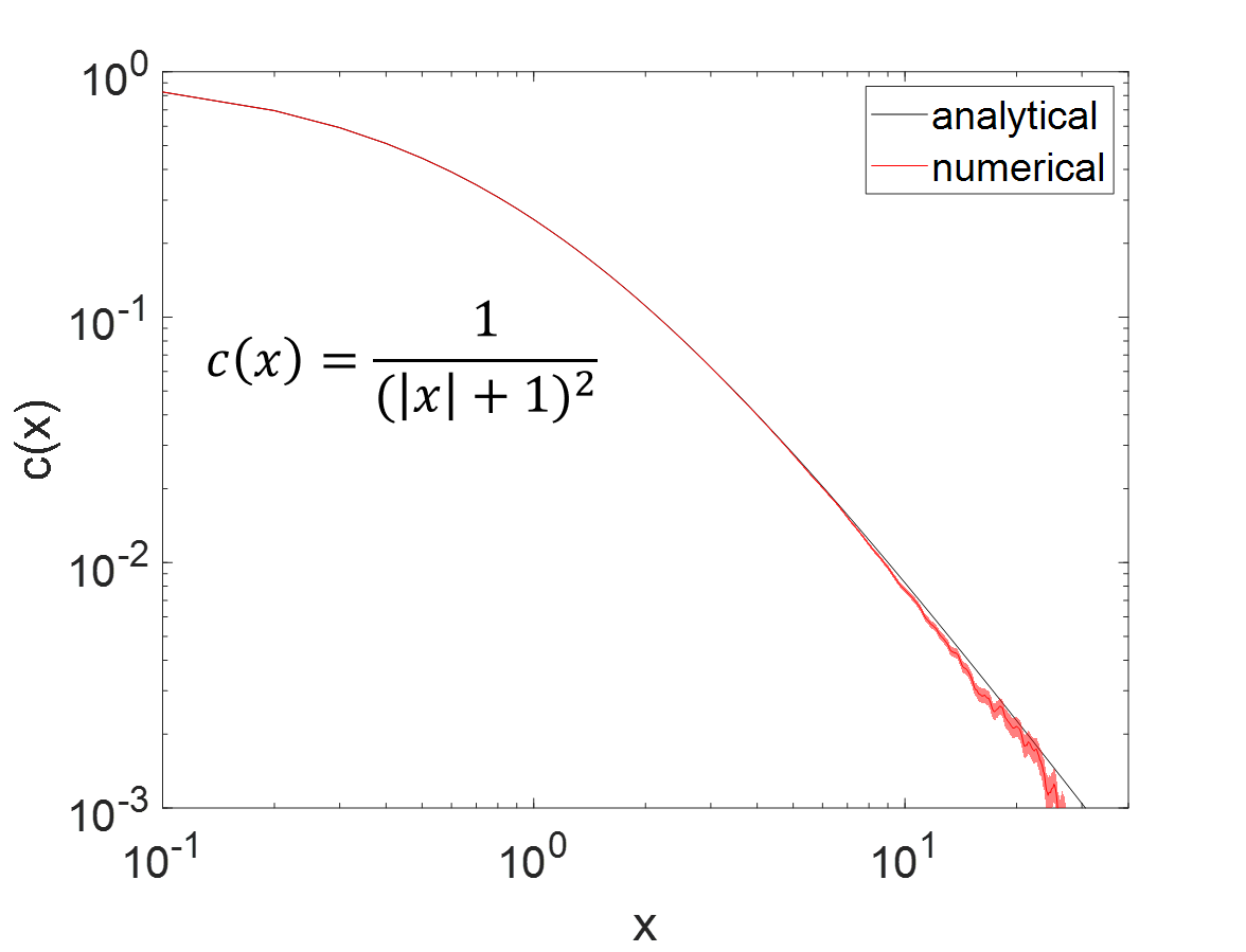
Figure 1: Autocorrelation $c(x)$ (in black) and the numerical evaluation of $\langle k(0)k(x)\rangle$ in red. The width of the red line is the numerical error of the mean for an averaging over 4000 configurations. The small systematic deviation at large $x$ is a finite size effect.

4 Localization for a quadratic decaying correlation function

We illustrate the effectiveness of equs. (16,19) with an example of a correlation function, which is long-ranged and which decays quadratically with distance:

$$c\left(x\right)=\frac{\sigma^{2}}{\left(\left|x/a\right|+1\right)^{2}},$$ (22)

with $a>0$ the correlation length and $\sigma^{2}=\langle k^{2}\rangle$ the disorder strength. The numerically computed correlation function obtained using equ. (20) is shown in fig. 1 and it matches the desired correlation function $c(x)$. The same procedure can be applied to any choice of correlation function. This is illustrated by comparing the disorder potential generated using equ. (22) (with $a=1$ and $\sigma=1$) and the Lorentzian correlation $(x^{2}+1)^{-1}$ using the same random sequence from equ. (20) but a different generating function $g$.

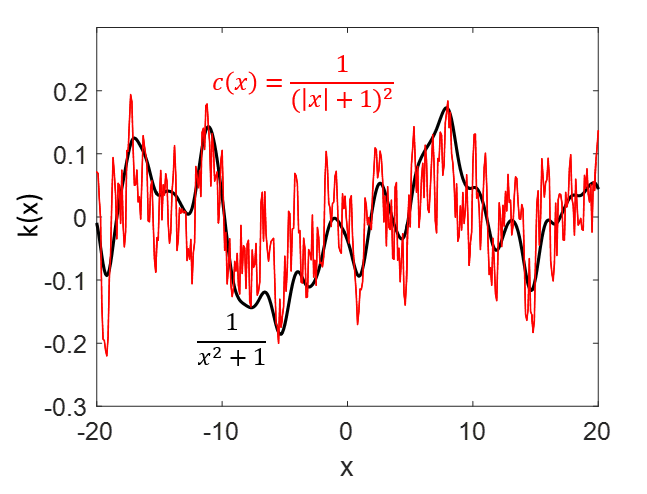
Figure 2: Ccorrelated potentials $k(x)$ for autocorrelations $c(x)=\frac{1}{(|x|+1)^{2}}$ (in red) and $\frac{1}{x^{2}+1}$ (in black).

We can compute explicitly the localization length associated to our choice of correlator $c(x)$ from equ. (22) using relations (15) and obtain for the various correlators (expressing only the case where $x$ is positive):

$$C(x) = \frac{\sigma^{2}x}{x/a+1}$$

$$\mathscr{C}(x) = \int_{0}^{x}dz\int_{0}^{z}dyc(y)=\sigma^{2}ax-\sigma^{2}a^{2}\ln\left[1+x/a\right]$$

$$C_{0}(x) = e^{-4\sigma^{2}ax}\left(1+x/a\right)^{4\sigma^{2}a^{2}}$$

$$C_{1}(x) = -2i\sigma^{2}xe^{-4\sigma^{2}ax}\left(1+x/a\right)^{4\sigma^{2}a^{2}-1}$$

$$C_{2}(x) = \left[\sigma^{2}(x/a+1)^{2}-4\sigma^{4}x.^{2}\right]e^{-4\sigma^{2}ax}\left(1+x/a\right)^{4\sigma^{2}a^{2}-2}.$$

The figure of the correlators (LABEL:C0bis) are shown in fig. 3

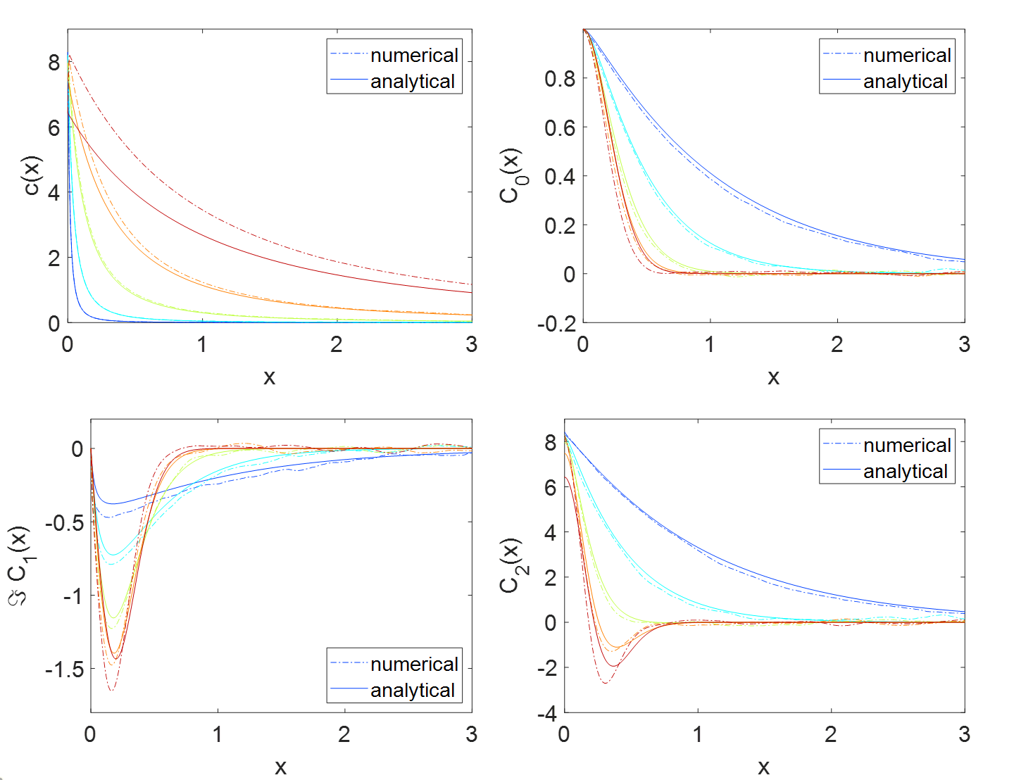
Figure 3: The correlators $C_{n}(x)$, where the dashed lines are numerical simulations (averaged over 10000 configurations), while the solid lines are the analytical expressions from equs. (LABEL:C0bis). The different colors correspond to different values of the correlation length ($a$) from blue to red (0.03, 0.08, 0.2, 0.6, 1.8).

An explicit expression for the Lyapounov exponent $\lambda$ can now be obtained by using (12) (see appendix A.4)

$$\lambda=\frac{y+\Im{I_{\lambda}}}{a(1-y)},$$ (24)

where

$$I_{\lambda}=\frac{[2aky+2ia^{2}(k^{2}-\sigma^{2})]e^{\bar{y}}\,\Gamma_{1+y}(\bar{y})}{\bar{y}^{y+1}},$$ (25)

$y=4a^{2}\sigma^{2}$ and $\bar{y}=y+2iak$.

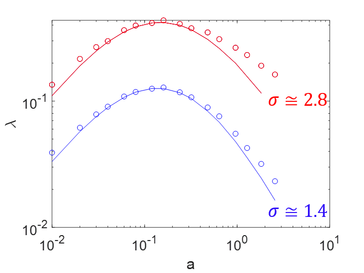
Figure 4: The Lyapounov exponent ($\lambda$) obtained numerically (symbols) and expression (24) (solid lines) as a function of the correlation length $a$ ($E=20$).

In fig. 4 we show the comparison between the numerically evaluated $\lambda$ and expression (24) for the case of strong disorder. The disorder correlation is given by $c(x)$ (equ. (22)). The overall agreement is very reasonable, in particular, when considering the wide range of correlation lengths $a$ and strong disorder.

5 Conclusion

In summary, we review a method to calculate the localization length for a disordered potential with an arbitrary autocorrelation function, which uses the addition of a small non-linear term in the wave equation. The Lyapounov exponent is calculated by evaluating several correlators explicitly. For a comparison between theory and numerical simulations, we introduced a method that can generate a disorder potential with an arbitrary disorder correlation. We compared favorably the numerical results of a particular long ranged disorder potential, whose autocorrelation decays quadratically with distance, with our theory and find an excellent agreement. This method is quite general can be used to study other types of correlated potentials and is not restricted to weak disorder.

Appendix A Appendix section

A.1 Evaluating $C_{0}(x)$

To evaluate the correlation functions $C_{n}(x)$ we consider $k(x)$ to be a random Gaussian variable with $\left\langle k(x)\right\rangle=0$. By definition, we have

$$C_{0}(x) = \left\langle e^{-2i\int_{0}^{x}k(x^{\prime})dx^{\prime}}\right\rangle$$

$$= \overset{\infty}{\underset{n=0}{\sum}}\frac{1}{n!}\left\langle\left[-2i\int_{0}^{x}k(x^{\prime})dx^{\prime}\right]^{n}\right\rangle$$

$$= \overset{\infty}{\underset{n=0}{\sum}}\frac{(-2i)^{n}}{n!}\int_{0}^{x}dx_{1}\cdots\int_{0}^{x}dx_{n}\left\langle k(x_{1})\cdots k(x_{n})\right\rangle.$$

For Gaussian random variables the odd number of correlators ($2n+1$) vanish

$$\left\langle k(x_{1})k\left(x_{2}\right)\cdots k(x_{2n+1})\right\rangle=0,$$ (27)

while for even number of correlators ($2n$) we have

$$\left\langle k(x_{1})k\left(x_{2}\right)\cdots k(x_{2n})\right\rangle = \left\langle k(x_{1})k\left(x_{2}\right)\rangle\cdots\langle k(x_{n-1})k(x_{2n})\right\rangle$$

$$+ \left\langle k(x_{1})k\left(x_{3}\right)\rangle\cdots\langle k(x_{n-1})k(x_{2n})\right\rangle$$

$$\cdots$$

$$+ \left\langle k(x_{1})k\left(x_{2n}\right)\rangle\cdots\langle k(x_{2n-2})k(x_{2n-1})\right\rangle.$$

Hence

$$C_{0}(x) = \overset{\infty}{\underset{n=0}{\sum}}\frac{(-2i)^{2n}}{(2n)!}\int_{0}^{x}dx_{1}\cdots\int_{0}^{x}dx_{n}\left\langle k(x_{1})\cdots k(x_{2n})\right\rangle$$ (29)

$$= \overset{\infty}{\underset{n=0}{\sum}}\frac{\left(-2i\right)^{2n}\left((2n-1)!!\right)}{(2n)!}\left[\int_{0}^{x}\int_{0}^{x}\left\langle k(x_{1})k(x_{2})\right\rangle dx_{1}dx_{2}\right]^{n}$$

$$= \overset{\infty}{\underset{n=0}{\sum}}\frac{1}{(n)!}\left[-2\int_{0}^{x}\int_{0}^{x}\left\langle k(x_{1})k(x_{2})\right\rangle dx_{1}dx_{2}\right]^{n}$$

$$= e^{-2\int_{0}^{x}\int_{0}^{x}\left\langle k(x_{1})k(x_{2})\right\rangle dx_{1}dx_{2}}.$$

This expression is similar to the result obtained in Li et al. (2016). The argument $arg$ of the exponential can be evaluated as

$$arg = -2\int_{0}^{x}\int_{0}^{x}\left\langle k(x_{1})k(x_{2})\right\rangle dx_{1}dx_{2}$$ (30)

$$= -2\int_{0}^{x}\int_{0}^{x}c(x_{1}-x_{2})dx_{1}dx_{2}$$

$$= -2\int_{-x}^{x}c(z)(x-|z|)dz$$

$$= -4\int_{0}^{x}c(z)(x-z)dz\quad\mbox{ assuming $c(-z)=c(z)$}$$

$$= -4\int_{0}^{x}dy\int_{0}^{y}dz\,c(z)$$

$$\equiv -4\int_{0}^{x}dy\,C(y)$$

$$\equiv -4\mathscr{C}(x).$$

Hence,

$$C_{0}(x)=e^{-4\mathscr{C}(x)}.$$ (31)

A.2 Evaluating $C_{1}(x)$

By definition, we have

$$C_{1}(x)=\left\langle k(0)e^{-2i\int_{0}^{x}k(x^{\prime})dx^{\prime}}\right\rangle.$$ (32)

Using the relations $\langle ab^{n}\rangle=n\langle ab\rangle\langle b^{n-1}\rangle$ for $a$ and $b$ two Gaussian variables, we have

$$C_{1}(x) = \left\langle k(0)e^{-2i\int_{0}^{x}k(x^{\prime})dx^{\prime}}\right\rangle$$ (33)

$$= \overset{\infty}{\underset{n=0}{\sum}}\frac{(-2i)^{n}}{(n)!}\left\langle k(0)\left(\int_{0}^{x}dx^{\prime}k(x^{\prime})\right)^{n}\right\rangle$$

$$= \left\langle k(0)\right\rangle+\overset{\infty}{\underset{n=0}{\sum}}\left\{\frac{2n+1}{(2n+1)!}\left\langle-2ik(0)\int_{0}^{x}k(x^{\prime})dx^{\prime}\right\rangle\right.$$

$$\times\left.\left(\frac{2n!}{2^{n}n!}\right)\left\langle\left(-2i\int_{0}^{x}k(x^{\prime})dx^{\prime}\right)^{2}\right\rangle^{n}\right\}$$

$$= -2i\int_{0}^{x}\langle k(0)k(x^{\prime})\rangle dx^{\prime}$$

$$\times\overset{\infty}{\underset{n=0}{\sum}}\frac{1}{n!}\left\langle-2\int_{0}^{x}\int_{0}^{x}k(x_{1})k(x_{2})dx_{1}dx_{2}\right\rangle^{n}$$

$$= -2i\int_{0}^{x}\langle k(0)k(x^{\prime})\rangle dx^{\prime}\times C_{0}(x)$$

$$= -2iC(x)C_{0}(x),$$

where we have defined

$$C(x)=\int_{0}^{x}\langle k(0)k(x^{\prime})\rangle dx^{\prime}.$$ (34)

A.3 Evaluating $C_{2}(x)$

Using the relations $\langle a^{2}b^{n}\rangle=\langle a^{2}\rangle\langle b^{n}\rangle+n\langle ab\rangle\langle ab^{n-1}\rangle$, $\langle a^{2}b^{n}\rangle=\left\langle a^{2}\right\rangle\left\langle b^{n}\right\rangle+n(n-1)\left\langle ab\right\rangle^{2}\left\langle b^{n-2}\right\rangle$ and $\left\langle b^{2n-1}\right\rangle=0$ for a and b Gaussian variables, we obtain

$$C_{2}(x) = \left\langle k^{2}(0)e^{-2i\int_{0}^{x}k(x^{\prime})dx^{\prime}}\right\rangle$$ (35)

$$= \overset{\infty}{\underset{n=0}{\sum}}\frac{(-2i)^{n}}{n!}\left\langle k^{2}(0)\left[\int_{0}^{x}dx^{\prime}k(x^{\prime})\right]^{n}\right\rangle$$

$$= \langle k^{2}(0)\rangle\overset{\infty}{\underset{n=0}{\sum}}\frac{(-2i)^{n}}{n!}\left\langle\left[\int_{0}^{x}dx^{\prime}k(x^{\prime})\right]^{n}\right\rangle$$

$$+ \overset{\infty}{\underset{n=2}{\sum}}\frac{(-2i)^{n}n(n-1)}{n!}\left\langle k(0)\int_{0}^{x}dx^{\prime}k(x^{\prime})\right\rangle^{2}$$

$$\times \left\langle\left[\int_{0}^{x}dx^{\prime}k(x^{\prime})\right]^{n-2}\right\rangle$$

$$= c(0)C_{0}(x)+\left\langle-2i\int_{0}^{x}k(0)k(x^{\prime})dx^{\prime}\right\rangle^{2}$$

$$\times \overset{\infty}{\underset{n=2}{\sum}}\frac{(-2i)^{n-2}}{(n-2)!}\left\langle\left[\int_{0}^{x}dx^{\prime}k(x^{\prime})\right]^{n-2}\right\rangle$$

$$= c(0)C_{0}(x)-4C^{2}(x)C_{0}(x).$$

A.4 Lyapounov exponent

The expression for $\lambda$ can be calculated as follows using equ. (12):

$$\lambda = -2\Re\left\{\int_{0}^{\infty}\left(k_{0}C_{1}(x)+C_{2}\left(x\right)\right)e^{-2ik_{0}x}dx\right\}$$

$$= -2ky\Im\left(\frac{e^{y+2iak}E_{-y}\left(y+2aik\right)}{y-1}\right)$$

$$-2a\Re\left(\frac{2\sigma^{2}+(k^{2}-\sigma^{2})e^{y+2iak}E_{-y}\left(y+2aik\right)}{y-1}\right)$$

$$= \frac{y+\Im\left\{e^{y+2iak}(y+2iak)^{-y-1}\Gamma_{1+y}(y+2iak)[2aky+2ia^{2}(k^{2}-\sigma^{2})]\right\}}{a(1-y)},$$

where the exponential integral is defined by

$$E_{\alpha}(z)=\int_{1}^{\infty}\frac{e^{-zt}}{t^{\alpha}}dt,$$ (37)

using $E_{\alpha}(z)=z^{\alpha-1}\Gamma_{1-\alpha}(z)$ and taking $y=4a^{2}\sigma^{2}$.

References

- Cutler and Mott (1969) M. Cutler and N. Mott, Physical Review 181, 1336 (1969).
- Thouless (1979) D. Thouless, Ill-Condensed Matter, edited by R. Balian, R. Maynard, and G. Toulouse (North-Holland, Amsterdam, 1979).
- Berthier and Biroli (2011) L. Berthier and G. Biroli, Reviews of Modern Physics 83, 587 (2011).
- Billy et al. (2008) J. Billy, V. Josse, Z. Zuo, A. Bernard, B. Hambrecht, P. Lugan, D. Clément, L. Sanchez-Palencia, P. Bouyer, and A. Aspect, Nature 453, 891 (2008).
- Roati et al. (2008) G. Roati, C. D’Errico, L. Fallani, M. Fattori, C. Fort, M. Zaccanti, G. Modugno, M. Modugno, and M. Inguscio, Nature 453, 895 (2008).
- Elson et al. (1983) J. Elson, J. Rahn, and J. Bennett, Applied Optics 22, 3207 (1983).
- John (1987) S. John, Physical review letters 58, 2486 (1987).
- Topolancik et al. (2007) J. Topolancik, B. Ilic, and F. Vollmer, Physical review letters 99, 253901 (2007).
- Hilke (2009) M. Hilke, Physical Review A 80, 063820 (2009).
- Karbasi et al. (2014) S. Karbasi, R. J. Frazier, K. W. Koch, T. Hawkins, and A. M. John Ballato, Nature Communications 5, 3362 (2014).
- Skipetrov (2014) S. E. Skipetrov, Nature nanotechnology 9, 335 (2014).
- Weaver (1990) R. Weaver, Wave motion 12, 129 (1990).
- Basko et al. (2006) D. Basko, I. Aleiner, and B. Altshuler, Annals of physics 321, 1126 (2006).
- Bardarson et al. (2012) J. H. Bardarson, F. Pollmann, and J. E. Moore, Physical review letters 109, 017202 (2012).
- Fishman et al. (1982) S. Fishman, D. Grempel, and R. Prange, Phys. Rev. Lett. 49, 509 (1982).
- Brandenberger and Craig (2012) R. Brandenberger and W. Craig, The European Physical Journal C 72, 1881 (2012).
- Hilke (2008) M. Hilke, Physical Review B 78, 012204 (2008).
- Huckestein (1995) B. Huckestein, Reviews of Modern Physics 67, 357 (1995).
- Anderson (1958) P. W. Anderson, Physical review 109, 1492 (1958).
- Abrahams et al. (1979) E. Abrahams, P. Anderson, D. Licciardello, and T. Ramakrishnan, Phys. Rev. Lett. 42, 673 (1979).
- Kunz and Souillard (1980) H. Kunz and B. Souillard, Communications in Mathematical Physics 78, 201 (1980).
- Pendry (1994) J. Pendry, Advances in Physics 43, 461 (1994).
- Cao (2003) H. Cao, Waves in random media 13, R1 (2003).
- Sanchez-Palencia et al. (2007) L. Sanchez-Palencia, D. Clément, P. Lugan, P. Bouyer, G. V. Shlyapnikov, and A. Aspect, Physical Review Letters 98, 210401 (2007).
- Hilke and Eleuch (2017) M. Hilke and H. Eleuch, Annalen der Physik 529, 1600347 (2017), 1600347.
- de Moura and Lyra (1998) F. A. de Moura and M. L. Lyra, Physical Review Letters 81, 3735 (1998).
- Izrailev and Krokhin (1999) F. Izrailev and A. Krokhin, Physical review letters 82, 4062 (1999).
- Shima et al. (2004) H. Shima, T. Nomura, and T. Nakayama, Physical Review B 70, 075116 (2004).
- Izrailev et al. (2012) F. M. Izrailev, A. A. Krokhin, and N. Makarov, Physics Reports 512, 125 (2012).
- Eleuch and Hilke (2015) H. Eleuch and M. Hilke, New Journal of Physics 17, 083061 (2015).
- Erdös and Herndon (1982) P. Erdös and R. Herndon, Advances in Physics 31, 65 (1982).
- Flores (1989) J. C. Flores, Journal of Physics: Condensed Matter 1, 8471 (1989).
- Dunlap et al. (1990) D. Dunlap, H.-L. Wu, and P. Phillips, Phys. Rev. Lett. 65, 88 (1990).
- Flores and Hilke (1993) J. Flores and M. Hilke, Journal of Physics A: Mathematical and General 26, L1255 (1993).
- Sánchez et al. (1994) A. Sánchez, E. Maciá, and F. Domínguez-Adame, Physical Review B 49, 147 (1994).
- Hilke and Flores (1997) M. Hilke and J. Flores, Physical Review B 55, 10625 (1997).
- Bellani et al. (1999) V. Bellani, E. Diez, R. Hey, L. Toni, L. Tarricone, G. Parravicini, F. Domínguez-Adame, and R. Gómez-Alcalá, Physical review letters 82, 2159 (1999).
- Hilke (1994) M. Hilke, Journal of Physics A: Mathematical and General 27, 4773 (1994).
- Hilke (2003) M. Hilke, Physical review letters 91, 226403 (2003).
- Tessieri (2002) L. Tessieri, Journal of Physics A: Mathematical and General 35, 9585 (2002).
- Eleuch et al. (2010) H. Eleuch, Y. Rostovtsev, and M. Scully, EPL (Europhysics Letters) 89, 50004 (2010).
- Eleuch and Rostovtsev (2010) H. Eleuch and Y. V. Rostovtsev, Journal of Modern Optics 57, 1877 (2010).
- Eleuch and Hilke (2018) H. Eleuch and M. Hilke, Results in Physics 11, 1044 (2018).
- Makse et al. (1995) H. Makse, S. Havlin, H. E. Stanley, and M. Schwartz, Chaos, Solitons & Fractals 6, 295 (1995).
- Usatenko et al. (2014) O. Usatenko, S. Melnik, S. Apostolov, N. Makarov, and A. Krokhin, Physical Review E 90, 053305 (2014).
- Li et al. (2016) F. Li, H. Zheng, and S.-Y. Zhu, Journal of Modern Optics 63, 1340 (2016).