Quantum Fisher Information with Coherence

Abstract

In recent proposals for achieving optical super-resolution, variants of the Quantum Fisher Information (QFI) quantify the attainable precision. We find that claims about a strong enhancement of the resolution resulting from coherence effects are questionable because they refer to very small subsets of the data without proper normalization. When the QFI is normalized, accounting for the strength of the signal, there is no advantage of coherent sources over incoherent ones. Our findings have a bearing on further studies of the achievable precision of optical instruments.

1 Introduction

Estimation and detection theory, formulated originally as a useful tool for signal analysis and efficient parameter estimation, became indispensable in quantum information processing, where the effects are subtle, signals are sparse, and any wasting of information is detrimental. However, these well-established techniques can be used even in classical detection schemes, with robust signals pushing the resolution to ultimate limits that have not been fully explored as yet.

Recent research pioneered by Tsang and collaborators, and inspired by a reconsideration of the classical Rayleigh criterion for the resolution of optical instruments such as telescopes or microscopes, has received considerable attention in the optical community (see [1] and references therein). The problem can be paraphrased: How well can we distinguish two bright spots? The celebrated Rayleigh arguments suggest that this can be done up to the distances when two blurred spots start to overlap. This rule of thumb can be justified by an analysis of the Fisher information for the intensity pattern, and one finds that the Fisher information vanishes for zero separation. As shown by Tsang and coworkers [2] and demonstrated experimentally [3], this behavior can be avoided if quantum estimation theory is adopted for the estimation of geometrical parameters, namely the transversal separation and the centroid positions of two equally bright spots with known intensities. In this context, the Fisher information refers to quantum measurements and becomes the Quantum Fisher Information (QFI) upon optimizing over all thinkable measurement schemes.

As shown in [4], however, the model used in [2] is not robust with respect to the inclusion of other parameters. When the intensities of the bright spots are considered as estimated parameters, together with the separation and the centroid, the QFI remains constant only if the two intensities are equal, but it drops to zero for unequal intensities. The unphysical situation of exactly equal intensities is singular and exhibits anomalous features.

The ongoing research on the estimation of optical effects addresses also the possible coherence of optical signals, and a recent discussion did not reach a consensus [5, 6, 7]. Whereas the paper [5] claims that the presence of coherence yields a QFI that vanishes for zero separation, the comment [6] shows by explicit calculations that this need not be so. The argument somehow paradoxically sticks to Rayleigh’s reasoning for incoherent image processing instead of applying the Sparrow resolution limit [8] and its modifications [9, 10, 11], which is the appropriate tool for quantifying the performance of (partially) coherent systems. According to the Sparrow criterion, two point sources can just be resolved when the second derivative of the image intensity vanishes at the point mid-way between the overlapping images of the two points. Particularly remarkable is the argumentation in favor of using an “anti-phase” superposition [10]: “Since the amplitude impulse response is an even function, zero intensity results at the mid-point between the two images whatever is the value of the separation. This suggests that, under ideal conditions, infinite resolution is approached.”

In this Letter, we explain the reasons for these misunderstandings on the basis of simple physical arguments and explicit calculations for an elementary model of a coherent superposition. Our central observation is quite simple: When coherence effects are taken into account, the Fisher information itself is no longer a meaningful measure of accuracy, because the channels exhibiting interference are not equivalent with respect to the strength of the signal. Indeed, the (Quantum) Fisher Information $F$ quantifies the content of information per registered particle; the Crámer–Rao inequality (here for a single parameter $\theta$),

$$(\Delta\theta)^{2}\geq H\equiv\frac{1}{{nF}}\,,$$ (1)

sets a bound on the precision $H$ with which $\theta$ can be estimated from the data. Here, $(\Delta\theta)^{2}$ is the expected value of the variance of the estimator, and $n$ is the number of detected particles. This number is just as important as the Fisher information in the product $nF$.

We recall that the Crámer–Rao bound on the precision in (1) is subject to two specific assumptions: (i) The estimator is unbiased; and (ii) the detection events are uncorrelated, they are independent and identically distributed (i.i.d.) random events. As a consequence of assumption (i) we have the unit numerator, while assumption (ii) is crucial for the product $nF$ in the denominator—the single-event Fisher information is multiplied by the number of detection events. One needs to verify that both assumptions are true in the situation of interest. Further, estimation is always model-dependent and, therefore, one must check the ingredients of the model that is used. We take for granted that all these verifications have been done.

2 Method and Results

Let us now elaborate on the argumentation for an ideal equal-weight superposition of symmetrically displaced sources. We phrase what follows in a quantum parlance, so a wave of complex amplitude $U(x)$ can be assigned to a ket $|U\rangle$, such that $U(x)=\langle x|U\rangle$, where $\langle{x}|$ is the bra for a point-like source at $x$. The quantum formulation (using these bra and ket symbols) facilitates the optimization since the intensity detection (and the corresponding complex amplitudes) need not represent an optimal scheme. More specifically, we denote by $\Psi(x)=\langle x|\Psi\rangle$ the amplitude of the (generic) point-spread function (PSF) of the coherent spatially-invariant imaging system. The coherence matrix relevant for the discussion is

$$\varrho=\frac{1}{N}|\Phi\rangle\langle\Phi|\quad\text{with}\quad|\Phi\rangle=|\Psi_{+}\rangle+e^{i\varphi}|\Psi_{-}\rangle\,.$$ (2)

Here, $|\Psi_{\pm}\rangle=\exp(\pm iPs/2)|\Psi\rangle$ are the spatially shifted PSF amplitudes, generated by the momentum operator $P$, $\langle x|P=-i\partial_{x}\langle x|$, and $N=\langle\Phi|\Phi\rangle=2[1+\mathop{\mathrm{Re}}\nolimits\bigl{(}e^{-i\varphi}\langle\Psi|e^{isP}|\Psi\rangle)]$ is the normalization. For notational simplicity, we do not indicate the dependence on the separation $s$ and the relative phase $\varphi$ in the superposition ket $|\Phi\rangle$, in $N$, or in $\rho$.

It is important to note that we are not dealing with a genuine quantum problem. We are using the quantum formalism for classical optics. The PSF amplitude $\Psi(x)$ is not a probability amplitude but a classical quantity, such as a component of the electric field. Therefore, $\Psi(x)$ is real, and the corresponding distribution for $P$ is even, so that $\langle f(P)\rangle=\langle\Psi|f(P)|\Psi\rangle=\langle f(-P)\rangle$ for all functions of $P$. In particular, then, $\langle P\rangle=0$ and there is no difference between $\langle P^{2}\rangle$ and the momentum variance of the PSF, ${(\Delta P)^{2}=\langle P^{2}\rangle-\langle P\rangle^{2}}$.

The QFI for the parameter $s$ can be calculated from the rank-1 expression $F=2\mathop{\mathrm{Tr}}\nolimits[(\partial_{s}\rho)^{2}]$, which yields

$$F_{\varphi}(s)=\frac{4}{N}\langle\partial_{{s}}\Phi|\partial_{{s}}\Phi\rangle-\frac{4}{N^{2}}\bigl{|}\langle\Phi|\partial_{{s}}\Phi\rangle\bigr{|}^{2}\,.$$ (3)

Note that it is as if the $s$-dependence of the normalization $N$ is ignored; in fact, its various contributions take care of each other. The analysis of the role of coherence in the parameter estimation hinges upon this expression for the QFI.

For understanding the role of coherence, the moment expansion for a small displacement $s\to 0$ is essential. A complication arises since $|\Phi\rangle=0$ when both $s=0$ and $\varphi=\pi$, so that $\rho$ is ill-defined in this limiting situation of destructive interference at vanishing separation, and it matters whether the limit $\varphi\to\pi$ succeeds or precedes the limit $s\to 0$. For $s=0$ and $\varphi\neq\pi$, one obtains

$$F_{\varphi}(0)=\tan^{2}(\varphi/2)(\Delta P)^{2}\,.$$ (4)

The QFI at $s=0$ is clearly diverging for $\varphi\to\pi$.

For $\varphi=\pi$, we have

$$F_{\pi}(s)=\frac{\langle P^{6}\rangle\langle P^{2}\rangle-\langle P^{4}\rangle^{2}}{36\langle P^{2}\rangle^{2}}s^{2}$$ (5)

for $s$ values so small that the terms proportional to $s^{4},s^{6},\dots$ can be ignored. Also for $\varphi=0$, the leading small-$s$ contribution is not given by (4); rather we have

$$F_{0}(s)=\frac{1}{4}\bigl{(}\Delta P^{2}\bigr{)}^{2}s^{2}\,,$$ (6)

which involves the variance of $P^{2}$. Figure 1 shows $F_{\varphi}(s)$ as a function of $s$ for several $\varphi$ values, for a Gaussian PSF.

It is amusing to note that the QFI for the coherent superposition with $\varphi=\pi/2$ equals exactly the limit of incoherent mixtures. This illustrates nicely Goodman’s observation [12] that “when (coherent) sources are in quadrature, the image intensity distribution is identical to that resulting from incoherent point sources.”

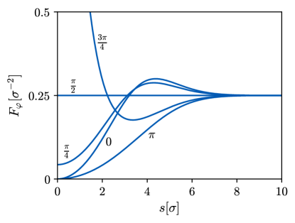
Figure 1: Dependence of the QFI on the displacement $s$ for the phase values $\varphi=0$, $\frac{1}{4}\pi$, $\frac{1}{2}\pi$, $\frac{3}{4}\pi$, and $\pi$. The QFI diverges for $\varphi\to\pi$. The plot is for a Gaussian PSF with the variances $(\Delta X)^{2}=\sigma^{2}$ and $(\Delta P)^{2}=1/(4\sigma^{2})$. The displacement is in units of $\sigma$, and $F$ in units of $\sigma^{-2}$.

3 Discussion

Understanding the behavior of the QFI for $\varphi=\pi$ is essential for the correct interpretation of the role of coherence in estimation problems. The QFI clearly exhibits a singularity when $s\to 0$ in this situation of destructive interference. Physically speaking, we are detecting a signal on a dark fringe, where the intensity is extremely low. If the norm $N=\langle\Phi|\Phi\rangle$ is taken as a weighting factor into the definition of the precision $H$ in (1), the singularity disappears. There are plausible and sound physical arguments for the inclusion of such a weight: constructive and destructive coherence is always manifested by an enhancement or a suppression of the emerging signal and this represents a valuable resource, which should be taken into account. This argument can be supported by an exact calculation of the cost of preparing the superposition in (2). The analysis can be linked to state-of the art technology [13] for the deterministic generation of these superpositions.

We generate the superposition in (2) from an entangled state,

$$|\varphi\rangle = 2^{-1/2}\bigl{(}|\Psi_{+}\rangle\otimes|\mathnormal{\uparrow}_{x}\rangle+e^{i\varphi}|\Psi_{-}\rangle\otimes|\mathnormal{\downarrow}_{x}\rangle\bigr{)}$$ (7)

$$= |\Phi_{1}\rangle\otimes|\mathnormal{\uparrow}_{z}\rangle+|\Phi_{2}\rangle\otimes|\mathnormal{\downarrow}_{z}\rangle\,,$$

where $|\Phi_{1}\rangle$ is half of the superposition in (2) and $|\Phi_{2}\rangle$ is that for $\varphi\to\varphi+\pi$,

$$|\Phi_{1}\rangle=\frac{1}{2}\bigl{(}|\Psi_{+}\rangle+e^{i\varphi}|\Psi_{-}\rangle\bigr{)}\,,\quad|\Phi_{2}\rangle=\frac{1}{2}\bigl{(}|\Psi_{+}\rangle-e^{i\varphi}|\Psi_{-}\rangle\bigr{)}\,,$$ (8)

and $|\mathnormal{\uparrow}_{x,z}\rangle$, $|\mathnormal{\downarrow}_{x,z}\rangle$ are the (pseudo-)spin states of an auxiliary qubit. The entanglement here is that available in classical light [14]. The desired coherent superpositions are obtained upon measuring the qubit in the $|\mathnormal{\uparrow}_{z}\rangle,|\mathnormal{\downarrow}_{z}\rangle$ basis, and the probabilities of occurrence are given by the norms of the respective superpositions, $\langle\Phi_{1}|\Phi_{1}\rangle$ and $\langle\Phi_{2}|\Phi_{2}\rangle$. If the probability that matters is very small, as is the case when dark-fringe data are selected, the procedure has a large overhead of discarded data, and a fair assessment cannot ignore these costs. Accordingly, there are three ways how to asses the QFI for such a generic scheme:

• From a joint measurement on the system and the qubit, for which the QFI is $F_{\text{ent}}=\langle P^{2}\rangle=(\Delta P)^{2}$, obtained by applying (3) to the entangled state $|\varphi\rangle$ in (7). While the optimal measurement may not be feasible, as it will require the distinction of entangled states, the value of $F_{\text{ent}}$ is an upper bound on the QFI from any other procedure.

• From the entangled state $|\varphi\rangle$, with the qubit traced out—only the system is measured. The resulting QFI is that for the incoherent mixture, $F^{\ }_{\text{inc}}=(\Delta P)^{2}$. Since $F^{\ }_{\text{inc}}=F_{\text{ent}}$, the entangled-basis measurements of scheme (E) offers no actual advantage.

• From measurements that are conditioned on finding the qubit in the state $|\mathnormal{\uparrow}_{z}\rangle$ or in the state $|\mathnormal{\downarrow}_{z}\rangle$. In this case, the data are sorted into two sub-ensembles, and their QFIs have to be weighted by their respective probabilities of occurrence to yield the total QFI,

  $$F^{\ }_{\text{tot}}(s) = \langle\Phi_{1}|\Phi_{1}\rangle F_{\varphi}(s)+\langle\Phi_{2}|\Phi_{2}\rangle F_{\varphi+\pi}(s)$$ (9)

  $$\leq \langle P^{2}\rangle=F^{\ }_{\text{ent}}=F^{\ }_{\text{inc}}\,.$$

  If the data of one sub-ensemble are ignored, then the respective term is removed from the sum, while the remaining term continues to be weighted by its probability of occurrence. As an immediate consequence of (4), together with $\langle\Phi_{1}|\Phi_{1}\rangle\bigr{|}_{s\to 0}=\cos^{2}(\varphi/2)$ and $\langle\Phi_{2}|\Phi_{2}\rangle\bigr{|}_{s\to 0}=\sin^{2}(\varphi/2)$, we have $F^{\ }_{\text{tot}}(0)=(\Delta P)^{2}=F^{\ }_{\text{inc}}$ except for $\phi=0$ or $\pi$. Figure 2 shows $F^{\ }_{\text{tot}}(s)$ as a function of $s$ for several $\varphi$ values, for a Gaussian PSF.

In view of this argumentation, it is clear that the coherence, although the QFI may diverge for one sub-ensemble, does not provide any improvement over an incoherent source, if the cost of generating such a signal is properly taken into account. Nothing is gained by an increase of the factor $F$ in the product $nF$ in (1) if the value of $n$ decreases even more.

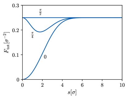
Figure 2: Dependence of the total QFI on the displacement $s$ for both constructive and destructive interference channels detected independently for phases $\varphi=0$, $\frac{1}{4}\pi$, and $\frac{1}{2}\pi$. This properly normalized QFI is always limited by its value for an incoherent superposition. Note that the upper bound is saturated for large displacements, and also for zero displacement for all the phases except when $\varphi=0$ or $\pi$. The plot is for a Gaussian PSF with the variances $(\Delta x)=\sigma^{2}$ and $(\Delta P)^{2}=1/(4\sigma^{2})$.

Other sorting schemes than scheme (S) can also be realized with the option of having situations intermediate between the fully coherent and the completely mixed sub-ensembles. In the case of partial coherence, the explicit form of the partially coherent state matters for the QFI of this sub-ensemble. The properly weighted total QFI for any sorting scheme, however, cannot exceed the upper bound set by $F_{\text{ent}}=F_{\text{inc}}$. This observation supports the arguments used in [5] and, so we think, settles the discussion in [5, 6, 7].

For simplicity, the discussion above deals with the estimation of a single parameter, the separation $s$, which is sufficient for demonstrating the case, namely that the sub-ensembles carry weights and these weights enter the total QFI in (9). When the data from an actual experiment are evaluated, however, the multi-parameter situation of asymmetrically displaced sources, with unequal intensity and partial coherence, matters. Then, the sub-ensembles are not specified by pure states like those in (8), but by rank-2 states of the generic form

$$\rho_{j}=\bigl{(}\begin{array}[]{cc}|\Psi_{+}\rangle&|\Psi_{-}\rangle\end{array}\bigr{)}R_{j}\Biggl{(}\begin{array}[]{c}\langle\Psi_{+}|\\ \langle\Psi_{-}|\end{array}\Biggr{)}\,,$$ (10)

where now $|\Psi_{\pm}\rangle=\exp\bigl{(}iP(s_{0}\pm s/2)\bigr{)}|\Psi\rangle$ and $R_{j}$ is a hermitian $2\times 2$ matrix restricted by $\rho_{j}\geq 0$ and $\mathrm{tr}(\rho_{j})=1$. In addition to the separation $s$ and the location parameter $s_{0}$, there are further parameters specifying the $R_{j}$s in accordance with the model considered. For each parameter, we have the QFI $F_{j}$ of the $j$th sub-ensemble, and the properly weighted sum of the $F_{j}$s replaces $F^{\ }_{\text{tot}}$ of (9). Together with the corresponding value of the count $n$, this yields the analog of the product $nF$ in the Crámer–Rao bound (1), provided that the usual conditions are met; in particular, the estimators must not be biased. The situations discussed in [5, 6, 7] are particular cases of this multi-parameter scenario.

Finally, concerning the so-called “Rayleigh curse” — a term coined in [2], where the value of the QFI at vanishing separation is by itself regarded as a significant measure for distinguishability, and $F(0)=0$ is the poor “classical” resolution (yes curse) while $F(0)>0$ is the superior “quantum” resolution (no curse) — we observe a few points. First, the estimator for the displacement $s$ usually exhibits a substantial bias when $s$ is small, and then the Crámer–Rao bound of (1) does not apply without the necessary modification. Second, the product $nF$ is relevant in (1), not just the Fisher information, and nothing is gained by an increase of $F$ if it is compensated for by a decrease of $n$; while an individual QFI in the sum in (9) can easily exceed $F_{\text{inc}}$, the properly weighted sum cannot.

4 Concluding remarks

The simple model studied here is sufficient to make the point that the QFI is but one ingredient and that there is no genuine advantage of coherent over incoherent sources when all aspects are accounted for. The model is good enough to explain the discrepancies in the analysis of coherent effects in [5, 6, 7]. But the model has its obvious limitations in that only one parameter is considered (the separation), and any analysis of a realistic situation has to deal with at least two more parameters, namely the centroid position and the relative intensity of the two sources. While there could be more parameters of relevance, such as the degree of coherence, certainly these three need to be estimated jointly from the data. A realistic analysis must also pay close attention on how the parameters are estimated from the data; the biases and the mean-square errors (or any other measure of accuracy) of the estimators actually used matter in practice, not the Crámer–Rao bound for optimal unbiased estimators. Clearly, much more work is needed before the community can reach a definite conclusion about the benefits of coherent sources, or coherent procedures for data acquisition, for the resolution of optical instruments.

5 Dedication

We dedicate this paper to the memory of Helmut Rauch (1939–2019), the pioneer of neutron interferometers, who taught us so much about the importance of coherence.

Funding Information

ZH and JŘ acknowledge financial support from the Grant Agency of the Czech Republic (Grant No. 18-04291S), LSS acknowledges financial support from the Spanish MINECO (Grant FIS2015-67963-P). The Centre for Quantum Technologies is a Research Centre of Excellence funded by the Ministry of Education and the National Research Foundation of Singapore.

References

- [1] M. Tsang, “Resolving starlight: a quantum perspective,” e-print arXiv:1906.02064[quant-ph] (2019).
- [2] M. Tsang, R. Nair, and X.-M. Lu, “Quantum theory of superresolution for two incoherent optical point sources,” \JournalTitlePhysical Review X 6, 031033 (2016).
- [3] M. Paúr, B. Stoklasa, Z. Hradil, L. L. Sánchez-Soto, and J. Řeháček, “Achieving the ultimate optical resolution,” \JournalTitleOptica 3, 1144–1147 (2016).
- [4] J. Řeháček, Z. Hradil, B. Stoklasa, M. Paúr, J. Grover, A. Krzic, and L. L. Sánchez-Soto, “Multiparameter quantum metrology of incoherent point sources: Towards realistic superresolution,” \JournalTitlePhysical Review A 96, 062107 (2017).
- [5] W. Larson and B. E. A. Saleh, “Resurgence of Rayleighs curse in the presence of partial coherence,” \JournalTitleOptica 5, 1382–1389 (2018).
- [6] M. Tsang and R. Nair, “Resurgence of Rayleigh’s curse in the presence of partial coherence: comment,” \JournalTitleOptica 6, 400–401 (2019).
- [7] W. Larson and B. E. A. Saleh, “Resurgence of Rayleigh’s curse in the presence of partial coherence: reply,” \JournalTitleOptica 6, 402–403 (2019).
- [8] C. M. Sparrow, “On spectroscopic resolving power,” \JournalTitleAstrophysical Journal 44, 76–86 (1916).
- [9] B. L. Mehta, “Two point resolution with non-uniform and non-symmetric illumination using partially coherent light,” \JournalTitleNouvelle Revue d’Optique 5, 95–99 (1974).
- [10] G. Cesini, G. Guattari, P. De Santis, and C. Palma, “Two-point resolution with anti-phase coherent illumination. I. One-dimensional systems,” \JournalTitleJournal of Optics 10, 79–87 (1979).
- [11] T. Asakura, “Resolution of two unequally bright points with partially coherent light,” \JournalTitleNouvelle Revue d’Optique 5, 169–177 (1974).
- [12] J. W. Goodman, Introduction to Fourier Optics (Roberts and Company Publishers, 3rd edition, 2005), p. 159.
- [13] B. Hacker, S. Welte, S. Daiss, A. Shaukat, S. Ritter, L. Li, and G. Rempe, “Deterministic creation of entangled atom-light Schrödinger cat states,” \JournalTitleNature Photonics 13, 110–115 (2019).
- [14] X.-F. Qian and J. H. Eberly, “Entanglement and classical polarization states,” \JournalTitleOptics Letters 36, 4110–4112 (2011).