Department of Physics, Kyoto Prefectural University of Medicine,
Kyoto 606-0823, Japan
yuho@koto.kpu-m.ac.jp
- and -duality rules among the gauge potentials in type II supergravities are studied. In particular, by following the approach of arXiv:1909.01335, we determine the - and -duality rules for certain mixed-symmetry potentials, which couple to supersymmetric branes with tension (). Although the -duality rules are rather intricate, we find a certain redefinition of potentials which considerably simplifies the duality rules. After the redefinition, potentials are identified with components of the -duality-covariant potentials, which have been predicted by the conjecture. We also discuss the field strengths of the mixed-symmetry potentials.
1 Introduction
Toroidally compactified 11D supergravity or type II supergravity has the -duality symmetry but this is not manifest in the standard formulation.
In order to exhibit the symmetry, the standard metric, scalar fields, and -form gauge potentials are not enough [1].
In fact, we additionally need to introduce certain mixed-symmetry potentials, which are related to the standard potentials through a non-local relation, similar to the electric-magnetic duality.
According to the conjecture [1, 2], there are infinitely many mixed-symmetry potentials in each theory.
By introducing an integer-valued parameter , known as the level, the number of mixed-symmetry potentials with a fixed level is finite, and we can determine the full list of the mixed-symmetry potentials for each level (see [3, 4] and references therein).
Although a list of mixed-symmetry potentials which constitutes the -duality multiplets has been algebraically determined, their physical definitions are still obscure.
In the case of the standard supergravity fields, their definitions can be fixed by the supergravity action, but the mixed-symmetry potentials do not appear in the standard supergravity action and it is not straightforward to specify their definitions.
A possible way to specify their definitions is to construct the worldvolume actions for supersymmetric branes.
As is well known, the Ramond–Ramond (R–R) fields couple to D-branes, and one can identify the definition of the R–R fields by looking at the Wess–Zumino (WZ) term.
Similarly, mixed-symmetry potentials generally couple to certain exotic branes [5, 6, 7, 8, 9, 10, 11, 12, 13, 14] and their definitions can be fixed by constructing the WZ term for exotic branes.
For example, the WZ term of the Kaluza–Klein (KK) monopole has been constructed in [15, 16, 17] and a precise definition of the dual graviton has been given.
However, at present, worldvolume actions have been constructed only for a few exotic branes.
To make precise definitions of mixed-symmetry potentials, it is more straightforward to determine the - and -duality transformation rule.
The mixed-symmetry potentials which couple to supersymmetric branes are related to the standard -form potentials under -/-duality transformations.
Then, by determining the duality rule, we can fix the convention for the mixed-symmetry potentials.
Recently, a systematic approach to determine the duality rules has been proposed in [18], and the -/-duality rules for the dual graviton have been determined.
In this paper, we continue the analysis and obtain the -/-duality rules for more mixed-symmetry potentials.
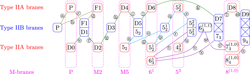
Concretely, we consider the duality web described in Figure 1.
There, each line (with a circled alphabet appended) corresponds to a -duality that connects a type IIA brane and a type IIB brane.
For example, the -duality ⓠ connects the -brane in type IIA theory and the -brane in type IIB theory.
Since the -brane and the -brane minimally couple to the potentials and , respectively, -duality ⓠ corresponds to a -duality rule for , where is the -duality direction.
We determine the -duality rule for the 27 lines, ⓐ–ⓩ, including non-linear terms in the duality rules.
In Figure 1, by following the notation of [9], a -brane in type II theory with tension
(1.1)
is denoted as a -brane.
In particular, the NS5-brane is denoted as and the fundamental string (F1) and the D-brane may be denoted as and , respectively.
The -dualities ⓐ–ⓓ and ⓔ–ⓜ correspond to the standard -dualities for the NS–NS fields and the R–R fields.
The -dualities ⓝ–ⓟ have been obtained in [16, 19, 20, 21, 18] and ⓧ is obtained in [10].
To the author’s knowledge, other -dualities are new.111In [19, 20], -duality rules for some additional potentials, which are not studied here, have been studied.
In our approach, type IIB fields are defined as -duality tensors, and the -duality rules are simple.
The structure of this paper is as follows.
In section 2, we fix our convention for the (bosonic) supergravity fields.
The standard fields are defined through the action, and several higher -form potentials are introduced through the electric-magnetic duality.
Additional mixed-symmetry potentials are defined in section 2.4 by finding a consistent parameterization of the -duality-covariant 1-form field .
In section 3, we determine the - and -duality rules by following the approach of [21, 18].
In particular, in sections 3.2.1 and 3.3.1, by considering certain field redefinitions, we show that our mixed-symmetry potentials can be packaged into the -covariant potentials , , and .
In section 4, we discuss the gauge symmetries and field strengths in each theory.
Section 5 is devoted to conclusions and discussions.
In Appendix A, we explain our conventions.
Figure 1: Duality web studied in this paper.
Type IIB branes are paired into -duality multiplets, though only supersymmetric branes are shown explicitly.
The M-theory uplifts of type IIA branes are displayed at the bottom.
Several different names for branes are as follows:
M-theory: , ,
Type IIA: , , , , ,
Type IIB: , , , , .
2 Supergravity fields
In this section, we fix our conventions for the bosonic supergravity fields.
2.1 11D supergravity
In 11D supergravity, the bosonic fields are and , for which the Lagrangian is
(2.1)
where we have defined .
By introducing the dual field strength as
(2.2)
the equation of motion for is expressed as the Bianchi identity
(2.3)
This suggests us to introduce the 6-form potential as
(2.4)
Although the potential is not contained in the standard Lagrangian, it is necessary for manifesting the -duality symmetry.
For the manifest -duality symmetry, in general, we need to introduce additional gauge potentials, which are generally mixed-symmetry tensors.
Among these, we consider , , and in this paper.
The dual graviton and the potential respectively appear in the worldvolume action of the KK monopole [15] and the M9-brane [23, 24, 25, 26], and their definitions are rather established.
However, for the -brane (which couples to ), only the kinetic term has been constructed in [27] and the WZ term including the potential has not been known.
Thus the definition of is still unclear.
Here, instead of considering brane actions, we define the mixed-symmetry potentials by using the approach of [18].
Namely, we consider the -duality-covariant 1-form , which appears when the eleven-dimensional spacetime is compactified on an -torus.
It is uniquely defined (as the generalized graviphoton [18]), and by parameterizing in terms of the mixed-symmetry potentials, we can fix the convention for the mixed-symmetry potentials.
The concrete parameterizations are given in section 2.4.
After providing the parameterizations, we can straightforwardly obtain the - and -duality transformation rules as explained in [18].
For convenience, below we summarize the correspondence between each gauge potential and the supersymmetric brane, which electrically couples to the potential:
(2.7)
2.2 Type IIA supergravity
In order to obtain type IIA supergravity, we consider the standard 11D–10D map,
(2.8)
where is the coordinate along the M-theory circle.
Then, we obtain the type IIA Lagrangian
(2.9)
where we have defined
(2.10)
and used the identity
(2.11)
Again, the equations of motion for and are expressed as Bianchi identities
(2.12)
where the dual field strengths are defined by
(2.13)
Then, we can introduce the dual potentials and as follows:
(2.14)
Through the electric-magnetic duality, we obtain the following 11D–10D map:
(2.15)
On the other hand, the equation of motion for is expressed as
(2.16)
and we can introduce the 7-form potential as
(2.17)
The 11D uplift of this 8-form field strength is discussed in section 4 [see Eq. (4.16)].
In 11D supergravity, we have introduced non-standard potentials , , and .
Here, we consider the following simple 11D–10D map for these potentials:222We do not consider overlined potentials, such as , which do not couple to supersymmetric branes.
(2.18)
The potential is related to the R–R 7-form introduced in (2.17) and the 9-form is related to the standard R–R 9-form (see section 3.1).
In the type IIA case, the correspondence between the potentials and the supersymmetric branes are summarized as follows:333We here ignore the component , which couples to the -brane.
(2.21)
2.3 Type IIB supergravity
The standard -duality-invariant (pseudo) Lagrangian for type IIB supergravity is
(2.22)
where are indices of doublets and .
The fundamental fields are , and is the Einstein-frame metric, for which the Hodge star operator is denoted by .
The scalar field is symmetric and satisfies
(2.23)
where we have raised or lowered the indices as and .
The field strengths are defined by
(2.24)
which satisfy the Bianchi identities
(2.25)
The self-duality relation for the 5-form field strength,
(2.26)
should be imposed at the level of equations of motion.
As is well-known, under the self-duality relation (2.26) the equation of motion for is equivalent to the last Bianchi identity.
If we additionally define the dual field strengths as444As noted in [10, 28], the triplet has only two independent components because it satisfies . Then, the duality (2.27) shows that the triplet also has only two independent components.
(2.27)
the equations of motion for and also can be expressed as the Bianchi identities
(2.28)
They suggest us to introduce the higher potentials, and as
(2.29)
(2.30)
In [28, 29, 30, 31], a 10-form potential was also introduced by considering the supersymmetry algebra (which is also predicted by [32]),555Additional 10-form potential was also introduced there, but here we do not consider this potential because this does not couple to supersymmetric branes. and the field strength, in our convention, is defined as
(2.31)
This satisfies the Bianchi identity (without considering the dimensionality)
(2.32)
In this paper, we consider the following set of type IIB fields:
(2.33)
which transform covariantly under -duality transformations.
At the present stage, definitions of , , , and are not specified.
They are defined in section 2.4.
In the following discussion, a redefinition of the 6-form potential
(2.34)
makes the -duality rules slightly shorter.
Thus, the 6-form rather than is mainly used in this paper.
For notational consistency, other fields also may be denoted by bold typeface,
The relation between the potentials and the supersymmetric branes are as follows:
(2.37)
It is noted that an -plet always couples to only two supersymmetric branes.
The components which couple to supersymmetric branes are and as discussed in [30, 33] (see also [4]).
2.4 Parameterization of the -duality-covariant 1-form
When 11D supergravity or type II supergravity is compactified to -dimensions, the bosonic fields with one external index are packaged into the 1-form field , where is the index for the so-called the vector representation of the -duality group () .
Under the compactification, we decompose the indices in M-theory/type IIB theory as
M-theory:
(2.38)
Type IIB theory:
(2.39)
Then the vector index in M-theory is decomposed into indices of tensors as [1]
(2.40)
where only the relevant components are shown.
In type IIB theory, the vector index is denoted by and it is decomposed into indices of tensors as [34]
(2.41)
Now, we parameterize each component of the 1-form field in terms of the bosonic fields introduced in the last subsections.
In fact, the 1-form has the universal form [18]
(2.42)
where / are the 11D/10D fields and / are the graviphoton, which are defined by
(2.43)
and similar for .
Therefore, the parameterization of the 1-form field is equivalent to the parameterization of the 11D- or 10D-covariant field or .
In this paper, we parameterize the 11D tensors as follows:
(2.44)
(2.45)
(2.46)
(2.47)
(2.48)
(2.49)
Here, the overlined indices are totally antisymmetrized; e.g. .
In addition, the equality
(2.50)
denotes that it is valid only for the indices satisfying the restriction rule,
(2.51)
Since the 1-form is uniquely defined, the above parameterizations uniquely define our bosonic fields, in particular, the mixed-symmetry potentials, , , and .
The detailed procedure, how to determine the above parameterization of is explained in section 2 of [18].
By considering the consistency between the M-theory and the type IIB parameterizations, the above parameterizations are uniquely determined (up to redefinitions of mixed-symmetry potentials).
The same parameterization can be obtained also by constructing a matrix representation of the generators as discussed in section 3 of [18].
In the second approach based on , the parameterizations will be completely determined without requiring the restriction rule (2.51) (see [18] for more details).
Now, let us turn to the type IIB parameterization.
In type IIB theory, we parameterize the -covariant 10D tensors as follows:
(2.52)
(2.53)
(2.54)
(2.55)
(2.56)
(2.57)
(2.58)
(2.59)
(2.60)
Here, the equality
(2.61)
denotes that it is valid only for the indices satisfying the restriction rules
(2.62)
Now, let us comment more on the restriction rules given in (2.51) and (2.62).
As already mentioned, our parameterizations of and are valid only for the restricted components.
One of the motivations of this paper is to provide a firm ground to study the worldvolume dynamics of exotic branes.
For that purpose, it will be enough to consider the restricted components, because the other components, which break the restriction rules, do not couple to any supersymmetric branes [30, 35, 36, 37, 33].
Components satisfying and breaking the rule are contained in different duality orbits, and they can be separated.
Indeed, in our parameterizations, the restricted components of and are always parameterized by the restricted components of mixed-symmetry potentials.
For example, in the parameterization of given in (2.48), as long as the rules is satisfied, the dual graviton appearing on the right-hand side also satisfies the rule .666This property can be spoiled by a redefinition; e.g. .
In this sense, our parameterizations respect the restriction rule, and the -duality rules obtained in the next section connect only the restricted components in type IIA/IIB theories.
In other words, components breaking the restriction rule do not appear in our -duality rules.
3 Duality rules
As it has been discussed in [18], the two 1-forms and are the same object expressed in different bases.
Indeed, they are related through a constant matrix as
(3.1)
which is called the linear map [21] (see also [38]).
In order to explain the linear map in more detail, let us further decompose the internal indices in M-theory and type IIB theory as
(3.2)
where and .
Under the decomposition, components of the 1-forms in M-theory and in type IIB theory are decomposed into tensors.
Then, the linear maps connect the tensors in the two theories.
In this paper, we consider the following linear maps (which are extensions of [21, 18]):
(3.3)
These relate the M-theory fields (left-hand side) and the type IIB fields (right-hand side), and by rewriting the M-theory fields in terms of type IIA fields, we obtain the -duality rules between type IIA/IIB theories.
By decomposing the indices into and , and taking into account of the restriction rule (2.51), we find that there are 27 linear maps.777For example, the restriction rule (2.51) for is and it gives two linear maps; and .
They correspond to the 27 -duality lines ⓐ–ⓩ depicted in Figure 1.
In the following subsections, we obtain the 27 -duality rules from the above linear maps.
Before proceeding, let us comment on the second restriction rule in type IIB theory (2.62).
Apparently, it looks different from the first restriction rule, but in fact both of them can be understood as a consequence of the M-theory rule (2.51) [4].
As an example, let us consider the last linear map .
The M-theory rule requires
(3.4)
and this leads to .
Then, the corresponding type IIB field need to satisfy and the second restriction rule in type IIB theory (2.62) is derived.
3.1 Standard potentials
Let us begin with a comparison of the linear maps ⓐ–ⓜ with the standard -duality rules.
For this purpose, we parameterize the type IIA fields and the -duality-covariant type IIB fields by using familiar fields.
We parameterize the 7-form and 9-form in type IIA theory as
(3.5)
and parameterize the type IIB fields as follows:
(3.6)
(3.7)
(3.8)
(3.9)
These parameterizations are given such that the linear maps ⓐ–ⓜ in (3.3) reproduce the standard -duality rules for NS–NS fields,
(3.10)
and R–R fields,
(3.11)
Here, the indices are 9D indices, which are orthogonal to the -duality direction or .
On the other hand, in the linear map (3.3), the indices are restricted to which run over the internal dimensions [recall (3.2)].
By assuming that the -duality rules have the 9D covariance, we have extended the linear map by replacing with .
This is always assumed in the following discussion.
Under the above parameterizations, the field strengths in type IIB supergravity become
(3.12)
where we have defined
(3.13)
(3.14)
(3.15)
By using the Hodge star operator in the string frame (), we obtain
(3.16)
(3.17)
The electric-magnetic duality for is considered further in section 3.4.
For later convenience, we also define the following 6-form, which has been used in [19]
(3.18)
We also introduce several redefinitions of the dual graviton.
The type IIB dual graviton 888In the literature (e.g. [16, 19]), the last index of the dual graviton is supposed to be a particular isometry direction, and it is not written down explicitly. Accordingly, the dual graviton is treated as a 7-form. introduced in [19] is related to our as
(3.19)
As we see below, this is useful to simplify the -duality rules (although the -duality covariance is not manifest).
In M-theory, we introduce
(3.20)
and define as .
More explicitly, we have
(3.21)
The type IIA dual graviton associated with a Killing direction (i.e. isometry direction) corresponds to of [19], and it is also useful to simplify the -duality rules.
3.2 Potentials for solitonic five branes
In this subsection, we consider the potentials that couple to the solitonic 5-branes (i.e. 5-branes with tensions ).
We begin by reproducing the known -duality rules ⓝ–ⓟ.
There, we demonstrate that redefinitions of potentials can make the -duality rules simpler.
After reproducing the known results, we obtain new -duality rules ⓠ–ⓢ.
In section 3.2.1, we find the field redefinitions, which make the -duality rules considerably simple, and discuss the relation to the potentials studied in the context of the double field theory (DFT) [39, 40, 41, 42, 43].
-duality rule ⓝ:
By substituting our parameterizations into the linear map , we find
(3.22)
(3.23)
They have been obtained in [16] (see Appendix A.2 for their conventions).
On the other hand, if we employ the -duality-covariant fields, we find
(3.26)
(3.27)
Since our linear maps (3.3) have the -duality covariance, the -duality rules are covariant under -duality.
In the present example, we can uplift the -duality rule (3.26) into
(3.28)
which indeed reproduce (3.26) by choosing .
On the other hand, gives
(3.29)
which corresponds to the -duality rule for R–R potentials obtained before.
Each of the -duality rules obtained in this paper has this kind of -dual partner.
They are partially obtained in Eq. (5.13) of [10] under the truncation .
The full result without the truncation is obtained in [18].
The same -duality map seems to be obtained in Eqs. (3.10) and (3.11) of [20], although the relation to our potentials is not clear.
On the other hand, by using the -duality covariant fields, we obtain
(3.42)
(3.43)
They are again self-dual under -duality.
A short comment
In the following, we present new results.
The -duality rules obtained below are rather lengthy, and we determine the maps only from type IIA fields to type IIB fields.
However, in section 3.2.1, we find a redefinition of mixed-symmetry potentials, which transforms our potentials into the potentials , , and .
The -duality rules for the new fields are very simple, and one can easily find the inverse map, if necessary.
-duality rule ⓠ:
The linear map gives
(3.44)
which is self-dual under -duality.
-duality rule ⓡ:
From the linear map , we obtain
(3.45)
Under the simplifying assumption , this map has been obtained in [10] [the last line of Eq. (5.12)], where corresponds to our (up to ).
The -dual counterpart of this -duality rule is obtained later in (3.69).
-duality rule ⓢ:
From the linear map , we obtain
(3.46)
The -dual counterpart of this -duality rule is found later in (3.70).
It may be possible to make the expression simpler by finding some -duality-covariant field redefinitions, but here do not attempt to find such redefinitions.
3.2.1 -dual-manifest redefinitions
Now, let us consider the field redefinition that makes the -duality rules very simple.
In the case of the R–R fields in type IIA/IIB theory, the R–R polyform in the -basis is defined as
(3.47)
By considering a redefinition into the -basis [44],
(3.48)
we find that the -duality rules for the new fields are simple [45]
(3.49)
This is according to the fact that the -basis transforms as an spinor.
As studied in [46, 47, 48], if we define the (real) gamma matrices that satisfy
(3.50)
and also define the Clifford vacuum as
(3.51)
where and (), we find that
(3.52)
transforms as an spinor.
Here, the R–R field is defined to have a definite chirality
(3.53)
Under the factorized -duality along the -direction, it transforms as
(3.54)
and in terms of the components, this transformation rule gives the rules (3.49).
Similarly, the potentials which couple to the solitonic 5-branes also constitute an -covariant potential denoted by [49], where the 20D indices are totally antisymmetric.
This tensor can be generally decomposed into tensors:
(3.55)
where the ellipsis denote the irrelevant contribution from the potentials that do not couple to supersymmetric branes.
Under the -duality along the -direction, this transforms as
(3.56)
where is a matrix, .
By rewriting the transformation rule in terms of the component fields , , , , and , we obtain
(3.57)
Similar to the case of the R–R potential , which is related to our potentials as (3.48), it is natural to expect that are also obtained by considering a redefinition of our mixed-symmetry potentials.
Indeed, if we redefine the type IIA fields as
(3.58)
(3.59)
(3.60)
and type IIB fields as
(3.61)
(3.62)
(3.63)
the complicated -duality rules obtained in this subsection are surprisingly simplified as (3.57).
As a consistency check, let us express the 7-form field strength in type IIA/IIB theory by using the new 6-form .
Then, we obtain
(3.64)
and they precisely coincide with the expression given in [49] up to conventions.
This shows that our are precisely the same as studied there, and they can be straightforwardly extended also to .
As shown in [50], the field strength, or , can be regarded as a particular component of999In terms of DFT, by supposing that is a generalized tensor with weight 1, we can show under generalized diffeomorphisms. The anomalous term vanishes under the assumptions that lower indices of , , and are associated with Killing directions.
(3.65)
where with .
The indices are raised/lowered by using and the derivative can be understood as .
Then, we can show that or in type IIA or IIB theory is reproduced from
(3.66)
Other components are also easily computed.
For example, the component associated with a Killing direction satisfying gives the field strength of the dual graviton,
(3.67)
In type IIA/IIB theory, this reproduces
(3.68)
where (note that ) .
The 11D uplift or the -duality-invariant expression is given respectively in section 4.1 or 4.2.
We can compute the other components as well, yielding the field strengths for mixed-symmetry potentials and .
Here, it will be useful to comment on the notion of the level .
If we look at, for example, the right-hand side of (3.63), terms like appear, but never appears.
This can be understood by considering the level, which has been introduced in the study of the conjecture [51, 52].
In type II theories, a potential which couples to a brane with the tension has the level [12].
For example, has level while the R–R potentials have level .
Since the potentials have level , the level on the right-hand side of (3.63) must be summed up to , and it is the reason why does not appear.
The level is always respected in various equations, such as the parameterization of given in section 2.4, the -duality rules, the field strengths such as (3.65), and the field redefinitions, and it helps when we find the complicated redefinitions such as (3.63).
3.3 Potentials for exotic branes
Here, we find the -duality rules for mixed-symmetry potentials that couple to exotic branes with tensions and .
Since the potentials have many indices, the -duality rules are generally more complicated than before.
Thus, we again find only the -duality rules, each of which maps a type IIA potential to type IIB potentials, and by using those, we identify the relation between our potentials and the manifestly -duality-covariant potentials.
-duality rule ⓣ: :
From the linear map , we obtain
(3.69)
This is -dual to the -dual rule (3.45).
Under , this map has been obtained in [10] [the middle line of Eq. (5.12)], where corresponds to (under ).
which is self-dual under -duality.
Under , this map has been obtained in [10] [the first line of Eq. (5.12)], where may be related to .
-duality rule ⓦ:
From the linear map , we obtain
(3.72)
-duality rule ⓧ:
From the linear map , we obtain
(3.73)
The inverse map has been obtained in Eq. (4.7) of [10],101010The correspondent of (3.73) has been given in Eq. (3.3) of [10], but there seems to be a small discrepancy regarding the terms including . and in our convention, we have
(3.74)
The -dual counterpart of this -duality is the map ⓛ connecting and .
-duality rule ⓨ:
From the linear map , we obtain
(3.75)
This is -dual to the -duality is the map ⓜ connecting and .
We can also find the inverse map as
(3.76)
So far, we have considered the potentials which couple to exotic -branes.
Finally, let us consider the only map, which is associated with branes with tension .
-duality rule ⓩ:
From the linear map , we find
(3.77)
The potentials and have level 4 while has level 3, and again we can see that the levels indeed match on both sides.
3.3.1 -dual-manifest redefinitions
Having obtained the -duality rules, let us find the field redefinitions that map our mixed-symmetry potentials to the -duality-covariant potentials.
As studied in [36], potentials ( and in type IIA/IIB theory) that couple to the exotic -branes constitute the -duality-covariant potential .
This transforms in the 87040-dimensional tensor-spinor representation of the group.
By using the notation of the spinor given in section 3.2.1, we denote it as that satisfies the following conditions:
(3.78)
As discussed in [50], if we truncate the components which do not couple to supersymmetric branes, can be parameterized as
(3.79)
(3.80)
(3.81)
The constraint is automatically satisfied under the restriction rule for the indices.
Under the factorized -duality along the -direction, it transforms as
(3.82)
and in terms of the components, we have
(3.83)
where and .
The -duality web for the family of potentials , which contains our -dualities ⓣ–ⓨ, can be summarized as follows:
(3.90)
Through trial and error, we have found that the following redefinitions indeed map our mixed-symmetry potentials to the -duality-covariant potentials :
Type IIA:
(3.91)
(3.92)
(3.93)
Type IIB:
(3.94)
(3.95)
(3.96)
Similarly, even for the potentials and , if we consider the redefinitions,
As is studied in [53, 54], potentials that couple to the -branes ( in type IIA/IIB theory) are packaged into the self-dual tensor .
Then, the above potentials, and , will be identified as the particular components of .
The potential contains the following family of potentials:
(3.104)
What we have explicitly confirmed is only the rightmost arrow ⓩ, but the existence of the -covariant potential suggests the validity of other maps.
Namely, we can define the family of potentials through the simple -duality rules,
(3.105)
for , without any non-linear correction.
Of course, in order to discuss the M-theory uplifts or the -duality rules for (), we need to determine how they enter into the 1-form field, or .
3.4 -duality rule
In this paper, the type IIB fields are defined to be -duality covariant, and under an transformation , the bosonic fields transform as
(3.106)
In particular, under the -duality, , the component fields are transformed as
(3.107)
It is sometimes useful to introduce the dual parameterization of ,
(3.108)
which is equivalent to
(3.109)
Then, the -duality rule becomes
(3.110)
The electric-magnetic duality for is also simplified as
(3.111)
For the -duality-covariant potentials, the -duality transformation rules are complicated.
For example, we find
(3.112)
(3.113)
(3.114)
The -duality rules for other -duality-covariant potentials also can be obtained from (3.107).
4 Field strengths and gauge transformations
In this section, we summarize the field strengths and gauge transformations studied in the literature in terms of our mixed-symmetry potentials, and make a small progress.
4.1 11D/Type IIA supergravity
In 11D supergravity, the field strengths and defined in section 2.1 are invariant under
(4.1)
Here, we discuss the field strengths for the mixed-symmetry potentials and .
Since and are 11D uplifts of the R–R 7-form and 9-form, let us consider the 11D uplifts of the known R–R field strengths and .
The 10-form is the electric-magnetic dual to the Romans mass [55], and in order to discuss the field strength of , we need to introduce the mass deformation.
Thus, let us begin by summarizing the gauge transformations and field strengths in massive type IIA supergravity.
In massive type IIA supergravity, the field strength in the -basis has the 0-form field strength ,
(4.2)
Accordingly, in the -basis, the field strength is given by
(4.3)
The gauge transformation is given by
(4.4)
Now, let us review the uplifts of these relations to 11D.
Since the R–R 1-form is contained in the 11D metric, under gauge transformations, the 11D metric is transformed as
(4.5)
where the coordinate is also transformed as .
The gauge transformations for the R–R 3-form and the -field are uplifted as
(4.6)
Under these transformations, the field strength,
(4.7)
transforms as
(4.8)
The non-invariance is due to , although and are invariant.
From a similar consideration, the gauge transformations for the R–R 5-, 7-, and 9-forms are also uplifted as111111In our convention, the gauge transformations of and does not include the mass deformation because the R–R potentials are included there such that the mass dependence is canceled out [see (3.5)]. The R–R 6-form potential is also contained in such that the mass dependence is canceled out, but the gauge transformation of the potential gives the mass dependence of .
(4.9)
(4.10)
(4.11)
and the associated field strengths are defined by
(4.12)
(4.13)
(4.14)
We note that the 7-form field strength is not invariant similar to the 4-form,
(4.15)
while the projections of the 9-form and the 11-form are invariant as it is clear from
(4.16)
The above gauge transformations have been discussed in [56, 15, 22, 25] and they are gauge symmetry of the “massive 11D supergravity” [56, 22, 25], which reproduce the massive type IIA supergravity after the dimensional reduction.
By using the above setup, we can easily consider the 11D uplift of the electric-magnetic duality .
For this purpose, we also introduce the 2-form field strength associated with a Killing vector as [25] (see also [20])
(4.17)
where .
This transforms as
(4.18)
In terms of the type IIA fields, we have , and this gives
(4.19)
Then, the electric-magnetic duality becomes
(4.20)
which shows that the dual graviton is electric-magnetic dual to the Killing vector.
In this paper, only the restricted component that couple to supersymmetric branes are considered, and the restriction corresponds to the projection in front of the field strength.121212The full definition of the field strength without the projection has been proposed in [20]. It can be found by regarding the dilaton equations of motion as the Bianchi identity, and by uplifting this to 11D.
We can similarly consider the 11D uplift of the electric-magnetic duality [25]
(4.21)
where
(4.22)
is the gauge-invariant field strength.
Now, we consider the relation to the recent studies on mixed-symmetry potentials in DFT.
If we decompose the 7-form field strength as
(4.23)
the 7-form field strength becomes
(4.24)
which coincides with the expression given in [50], and is invariant under
(4.25)
Here, we have parameterized
(4.26)
Let us also clarify the relation between the field strength of the dual graviton and the field strength defined in (3.68).
To this end, we assume the existence of a Killing direction denoted by (i.e. ) other than the M-theory circle.
For simplicity, we turn off the mass parameter.
Then, as before, we can easily show that the field strength
(4.27)
is invariant under
(4.28)
Now, we consider the reduction to type IIA theory.
We define the field strength of the dual graviton in type IIA theory as
(4.29)
which is also gauge invariant because is gauge invariant due to the Killing equation, .
Then, a straightforward but a bit long computation gives
(4.30)
where we have used (A.9).
This shows that the invariant field strength is the component of the untwisted tensor,
(4.31)
Indeed, we can easily check
(4.32)
Namely, the field strength is similar to the R–R field strength ; is invariant under gauge transformations of the R–R potentials, but not under -field gauge transformations, and it becomes invariant after untwisting the field strength as .
For completeness, let us also show that the gauge transformation (4.10) reproduces [15]
(4.33)
where we have parameterized
(4.34)
In terms of the -duality-covariant tensor, we have
(4.35)
The field strength also contains the field strength of the potential .
Since we have established the 11D–10D map, it is a straightforward task to compute the field strength.
The relation between and the potential is also given, and it will not be difficult to rewrite the field strength in a manifestly -duality-covariant form.
Similarly, we can also consider the reduction of the field strength , which gives the field strengths of and .
The former can be expressed in the -duality-covariant form by rewriting into .
Since this is a 9-form, we need to introduce another deformation parameter associated with the non-geometric -flux (with non-vanishing component ), which is the magnetic flux of the exotic -brane (see [57]).
On the other hand, the field strength of gives the field strength of the -duality-covariant potential , although the field strength automatically vanishes in 10D.
For the mixed-symmetry potential , it is not straightforward to define the field strength because it is not related to the standard fields.
However, since this is the 11D uplift of the type IIA potential , it may be useful to define the type IIA field strength by using the component and uplift this to 11D.
4.2 Type IIB supergravity
In type IIB supergravity, the gauge transformations are given as follows [28, 29, 30, 31]:
(4.36)
(4.37)
(4.38)
(4.39)
(4.40)
In terms of the component fields, we find
(4.41)
(4.42)
(4.43)
(4.44)
where the gauge parameters are parameterized as
(4.45)
and we have defined
(4.46)
Let us also consider the field strength for the dual graviton .
Similar to the case of type IIA supergravity, by introducing the untwisted tensor,
(4.47)
we define the field strength as
(4.48)
By assuming for an arbitrary field, it is invariant under the gauge transformation
(4.49)
which is the -dual counterpart of (4.35).
Since the dual graviton is -duality invariant, it is natural to expect that this field strength is invariant under -duality.
Indeed, we can express the field strength in a manifestly -duality-invariant form,
(4.50)
The gauge transformation (4.49) also can be expressed as
(4.51)
Here, we do not study additional potentials, but one can obtain their field strengths as follows.
As mentioned in the type IIA case, the field strength of will be obtained by computing .
Then, rewriting the field strength in terms of the -duality covariant potentials, we can obtain the field strength of .
In order to define the field strength of the potentials , it is useful to find the -duality-covariant expression for that reproduce the field strength as the particular component.
This covariant field strength contains various field strengths, and by using the relation between and our mixed-symmetry potentials, we can obtain the -duality-covariant expressions for field strengths.
5 Conclusions
In this paper, we have provided explicit definitions of mixed-symmetry potentials by finding their relation to the standard supergravity fields under - and -duality transformations.
The obtained -duality rules are generally very complicated, but by performing certain field redefinitions, they are considerably simplified.
The redefined fields , , , and are identified with certain components of the -covariant tensors , , , and .
These -covariant tensors have been studied in the literature, but their relation to the standard supergravity fields have not discussed enough.
For example, the potential has been expected to the -dual of the R–R 8-form , but the -duality rule (3.113), including the non-linear terms, is newly determined in this paper.
The -duality rule for and more mixed-symmetry potentials are also newly determined.
Additionally, we have also studied the field strengths of mixed-symmetry potentials.
Most of the results has been known in the literature (where the mixed-symmetry potentials are treated as -forms), but here we have clarified the relation to the field strength studied in DFT.
We have also provided the -duality-invariant expression for the field strength of the dual graviton.
The linear map has been originally studied for the generalized metric [38, 21, 18].
By comparing two parameterizations, duality rules for potentials that appear in the generalized metric () are determined.
The linear map for the 1-form studied here is more efficient to find the duality rules, but the parameterization is involved and the obtained -duality rules are rather long.
In the linear map for the generalized metric, the parameterization is more systematic, and by considering the linear map for the generalized metric, we may find a better definition of mixed-symmetry potentials which simplify the duality rules.
As we have demonstrated, the linear map works well in finding the duality rules for mixed-symmetry potentials, and it is a straightforward to consider more mixed-symmetry potentials.
In addition, having clarified the definitions of mixed-symmetry potentials, it is important to consider the application to the worldvolume theories of exotic branes.
It is also interesting to study the supersymmetry transformations for mixed-symmetry potentials (where Killing vectors should be involved) by extending the series of works [28, 29, 30, 31].
Before closing this paper, let us comment on a relevant open issue, called the exotic duality [58, 33, 49, 59, 60], which is the electric-magnetic duality for exotic branes with co-dimension equal to (or higher than) two.
As we have already mentioned, the mixed-symmetry potentials couple to various exotic branes electrically.
On the other hand, the exotic branes (with co-dimension two) magnetically couple to certain dual fields [61, 62, 63, 60, 64], such as the -fields131313This is originally introduced for example in [65, 66, 67, 68, 69] and utilized more recently in the -supergravity [70, 71, 72, 73, 74]. or the -fields [75, 74, 76, 60], which are associated with the non-geometric -flux [77] or the -fluxes [78, 79, 75].141414See [80, 81, 82, 83, 84, 85, 86, 87, 88, 89, 90, 91, 92, 93, 94, 95, 96, 97, 98, 99] for an incomplete list of references utilizing non-geometric fluxes.
Thus, the exotic duality is the electric-magnetic duality between the mixed-symmetry potentials and the dual potentials.
An example is given in (3.111),
(5.1)
where roughly corresponds to the -field (as we explain below).
Recently, the -duality-covariant expression of the exotic duality has been investigated in [100, 101, 102] but it has not yet fully succeeded.
For the -duality-covariant exotic duality, it will be important to establish the -duality-covariant description of the dual potentials, and we make a small attempt below.
First of all, let us explain the definition of the dual fields, such as the - and -fields.
In the -duality formulations, the supergravity fields are embedded into the generalized metric , which is defined as (see [103] and references therein)
(5.2)
where the generalized vielbein is the matrix representation of an element in the vector representation.
The identity matrix is invariant under the maximal compact subgroup, and the generalized vielbein is generally parameterized by the Borel subalgebra.
For example, in the type IIB theory, the Borel subalgebra is generated by
(5.3)
and the generalized vielbein can be parameterized as [34]
where the standard vielbein corresponds to .
On the other hand, we can also consider the negative Borel subalgebra, spanned by [64]
(5.4)
and introduce the dual parameterization as151515Our dual fields have opposite sign compared to those introduced in [21].
The dual vielbein is similarly defined by and the dual metric is .
Then, by comparing the two parameterizations of the generalized metric,
(5.5)
we can obtain the dual fields as a local redefinitions of the standard fields [64].
For example, if we consider only the NS–NS fields, the relation (5.5) is simplified as
(5.6)
where is the standard string-frame metric and is the dual-string-frame metric.
They are precisely the relations studied in the -supergravity [70, 71, 72, 73, 74].
On the other hand, if we only keep the metric and , the relation (5.5) reduces to
(5.7)
and this shows that the -field is similar to the appearing in (3.111).
In general, without any truncations, these relations receive non-linear corrections.
Secondly, let us explain the -duality rules for the dual fields.
By following the discussion of [21], the -duality rules for the dual fields are determined in the same manner as the standard potentials.
To this end, we parameterize the dual fields in the same manner as (3.6)–(3.9), for example,
(5.8)
Then, we find that the gamma fields follow the same -duality rules as those of the R–R field , although the position of the indices are opposite:161616The 11D uplifts also have the same form as the standard potentials.
(5.9)
The dual fields in the NS–NS sector also transform as
(5.10)
Then, we find that
(5.11)
transform covariantly under -duality, which reduce to (5.6) when only the NS–NS fields are present.
Similarly, we can show that the -field also transform covariantly under -duality.
For this purpose, we define the dual field associated with (or ) as
(5.12)
where and are poly-vectors and is the wedge product for poly-vectors.
This transforms as
(5.13)
under the -duality along the -direction.
In other words,
(5.14)
transforms as an spinor,171717To be more precise, it is a spinor density. The spinor has weight and the weight can be removed by considering . On the other hand, has weight and is weightless. where we have defined a new vacuum annihilated by ,
(5.15)
Other dual fields, such as [60, 64], also can be embedded into -duality tensors.
Finally, let us consider the exotic duality, in particular (5.1).
The left-hand side is the field strength of the potential .
Since is a component of , the field strength will be also defined covariantly.
The field strength has been discussed in [50], although the explicit form has not yet been determined,
(5.16)
On the other hand, the right-hand side contains , which is roughly equal to the -flux , as we have seen in (5.7).
The -flux may be also defined -duality covariantly,
(5.17)
and the exotic duality will be a covariant relation connecting and .
The non-trivial point is that although the field strength is defined in the standard parameterization, the -flux is defined in the dual parameterization, and it is not easy to find the relation.
In order to find the covariant expression for the exotic duality, it may be useful to consider the supergravity action for the dual fields.
As it has been (partially) worked out in [64], by substituting the dual parameterization into the action of the -duality-covariant supergravity, known as the exceptional field theory [104, 105, 106, 107] (which is based on DFT and earlier works [1, 2, 108, 109, 110, 111, 103, 112]), we obtain the action for the dual fields,
(5.18)
Then, the equations of motion for the dual fields are precisely the exotic duality, as discussed in [60].
Thus, in order to find the -duality-covariant exotic duality, it will be useful to find the -duality-covariant action for the dual fields, by defining the dual fields as -duality-covariant tensors.
From the covariant action, we obtain the -duality-covariant equations of motion for the dual fields, and they will correspond to the exotic duality.
Acknowledgments
We would like to thank José J. Fernández-Melgarejo and Shozo Uehara for useful discussions.
This work is supported by JSPS Grant-in-Aids for Scientific Research (C) 18K13540 and (B) 18H01214.
Appendix A Notations
A.1 Differential forms and mixed-symmetry potentials
We employ the following convention for differential forms:
(A.1)
where
(A.2)
The symmetrization and antisymmetrization are normalized as
(A.3)
Indices separated by “” are not (anti-)symmetrized.
For example,
(A.4)
When two groups of indices are antisymmetrized, we have used overlines.
For example,
(A.5)
In this paper, we consider only the components of the mixed-symmetry potentials that satisfy the restriction rule (2.51) or (2.62).
For convenience, by using the equality , we have expressed various equations without making the restriction rule manifest.
However, we can always convert the equality into the exact equality by making the restriction rule manifest.
For example, let us consider the equation (3.59),
(A.6)
In this example, the restriction rule is , and this is automatically satisfied by choosing .
We then obtain
(A.7)
In general, this makes the expressions longer, and that is the reason why we are using .
In order to simplify expressions, it is also useful to use the notation of the differential form.
For example, several relations for the -duality-covariant potentials become
(A.8)
(A.9)
(A.10)
(A.11)
(A.12)
(A.13)
(A.14)
(A.15)
A.2 Supergravity fields
Our gauge potentials are related to those used in [15, 17, 16, 10] as follows.
In type IIA theory, their fields (left) and our fields (right) are related as
(A.16)
where represents a Killing direction.
In type IIB theory, the relation is summarized as
(A.17)
Although the full -duality rule for the dual graviton has not been obtained there, by comparing the gauge transformation (4.51) with Eq. (B.4) of [16], we find
(A.18)
In addition, and correspond to our and at least under and .
We have not identified the precise relation between their and our .
Our 11D fields , , and are the same as those used in [15, 25, 26], where is denoted as .
The 9-form used in [25, 26] can be defined as
(A.19)
Let us also identify the relation between our type IIB fields and those used in [28, 29, 30, 31].
For this purpose, it is useful to perform a redefinition,
(A.20)
which makes the field strengths to have the schematic form ,
(A.21)
The gauge transformation also can be expressed as ,
(A.22)
by considering a field-dependent redefinitions of gauge parameters:
(A.23)
Then, the tilde potentials and the field strengths are related to the fields used in [28, 29, 30, 31] (appearing on the right-hand sides) as follows:
(A.24)
References
[1]
P. C. West,
“ and M theory,”
Class. Quant. Grav. 18, 4443 (2001)
[hep-th/0104081].
[2]
P. C. West,
“, SL(32) and central charges,”
Phys. Lett. B 575, 333 (2003)
[hep-th/0307098].
[3]
F. Riccioni and P. C. West,
“The origin of all maximal supergravities,”
JHEP 0707, 063 (2007)
[arXiv:0705.0752 [hep-th]].
[4]
J. J. Fernández-Melgarejo, Y. Sakatani and S. Uehara,
“Exotic branes and mixed-symmetry potentials I: predictions from symmetry,”
arXiv:1907.07177 [hep-th].
[5]
S. Elitzur, A. Giveon, D. Kutasov and E. Rabinovici,
“Algebraic aspects of matrix theory on ,”
Nucl. Phys. B 509, 122 (1998)
[hep-th/9707217].
[6]
M. Blau and M. O’Loughlin,
“Aspects of U duality in matrix theory,”
Nucl. Phys. B 525, 182 (1998)
[hep-th/9712047].
[7]
C. M. Hull,
“U duality and BPS spectrum of super Yang-Mills theory and M theory,”
JHEP 9807, 018 (1998)
[hep-th/9712075].
[8]
N. A. Obers, B. Pioline and E. Rabinovici,
“M theory and U duality on with gauge backgrounds,”
Nucl. Phys. B 525, 163 (1998)
[hep-th/9712084].
[9]
N. A. Obers and B. Pioline,
“U duality and M theory,”
Phys. Rept. 318, 113 (1999)
[hep-th/9809039].
[10]
E. Eyras and Y. Lozano,
“Exotic branes and nonperturbative seven-branes,”
Nucl. Phys. B 573, 735 (2000)
[hep-th/9908094].
[11]
E. Lozano-Tellechea and T. Ortin,
“7-branes and higher Kaluza-Klein branes,”
Nucl. Phys. B 607, 213 (2001)
[hep-th/0012051].
[12]
P. P. Cook and P. C. West,
“Charge multiplets and masses for ,”
JHEP 0811, 091 (2008)
[arXiv:0805.4451 [hep-th]].
[13]
J. de Boer and M. Shigemori,
“Exotic branes and non-geometric backgrounds,”
Phys. Rev. Lett. 104, 251603 (2010)
[arXiv:1004.2521 [hep-th]].
[14]
J. de Boer and M. Shigemori,
“Exotic Branes in String Theory,”
Phys. Rept. 532, 65 (2013)
[arXiv:1209.6056 [hep-th]].
[15]
E. Bergshoeff, E. Eyras and Y. Lozano,
“The Massive Kaluza-Klein monopole,”
Phys. Lett. B 430, 77 (1998)
[hep-th/9802199].
[16]
E. Eyras, B. Janssen and Y. Lozano,
“Five-branes, K K monopoles and T duality,”
Nucl. Phys. B 531, 275 (1998)
[hep-th/9806169].
[17]
E. Eyras and Y. Lozano,
“The Kaluza-Klein monopole in a massive IIA background,”
Nucl. Phys. B 546, 197 (1999)
[hep-th/9812188].
[18]
J. J. Fernández-Melgarejo, Y. Sakatani and S. Uehara,
“Exotic branes and mixed-symmetry potentials II: duality rules and exceptional -form gauge fields,”
arXiv:1909.01335 [hep-th].
[19]
A. K. Callister and D. J. Smith,
“Topological BPS charges in 10-dimensional and 11-dimensional supergravity,”
Phys. Rev. D 78, 065042 (2008)
[arXiv:0712.3235 [hep-th]].
[20]
A. K. Callister and D. J. Smith,
“Topological charges in SL(2,R) covariant massive 11-dimensional and Type IIB SUGRA,”
Phys. Rev. D 80, 125035 (2009)
[arXiv:0907.3614 [hep-th]].
[21]
Y. Sakatani and S. Uehara,
“Connecting M-theory and type IIB parameterizations in Exceptional Field Theory,”
PTEP 2017, no. 4, 043B05 (2017)
[arXiv:1701.07819 [hep-th]].
[22]
P. Meessen and T. Ortin,
“An Sl(2,Z) multiplet of nine-dimensional type II supergravity theories,”
Nucl. Phys. B 541, 195 (1999)
[hep-th/9806120].
[23]
E. Bergshoeff and J. P. van der Schaar,
“On M nine-branes,”
Class. Quant. Grav. 16, 23 (1999)
[hep-th/9806069].
[24]
E. Eyras and Y. Lozano,
“Brane actions and string dualities,”
Lect. Notes Phys. 525, 356 (1999)
[hep-th/9812225].
[25]
T. Sato,
“A Ten form gauge potential and an M9 brane Wess-Zumino action in massive 11-D theory,”
Phys. Lett. B 477, 457 (2000)
[hep-th/9912030].
[26]
T. Sato,
“On dimensional reductions of the M-nine-brane,”
hep-th/0003240.
[27]
T. Kimura, S. Sasaki and M. Yata,
“World-volume Effective Action of Exotic Five-brane in M-theory,”
JHEP 1602, 168 (2016)
[arXiv:1601.05589 [hep-th]].
[28]
E. A. Bergshoeff, M. de Roo, S. F. Kerstan and F. Riccioni,
“IIB supergravity revisited,”
JHEP 0508, 098 (2005)
[hep-th/0506013].
[29]
E. A. Bergshoeff, M. de Roo, S. F. Kerstan, T. Ortin and F. Riccioni,
“IIA ten-forms and the gauge algebras of maximal supergravity theories,”
JHEP 0607, 018 (2006)
[hep-th/0602280].
[30]
E. A. Bergshoeff, M. de Roo, S. F. Kerstan, T. Ortin and F. Riccioni,
“SL(2,R)-invariant IIB Brane Actions,”
JHEP 0702, 007 (2007)
[hep-th/0611036].
[31]
E. A. Bergshoeff, J. Hartong, P. S. Howe, T. Ortin and F. Riccioni,
“IIA/IIB Supergravity and Ten-forms,”
JHEP 1005, 061 (2010)
[arXiv:1004.1348 [hep-th]].
[32]
P. C. West,
“, ten forms and supergravity,”
JHEP 0603, 072 (2006)
[hep-th/0511153].
[33]
E. A. Bergshoeff and F. Riccioni,
“D-Brane Wess-Zumino Terms and U-Duality,”
JHEP 1011, 139 (2010)
[arXiv:1009.4657 [hep-th]].
[34]
I. Schnakenburg and P. C. West,
“Kac-Moody symmetries of 2B supergravity,”
Phys. Lett. B 517, 421 (2001)
[hep-th/0107181].
[35]
E. Bergshoeff, J. Hartong and D. Sorokin,
“Q7-branes and their coupling to IIB supergravity,”
JHEP 0712, 079 (2007)
[arXiv:0708.2287 [hep-th]].
[36]
E. A. Bergshoeff and F. Riccioni,
“Branes and wrapping rules,”
Phys. Lett. B 704, 367 (2011)
[arXiv:1108.5067 [hep-th]].
[38]
P. C. West,
“The IIA, IIB and eleven-dimensional theories and their common origin,”
Nucl. Phys. B 693, 76 (2004)
[hep-th/0402140].
[39]
W. Siegel,
“Two vierbein formalism for string inspired axionic gravity,”
Phys. Rev. D 47, 5453 (1993)
[hep-th/9302036].
[40]
W. Siegel,
“Superspace duality in low-energy superstrings,”
Phys. Rev. D 48, 2826 (1993)
[hep-th/9305073].
[41]
W. Siegel,
“Manifest duality in low-energy superstrings,”
hep-th/9308133.
[42]
C. Hull and B. Zwiebach,
“Double Field Theory,”
JHEP 0909, 099 (2009)
[arXiv:0904.4664 [hep-th]].
[43]
O. Hohm, C. Hull and B. Zwiebach,
“Generalized metric formulation of double field theory,”
JHEP 1008, 008 (2010)
[arXiv:1006.4823 [hep-th]].
[44]
E. Bergshoeff, R. Kallosh, T. Ortin, D. Roest and A. Van Proeyen,
“New formulations of D = 10 supersymmetry and D8 - O8 domain walls,”
Class. Quant. Grav. 18, 3359 (2001)
[hep-th/0103233].
[45]
S. F. Hassan,
“Supersymmetry and the systematics of T duality rotations in type II superstring theories,”
Nucl. Phys. Proc. Suppl. 102, 77 (2001)
[hep-th/0103149].
[46]
M. Fukuma, T. Oota and H. Tanaka,
“Comments on T dualities of Ramond-Ramond potentials on tori,”
Prog. Theor. Phys. 103, 425 (2000)
[hep-th/9907132].
[47]
O. Hohm, S. K. Kwak and B. Zwiebach,
“Unification of Type II Strings and T-duality,”
Phys. Rev. Lett. 107, 171603 (2011)
[arXiv:1106.5452 [hep-th]].
[48]
O. Hohm, S. K. Kwak and B. Zwiebach,
“Double Field Theory of Type II Strings,”
JHEP 1109, 013 (2011)
[arXiv:1107.0008 [hep-th]].
[49]
E. A. Bergshoeff and F. Riccioni,
“String Solitons and T-duality,”
JHEP 1105, 131 (2011)
[arXiv:1102.0934 [hep-th]].
[50]
E. Bergshoeff, A. Kleinschmidt, E. T. Musaev and F. Riccioni,
“The different faces of branes in Double Field Theory,”
JHEP 1909, 110 (2019)
[JHEP 2019, 110 (2020)]
[arXiv:1903.05601 [hep-th]].
[51]
T. Damour, M. Henneaux and H. Nicolai,
“E(10) and a ’small tension expansion’ of M theory,”
Phys. Rev. Lett. 89, 221601 (2002)
[hep-th/0207267].
[52]
P. C. West,
“Very extended E(8) and A(8) at low levels, gravity and supergravity,”
Class. Quant. Grav. 20, 2393 (2003)
[hep-th/0212291].
[53]
E. A. Bergshoeff, A. Marrani and F. Riccioni,
“Brane orbits,”
Nucl. Phys. B 861, 104 (2012)
[arXiv:1201.5819 [hep-th]].
[54]
E. A. Bergshoeff and F. Riccioni,
“Heterotic wrapping rules,”
JHEP 1301, 005 (2013)
[arXiv:1210.1422 [hep-th]].
[55]
L. J. Romans,
“Massive N=2a Supergravity in Ten-Dimensions,”
Phys. Lett. 169B, 374 (1986).
[56]
E. Bergshoeff, Y. Lozano and T. Ortin,
“Massive branes,”
Nucl. Phys. B 518, 363 (1998)
[hep-th/9712115].
[57]
J. J. Fernández-Melgarejo, T. Kimura and Y. Sakatani,
“Weaving the Exotic Web,”
JHEP 1809, 072 (2018)
[arXiv:1805.12117 [hep-th]].
[58]
E. A. Bergshoeff, T. Ortin and F. Riccioni,
“Defect Branes,”
Nucl. Phys. B 856, 210 (2012)
[arXiv:1109.4484 [hep-th]].
[59]
A. Chatzistavrakidis, F. F. Gautason, G. Moutsopoulos and M. Zagermann,
“Effective actions of nongeometric five-branes,”
Phys. Rev. D 89, no. 6, 066004 (2014)
[arXiv:1309.2653 [hep-th]].
[60]
Y. Sakatani,
“Exotic branes and non-geometric fluxes,”
JHEP 1503, 135 (2015)
[arXiv:1412.8769 [hep-th]].
[61]
F. Hassler and D. Lust,
“Non-commutative/non-associative IIA (IIB) Q- and R-branes and their intersections,”
JHEP 1307, 048 (2013)
[arXiv:1303.1413 [hep-th]].
[62]
D. Andriot and A. Betz,
“NS-branes, source corrected Bianchi identities, and more on backgrounds with non-geometric fluxes,”
JHEP 1407, 059 (2014)
[arXiv:1402.5972 [hep-th]].
[63]
T. Okada and Y. Sakatani,
“Defect branes as Alice strings,”
JHEP 1503, 131 (2015)
[arXiv:1411.1043 [hep-th]].
[64]
K. Lee, S. J. Rey and Y. Sakatani,
“Effective action for non-geometric fluxes duality covariant actions,”
JHEP 1707, 075 (2017)
[arXiv:1612.08738 [hep-th]].
[65]
A. D. Shapere and F. Wilczek,
“Selfdual Models with Theta Terms,”
Nucl. Phys. B 320, 669 (1989).
[66]
A. Giveon, E. Rabinovici and G. Veneziano,
“Duality in String Background Space,”
Nucl. Phys. B 322, 167 (1989).
[67]
M. J. Duff,
“Duality Rotations in String Theory,”
Nucl. Phys. B 335, 610 (1990).
[68]
A. A. Tseytlin,
“Duality Symmetric Formulation of String World Sheet Dynamics,”
Phys. Lett. B 242, 163 (1990).
[69]
A. Giveon, M. Porrati and E. Rabinovici,
“Target space duality in string theory,”
Phys. Rept. 244, 77 (1994)
[hep-th/9401139].
[70]
D. Andriot, M. Larfors, D. Lust and P. Patalong,
“A ten-dimensional action for non-geometric fluxes,”
JHEP 1109, 134 (2011)
[arXiv:1106.4015 [hep-th]].
[71]
D. Andriot, O. Hohm, M. Larfors, D. Lust and P. Patalong,
“A geometric action for non-geometric fluxes,”
Phys. Rev. Lett. 108, 261602 (2012)
[arXiv:1202.3060 [hep-th]].
[72]
D. Andriot, O. Hohm, M. Larfors, D. Lust and P. Patalong,
“Non-Geometric Fluxes in Supergravity and Double Field Theory,”
Fortsch. Phys. 60, 1150 (2012)
[arXiv:1204.1979 [hep-th]].
[73]
D. Andriot and A. Betz,
“-supergravity: a ten-dimensional theory with non-geometric fluxes, and its geometric framework,”
JHEP 1312, 083 (2013)
[arXiv:1306.4381 [hep-th]].
[74]
D. Andriot and A. Betz,
“Supersymmetry with non-geometric fluxes, or a -twist in Generalized Geometry and Dirac operator,”
JHEP 1504, 006 (2015)
[arXiv:1411.6640 [hep-th]].
[75]
G. Aldazabal, E. Andres, P. G. Camara and M. Grana,
“U-dual fluxes and Generalized Geometry,”
JHEP 1011, 083 (2010)
[arXiv:1007.5509 [hep-th]].
[76]
C. D. A. Blair and E. Malek,
“Geometry and fluxes of SL(5) exceptional field theory,”
JHEP 1503, 144 (2015)
[arXiv:1412.0635 [hep-th]].
[77]
J. Shelton, W. Taylor and B. Wecht,
“Nongeometric flux compactifications,”
JHEP 0510, 085 (2005)
[hep-th/0508133].
[78]
G. Aldazabal, P. G. Camara, A. Font and L. E. Ibanez,
“More dual fluxes and moduli fixing,”
JHEP 0605, 070 (2006)
[hep-th/0602089].
[79]
G. Aldazabal, P. G. Camara and J. A. Rosabal,
“Flux algebra, Bianchi identities and Freed-Witten anomalies in F-theory compactifications,”
Nucl. Phys. B 814, 21 (2009)
[arXiv:0811.2900 [hep-th]].
[80]
M. Ihl, D. Robbins and T. Wrase,
“Toroidal orientifolds in IIA with general NS-NS fluxes,”
JHEP 0708, 043 (2007)
[arXiv:0705.3410 [hep-th]].
[81]
D. Robbins and T. Wrase,
“D-terms from generalized NS-NS fluxes in type II,”
JHEP 0712, 058 (2007)
[arXiv:0709.2186 [hep-th]].
[82]
M. P. Hertzberg, S. Kachru, W. Taylor and M. Tegmark,
“Inflationary Constraints on Type IIA String Theory,”
JHEP 0712, 095 (2007)
[arXiv:0711.2512 [hep-th]].
[83]
U. H. Danielsson, S. S. Haque, G. Shiu and T. Van Riet,
“Towards Classical de Sitter Solutions in String Theory,”
JHEP 0909, 114 (2009)
[arXiv:0907.2041 [hep-th]].
[84]
B. de Carlos, A. Guarino and J. M. Moreno,
“Flux moduli stabilisation, Supergravity algebras and no-go theorems,”
JHEP 1001, 012 (2010)
[arXiv:0907.5580 [hep-th]].
[85]
B. de Carlos, A. Guarino and J. M. Moreno,
“Complete classification of Minkowski vacua in generalised flux models,”
JHEP 1002, 076 (2010)
[arXiv:0911.2876 [hep-th]].
[86]
U. Danielsson and G. Dibitetto,
“On the distribution of stable de Sitter vacua,”
JHEP 1303, 018 (2013)
[arXiv:1212.4984 [hep-th]].
[87]
J. Blåbäck, U. Danielsson and G. Dibitetto,
“Fully stable dS vacua from generalised fluxes,”
JHEP 1308, 054 (2013)
[arXiv:1301.7073 [hep-th]].
[88]
C. Damian, L. R. Diaz-Barron, O. Loaiza-Brito and M. Sabido,
“Slow-Roll Inflation in Non-geometric Flux Compactification,”
JHEP 1306, 109 (2013)
[arXiv:1302.0529 [hep-th]].
[89]
C. Damian and O. Loaiza-Brito,
“More stable de Sitter vacua from S-dual nongeometric fluxes,”
Phys. Rev. D 88, no. 4, 046008 (2013)
[arXiv:1304.0792 [hep-th]].
[90]
F. Hassler, D. Lust and S. Massai,
“On Inflation and de Sitter in Non‐Geometric String Backgrounds,”
Fortsch. Phys. 65, no. 10-11, 1700062 (2017)
[arXiv:1405.2325 [hep-th]].
[91]
P. Shukla,
“A symplectic rearrangement of the four dimensional non-geometric scalar potential,”
JHEP 1511, 162 (2015)
[arXiv:1508.01197 [hep-th]].
[92]
R. Blumenhagen, C. Damian, A. Font, D. Herschmann and R. Sun,
“The Flux-Scaling Scenario: De Sitter Uplift and Axion Inflation,”
Fortsch. Phys. 64, no. 6-7, 536 (2016)
[arXiv:1510.01522 [hep-th]].
[93]
P. Shukla,
“Reading off the nongeometric scalar potentials via the topological data of the compactifying Calabi-Yau manifolds,”
Phys. Rev. D 94, no. 8, 086003 (2016)
[arXiv:1603.01290 [hep-th]].
[94]
P. Shukla,
“Revisiting the two formulations of Bianchi identities and their implications on moduli stabilization,”
JHEP 1608, 146 (2016)
[arXiv:1603.08545 [hep-th]].
[95]
X. Gao, P. Shukla and R. Sun,
“Symplectic formulation of the type IIA nongeometric scalar potential,”
Phys. Rev. D 98, no. 4, 046009 (2018)
[arXiv:1712.07310 [hep-th]].
[96]
X. Gao, P. Shukla and R. Sun,
“On Missing Bianchi Identities in Cohomology Formulation,”
Eur. Phys. J. C 79, no. 9, 781 (2019)
[arXiv:1805.05748 [hep-th]].
[97]
P. Shukla,
“A dictionary for the type II non-geometric flux compactifications,”
arXiv:1909.07391 [hep-th].
[98]
P. Shukla,
“-dualizing the de-Sitter no-go scenarios,”
arXiv:1909.08630 [hep-th].
[99]
P. Shukla,
“Rigid non-geometric orientifolds and the swampland,”
arXiv:1909.10993 [hep-th].
[100]
E. A. Bergshoeff, V. A. Penas, F. Riccioni and S. Risoli,
“Non-geometric fluxes and mixed-symmetry potentials,”
JHEP 1511, 020 (2015)
[arXiv:1508.00780 [hep-th]].
[101]
E. A. Bergshoeff, O. Hohm, V. A. Penas and F. Riccioni,
“Dual Double Field Theory,”
JHEP 1606, 026 (2016)
[arXiv:1603.07380 [hep-th]].
[102]
E. A. Bergshoeff, O. Hohm and F. Riccioni,
“Exotic Dual of Type II Double Field Theory,”
Phys. Lett. B 767, 374 (2017)
[arXiv:1612.02691 [hep-th]].
[103]
D. S. Berman, H. Godazgar, M. J. Perry and P. West,
“Duality Invariant Actions and Generalised Geometry,”
JHEP 1202, 108 (2012)
[arXiv:1111.0459 [hep-th]].
[104]
O. Hohm and H. Samtleben,
“Exceptional Form of D=11 Supergravity,”
Phys. Rev. Lett. 111, 231601 (2013)
[arXiv:1308.1673 [hep-th]].
[105]
O. Hohm and H. Samtleben,
“Exceptional Field Theory I: covariant Form of M-Theory and Type IIB,”
Phys. Rev. D 89, no. 6, 066016 (2014)
[arXiv:1312.0614 [hep-th]].
[106]
O. Hohm and H. Samtleben,
“Exceptional field theory. II. E7(7),”
Phys. Rev. D 89, 066017 (2014)
[arXiv:1312.4542 [hep-th]].
[107]
O. Hohm and H. Samtleben,
“Exceptional field theory. III. E8(8),”
Phys. Rev. D 90, 066002 (2014)
[arXiv:1406.3348 [hep-th]].
[108]
F. Riccioni and P. C. West,
“-extended spacetime and gauged supergravities,”
JHEP 0802, 039 (2008)
[arXiv:0712.1795 [hep-th]].
[109]
C. Hillmann,
“Generalized coset dynamics and D=11 supergravity,”
JHEP 0903, 135 (2009)
[arXiv:0901.1581 [hep-th]].
[110]
D. S. Berman and M. J. Perry,
“Generalized Geometry and M theory,”
JHEP 1106, 074 (2011)
[arXiv:1008.1763 [hep-th]].
[111]
D. S. Berman, H. Godazgar, M. Godazgar and M. J. Perry,
“The Local symmetries of M-theory and their formulation in generalised geometry,”
JHEP 1201, 012 (2012)
[arXiv:1110.3930 [hep-th]].
[112]
D. S. Berman, M. Cederwall, A. Kleinschmidt and D. C. Thompson,
“The gauge structure of generalised diffeomorphisms,”
JHEP 1301, 064 (2013)
[arXiv:1208.5884 [hep-th]].