A double-pivot simplex algorithm and its upper bounds of the iteration numbers

Abstract

In this paper, a double-pivot simplex method is proposed. Two upper bounds of iteration numbers are derived. Applying one of the bounds to some special linear programming (LP) problems, such as LP with a totally unimodular matrix and Markov Decision Problem (MDP) with a fixed discount rate, indicates that the double-pivot simplex method solves these problems in a strongly polynomial time. Applying the other bound to a variant of Klee-Minty cube shows that this bound is actually attainable. Numerical test on three variants of Klee-Minty cubes is performed for the problems with sizes as big as $200$ constraints and $400$ variables. The test result shows that the proposed algorithm performs extremely good for all three variants. Dantzig’s simplex method cannot handle the Klee-Minty cube problems with $200$ constraints because it needs about $2^{200}\approx 10^{60}$ iterations. Numerical test is also performed for randomly generated problems for both the proposed and Dantzig’s simplex methods. This test shows that the proposed method is promising for large size problems.

Keywords: Double-pivot algorithm, simplex method, linear programming, Klee-Minty cube.

MSC classification: 90C05 90C49.

1 Introduction

Since Dantzig invented the simplex method in 1940s [3], its complexity has been a topic attracted many researchers. Since all pivot rules of the simplex method search the optimizer among vertices which are defined by the linear constraints, the iterate moves from one vertex to the next vertex along an edge of the polytope. Therefore, the diameter of a polytope, defined as the shortest path or the least number of edges between any two vertices of the polytope, is the smallest iteration number that the best simplex algorithm can possibly achieve. Hirsch in 1957 [4] conjectured that the diameter of the polytope is $m-n$ for the polytope $P=\{{\bf x}\in\mathbb{R}^{n}:{\bf A}{\bf x}\leq{\bf b}\}$ where ${\bf A}\in{\bf Z}^{m\times n}$ and $m>n$. This conjecture was disapproved by Santos [19] after a $50$-year effort of many experts. Now, some experts, for example Santos [20], believe that the diameter of the convex polytope can be bounded by a polynomial of $(m-n)n$. This conjectured upper bound for the diameter of the convex polytope is much smaller than the best-known quasi-polynomial upper bounds which are due to Kalai and Kleitman [11], Todd [24], and Sukegawa [22]. In a recent effort [26], this author showed that for a given polytope, the diameter is bounded by $\mathcal{O}\left(\frac{n^{3}\Delta}{\det({\bf A}^{*})}\right)$, where $\Delta$ is the largest absolute value among all $(n-1)\times(n-1)$ sub-determinants of ${\bf A}$ and ${\det({\bf A}^{*})}$ is the smallest absolute value among all nonzero $n\times n$ sub-determinants of ${\bf A}$.

Finding the diameter of convex polytopes provides only a surmised lowest iteration number for which an optimal pivot rule may achieve. Finding actually such a pivot rule (the way to choose the next neighbor vertex) is also a difficult problem. Researchers proposed many pivot rules with the hope that they may achieve an iteration number in the worst case bounded by a polynomial of $m$ and $n$ (see [23] and references therein). However, since Klee and Minty [16] constructed a cube and showed that Dantzig’s rule needs an exponential number of iterations in the worst case to solve the Klee and Minty cube problem, people have showed similar results for almost every popular pivot rule [1, 5, 7, 10, 17]. It is now believed that finding a pivot rule that will solve all linear programming problems in the worst case in a polynomial time is a very difficult problem [21].

Existing pivot rules consider one of many merit criteria to select an entering variable. Some popular pivot rules are, for example, the most negative index in the reduced cost vector (Dantzig’s rule), the best improvement rule, Bland’s least index pivoting rule, the steepest edge simplex rule, Zadeh’s rule, among others [23]. Each merit criterion has its own appealing feature. However, existing simplex algorithms cannot use multiple merits at the same time because each of these algorithms updates only one variable at a time. In a slightly different view, a merit criterion may be a good choice in most scenarios but may be a poor choice in some spacial case. For example, Dantzig’s rule is most efficient for general problems [18] but performs poorly for the Klee-Minty cube [16]. Therefore, randomized pivot rules [6, 12] that randomly select an entering variable from the set of possible entering variables that will improve the objective function have been proposed and proved to be able to find an optimizer in a polynomial time on average [12]. This shows that using a combination of merits in the selection of pivot can be beneficial.

In this paper, we consider a novel simplex algorithm for linear programming problem. This algorithm is different from all existing simplex algorithms in that it updates two variables at one iteration. This strategy looks two pivots ahead instead of focus only on the next step. We believe that this strategy is better than existing pivot rules because it looks longer term benefit instead of a short-sighted one-step achievement. Since the proposed algorithm updates two variables at a time, it considers multiple merits at the same time in the selection of the next vertex in a deterministic way which is different from the randomized rules. Numerical test shows that the proposed algorithm finds the optimal solution in just one iteration for three variants of Klee-Minty problems. We wish that these features give us some hope to find some strong polynomial algorithms to solve linear programming problems. We may extend the proposed algorithm to select more than two entering variables, but there is a trade-off between reducing iteration numbers and reducing the cost of each iteration.

After we finished this research, we realized that Vitor and Easton [25] recently proposed a similar idea to update two pivots at a time. Their algorithm chooses the two entering variables using the most negative reduced cost criterion rather than using a combined merit criteria to select the two entering variables. We indicate in Remark 2.1 that this is not a good strategy. Indeed, our numerical test shows that such a choice leads to an algorithm that needs exponentially many iterations to find the solution for Klee-Minty problems while our proposed algorithm needs just one iteration for these Klee-Minty problems.

In this paper, we use small letters with bold font for vectors and capital letters with bold font for matrices. To save space, we write the column vector ${\bf x}=[{\bf x}_{1}^{{\rm T}},{\bf x}_{2}^{{\rm T}}]^{{\rm T}}$ as ${\bf x}=({\bf x}_{1},{\bf x}_{2})$. The remainder of the paper is organized as follows. Section 2 describes the proposed algorithm. Section 3 provides two bounds of the iteration numbers of the algorithm. Section 4 presents the numerical test results for three variants of Klee-Minty cubes and compares the the performance of the proposed algorithm and Dantzig’s algorithm for randomly generated problems. The concluding remarks are in Section 5.

2 The proposed algorithm

We consider the primal linear programming problem in the standard form:

$$\begin{array}[]{cl}\min&{\bf c}^{{\rm T}}{\bf x},\\ \mbox{\rm subject to}&{\bf A}{\bf x}={\bf b},\hskip 7.22743pt{\bf x}\geq{\bf 0},\end{array}$$ (3)

where ${\bf A}\in{\mathbb{R}}^{m\times n}$, ${\bf b}\in{\mathbb{R}}^{m}$, ${\bf c}\in{\mathbb{R}}^{n}$ are given, and ${\bf x}\in{\mathbb{R}}^{n}$ is the vector to be optimized. Associated with the linear programming is the dual programming that is also presented in the standard form:

$$\begin{array}[]{cl}\max&{\bf b}^{{\rm T}}{\bf y},\\ \mbox{\rm subject to}&{\bf A}^{{\rm T}}{\bf y}+{\bf s}={\bf c},\hskip 7.22743pt{\bf s}\geq{\bf 0},\end{array}$$ (6)

where ${\bf y}\in{\mathbb{R}}^{m}$ is the dual variable vector, and ${\bf s}\in{\mathbb{R}}^{n}$ is the dual slack vector.

A feasible solution of the linear program satisfies the conditions of ${\bf A}{\bf x}={\bf b}$ and ${\bf x}\geq{\bf 0}$. We will denote by $B\subset\{1,2,\ldots,n\}$ the index set with cardinality $|B|=m$ and $N=\{1,2,\ldots,n\}\setminus B$ the complementary set of $B$ with cardinality $|N|=n-m$ such that matrix ${\bf A}$ and vector ${\bf x}$ can be partitioned as ${\bf A}=[{\bf A}_{B},{\bf A}_{N}]$ and ${\bf x}=({\bf x}_{B},{\bf x}_{N})$, moreover the columns of ${\bf A}_{B}$ are linearly independent and ${\bf A}_{B}{\bf x}_{B}={\bf b}$, hence ${\bf x}_{N}={\bf 0}$. We call this ${\bf x}=({\bf x}_{B},{\bf 0})$ as the basic feasible solution. Similarly, we can partition ${\bf c}$ and ${\bf s}$ according to the index sets $B$ and $N$ as follows:

$${\bf c}=\left[\begin{array}[]{c}{\bf c}_{B}\\ {\bf c}_{N}\end{array}\right],\hskip 14.45377pt{\bf s}=\left[\begin{array}[]{c}{\bf s}_{B}\\ {\bf s}_{N}\end{array}\right].$$

We denote by $\mathcal{B}$ the set of all bases $B$. In the discussion below, we make the following assumptions:

• $rank({\bf A})=m$.

• The primal problem (3) has an optimal solution.

• Initial basic feasible solution ${\bf x}^{0}$ is given and is not an optimizer.

• All basic feasible solutions are bounded above and below, more specifically, for all $i\in B\subset\mathcal{B}$, $\delta\leq x_{i}\leq\gamma$.

The first three assumptions are standard. The last assumption implies that the primal problem (3) is non-degenerate. Using the $B-N$ partition, we can rewrite the primal problem as

$$\begin{array}[]{cl}\min&{\bf c}_{B}^{{\rm T}}{\bf x}_{B}+{\bf c}_{N}^{{\rm T}}{\bf x}_{N},\\ \mbox{\rm subject to}&{\bf A}_{B}{\bf x}_{B}+{\bf A}_{N}{\bf x}_{N}={\bf b},\hskip 7.22743pt{\bf x}_{B}\geq{\bf 0},\hskip 7.22743pt{\bf x}_{N}\geq{\bf 0}.\end{array}$$ (9)

Since ${\bf A}_{B}$ is non-singular, we can rewrite (9) as

$$\begin{array}[]{cl}\min&{\bf c}_{B}^{{\rm T}}{\bf A}_{B}^{-1}{\bf b}+({\bf c}_{N}-{\bf A}_{N}^{{\rm T}}{\bf A}_{B}^{-{\rm T}}{\bf c}_{B})^{{\rm T}}{\bf x}_{N},\\ \mbox{\rm subject to}&{\bf x}_{B}={\bf A}_{B}^{-1}{\bf b}-{\bf A}_{B}^{-1}{\bf A}_{N}{\bf x}_{N},\hskip 7.22743pt{\bf x}_{B}\geq{\bf 0},\hskip 7.22743pt{\bf x}_{N}\geq{\bf 0}.\end{array}$$ (12)

Let superscript $k$ represent the $k$th iteration, the matrices and vectors in the $k$th iteration are then denoted by ${\bf A}_{B^{k}}$, ${\bf A}_{N^{k}}$, ${\bf c}_{B^{k}}$, ${\bf c}_{N^{k}}$, ${\bf x}_{B^{k}}$, ${\bf x}_{N^{k}}$, ${\bf s}_{B^{k}}$, and ${\bf s}_{N^{k}}$, where ${\bf x}^{k}=({\bf x}_{B^{k}},{\bf x}_{N^{k}})$ is the basic feasible solution of (3) with ${\bf x}_{B^{k}}>{\bf 0}$ and ${\bf x}_{N^{k}}={\bf 0}$. Similarly, we denote by ${\bf x}^{*}=({\bf x}_{B^{*}},{\bf x}_{N^{*}})$ the optimal basic solution of (3) with ${\bf x}_{B^{*}}={\bf A}_{B^{*}}^{-1}{\bf b}>{\bf 0}$ and ${\bf x}_{N^{*}}={\bf 0}$, by $({\bf y}^{*},{\bf s}^{*})$ the optimal basic solution of the dual problem (6) with ${\bf y}^{*}={\bf A}_{B^{*}}^{-{\rm T}}{\bf c}_{B^{*}}$, ${\bf s}_{B^{*}}={\bf 0}$, and ${\bf s}_{N^{*}}={\bf c}_{N^{*}}-{\bf A}_{N^{*}}^{{\rm T}}{\bf A}_{B^{*}}^{-{\rm T}}{\bf c}_{B^{*}}\geq{\bf 0}$, by $z^{*}={\bf c}^{{\rm T}}{\bf x}^{*}={\bf b}^{{\rm T}}{\bf y}^{*}$ the optimal value. It is worthwhile to note that the partition of $(B^{k},N^{k})$ keeps updating and it is different from the partition $(B^{*},N^{*})$ before an optimizer is found. Let

$$\bar{{\bf c}}_{N^{k}}^{{\rm T}}=({\bf c}_{N^{k}}-{\bf A}_{N^{k}}^{{\rm T}}{\bf A}_{B^{k}}^{-{\rm T}}{\bf c}_{B^{k}})^{{\rm T}}$$ (13)

be the reduced cost vector. Clearly, if $\bar{{\bf c}}_{N^{k}}\geq{\bf 0}$, an optimizer is found; if $\bar{c}_{j^{k}}<0$ for some $j^{k}\in N^{k}$, then an entering variable $x_{\jmath^{k}}$ in the next vertex is chosen from the set of $\{j^{k}~{}|~{}\bar{c}_{j^{k}}<0\}$ because by increasing $x_{\jmath^{k}}$, the objective function ${\bf c}^{{\rm T}}{\bf x}={\bf c}_{B^{k}}^{{\rm T}}{\bf x}_{B^{k}}+\bar{c}_{\jmath^{k}}x_{\jmath^{k}}$ will be reduced. Many different rules have been proposed for the selection of the entering variable $x_{\jmath^{k}}$ under the constraint:

$$\jmath^{k}\in\{j^{k}~{}|~{}\bar{c}_{j^{k}}<0\}.$$ (14)

Once the entering variable is selected, existing pivot rules determine the leaving variable using the following method: Denote $\bar{{\bf b}}={\bf A}_{B^{k}}^{-1}{\bf b}$ and $\bar{{\bf a}}_{\jmath^{k}}={\bf A}_{B^{k}}^{-1}{\bf A}_{\jmath^{k}}$, $\jmath^{k}\in N^{k}$ is the index of the entering variable, the leaving variable $x_{\imath}$, ${\imath}\in B^{k}$, is determined by the following condition.

$$x_{\imath}=\min_{i\in\{1,\ldots,m\}}\bar{b}_{i}/\bar{a}_{\jmath^{k},i},\hskip 7.22743pt\mbox{subject to}\hskip 7.22743pt\bar{a}_{\jmath^{k},i}>0.$$ (15)

The corresponding step-size is given by

$$\min_{i\in\{1,\ldots,m\}}\bar{b}_{i}/\bar{a}_{\jmath^{k},i},\hskip 7.22743pt\mbox{subject to}\hskip 7.22743pt\bar{a}_{\jmath^{k},i}>0.$$ (16)

As we pointed out above, our strategy is to select, in a deterministic way, two entering variables from the set of non-basic variables that will reduce the objective function. According to some extensive computational experience, for example [18], Dantzig’s rule is the most efficient on average among all popular pivot rules (even though Dantzig’s rule needs exponentially many pivots to find the optimal solution for Klee-Minty cubes in the worst case), therefore, we select the first entering variable $x_{\jmath_{1}^{k}}$ using Dantzig’s rule:

$${\jmath_{1}^{k}}:=\{{\jmath_{1}^{k}}~{}|~{}\bar{c}_{\jmath_{1}^{k}}=\min_{j^{k}\in N^{k}}\bar{{\bf c}}_{j^{k}}\}.$$ (17)

Kitahara and Mizuno [15] showed that the number of iterations in existing pivot rules is significantly affected by the minimum values of all the positive elements of primal basic feasible solutions. Carefully studying Klee-Minty cube and its variants [8, 13, 9] indicates that the other entering variable should be determined by taking the variable among all $j^{k}\in N^{k}$ with $\bar{c}_{j^{k}}<0$ such that a particular $\jmath_{2}^{k}$ will maximize the step-size defined in (16), i.e.,

$$x_{\jmath_{2}^{k}}=\max_{\bar{{\bf c}}_{j^{k}}<0}\Big{\{}\min_{i\in\{1,\ldots,m\}}\bar{b}_{i}/\bar{a}_{j^{k},i},\hskip 7.22743pt\mbox{subject to}\hskip 7.22743pt\bar{a}_{j^{k},i}>0\Big{\}}.$$ (18)

This strategy will be justified again in the proof of Theorem 3.2 and in the discussion of Remark 3.5. If ${\jmath_{2}^{k}}={\jmath_{1}^{k}}$ (which means that the most negative rule will generate the longest step), then we take the second entering variable $x_{\jmath_{2}^{k}}$ which has the second largest step-size.

Now we discuss how to choose the leaving variables. To make our notation simple, we drop the iteration index $k$ if it does not cause confusion. Let $\bar{{\bf A}}_{(\jmath_{1},\jmath_{2})}={\bf A}_{B}^{-1}{\bf A}_{(\jmath_{1},\jmath_{2})}$ where ${\bf A}_{(\jmath_{1},\jmath_{2})}$ is composed of the $\jmath_{1}$ and $\jmath_{2}$ columns of ${\bf A}_{N}$, and $\bar{{\bf c}}_{(\jmath_{1},\jmath_{2})}<{\bf 0}$ be the two corresponding elements in $\bar{{\bf c}}_{N}$. For the two entering indexes $(\jmath_{1},\jmath_{2})\in N^{k}$ such that that ${\bf x}_{(\jmath_{1},\jmath_{2})}=(x_{\jmath_{1}},x_{\jmath_{2}})\geq{\bf 0}$, we need

$${\bf x}_{B^{k}}^{k+1}={\bf A}_{B^{k}}^{-1}{\bf b}-{\bf A}_{B^{k}}^{-1}{\bf A}_{N^{k}}{\bf x}_{N^{k}}=\bar{{\bf b}}-\bar{{\bf A}}_{(\jmath_{1},\jmath_{2})}{\bf x}_{(\jmath_{1},\jmath_{2})}\geq{\bf 0}.$$ (19)

Therefore, the problem of finding a good new vertex is reduced to minimize the following linear programming problem.

$$\begin{array}[]{cl}\min&\bar{{\bf c}}_{(\jmath_{1},\jmath_{2})}^{{\rm T}}{\bf x}_{(\jmath_{1},\jmath_{2})},\\ \mbox{\rm subject to}&\bar{{\bf A}}_{(\jmath_{1},\jmath_{2})}{\bf x}_{(\jmath_{1},\jmath_{2})}\leq\bar{{\bf b}},\hskip 7.22743pt{\bf x}_{(\jmath_{1},\jmath_{2})}\geq{\bf 0}.\end{array}$$ (22)

Here the third merit criterion is introduced, which is to determine the values of the two entering variables to minimize the objective function under the constraints of (22).

Lemma 2.1

Let $z^{k}$ be the value of the objective function of (3) at iteration $k$. Then, the optimum of the problem (22) at iteration $k+1$ gives the minimal $z^{k+1}$ when the most negative and the longest step-size rules are used for two entering variables, and

$$z^{k+1}-z^{k}={\bf c}^{{\rm T}}{\bf x}^{k+1}-{\bf c}^{{\rm T}}{\bf x}^{k}.$$

• From (19), the constraints of (22) make sure that the updated ${\bf x}_{B^{k}}^{k+1}\geq{\bf 0}$ and the leaving variables are zeros. For variables in $N^{k}$, they will stay in zeros except two entering variables ${\bf x}_{(\jmath_{1},\jmath_{2})}\geq{\bf 0}$, and we may write variables in $N^{k}$ as a block vector ${\bf x}_{N^{k}}^{k+1}=({\bf x}_{(\jmath_{1},\jmath_{2})},{\bf 0})$. The improvement of ${\bf c}^{{\rm T}}{\bf x}^{k+1}-{\bf c}^{{\rm T}}{\bf x}^{k}$ is the optimal solution of (22), which is achieved when the optimal combination of the two entering variables is determined.       

As problem (22) has only two variables, the solution is slightly more complicate than the selection of a single entering variable in existing pivot rules, but is still simple and straightforward. We divide $\bar{{\bf A}}_{(\jmath_{1},\jmath_{2})}$ into two parts: $\bar{{\bf A}}_{1}$ has the rows with at least one positive element, and $\bar{{\bf A}}_{2}\leq{\bf 0}$ has the rows with all elements smaller than or equal to zero. Also we partition $\bar{{\bf b}}={\bf A}_{B}^{-1}{\bf b}$ into the corresponding $\bar{{\bf b}}_{1}$ and $\bar{{\bf b}}_{2}$. Since elements in $\bar{{\bf A}}_{2}$ are smaller than or equal to zero, in view of (19) or (22), introducing positive entering variables will keep the corresponding elements in ${\bf x}_{B^{k}}^{k+1}$ to be positive. For $\bar{{\bf A}}_{1}$, in view of (19) or (22), introducing positive variables may change the sign of some elements of ${\bf x}_{B^{k}}^{k+1}$. If the number of rows in $\bar{{\bf A}}_{1}$ is greater than or equal to $2$, for any two independent rows $(i_{1},i_{2})$ of $\bar{{\bf A}}_{1}$ denoted as $\bar{{\bf A}}_{1}(i_{1},i_{2})$, solving

$$\bar{{\bf A}}_{1}(i_{1},i_{2})\left[\begin{array}[]{c}x_{\jmath_{1}}\\ x_{\jmath_{2}}\end{array}\right]=\bar{{\bf b}}_{1}(i_{1},i_{2})$$ (23)

will give a possible vertex in the convex polygon defined in (22). Therefore ${\bf x}_{2}:=(x_{\jmath_{1}},x_{\jmath_{2}})\geq{\bf 0}$ is a feasible vertex of the polygon if $\bar{{\bf A}}_{1}{\bf x}_{2}\leq\bar{{\bf b}}_{1}$ holds. Otherwise, it is not feasible and will not be considered further. Two special feasible vertices, i.e., ${\bf x}_{2}:=(x_{\jmath_{1}},0)$ and ${\bf x}_{2}:=(0,x_{\jmath_{2}})$ which correspond to the most negative rule and the longest step-size rule respectively, should also be considered. For all feasible vertices of the convex polygon defined in (22), we select the vertex that minimizes the objective function of (22). The corresponding row indexes $(\imath_{1},\imath_{2})$ that form the selected vertex determine the leaving variables. If the number of rows in $\bar{{\bf A}}_{1}$ is exact one, the longest step pivot rule is used.

The proposed algorithm is therefore as follows:

Algorithm 2.1

Data: Matrix ${\bf A}$, vectors ${\bf b}$ and ${\bf c}$.  
Initial basic feasible solution ${\bf x}^{0}$, and its related partitions ${\bf x}_{B^{0}}$, ${\bf x}_{N^{0}}$, ${\bf A}_{B^{0}}$, ${\bf A}_{N^{0}}$, ${\bf c}_{B^{0}}$, ${\bf c}_{N^{0}}$, $({\bf A}_{B^{0}})^{-1}$, and $\bar{{\bf c}}_{N^{0}}^{{\rm T}}={\bf c}_{N^{0}}^{{\rm T}}-{\bf c}_{B^{0}}^{{\rm T}}({\bf A}_{B^{0}})^{-1}{\bf A}_{N^{0}}$.

• While $\min(\bar{{\bf c}}_{N^{k}})<0$

  • If at least two elements of $\bar{{\bf c}}_{N^{k}}$ are smaller than zero

    • The first entering variable $x_{\jmath_{1}^{k}}$ is determined by Dantzig’s rule. For all negative elements of $\bar{{\bf c}}_{N^{k}}$ other than the most negative elements $\bar{{\bf c}}_{\jmath_{1}^{k}}$, determine the $x_{\jmath_{2}^{k}}$ such that the second entering variable will take the longest step. Two special vertices, $(x_{\jmath_{1}^{k}},0)$ and $(0,x_{\jmath_{2}^{k}})$ are obtained.

    • Divide $\bar{{\bf A}}_{(}{\jmath_{1},\jmath_{2}})$ into two parts: $\bar{{\bf A}}_{1}$ whose row has positive elements and $\bar{{\bf A}}_{2}\leq{\bf 0}$. Partition ${\bf A}_{B^{k}}^{-1}{\bf b}$ into the corresponding $\bar{{\bf b}}_{1}$ and $\bar{{\bf b}}_{2}$.

    • If the number of rows of $\bar{{\bf A}}_{1}$ is greater than or equal to $2$

      • Compute all vertices in two dimensional plane by solving (23).

      • Determine all feasible vertices which satisfy ${\bf x}_{2}=(x_{\jmath_{1}},x_{\jmath_{2}})\geq{\bf 0}$ and $\bar{{\bf A}}_{1}{\bf x}_{2}\leq\bar{{\bf b}}_{1}$.

      • Find a pair of entering variables among all feasible vertices ${\bf x}_{2}$ (including the two special vertices) that minimizes the objective $[\bar{c}_{\jmath_{1}},\bar{c}_{\jmath_{2}}]{\bf x}_{2}$.

      • Update base ${\bf A}_{B^{k}}$ and ${\bf c}_{B^{k}}$, non-base ${\bf A}_{N^{k}}$ and ${\bf c}_{N^{k}}$. Compute ${\bf A}_{B^{k}}^{-1}$ and $\bar{{\bf c}}_{N^{k}}^{{\rm T}}={\bf c}_{N^{k}}^{{\rm T}}-{\bf c}_{B^{k}}^{{\rm T}}{\bf A}_{B^{k}}^{-1}{\bf A}_{N^{k}}$.

    • Else if there is only one row in $\bar{{\bf A}}_{1}$

      • The longest step rule is applied.

      • Update base ${\bf A}_{B^{k}}$ and ${\bf c}_{B^{k}}$, non-base ${\bf A}_{N^{k}}$ and ${\bf c}_{N^{k}}$. Compute ${\bf A}_{B^{k}}^{-1}$ and $\bar{{\bf c}}_{N^{k}}^{{\rm T}}={\bf c}_{N^{k}}^{{\rm T}}-{\bf c}_{B^{k}}^{{\rm T}}{\bf A}_{B^{k}}^{-1}{\bf A}_{N^{k}}$.

    • end (if)

  • Else if only one element of $(\bar{{\bf c}}_{N^{k}})$ is negative,

    • Dantzig’s rule (which is also the longest rule) is applied.

    • Update base ${\bf A}_{B^{k}}$ and ${\bf c}_{B^{k}}$, non-base ${\bf A}_{N^{k}}$ and ${\bf c}_{N^{k}}$. Compute ${\bf A}_{B^{k}}^{-1}$ and $\bar{{\bf c}}_{N^{k}}^{{\rm T}}={\bf c}_{N^{k}}^{{\rm T}}-{\bf c}_{B^{k}}^{{\rm T}}{\bf A}_{B^{k}}^{-1}{\bf A}_{N^{k}}$.

  • end (if)

  • $k\Leftarrow k+1$.

• end (while)

Remark 2.1

We can modify the algorithm by selecting two entering variables using the indexes corresponding to the two most negative elements in $\bar{{\bf c}}_{N^{k}}$ as [25]. In the numerical test section, we will see that this is a not a good strategy.

3 Bounds of the iteration numbers of the algorithm

In this section, we provide two upper bounds of the iteration numbers for the proposed algorithm using the strategy developed in [13, 15, 27].

Let $r$ be any real number and $\lceil r\rceil$ be the smallest integer bigger than $r$. Let $\gamma_{P}^{*}$ be the maximum value of all elements of ${\bf x}^{*}$ and

$$\gamma_{D}=\max_{k}\{\gamma_{D}^{k}\}=\max_{k}\Big{\{}\max_{j^{k}\in N^{k}}\{-\bar{c}_{j^{k}}~{}|~{}\bar{c}_{j^{k}}<0\}\Big{\}}.$$ (24)

Let $(B^{k},N^{k})$ be the partitions of base and non-base variables at iteration $k$ and $(B^{*},N^{*})$ be the partitions of base and non-base variables of the optimization solution. Let ${\bf x}^{*}$ be partitioned using $(B^{k},N^{k})$ but not $(B^{*},N^{*})$, i.e.,

$${\bf x}^{*}=\left[\begin{array}[]{c}{\bf x}_{B^{k}}^{*}\\ {\bf x}_{N^{k}}^{*}\end{array}\right].$$

The first lemma is derived using exactly the same argument but states a slightly improved result of [13, 15].

Lemma 3.1

(Kitahara and Mizuno) Let ${\bf x}^{*}$ be partitioned using $(B^{k},N^{k})$ and $z^{*}$ be the optimal value of (3), we have

$${\bf c}^{{\rm T}}{\bf x}^{k}-z^{*}\leq\gamma_{D}^{k}\|{\bf x}_{N^{k}}^{*}\|_{1}.$$ (25)

• Since ${\bf x}^{*}$ is partitioned using $(B^{k},N^{k})$, we have $({\bf x}_{B^{k}}^{*},{\bf x}_{N^{k}}^{*})\geq{\bf 0}$, and

  $${\bf A}_{B^{k}}{\bf x}_{B^{k}}^{*}+{\bf A}_{N^{k}}{\bf x}_{N^{k}}^{*}={\bf b}.$$

  This gives

  $${\bf x}_{B^{k}}^{*}={\bf A}_{B^{k}}^{-1}{\bf b}-{\bf A}_{B^{k}}^{-1}{\bf A}_{N^{k}}{\bf x}_{N^{k}}^{*}.$$

  Therefore, we have

  $${\bf c}^{{\rm T}}{\bf x}^{*} = {\bf c}_{B^{k}}^{{\rm T}}{\bf x}_{B^{k}}^{*}+{{\bf c}}_{N^{k}}^{{\rm T}}{\bf x}_{N^{k}}^{*}$$ (26)

  $$= {\bf c}_{B^{k}}^{{\rm T}}{\bf A}_{B^{k}}^{-1}{\bf b}-{{\bf c}}_{B^{k}}^{{\rm T}}{\bf A}_{B^{k}}^{-1}{\bf A}_{N^{k}}{\bf x}_{N^{k}}^{*}+{{\bf c}}_{N^{k}}^{{\rm T}}{\bf x}_{N^{k}}^{*}$$

  $$= {\bf c}_{B^{k}}^{{\rm T}}{\bf A}_{B^{k}}^{-1}{\bf b}+({{\bf c}}_{N^{k}}^{{\rm T}}-{{\bf c}}_{B^{k}}^{{\rm T}}{\bf A}_{B^{k}}^{-1}{\bf A}_{N^{k}}){\bf x}_{N^{k}}^{*}.$$

  Using this relation and (13), we have

  $$z^{*} = {\bf c}^{{\rm T}}{\bf x}^{*}$$ (27)

  $$= {\bf c}_{B^{k}}^{{\rm T}}{\bf A}_{B^{k}}^{-1}{\bf b}+\bar{{\bf c}}_{N^{k}}^{{\rm T}}{\bf x}_{N^{k}}^{*}$$

  $$\geq {\bf c}^{{\rm T}}{\bf x}^{k}-\gamma_{D}^{k}\|{\bf x}_{N^{k}}^{*}\|_{1}.$$

  This finishes the proof.       

Remark 3.1

If $B^{*}\neq B^{k}$, i.e., ${\bf x}^{k}$ is not an optimizer, from (27), it must have $\bar{{\bf c}}_{N^{k}}^{{\rm T}}{\bf x}_{N^{k}}^{*}<0$. Therefore, there is a $j^{k}\in N^{k}$ such that

$$\bar{c}_{j^{k}}<0\hskip 7.22743pt\mbox{and}\hskip 7.22743ptx_{j^{k}}^{*}>0.$$ (28)

This means that for $j^{k}\in N^{k}\cap B^{*}$, $x_{j^{k}}$ should be the entering variable. The problem is that one does not know $B^{*}$ before an optimizer is found.

We may also partition ${\bf x}^{k}$ using $(B^{*},N^{*})$ as

$${\bf x}^{k}=\left[\begin{array}[]{c}{\bf x}_{B^{*}}^{k}\\ {\bf x}_{N^{*}}^{k}\end{array}\right].$$

This gives

$${\bf A}_{B^{*}}{\bf x}_{B^{*}}^{k}+{\bf A}_{N^{*}}{\bf x}_{N^{*}}^{k}={\bf b},$$

and

$${\bf x}_{B^{*}}^{k}={\bf A}_{B^{*}}^{-1}{\bf b}-{\bf A}_{B^{*}}^{-1}{\bf A}_{N^{*}}{\bf x}_{N^{*}}^{k}.$$

Similar to the derivation of (25), we have

$${\bf c}^{{\rm T}}{\bf x}^{k}={\bf c}^{{\rm T}}{\bf x}^{*}+({{\bf c}}_{N^{*}}-{{\bf c}}_{B^{*}}{\bf A}_{B^{*}}^{-1}{\bf A}_{N^{*}})^{{\rm T}}{\bf x}_{N^{*}}^{k}=z^{*}+\bar{{\bf c}}_{N^{*}}^{{\rm T}}{\bf x}_{N^{*}}^{k}.$$

If $x_{j}^{k}>0$, we have $x_{j}^{k}\in B^{k}$. For $j\in{N^{*}}\cap B^{k}$, since $\bar{{\bf c}}_{N^{*}}\geq{\bf 0}$, we have

$$z^{*} \geq{\bf c}^{{\rm T}}{\bf x}^{k}-\max\{x_{j}^{k}~{}|~{}j\in N^{*}\cap B^{k}\}\|\bar{{\bf c}}_{N^{*}}\|_{1}.$$ (29)

Remark 3.2

If $N^{*}\neq N^{k}$, i.e., ${\bf x}^{k}$ is not an optimizer, it must have $\bar{{\bf c}}_{N^{*}}^{{\rm T}}{\bf x}_{N^{*}}^{k}>0$. Therefore, there is a $j^{*}\in N^{*}$ such that

$$\bar{c}_{j^{*}}>0\hskip 7.22743pt\mbox{and}\hskip 7.22743ptx_{j^{*}}^{k}>0.$$ (30)

This means that for $j^{*}\in N^{*}\cap B^{k}$, $0<x_{j^{*}}^{k}\in B^{k}$ should be the leaving variable. The problem is that one does not know $N^{*}$ before an optimizer is found.

Let $\gamma_{\ell}=\min_{k}x_{\jmath_{2}^{k}}$, where $x_{\jmath_{2}^{k}}$ is defined in (18), i.e., $x_{\jmath_{2}^{k}}$ is the longest step among all possible entering variables with $\bar{c}_{j^{k}}<0$ and $j^{k}\in N^{k}$; and define

$$\delta_{D}=\min_{k}\delta_{D}^{k}=\min_{k}\Big{\{}\min\{-\bar{c}_{j^{k}}~{}|~{}j^{k}\in N^{k}\hskip 7.22743pt\mbox{and}\hskip 7.22743pt\bar{c}_{j^{k}}<0\}\Big{\}}.$$ (31)

Considering Algorithm 2.1, our next lemma is an improvement of the one in [15].

Lemma 3.2

Let ${\bf x}^{k}$ and ${\bf x}^{k+1}$ be the $k$th and $(k+1)$th iterates generated by Algorithm 2.1. If ${\bf x}^{k}$ is not optimal and ${\bf x}^{k}\neq{\bf x}^{k+1}$, then, we have

$${\bf c}^{{\rm T}}{\bf x}^{k}-{\bf c}^{{\rm T}}{\bf x}^{k+1}\geq\delta_{D}\gamma_{\ell}.$$ (32)

• Since ${\bf x}^{k}\neq{\bf x}^{k+1}$, from Lemma 2.1, the difference of the objective functions between $k$th and $(k+1)$th iterations is actually the solution of (22), which is smaller than the special case when only one entering variable $x_{\jmath_{2}^{k}}$, which would generate the longest step among $\bar{c}_{j^{k}}<0$ for all $j^{k}\in N^{k}$, is selected. Let $\bar{{\bf x}}_{(\jmath_{1}^{k},\jmath_{2}^{k})}$ be the optimal solution of (22) at iteration $k$. Therefore

  $${\bf c}^{{\rm T}}{\bf x}^{k}-{\bf c}^{{\rm T}}{\bf x}^{k+1} = -\bar{{\bf c}}_{(\jmath_{1}^{k},\jmath_{2}^{k})}^{{\rm T}}\bar{{\bf x}}_{(\jmath_{1}^{k},\jmath_{2}^{k})}$$ (33)

  $$\geq -\bar{c}_{\jmath_{2}^{k}}~{}{x}_{\jmath_{2}^{k}}$$

  $$\geq \delta_{D}\gamma_{\ell}.$$

  This finishes the proof.       

Remark 3.3

Lemma 32 says that for Algorithm 2.1, the objective value decreases in every iteration by at least a constant $\delta_{D}\gamma_{\ell}$.

From Lemmas 25, 32 and Remark 3.3, it is easy to show that the following upper bound of iteration numbers of Algorithm 2.1 holds.

Theorem 3.1

Suppose that we generate a sequence of basic feasible solutions by Algorithm 2.1 from an initial iterate ${\bf x}^{0}$. Then, the number of total iterations is bounded above by

$$\Bigl{\lceil}\frac{{\bf c}^{{\rm T}}{\bf x}^{0}-z^{*}}{\delta_{D}\gamma_{\ell}}\Bigr{\rceil}\leq\Bigl{\lceil}\frac{\gamma_{D}^{0}\|{\bf x}^{*}\|_{1}}{\delta_{D}\gamma_{\ell}}\Bigr{\rceil}$$ (34)

• Since every iteration will reduce the objective function by at least a constant $\delta_{D}\gamma_{\ell}$, and the total difference between the initial objective function and the optimal objective function is ${\bf c}^{{\rm T}}{\bf x}^{0}-z^{*}$, we need at most

  $$\Bigl{\lceil}\frac{{\bf c}^{{\rm T}}{\bf x}^{0}-z^{*}}{\delta_{D}\gamma_{\ell}}\Bigr{\rceil}$$

  iterations to find the optimal solution. The bound of the left side of (34) is obtained. By the definition of $\gamma_{D}^{k}$, we have

  $$\bar{{\bf c}}_{N^{k}}^{{\rm T}}{\bf x}_{N^{k}}^{*}\geq-{\gamma_{D}^{k}\|{\bf x}_{N^{k}}^{*}\|_{1}}.$$

  Therefore, for initial step, the last inequality of (27) can be replaced by

  $${\bf c}^{{\rm T}}{\bf x}^{0}-z^{*}\leq\gamma_{D}^{0}\|{\bf x}^{*}\|_{1}.$$

  This shows the inequality of (34).       

Remark 3.4

The upper bound given in Theorem 34 is smaller than the one in [15] because (a) $\gamma_{\ell}$ is the smallest value in all longest steps among all iterates while the corresponding number in [15] is the smallest value in all nonzero components among all iterates ${\bf x}^{k}$, (b) $\|{\bf x}^{*}\|_{1}$ depends only on the optimal solution of ${\bf x}^{*}$, and (c) $\gamma_{D}^{0}$ depends only on the vector ${\bf c}$.

Now, we present an upper bound in terms of only $\delta$ and $\gamma$ defined in Assumption 4.

Theorem 3.2

Assume that the $k$th iterate generated by Algorithm 2.1 is not an optimizer. Let

$$t=m\frac{\gamma}{\delta}\log\left(m\frac{\gamma}{\delta}\right)$$ (35)

then there is a $\bar{j}\in B^{k}$, a corresponding $x_{\bar{j}}^{k}>0$, after at most another $\lceil t\rceil$ iterations, $x_{\bar{j}}^{k+t}$ becomes zero and stays there since then.

• In view of (27) in Lemma 25, since ${\bf x}^{*}$ has at most $m$ nonzero elements and $\bar{{\bf c}}_{N^{k}}^{{\rm T}}{\bf x}_{N^{k}}^{*}\geq-\gamma_{D}^{k}(m\gamma)$, we have

  $${{\bf c}}^{{\rm T}}{\bf x}^{k}-z^{*}\leq m\gamma\gamma_{D}^{k}.$$

  Using this inequality, together with Lemma 2.1, (33) in Lemma 32 and (17), we have

  $${\bf c}^{{\rm T}}{\bf x}^{k}-{\bf c}^{{\rm T}}{\bf x}^{k+1} = -\bar{{\bf c}}_{(\jmath_{1}^{k},\jmath_{2}^{k})}^{{\rm T}}\bar{{\bf x}}_{(\jmath_{1}^{k},\jmath_{2}^{k})}$$

  $$\geq -\bar{c}_{\jmath_{1}^{k}}~{}{x}_{\jmath_{1}^{k}}$$

  $$\geq \gamma_{D}^{k}\delta$$

  $$\geq \frac{\delta}{m\gamma}\left({{\bf c}}^{{\rm T}}{\bf x}^{k}-z^{*}\right).$$

  This shows

  $${\bf c}^{{\rm T}}{\bf x}^{k}-z^{*}-({\bf c}^{{\rm T}}{\bf x}^{k+1}-z^{*})\geq\frac{\delta}{m\gamma}\left({{\bf c}}^{{\rm T}}{\bf x}^{k}-z^{*}\right)$$

  or equivalently

  $${\bf c}^{{\rm T}}{\bf x}^{k+1}-z^{*}\leq\left(1-\frac{\delta}{m\gamma}\right)\left({{\bf c}}^{{\rm T}}{\bf x}^{k}-z^{*}\right).$$

  Therefore, for any integer $t>0$, we have

  $$\frac{{\bf c}^{{\rm T}}{\bf x}^{k+t}-z^{*}}{{\bf c}^{{\rm T}}{\bf x}^{k}-z^{*}}\leq\left(1-\frac{\delta}{m\gamma}\right)^{t}.$$ (36)

  Since $|B^{k}|=m$ and

  $${\bf c}^{{\rm T}}{\bf x}^{k}-z^{*}={\bf x}^{k^{{\rm T}}}{\bf s}^{*}=\sum_{j\in B^{k}}x_{j}^{k}s_{j}^{*},$$

  there must have a $\bar{j}\in B^{k}$ such that

  $$x_{\bar{j}}^{k}s_{\bar{j}}^{*}\geq\frac{1}{m}({\bf c}^{{\rm T}}{\bf x}^{k}-z^{*}).$$

  Using Assumption 4, $\gamma\geq x_{\bar{j}}^{k}>0$, we have

  $$s_{\bar{j}}^{*}\geq\frac{1}{mx_{\bar{j}}^{k}}({\bf c}^{{\rm T}}{\bf x}^{k}-z^{*})\geq\frac{1}{m\gamma}({\bf c}^{{\rm T}}{\bf x}^{k}-z^{*}).$$ (37)

  Moreover, for any integer $t>0$, we have

  $${\bf c}^{{\rm T}}{\bf x}^{k+t}-z^{*}={\bf s}^{*^{{\rm T}}}{\bf x}^{k+t}\geq x_{\bar{j}}^{k+t}s_{\bar{j}}^{*},$$

  this gives

  $$x_{\bar{j}}^{k+t}\leq\frac{{\bf c}^{{\rm T}}{\bf x}^{k+t}-z^{*}}{s_{\bar{j}}^{*}}.$$ (38)

  Substituting (37) and (36) into (38) gives

  $$x_{\bar{j}}^{k+t}\leq m\gamma\frac{{\bf c}^{{\rm T}}{\bf x}^{k+t}-z^{*}}{{\bf c}^{{\rm T}}{\bf x}^{k}-z^{*}}\leq m\gamma\left(1-\frac{\delta}{m\gamma}\right)^{t}.$$ (39)

  Substituting (35) into (39) and using the identity $x^{\log_{b}y}=y^{\log_{b}x}$ and the inequality $\log(1-x)\leq-x$ for all $x\leq 1$, we have

  $$x_{\bar{j}}^{k+t} \leq m\gamma\left(1-\frac{\delta}{m\gamma}\right)^{m\frac{\gamma}{\delta}\log\left(m\frac{\gamma}{\delta}\right)}$$ (40)

  $$= m\gamma\left[\left(1-\frac{\delta}{m\gamma}\right)^{\log\left(m\frac{\gamma}{\delta}\right)}\right]^{m\frac{\gamma}{\delta}}$$

  $$= m\gamma\left[\left(m\frac{\gamma}{\delta}\right)^{\log\left(1-\frac{\delta}{m\gamma}\right)}\right]^{m\frac{\gamma}{\delta}}$$

  $$\leq m\gamma\left[\left(m\frac{\gamma}{\delta}\right)^{-\frac{\delta}{m\gamma}}\right]^{m\frac{\gamma}{\delta}}\leq\delta.$$

  Therefore, after at most $\lceil t\rceil$ iterations, $x_{\bar{j}}^{k+t}<\delta$ holds. In view of Assumption 4, we conclude that $x_{\bar{j}}^{k+t}$ is not a basic variable of $B^{k+t}$ and (36) asserts that it will not be a basic variable thereafter.       

The scenario described in the theorem can occur at most one time for each optimal non-basic variable and since there are $n-m$ non-basic optimal variables, we have the following theorem.

Theorem 3.3

For the double-pivot algorithm 2.1, it needs at most $(n-m)\Bigl{\lceil}m\frac{\gamma}{\delta}\log\left(m\frac{\gamma}{\delta}\right)\Bigr{\rceil}$ iterations to find the optimal solution of (3).

Remark 3.5

The way of selecting $x_{\bar{j}}^{k}$ below (36) implies that one should consider the entering variable that takes the longest step because this entering variable has a better chance to replace an optimal non-basic variable.

It seems that both $\gamma$ and $\delta$ in Theorem 3.3 are very difficult to obtain, and the significance of the upper bound is questionable. As a matter of fact, using the identical argument in [14], we can apply this bound to some special linear programming problems, such as LP with a totally unimodular matrix and Markov Decision Problem with a fixed discount rate, and show that this bound can be related to only the problem sizes $m$, $n$, and $\|{\bf b}\|_{1}$, therefore, the double-pivot algorithm solves these special LP problems in a strongly polynomial time.

For LP whose matrix ${\bf A}$ is totally unimodular and all the element of ${\bf b}$ are integers, all basic feasible solutions are integers, which means that $\delta\geq 1$. Notice that all elements of ${\bf A}_{B}^{-1}$ are $\pm 1$ or $0$, we have $\gamma\leq\|{\bf b}\|_{1}$. A corollary of Theorem 3.3 is as follows:

Corollary 3.1

For LP whose matrix ${\bf A}$ is totally unimodular and all the element of ${\bf b}$ are integers, the double-pivot Algorithm 2.1 needs at most $(n-m)\Bigl{\lceil}m\|{\bf b}\|_{1}\log\left(m\|{\bf b}\|_{1}\right)\Bigr{\rceil}$ iterations to find the optimal solution of the linear programming problem. If ${\bf b}$ is also totally unimodular, the double-pivot Algorithm 2.1 needs at most $(n-m)\Bigl{\lceil}m^{2}\log\left(m^{2}\right)\Bigr{\rceil}$ iterations to find the optimal solution of the linear programming problem.

For Markov Decision Problem with a fixed discount rate, Ye [27] showed (1) $\delta\geq 1$, and (2) for the constant discount rate $\theta<1$, $\gamma\leq\frac{m}{1-\theta}$. Therefore, the second corollary of Theorem 3.3 is as follows:

Corollary 3.2

For Markov Decision Problem with a fixed discount rate, the double pivot Algorithm 2.1 needs at most $(n-m)\Bigl{\lceil}\frac{m^{2}}{1-\theta}\log\left(\frac{m^{2}}{1-\theta}\right)\Bigr{\rceil}$ iterations to find the optimal solution of the linear programming problem.

The tightness of the two bounds in Theorems 34 and 3.3 can be seen from the following problem provided in [13]:

$$\begin{array}[]{cl}\min&-\sum_{i=1}^{m}x_{i}\\ \mbox{subject to}&x_{1}+x_{m+1}=1,\\ &2\sum_{i=1}^{k-1}x_{i}+x_{k}+x_{m+k}=2^{k}-1\hskip 7.22743ptk=2,\ldots,m,\\ &x_{i}\geq 0\hskip 7.22743pti=1,\ldots,2m.\end{array}$$ (45)

Assuming that the initial point is taken as ${\bf x}^{0}=[0,\ldots,0,1,\ldots,1]$ (there are $m$ zeros and $n-m=m$ ones) and Dantzig’s rule is used, for this problem, Kitahara and Mizuno showed [13] that the bound of Theorem 3.3 is reduced to $\lceil(2m\log 2)2^{m}\rceil$, while the actual iteration number is $2^{m}-1$. The estimated bound is reasonably tight. We show that the bound of Theorem 34 is much tighter than the one of Theorem 3.3. For this problem, it is easy to see that the first $m$ variables of the optimal solution are $[x_{1}^{*},\ldots,x_{m}^{*}]=[0,\ldots,0,2^{m}-1]$ with optimal objective function $-(2^{m}-1)$ and the objective function at initial ${\bf x}^{0}$ is zero. Therefore, we have ${\bf c}^{{\rm T}}{\bf x}^{0}-z^{*}=2^{m}-1$. Since ${\bf c}_{B^{0}}={\bf 0}$ and ${\bf c}_{N^{0}}=(-1,\ldots,-1)=\bar{{\bf c}}_{N^{0}}$, this shows that $\delta_{D}^{0}=1$ (see (31)). In the first iteration, noticing that $B^{0}=\{m+1,m+2,\ldots,2m\}$ and the entering variable $\bar{x}_{\jmath_{2}^{k}}=x_{m}=2^{m}-1$, i.e., $\gamma_{\ell}=2^{m}-1$. This shows that the upper bound of Theorem 34 is reduced to $\bigl{\lceil}(2^{m}-1)/\gamma_{\ell}\bigr{\rceil}$, i.e., it needs only one iteration to find the optimal solution. This claim is also verified in the numerical test in the next section for several variants of Klee-Minty cube.

4 Numerical test

Numerical tests for the proposed algorithm have been done for two purposes. First, we would like to verify that the algorithm indeed solves Klee-Minty cube problems efficiently. Second, we would like to know if this algorithm is competitive to the Dantzig’s pivot rule for randomly generated LP problems as we known that Dantzig’s rule is the most efficient deterministic pivot rule for general problems [18].

4.1 Test on Klee-Minty cube problems

Klee-Minty cube and its variants have been used to prove that several popular simplex algorithms need exponential number of iterations in the worst case to find an optimizer. In this section, three variants of Klee-Minty cube [8, 9, 13] are used to test the proposed algorithm.

The first variant of Klee-Minty cube is given in [8]:

$$\begin{array}[]{cl}\min&-\sum_{i=1}^{m}2^{m-i}x_{i}\\ \mbox{subject to}&\left[\begin{array}[]{cccccc}1&0&0&\ldots&0&0\\ 2^{2}&1&0&\ldots&0&0\\ 2^{3}&2^{2}&1&\ldots&0&0\\ \vdots&\vdots&\vdots&\ddots&0&0\\ 2^{m-1}&2^{m-2}&2^{m-3}&\ldots&1&0\\ 2^{m}&2^{m-1}&2^{m-2}&\ldots&2^{2}&1\\ \end{array}\right]\left[\begin{array}[]{c}x_{1}\\ x_{2}\\ \vdots\\ \vdots\\ x_{m-1}\\ x_{m}\end{array}\right]\leq\left[\begin{array}[]{c}5\\ 25\\ \vdots\\ \vdots\\ 5^{m-1}\\ 5^{m}\end{array}\right]\\ &x_{i}\geq 0\hskip 7.22743pti=1,\ldots,m.\end{array}$$ (67)

The optimizer is $[0,\ldots,0,5^{m}]$ with optimal objective function $-5^{m}$.

The second variant of Klee-Minty cube is given in [9]:

$$\begin{array}[]{cl}\min&-\sum_{i=1}^{m}10^{m-i}x_{i}\\ \mbox{subject to}&2\sum_{j=1}^{i-1}10^{i-j}x_{j}+x_{i}\leq 100^{i-1}\hskip 7.22743pti=1,\ldots,m,\\ &x_{i}\geq 0\hskip 7.22743pti=1,\ldots,m.\end{array}$$ (71)

The optimizer is $[0,\ldots,0,10^{2(m-1)}]$ with optimal objective function $-10^{2(m-1)}$.

The third variant of Klee-Minty cube is given in [13] (its standard form was discussed in the previous section):

$$\begin{array}[]{cl}\min&-\sum_{i=1}^{m}x_{i}\\ \mbox{subject to}&x_{1}\leq 1,\\ &2\sum_{i=1}^{k-1}x_{i}+x_{k}\leq 2^{k}-1\hskip 7.22743ptk=2,\ldots,m,\\ &x_{i}\geq 0\hskip 7.22743pti=1,\ldots,m.\end{array}$$ (76)

The optimizer is $[0,\ldots,0,2^{m}-1]$ with optimal objective function $-(2^{m}-1)$.

The test results are summarized in Table LABEL:table1. All initial points are selected as $[0,\ldots,0]^{{\rm T}}$ from which all popular pivot algorithms needs $2^{m}-1$ iterations to find the optimal solution. For the first variant of Klee-Minty cube [8], using the most two negative elements of $\bar{c}_{N^{k}}$ to choose the entering variables (the strategy used in [25] as described in Remark 2.1) is better than the strategy of Dantzig’s rule which uses the most negative element of $\bar{c}_{N^{k}}$ to choose the entering variable. The pivot rule with the most two negative elements uses half of the iterations of Dantzig’s rule but the iteration numbers still increase exponentially fast. When the size $m\geq 18$, the program freezes because iteration numbers are very big and the computational time is very long. Algorithm 2.1 is much more impressive. For all problems in three variants, only one iteration is needed to find the optimal solution, except for the problem with dimension $m=200$ in variant 2 [9] because Matlab R2016a on computer Dell Inspiron 3847 cannot store the big value (bigger than 10E+310) in vector ${\bf b}$. This verifies that the estimated bound of Theorem 34 is attainable.

We also compared the tests result with the one in [9] which uses randomized pivot method. For $m=100$, the randomized pivot method uses more than $1000$ iterations to find the solution for a variant of Klee-Minty cube on average of $200$ runs; for $m=200$, the randomized pivot method uses more than $5000$ iterations to find the solution on average of $200$ runs. Using Algorithm 2.1, it takes one iteration for these problems. The proposed double-pivot algorithm is much more efficient than the randomized algorithm for these Klee-Minty cube problems. This result justifies a moderate computational cost increase in each iteration.

Table 1: Iteration count for three Klee-Minty variants

Problem	Klee-Minty Variant 1 [8]			Variant 2 [9]	Variant 3 [13]
size	Dantzig	Remark 2.1	Alg. 2.1	Alg. 2.1	Alg. 2.1
2	3	2	1	1	1
3	7	4	1	1	1
4	15	8	1	1	1
5	31	16	1	1	1
6	63	32	1	1	1
7	127	64	1	1	1
8	255	128	1	1	1
9	511	256	1	1	1
10	1023	512	1	1	1
11	$2^{11}-1$	1024	1	1	1
12	$2^{12}-1$	$2^{11}$	1	1	1
13	$2^{13}-1$	$2^{12}$	1	1	1
14	$2^{14}-1$	$2^{13}$	1	1	1
15	$2^{15}-1$	$2^{14}$	1	1	1
16	$2^{16}-1$	$2^{15}$	1	1	1
17	-	$2^{16}$	1	1	1
18	-	-	1	1	1
19	-	-	1	1	1
20	-	-	1	1	1
21	-	-	1	1	1
22	-	-	1	1	1
23	-	-	1	1	1
24	-	-	1	1	1
25	-	-	1	1	1
26	-	-	1	1	1
27	-	-	1	1	1
28	-	-	1	1	1
29	-	-	1	1	1
30	-	-	1	1	1
100	-	-	1	1	1
200	-	-	1	-	1

4.2 Test on randomly generated problems

We also tested and compared Algorithm 2.1 and Dantzig’s pivot algorithm using randomly generated problems. Some details of the implementation of Algorithm 2.1 are provided here for readers who are interested in repeating the test.

Note that the burden of the algorithm is to repeatedly solve the two dimensional linear programming problem (22). To reduce the computational cost, we partitioned

$$\bar{{\bf A}}_{(\jmath_{1},\jmath_{2})}=\left[\begin{array}[]{c}\bar{{\bf A}}_{1}\\ \bar{{\bf A}}_{2}\end{array}\right],\hskip 7.22743pt\bar{{\bf b}}=\left[\begin{array}[]{c}\bar{{\bf b}}_{1}\\ \bar{{\bf b}}_{2}\end{array}\right],$$

and showed in Section 2 that we only need to consider a subset of the constraints $\bar{{\bf A}}_{1}{\bf x}_{2}\leq\bar{{\bf b}}_{1}$ in (22). For large problems, there are still many redundant constraints which can easily be removed. For any constraint in $\bar{{\bf A}}_{1}{\bf x}_{2}\leq\bar{{\bf b}}_{1}$, since $\bar{b}_{i}>0$, these constraints can be rewritten as $A_{i1}x_{1}+A_{i2}x_{2}\leq 1$ by dividing each row by $\bar{b}_{i}$. Therefore, we can further divide these constraints into five categories so that we can use the following heuristics to remove more redundant constraints. We use Matlab notations which make it easy to describe the process.

Category 1: $A_{i1}>0$ and $A_{i2}>0$

For constraints in this category, we remove the redundant constraints as follows (see Figure 1):

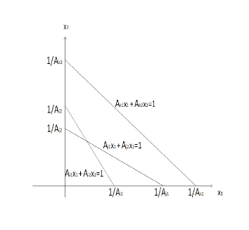
Figure 1: Constraints in Category 1

• Let $L_{1}$ be the number of constraints in this category. We find the smallest intercept in x-axis $[ix,{i}]=\min_{i}\left\{\frac{1}{A_{i1}}\right\}$ and the smallest intercept in y-axis $[iy,{j}]=\min_{i}\left\{\frac{1}{A_{i2}}\right\}$.

• If ${i}={j}$, all constraints except ${i}$th constraint are redundant. Denote the candidate non-redundant constraint set $C_{1}=\{{i}\}$.

• If ${i}\neq{j}$, solving the linear system composed of ${i}$th and ${j}$th equations gives $(x_{1},x_{2})$. Set the candidate non-redundant constraint set $C_{1}=\{{i},{j}\}$.

• For $k=1:L_{1}$

  • If $A_{k1}x_{1}+A_{k2}x_{2}>1$, add index $k$ into candidate non-redundant constraint set $C_{1}$. Otherwise, the $k$th constraint is redundant.

• End (For)

Category 2: $A_{i1}>0$ and $A_{i2}<0$

For constraints in this category, the non-redundant constraints are selected as follows (see Figure 2):

Figure 2: Constraints in Category 2

• Let $L_{2}$ be the number of constraints in this category.

• If $L_{2}=1$ and the only constraint in this category has index $i$, set the candidate non-redundant constraint set $C_{2}=\{i\}$

• Else if $L_{2}>1$

  • Sort $\{\frac{1}{A_{i1}}\}$ in ascending order to get ${\bf s}_{1}=\{\frac{1}{a_{i1}}\}$. Let ${\bf s}_{2}=\{\lvert\frac{a_{i1}}{a_{i2}}\rvert\}$ be obtained by re-arranging $\{\lvert\frac{A_{i1}}{A_{i2}}\rvert\}$ in the same order as ${\bf s}_{1}$. Denote ${\bf S}=[{\bf s}_{1},{\bf s}_{2}]$ and set $j=1$. Let $L$ be the number of rows of ${\bf S}$ and initial candidate non-redundant constraint set $C_{2}$ include the indexes of all rows in ${\bf S}$.

  • While $j<L$

    • Remove all rows in ${\bf S}$ that meet the condition ${\bf S}(i,2)<{\bf S}(j,2)$ and all corresponding indexes $i$ from $C_{2}$.

    • Let $L$ be the number of rows of the reduced matrix ${\bf S}$ and set $j=j+1$.

  • End (While)

• End (If)

Category 3: $A_{i1}<0$ and $A_{i2}>0$

For constraints in this category, the non-redundant constraints are selected as follows (see Figure 3):

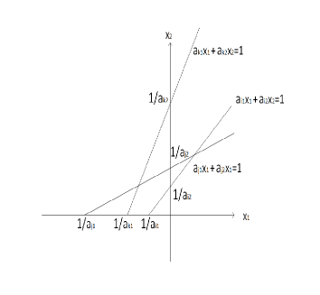
Figure 3: Constraints in Category 3

• Let $L_{3}$ be the number of constraints in this category.

• If $L_{3}=1$ and the only constraint in this category has index $i$, set the candidate non-redundant constraint set $C_{3}=\{i\}$

• Else if $L_{3}>1$

  • Sort $\{\frac{1}{A_{i2}}\}$ in ascending order to get ${\bf s}_{1}=\{\frac{1}{a_{i2}}\}$. Let ${\bf s}_{2}=\{\lvert\frac{a_{i2}}{a_{i1}}\rvert\}$ be obtained by re-arranging $\{\lvert\frac{A_{i2}}{A_{i1}}\rvert\}$ in the same order as ${\bf s}_{1}$. Denote ${\bf S}=[{\bf s}_{1},{\bf s}_{2}]$ and set $j=1$. Let $L$ be the number of rows of ${\bf S}$ and initial candidate non-redundant constraint set $C_{3}$ include the indexes of all rows in ${\bf S}$.

  • While $j<L$

    • Remove all rows in ${\bf S}$ that meet the condition ${\bf S}(i,2)>{\bf S}(j,2)$ and all corresponding indexes $i$ from $C_{3}$.

    • Let $L$ be the number of rows of the reduced matrix ${\bf S}$ and set $j=j+1$.

  • End (While)

• End (If)

Category 4: $A_{i1}>0$ and $A_{i2}=0$

For constraints in this category, we remove all constraints except the $\imath$th constraints satisfying $\frac{1}{A_{\imath 1}}=\min_{i}\frac{1}{A_{i1}}$.

Category 5: $A_{i1}=0$ and $A_{i2}>0$

For constraints in this category, we remove all constraints except the $\imath$th constraints satisfying $\frac{1}{A_{\imath 2}}=\min_{i}\frac{1}{A_{i2}}$.

After removing the redundant constraints as described as above, the number of rows in $\bar{{\bf A}}_{1}$ will be significantly reduced, hence the number of equations expressed in the form of (23) will be significantly reduced.

Both Algorithm 2.1 and Dantzig’s pivot algorithm are implemented in Matlab. Numerical test is carried out for randomly generated problems which are obtained as follows: first, given the problem size $m$, a matrix ${\bf M}$ with random entries of dimension $m\times m$ and an identity matrix of dimension $m$ are generated. ${\bf A}=[{\bf M}~{}~{}~{}{\bf I}]$ is determined whose initial basic solution is composed of the last $m$ columns. Then a positive vector ${\bf b}$ with random entries of dimension $m$ and a vector ${\bf c}=({\bf c}_{1},{\bf 0})$ with ${\bf c}_{1}$ a random vector of dimension $m$ are generated. For each of these LP problems, Dantzig’s pivot algorithm and the double-pivot algorithm are used to solve the LP problem. For each given problem size $m$, this test is repeated for $100$ randomly generated problems. The average iteration number and average computational time in seconds are obtained. The test results are presented in Table LABEL:table2, It is easy to see that for all problems with different size, the double-pivot algorithm uses few iterations on average than Dantzig’s pivot algorithm. For small size problems, Dantzig’s pivot algorithm uses significant less CPU time than the double-pivot algorithm. As the problem size increases, the double-pivot algorithm becomes more and more competitive to Dantzig’s pivot algorithm. For $m=1000$, the CPU times used by the two algorithms are very close. For $m=2000$, it takes hours of the CPU times for either algorithm to solve a randomly generated dense LP problem. Therefore, the test stops for problems with $m=1000$. According to the trends of the CPU times (and iteration numbers) used by the two algorithms for different problem sizes, we guess that for problems with size $m=10000$ and larger, the double-pivot algorithm will be more efficient than Dantzig’s pivot algorithm.

Table 2: Comparison test for Dantzig pivot and double pivot rules

Problem	Dantzig pivot rule		double pivot rule
size m	iteration	CPU time (s)	iteration	CPU time (s)
10	6.3800	0.0007	4.2200	0.0110
100	160.03	0.0579	155.76	0.2537
1000	17683	1641.1	7512	3097.7

5 Conclusion

In this paper, a double-pivot simplex method is proposed. Two upper bounds of the iteration numbers for the proposed algorithm are derived. The first bound is very tight and attainable. The second bound, when it is applied to some special linear programming problems, such as LP with a totally unimodular matrix and Markov Decision Problem with a fixed discount rate, shows that the double pivot algorithm will find the optimal solution in a strongly polynomial time. The numerical test shows very promising result. It is hoped that the double-pivot strategy may lead to some strongly polynomial algorithms for general linear programming problems.

6 Acknowledgment

This author would like to thank Dr. F. Vitor for sharing his recent paper which is useful in comparing the proposed work and his excellent work.

7 Conflict of interest

On behalf of all authors, the corresponding author states that there is no conflict of interest.

References

- [1] D. Avis and V. Chvàtal, (1978), Notes on Bland’s pivoting rule, Mathematical Programming Study, 8, 24-34.
- [2] N. Bonifas, M.D. Summa, F. Eisenbrand, N. Hahnle, and M. Niemeier, (2014), On sub-determinants and the diameter of polyhedra. Discrete and Computational Geometry, 52, 102-115.
- [3] G.B. Dantzig, (1949), Programming in a linear structure, Econometrica 17, 73-74.
- [4] G.B. Dantzig, (1963), Linear programming and extensions, Princeton University Press, Princeton, 1963.
- [5] O. Friedmann, (2011), A subexponential lower bound for Zadeh’s pivoting rule for solving linear programs and games., In: IPCO, pp. 192-206.
- [6] B. Gartner, M. Henk, and G.M. Ziegler (1998), Randomized simplex algorithms on Klee-Minty cubes, Combinatorica, 18(3), 49-372.
- [7] D. Goldfarb and W.Y. Sit, (1979), Worst case behavior of the steepest edge simplex method, Discrete Applied Mathematics, 1, 277-285.
- [8] H. J. Greenberg, (1997), Klee-Minty polytope shows exponential time complexity of simplex method, University of Colorado at Denver, http://www.cudenver.edu/ hgreenbe.
- [9] F. Ihrahima, (2013), Degeneracy and geometry in the simplex method, Stanford University report, available from the Internet, https://pdfs.semanticscholar.org/0b28/52b085df3288d0ddcc28c5e511082fd03fef.pdf.
- [10] R.G. Jeroslow, (1973), The simplex algorithm with the pivot rule of maximizing criterion improvement, Discrete Mathematics, 4, 367-377.
- [11] G. Kalai and D. Kleitman, (1992), A quasi-polynomial bound for the diameter of graphs of polyhedra, Bulletin of the American Mathematical Society, 26, 315-316.
- [12] J.A. Kelner and D.A. Spielman, (2006), A randomized polynomial-time simplex algorithm for linear programming, Proceedings of the thirty-eighth annual ACM symposium on Theory of Computing, 51-60.
- [13] T. Kitahara and S. Mizuno, (2011), Klee-Minty’s LP and upper bounds for Dantzig’s simplex method, Operations Research Letters, 39(2), 88-91.
- [14] T. Kitahara and S. Mizuno, (2013), A bound for the number of different basic solutions generated by the simplex method, Mathematical Programming, 137, 579-586.
- [15] T. Kitahara and S. Mizuno, (2013) An upper bound for the number of different solutions generated by the primal simplex method with any selection rule of entering variables, Asia-Pacific Journal of operational research, 30, 1340012, [10 pages].
- [16] V. Klee and G.J. Minty, (1972), How good is the simplex algorithm? In O. Shisha, editor, Inequalities, III, 159-175. Academic Press, New York, NY.
- [17] K. Paparrizos, N. Samaras, and D. Zissopoulos, (2008) Linear programming: Klee-Minty examples, In: Floudas C., Pardalos P. (eds) Encyclopedia of Optimization. Springer, Boston, MA
- [18] N. Ploskas and N. Samaras, (2014), Pivoting rules for the revised simplex algorithm, Yugoslav Journal of Operations Research, 24(3), 321-332.
- [19] F. Santos, (2012), A counterexample to the Hirsch conjecture, Annals of Mathematics, 176, 383-412.
- [20] F. Santos, (2012), The Hirsch conjecture has been disproved: An interview with Francisco Santos, EMS Newsletter, December 2012.
- [21] S. Smale, (1999). Mathematical problems for the next century. In Arnold, V. I.; Atiyah, M.; Lax, P.; Mazur, B. Mathematics: frontiers and perspectives, American Mathematical Society, 271-294.
- [22] N. Sukegawa, (2017), Improving bounds on the diameter of a polyhedron in high dimensions, Discrete Mathematics, 340, 2134-2142.
- [23] T. Terlaky and S. Zhang, (1993), Pivot rules for linear programming: A survey on recent theoretical developments, Annals of Operations Research, Vol. 46 (1), 203-233.
- [24] M. J. Todd, (2014), An improved Kalai–Kleitman bound for the diameter of a polyhedron, SIAM Journal on Discrete Mathematics, 26(2), 1944-1947.
- [25] F. Vitor and T. Easton, (2018), The double pivot simplex method, Mathematical Methods of Operations Research, 87(1), 109-137.
- [26] Y. Yang, (2018), On the diameter of polytopes, arXiv:1809.06780v1.
- [27] Y. Ye, (2011), The simplex and policy-iteration methods are strongly polynomial for the Markov decision problem with a fixed discount rate, Mathematics of Operations Research, 36(4), 593-603.