Meta Matrix Factorization for Federated Rating Predictions

Abstract.

Federated recommender systems have distinct advantages in terms of privacy protection over traditional recommender systems that are centralized at a data center. With the widespread use and the growing computing power of mobile devices, it is becoming increasingly feasible to store and process data locally on the devices and to train recommender models in a federated manner. However, previous work on federated recommender systems does not fully account for the limitations in terms of storage, RAM, energy and communication bandwidth in a mobile environment. The scales of the models proposed are too large to be easily run on mobile devices. Also, existing federated recommender systems need to fine-tune recommendation models on each device, which makes it hard to effectively exploit collaborative filtering information among users/devices.

Our goal in this paper is to design a novel federated learning framework for rating prediction (RP) for mobile environments that operates on par with state-of-the-art fully centralized RP methods. To this end, we introduce a federated matrix factorization (MF) framework, named meta matrix factorization (MetaMF), that is able to generate private item embeddings and RP models with a meta network. Given a user, we first obtain a collaborative vector by collecting useful information with a collaborative memory module. Then, we employ a meta recommender module to generate private item embeddings and a RP model based on the collaborative vector in the server. To address the challenge of generating a large number of high-dimensional item embeddings, we devise a rise-dimensional generation strategy that first generates a low-dimensional item embedding matrix and a rise-dimensional matrix, and then multiply them to obtain high-dimensional embeddings. We use the generated model to produce private RPs for the given user on her device.

MetaMF shows a high capacity even with a small RP model, which can adapt to the limitations of a mobile environment. We conduct extensive experiments on four benchmark datasets to compare MetaMF with existing MF methods and find that MetaMF can achieve competitive performance. Moreover, we find MetaMF achieves higher RP performance over existing federated methods by better exploiting collaborative filtering among users/devices.

1. Introduction

Traditionally, recommender systems are organized in a centralized fashion, i.e., service providers hold all data and models at a data center. As even an anonymized centralized dataset still puts user privacy at risk via combinations with other datasets (Sweeney, 2000), federated or decentralized recommender systems are increasingly being considered so to realize privacy-aware recommendations (Ammad-ud din et al., 2019; Barbosa et al., 2018; Wang et al., 2015). In federated recommender systems, a global model in the server can be trained from user-specific local models on multiple mobile devices (e.g., phones, laptops, smartwatches), ensuring that users’ interaction data never leaves their devices. Such recommender systems are capable of reducing the risk of leaking private user data.

Larger recommendation models need more space for storage, more RAM for running programs, more energy for calculation, and more communication bandwidth for downloading or updating. Unlike fully centralized recommender systems at a data center, federated recommender systems that need to run on local devices have stricter requirements on the scale of the model. Previous work on federated recommender systems (Ziegler, 2004; Massa and Avesani, 2007; Wang et al., 2015; Ammad-ud din et al., 2019; Chen et al., 2018a) neglects to fully account for the model scale, so that the proposed federated recommendation approaches need to fine-tune the model on each device. Accordingly, limited device resources (e.g., storage, RAM, energy, and communication bandwidth, etc.) are heavily occupied. Moreover, existing federated approaches cannot effectively exploit collaborative filtering (CF) information among users/device, which limits the performance of existing federated recommendation methods.

To tackle the problems listed above, we focus on a new privacy-aware federated recommendation architecture for the RP task (Marlin, 2004; Koren, 2008; Li and She, 2017). For the RP task we aim to predict the rating that a user would give to an item that she has not rated in the past as precisely as possible (Koren et al., 2009; Hu et al., 2014). In this paper, our target is to design a novel federated learning framework to RP for a federated mobile environment that operates on par with state-of-the-art fully centralized RP methods.

As the method of choice for the RP task, MF is used to optimize latent factors to represent users and items by projecting users and items into a joint dense vector space (Koren et al., 2009; He et al., 2017). Today’s MF methods consider RP models as well as item embeddings of the same size and shared parameters for all users in order to predict personalized ratings. For fitting all user data, the shared RP model with item embeddings must be large in size. In this paper, we hypothesize that using private item embeddings and models can achieve competitive performance with a small model scale, based on two intuitions. First, different users might have different views and/or angles about the same item: it is not necessary for all users to use shared item embeddings that require many parameters. Second, different users might favor different RP strategies, which means we can use a specific and small model to fit a user’s private data. A key challenge is how we can build private RP models on local devices and at the same time effectively utilize collaborative filtering (CF) information on the server as we may not have enough personal data for each user to build her own model.

In this paper, we address this challenge by introducing a novel matrix factorization framework, namely meta matrix factorization (MetaMF). Instead of building a model on each local device, we propose to “generate” private item embeddings and RP models with a meta network. Specifically, we assign a so-called indicator vector (i.e., a one-hot vector corresponding to a user id) to each user. For a given user, we first fuse her indicator vector to get a collaborative vector by collecting useful information from other users with a collaborative memory (CM) module. Then, we employ a meta recommender (MR) module to generate private item embeddings and a RP model based on the collaborative vector. It is challenging to directly generate the item embeddings due to the large number of items and the high dimensions. To tackle this problem, we devise a rise-dimensional generation (RG) strategy that first generates a low-dimensional item embedding matrix and a rise-dimensional matrix, and then multiply them to obtain high-dimensional embeddings. Finally, we use the generated RP model to obtain RPs for this user. In a federated recommender system, we deploy the private RP model on the user’s device, and the meta network, including CM and MR modules, on the server.

We perform extensive experiments on four benchmark datasets. Despite its federated nature, MetaMF shows comparable performance with state-of-the-art MF methods on two datasets, while using fewer parameters for item embeddings and RP models. Both the generated item embeddings and the RP model parameters exhibit clustering phenomena, demonstrating that MetaMF can effectively model CF in a federated manner while generating a private model for each user. Moreover, we find that MetaMF achieves higher RP performance than state-of-the-art federated recommendation methods by better exploiting CF among users/devices. To facilitate reproducibility of the results, we are sharing the code.

The main contributions of this paper are as follows:

• We introduce a novel federated matrix factorization (MF) framework, MetaMF, that can reduce the parameters of RP models and item embeddings without loss in performance.

• We devise a meta network, including collaborative memory and meta recommender modules, to better exploit collaborative filtering in federated recommender systems.

• We propose a rise-dimensional generation strategy to reduce the parameters and calculation in generation.

• We conduct extensive experiments and analyses to verify the effectiveness and efficiency of MetaMF.

2. Related Work

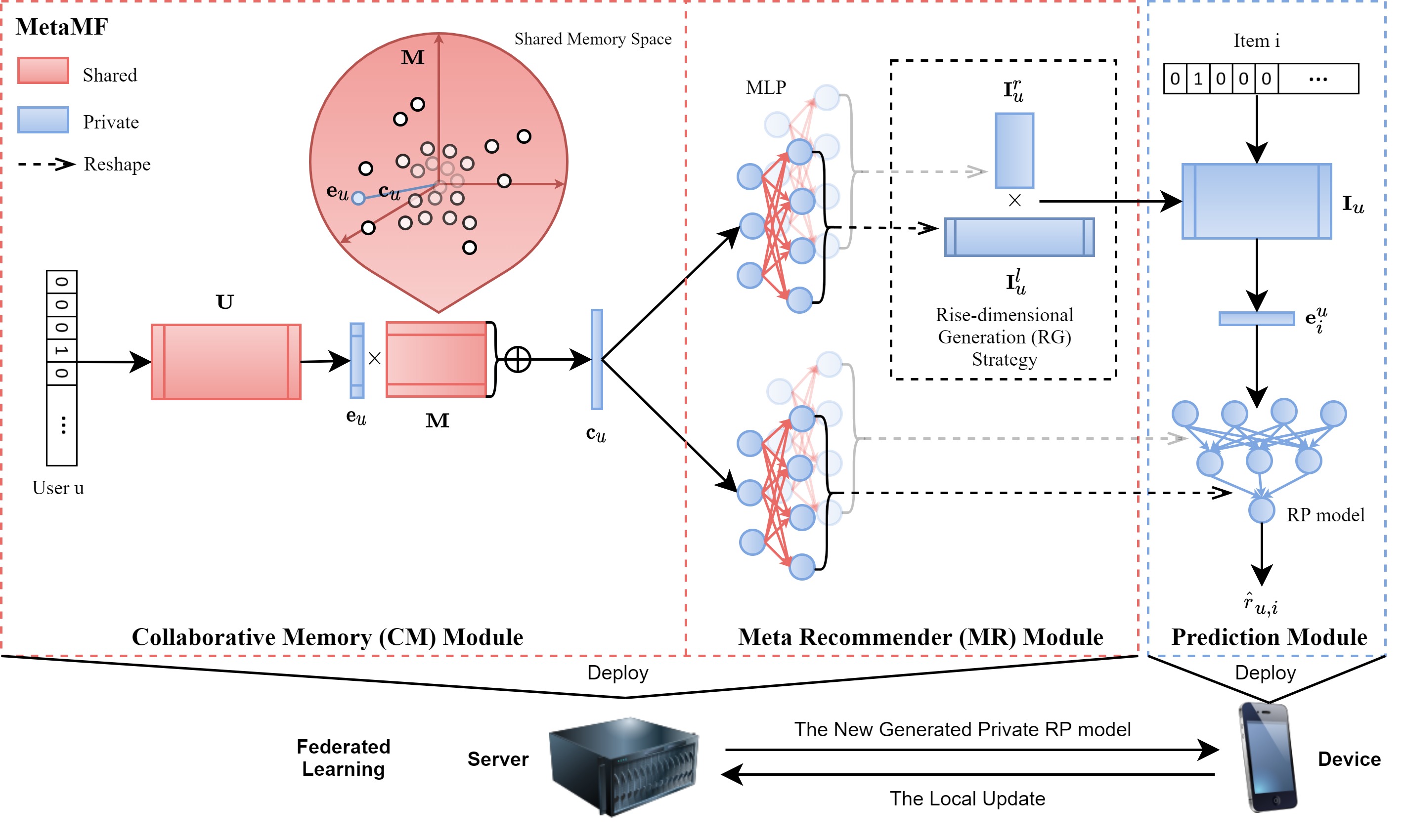
Figure 1. An overview of MetaMF. It consists of three modules. The CM module and the MR module with the RG strategy tend to generate private item embeddings and RP models for different users, which are deployed into the server. The prediction module aims to predict private ratings based on the generated item embeddings and RP models for each user, which is deployed into the device.

We group related work into federated recommender systems, matrix factorization, and meta learning.

2.1. Federated Recommender Systems

For RPs in a federated environment, it is impractical to only rely on local data to train a model for each device, due to data sparsity. Thus, previous work for the federated environment focuses on how to collaboratively train models on distributed data using existing recommendation methods. Ziegler (2004) propose to build a graph among computers based on trust, then to use collaborative filtering to do recommendations. Kermarrec et al. (2010) further present a user-based random walk approach with CF across devices to predict ratings. Wang et al. (2015) introduce a parallel and distributed matrix factorization algorithms to cooperatively learn user/item latent factors across multiple devices. Barbosa et al. (2018) propose that smartphones exchange data between devices and calculate their own recommendation via collaborative filtering. Beierle and Eichinger (2019) further present a mobile architecture consisting of data collection, data exchange, and a local recommender system; the data collection component gets data about the user from local device, data exchange gets data about other users from other devices, and the local recommender system utilizes all available data for recommending items to the user.

Several studies have introduced federated learning (McMahan et al., 2017) into the realm of recommendation, which provides a way to realize federated recommender systems. Chen et al. (2018a) propose a recommendation framework based on federated meta learning, which maintains a shared model in the cloud. To adapt it for each user, they download the model to the local device and fine-tune the model for personalized recommendations. Ammad-ud din et al. (2019) formulate federated collaborative filtering (FCF) methods and adapt WRMF (Hu et al., 2008) to demonstrate the applicability of FCF.

Unlike us, Ammad-ud din et al. (2019) do not focus on the size of the local models while maintaining performance; importantly, they focus on the ranking task, not the rating prediction task that we focus on. In previous federated learning methods, the global model in the server and the local model in the device have the same size, the local model is a copy of the global model. No previous work uses the type of architecture that we design for MetaMF that deploys a big meta network into the server to exploit CF while deploying a small RP model into the device to predict ratings.

2.2. Matrix Factorization

Matrix factorization (MF) has attracted a lot of attention since it was proposed for recommendation tasks. Early studies focus mainly on how to achieve better rating matrix decomposition. Sarwar et al. (2000) employ singular value decomposition (SVD) to reduce the dimensionality of the rating matrix, so that they can get low-dimensional user and item vectors. Goldberg et al. (2001) apply principal component analysis (PCA) to decompose the rating matrix, and obtain the principal components as user or item vectors. Zhang et al. (2006) propose non-negative matrix factorization (NMF), which decomposes the rating matrix by modeling each user’s ratings as an additive mixture of rating profiles from user communities or interest groups and constraining the factorization to have non-negative entries. Mnih and Salakhutdinov (2008) propose probabilistic matrix factorization (PMF) to model the distributions of user and item vectors from a probabilistic point of view. Koren (2008) proposes SVD++, which enhances SVD by including implicit feedback as opposed to SVD, which only includes explicit feedback.

The matrix decomposition methods mentioned above estimate ratings by simply calculating the inner product between user and item vectors, which is not sufficient to capture their complex interactions. Deep learning has been introduced to MF to better model user-item interactions with non-linear transformations. Sedhain et al. (2015) propose AutoRec, which takes ratings as input and reconstructs the ratings by an autoencoder. Later, Strub et al. (2016) enhance AutoRec by incorporating side information into a denoising autoencoder. He et al. (2017) propose the neural collaborative filtering (NCF), which employs a multi-layer perceptron (MLP) to model user-item interactions. Xue et al. (2017) present the deep matrix factorization (DMF) which enhances NCF by considering both explicit and implicit feedback. He et al. (2018) use convolutional neural networks to improve NCF and present the ConvNCF, which uses the outer product to model user-item interactions. Cheng et al. (2018) introduce an attention mechanism into NCF to differentiate the importance of different user-item interactions. Recently, a number of studies have investigated the use of side information or implicit feedback to enhance these neural models (Li and She, 2017; Xiao et al., 2019a, b; Yi et al., 2019).

All these models provide personalized RPs by learning user representations to encode differences among users, while sharing item embeddings and models. In contrast, MetaMF provides private RPs by generating non-shared and small models as well as item embeddings for individual users.

2.3. Meta Learning

Meta learning, also known as “learning to learn,” has shown its effectiveness in reinforcement learning (Xu et al., 2018), few-shot learning (Nichol et al., 2018), image classification (Ravi and Larochelle, 2017).

Jia et al. (2016) propose a network to dynamically generate filters for CNNs. Bertinetto et al. (2016) introduce a model to predict the parameters of a pupil network from a single exemplar for one-shot learning. Ha et al. (2016) propose hypernetworks, which employ a network to generate the weights of another network. Krueger et al. (2017) present a Bayesian variant of hypernetworks that learns the distribution over the parameters of another network. Chen et al. (2018b) use a hypernetwork to share function-level information across multiple tasks. Few of them target recommendation, which is a more complex task with its own unique challenges.

Recently, some studies have introduced meta learning into recommendations. Vartak et al. (2017) study the item cold-start problem in recommendations from a meta learning perspective. They view recommendation as a binary classification problem, where the class labels indicate whether the user engaged with the item. Then they devise a classifier by adapting a few-shot learning paradigm (Snell et al., 2017). Lee et al. (2019) propose a meta learning-based recommender system called MeLU to alleviate the user cold-start problem. MeLU can estimate new users’ preferences with a few consumed items and determine distinguishing items for customized preference estimation by an evidence candidate selection strategy. Du et al. (2019) unify scenario-specific learning and model-agnostic sequential meta learning into an integrated end-to-end framework, namely Scenario-specific Sequential Meta learner (s²Meta). s²Meta can produce a generic initial model by aggregating contextual information from a variety of prediction tasks and effectively adapt to specific tasks by leveraging learning-to-learn knowledge.

Different from these publications, we learn a hypernetwork (i.e., MetaMF) to directly generate private MF models for each user for RPs.

3. Meta Matrix Factorization

3.1. Overview

Given a user $u$ and an item $i$, the goal of rating prediction (RP) is to estimate a rating $\hat{r}_{u,i}$ that is as accurate as the true rating $r_{u,i}$. We denote the set of users as $\mathcal{U}$, the set of items as $\mathcal{I}$, the set of true ratings as $\mathcal{R}$, which will be divided into the training set $D_{train}$, the validation set $D_{valid}$, and the test set $D_{test}$.

As shown in Fig. 1, MetaMF has three components: a collaborative memory module (see Section 3.3), a meta recommender module (see Section 3.4 and a prediction module (i.e., a RP model; see Section 3.5), where the CM and MR modules constitute a meta network shared by all users, and the prediction module is private. In CM module, we first obtain the user embedding $\mathbf{e}_{u}$ of $u$ from the user embedding matrix $\mathbf{U}$ and take it as the coordinates to obtain the collaborative vector $\mathbf{c}_{u}$ from a shared memory space that fuses information from all users. Then we input $\mathbf{c}_{u}$ to the MR module to generate the parameters of a private RP model for $u$. The RP model can be of any type. In this work, the RP model is a multi-layer perceptron (MLP). We also generate the private item embedding matrix $\mathbf{I}_{u}$ of $u$ with a rise-dimensional generation strategy. Finally, the prediction module takes the item embedding $\mathbf{e}_{ui}$ of $i$ from $\mathbf{I}_{u}$ as input and predicts $r_{u,i}$ using the generated RP model.

3.2. Federated Rating Predictions

Before we detail each module, we first detail how to use MetaMF to decentralize data to build a federated recommender system. Because MetaMF can be divided into a meta network, including CM and MR modules, and a RP model, i.e., the prediction module, making it suitable to combine with federated learning to realize a federated recommender system.

Specifically, we can deploy the CM and MR modules into a data center, i.e., the server, and deploy the prediction module locally into mobile devices. The centralized server first generates and delivers different parameters to different mobile devices. Next, each mobile device calculates the loss and the gradients of the parameters in the prediction module based on its private data, and uploads the gradients to the server. Then the server can calculate the gradients of the parameters in the CM and MR modules based on the gradients gathered from each device, and update the parameters. Finally, the server generates and delivers new parameters to each mobile device. Like federated machine learning methods, MetaMF can protect user privacy to a certain extent, because user data does not need to be uploaded to the server. Naturally, the strength of the privacy protection depends on the content of the updates; see Section 7.

MetaMF provides a solid trade-off between exploiting CF for higher RP performance and protecting users’ personal information. It places the meta network with the most parameters in the server and places the prediction module of a small scale in devices, which is more suitable to a mobile environment with limited storage, RAM, energy and communication bandwidth.

3.3. Collaborative Memory Module

In order to facilitate collaborative filtering, we propose the CM module to learn a collaborative vector for each user, which encodes both the user’s own information and some useful information from other users.

Specifically, we assign each user $u$ and each item $i$ the indicator vectors, $\mathbf{i}_{u}\in\mathbb{R}^{m}$ and $\mathbf{i}_{i}\in\mathbb{R}^{n}$ respectively, where $m$ is the number of users and $n$ is the number of items. Note that $\mathbf{i}_{u}$ and $\mathbf{i}_{i}$ are one-hot vectors with each dimension corresponding to a particular user or item. For the given user $u$, we first get the user embedding $\mathbf{e}_{u}$ by Eq. 1:

(1) $$\mathbf{e}_{u}=\mathbf{U}\mathbf{i}_{u},$$

where $\mathbf{e}_{u}\in\mathbb{R}^{d_{u}}$, $\mathbf{U}\in\mathbb{R}^{d_{u}\times{m}}$ is the user embedding matrix, and $d_{u}$ is the size of user embeddings. Then we proceed to obtain a collaborative vector for $u$. Specifically, we use a shared memory matrix $\mathbf{M}\in\mathbb{R}^{d_{u}\times{k}}$ to store the basis vectors which span a space of all collaborative vectors, where $k$ is the dimension of basis vectors and collaborative vectors. And we consider the user embedding $\mathbf{e}_{u}$ as the coordinates of $u$ in the shared memory space. So the collaborative vector $\mathbf{c}_{u}\in\mathbb{R}^{k}$ for $u$ is a linear combination of the basis vectors in $\mathbf{M}$ by $\mathbf{e}_{u}$, as shown in Eq. 2:

(2) $$\mathbf{c}_{u}=\sum_{i}\mathbf{M}(i,:)\mathbf{e}_{u}(i),$$

where $\mathbf{M}(i,:)$ is the $i$-th vector of $\mathbf{M}$ and $\mathbf{e}_{u}(i)$ is the $i$-th scalar of $\mathbf{e}_{u}$. Because the memory matrix $\mathbf{M}$ is shared among all users, the shared memory space will fuse information from all users. MetaMF can flexibly exploit collaborative filtering among users by assigning them with similar collaborative vectors in the space defined by $\mathbf{M}$, which is equivalent to learning similar user embeddings as in existing MF methods.

3.4. Meta Recommender Module

We propose the MR module to generate the private item embeddings and RP model based on the collaborative vector from the CM module.

3.4.1. Private Item Embeddings.

We propose to generate the private item embedding matrix $\mathbf{I}_{u}\in\mathbb{R}^{d_{i}\times{n}}$ for each user $u$, where $d_{i}$ is the size of item embeddings. However, it is a challenge to directly generate the whole item embedding matrix when there are a large number of items with relatively high-dimensional item embeddings (instead of extremely small ones). Therefore, we propose a rise-dimensional generation (RG) strategy to decompose the generation into two parts: a low-dimensional item embedding matrix $\mathbf{I}^{l}_{u}\in\mathbb{R}^{s\times{n}}$ and a rise-dimensional matrix $\mathbf{I}^{r}_{u}\in\mathbb{R}^{d_{i}\times{s}}$, where $s$ is the size of low-dimensional item embeddings and $s\ll d_{i}$. Specifically, we first follow Eq. LABEL:I_l_r to generate $\mathbf{I}^{l}_{u}\in\mathbb{R}^{sn}$ and $\mathbf{I}^{r}_{u}\in\mathbb{R}^{d_{i}s}$ (in the form of vectors):

(3) $$\begin{split}&\mathbf{h}^{l}_{i}=\mathrm{ReLU}(\mathbf{W}^{l}_{i}\mathbf{c}_{u}+\mathbf{b}^{l}_{i}),\quad\mathbf{I}^{l}_{u}=\mathbf{U}^{l}_{i}\mathbf{h}^{l}_{i},\\ &\mathbf{h}^{r}_{i}=\mathrm{ReLU}(\mathbf{W}^{r}_{i}\mathbf{c}_{u}+\mathbf{b}^{r}_{i}),\quad\mathbf{I}^{r}_{u}=\mathbf{U}^{r}_{i}\mathbf{h}^{r}_{i},\end{split}$$

where $\mathbf{W}^{l}_{i}$ and $\mathbf{W}^{r}_{i}\in\mathbb{R}^{o\times{k}}$, $\mathbf{U}^{l}_{i}\in\mathbb{R}^{sn\times{o}}$ and $\mathbf{U}^{r}_{i}\in\mathbb{R}^{d_{i}s\times{o}}$ are weights; $\mathbf{b}^{l}_{i}$ and $\mathbf{b}^{r}_{i}\in\mathbb{R}^{o}$ are biases; $\mathbf{h}^{l}_{i}$ and $\mathbf{h}^{r}_{i}\in\mathbb{R}^{o}$ are hidden states; $o$ is the hidden size. Then we reshape $\mathbf{I}^{l}_{u}$ to a matrix whose shape is $s\times{n}$, and reshape $\mathbf{I}^{r}_{u}$ to a matrix whose shape is $d_{i}\times{s}$. Finally, we multiply $\mathbf{I}^{l}_{u}$ and $\mathbf{I}^{r}_{u}$ to get $\mathbf{I}_{u}$:

(4) $$\mathbf{I}_{u}=\mathbf{I}^{r}_{u}\mathbf{I}^{l}_{u}.$$

Compared to directly generating $\mathbf{I}_{u}$, which needs $O(d_{i}\times{n})$ parameters, the RG strategy needs $O(s\times{n}+d_{i}\times{s})$ parameters which reduces the cost of generating $\mathbf{I}_{u}$. For different users, the generated item embedding matrices are different.

3.4.2. Private RP Model.

We also propose to generate a private RP model for each user $u$. We use a MLP as the RP model, so we need to generate the weights and biases for each layer of MLP. Specifically, for layer $l$, we denote its weights and biases as $\mathbf{W}^{u}_{l}\in\mathbb{R}^{f_{\mathit{out}}\times{f_{\mathit{in}}}}$ and $\mathbf{b}^{u}_{l}\in\mathbb{R}^{f_{\mathit{out}}}$ respectively, where $f_{\mathit{in}}$ is the size of its input and $f_{\mathit{out}}$ is the size of its output. Then $\mathbf{W}^{u}_{l}$ and $\mathbf{b}^{u}_{l}$ are calculated as follows:

(5) $$\begin{split}\mathbf{h}_{g}={}&\mathrm{ReLU}(\mathbf{W}^{h}_{g}\mathbf{c}_{u}+\mathbf{b}^{h}_{g}),\\ \mathbf{W}^{u}_{l}={}&\mathbf{U}^{w}_{g}\mathbf{h}_{g}+\mathbf{b}^{w}_{g},\\ \mathbf{b}^{u}_{l}={}&\mathbf{U}^{b}_{g}\mathbf{h}_{g}+\mathbf{b}^{b}_{g},\end{split}$$

where $\mathbf{W}^{h}_{g}\in\mathbb{R}^{o\times{k}}$, $\mathbf{U}^{w}_{g}\in\mathbb{R}^{f_{\mathit{out}}f_{in}\times{o}}$ and $\mathbf{U}^{b}_{g}\in\mathbb{R}^{f_{\mathit{out}}\times{o}}$ are weights; $\mathbf{b}^{h}_{g}\in\mathbb{R}^{o}$, $\mathbf{b}^{w}_{g}\in\mathbb{R}^{f_{\mathit{out}}f_{\mathit{in}}}$ and $\mathbf{b}^{b}_{g}\in\mathbb{R}^{f_{\mathit{out}}}$ are biases; $\mathbf{h}_{g}\in\mathbb{R}^{o}$ is hidden state. Finally, we reshape $\mathbf{W}^{u}_{l}$ to a matrix whose shape is $f_{\mathit{out}}\times{f_{\mathit{in}}}$. Note that $\mathbf{W}^{h}_{g}$, $\mathbf{b}^{h}_{g}$, $\mathbf{U}^{w}_{g}$, $\mathbf{b}^{w}_{g}$, $\mathbf{U}^{b}_{g}$ and $\mathbf{b}^{b}_{g}$ are not shared by different layers of the RP model. And $f_{\mathit{in}}$ and $f_{\mathit{out}}$ also vary with different layers. Detailed settings can be found in the experimental setup. Also, MetaMF returns different parameters of the MLP to each user.

3.5. Prediction Module

The prediction module estimates the user’s rating for a given item $i$ using the generated item embedding matrix $\mathbf{I}_{u}$ and RP model from the MR module.

First, we get the private item embedding $\mathbf{e}^{u}_{i}\in\mathbb{R}^{d_{i}}$ of $i$ from $\mathbf{I}_{u}$ by Eq. 6:

(6) $$\mathbf{e}^{u}_{i}=\mathbf{I}_{u}\mathbf{i}_{i}.$$

Then we follow Eq. 7 to predict $r_{u,i}$ based on the RP model:

(7) $$\begin{split}\mathbf{h}_{1}={}&\mathrm{ReLU}(\mathbf{W}^{u}_{1}\mathbf{e}^{u}_{i}+\mathbf{b}^{u}_{1}),\\ \mathbf{h}_{2}={}&\mathrm{ReLU}(\mathbf{W}^{u}_{2}\mathbf{h}_{1}+\mathbf{b}^{u}_{2}),\\ \vdots\makebox[5.54826pt]{}&\\ \mathbf{h}_{L-1}={}&\mathrm{ReLU}(\mathbf{W}^{u}_{L-1}\mathbf{h}_{L-2}+\mathbf{b}^{u}_{L-1}),\\ \hat{r}_{u,i}={}&\mathbf{W}^{u}_{L}\mathbf{h}_{L-1}+\mathbf{b}^{u}_{L},\end{split}$$

where $L$ is the number of layers of the RP model. The weights $\{\mathbf{W}^{u}_{1},\mathbf{W}^{u}_{2},\ldots,\mathbf{W}^{u}_{L-1},\mathbf{W}^{u}_{L}\}$ and biases $\{\mathbf{b}^{u}_{1},\mathbf{b}^{u}_{2},\ldots,\mathbf{b}^{u}_{L-1},\mathbf{b}^{u}_{L}\}$ are generated by the MR module. The last layer $L$ is the output layer, which returns a scalar as the predicted rating $\hat{r}_{u,i}$.

3.6. Loss

In order to learn MetaMF, we formulate the RP task as a regression problem and the loss function is defined as:

(8) $$L_{\mathit{rp}}=\frac{1}{|D_{\mathit{train}}|}\sum_{r_{u,i}\in{D_{\mathit{train}}}}(r_{u,i}-\hat{r}_{u,i})^{2}.$$

To avoid overfitting, we add the L2 regularization term:

(9) $$L_{\mathit{reg}}=\frac{1}{2}\|\Theta\|^{2}_{2},$$

where $\Theta$ represents the trainable parameters of MetaMF. Note that unlike existing MF methods, the item embeddings and the parameters of RP models are not included in $\Theta$, because they are also the outputs of MetaMF, not trainable parameters.

The final loss $L$ is a linear combination of $L_{\mathit{rp}}$ and $L_{\mathit{reg}}$:

(10) $$L=L_{\mathit{rp}}+\lambda L_{\mathit{reg}},$$

where $\lambda$ is the weight of $L_{\mathit{reg}}$. The whole framework of MetaMF can be efficiently trained using back propagation with federated learning on decentralized data, as showed in Algorithm 1.

Algorithm 1 MetaMF

1:All trainable parameters $\Theta$, which are stored in the server; The user set $\mathcal{U}$, where one user per device; For user $u$, her local data $D_{u}$ stored in her device, and $D_{\mathit{train}}=\sum_{u\in\mathcal{U}}D_{u}$; ^† means the code is executed in the device.

2:$\Theta$; For user $u$, the parameters of her RP model and item embeddings $\Phi_{u}$, which are stored in her device;

3:Initialize $\Theta$ randomly in the server;

4:for u in $\mathcal{U}$ do

5:     Generate $\Phi_{u}$ based on $\Theta$;

6:     Send $\Phi_{u}$ to $u$’s device;

7:end for

8:while not convergent do

9:     Sample a batch $S$ from $\mathcal{U}$;

10:     for $u$ in $S$ do

11:         Sample a batch $B_{u}$ from $D_{u}$;^†

12:         Calculate the gradient of $\Phi_{u}$ based on $B_{u}$;^†

13:         Upload the gradient to the server;^†

14:         Calculate the gradient of $\Theta$ based on the gradient of $\Phi_{u}$;

15:     end for

16:     Accumulate the gradients of $\Theta$ gathered from $S$;

17:     Update $\Theta$ based on the accumulated gradient;

18:     for u in $\mathcal{U}$ do

19:         Regenerate $\Phi_{u}$ based on new $\Theta$;

20:         Send $\Phi_{u}$ to $u$’s device;

21:     end for

22:end while

4. Experimental Setup

Table 1. Statistics of the datasets, where #avg means the average number of user ratings, Hetrec-ML is the short name of Hetrec-movielens.

Datasets	#users	#items	#ratings	#avg	#sparsity (%)
Douban	2,509	39,576	894,887	357	0.9
Hetrec-ML	2,113	10,109	855,599	405	4.00
Movielens1M	6,040	3,706	1,000,209	166	4.5
Ciao	7,375	105,096	282,619	38	0.04

Table 2. Comparison results of MetaMF and baselines on the four datasets. A superscript ^≈ indicates that there is no statistically significant difference between MetaMF and NCF (two-sided paired t-test, $p<0.01$).

Method	Douban		Hetrec-movielens		Movielens1M		Ciao
	MAE	MSE	MAE	MSE	MAE	MSE	MAE	MSE
NMF	0.602	0.585	0.625	0.676	0.727	0.848	0.750	1.039
PMF	0.639	0.701	0.617	0.644	0.703	0.788	1.501	3.970
SVD++	0.593	0.570	0.579	0.590	0.671	0.740	0.738	0.963
LLORMA	0.610	0.623	0.588	0.603	0.675	0.748	1.349	3.396
RBM	1.058	1.749	1.124	1.947	1.122	2.078	1.132	2.091
AutoRec-U	0.709	0.911	0.660	0.745	0.678	0.775	1.673	5.671
AutoRec-I	0.704	0.804	0.633	0.694	0.663	0.715	0.792	1.038
NCF	0.583	0.547	0.572	0.575	0.675	0.739	0.735	0.937
FedRec	0.760	0.927	0.846	1.265	0.907	1.258	0.865	1.507
MetaMF	0.584≈	0.549	0.571≈	0.578≈	0.687	0.760	0.774	1.043

Table 3. Rating prediction results of MetaMF, MetaMF-SI and MetaMF-SM on the four datasets. MetaMF-SI shares item embeddings for all users; MetaMF-SM shares the parameters of prediction module for all users.

Method	Douban		Hetrec-movielens		Movielens1M		Ciao
	MAE	MSE	MAE	MSE	MAE	MSE	MAE	MSE
MetaMF	0.584	0.549	0.571	0.578	0.687	0.760	0.774	1.043
MetaMF-SI	0.586	0.552	0.590	0.615	0.696	0.784	0.732	0.925
MetaMF-SM	0.595	0.571	0.595	0.622	0.697	0.788	0.789	1.061

We seek to answer the following research questions. (RQ1) How does the proposed method MetaMF for federated rating predictions perform compared to state-of-the-art MF methods for the RP task? Does the federated nature of MetaMF come at cost in terms of performance on the RP task? (RQ2) What is the contribution of generating private item embeddings and RP models?

4.1. Datasets

We conduct experiments on four widely used datasets: Douban (Hu et al., 2014), Hetrec-movielens (Cantador et al., 2011), Movielens1M (Harper and Konstan, 2016) and Ciao (Guo et al., 2014). We list the statistics of these four datasets in Table 1. For each user on each dataset, we randomly separate her data into three chunks: $80\%$ as the training set, $10\%$ as the validation set and $10\%$ as the test set.

4.2. Baselines

We compare MetaMF with the following conventional, deep learning-based and federated MF methods. It is worth noting that in this paper we focus on predicting ratings based on rating matrices, thus for fairness we neglect MF methods that need side information.

• Conventional methods:

  • NMF (Zhang et al., 2006): uses non-negative matrix factorization to decompose rating matrices.

  • PMF (Mnih and Salakhutdinov, 2008): applies Gaussian distributions to model the latent factors of users and items.

  • SVD++ (Koren, 2008): extends SVD by considering implicit feedback for modeling latent factors.

  • LLORMA (Lee et al., 2016): uses a number of low-rank sub-matrices to compose rating matrices.

• Deep learning-based methods:

  • RBM (Salakhutdinov et al., 2007): employs restricted Boltzmann machine (RBM) to model the generation process of ratings.

  • AutoRec (Sedhain et al., 2015): proposes autoencoders to model interactions between users and items. AutoRec has two variants, with one taking users’ ratings as input, denoted by AutoRec-U, and the other taking items’ ratings as input, denoted by AutoRec-I.

  • NCF (He et al., 2017): the state-of-the-art MF method that combines generalized matrix factorization and MLP to model user-item interactions. We adapt NCF for the RP task by dropping the sigmoid activation function on its output layer and replacing its loss function with Eq. 8.

• Federated methods:

  • FedRec (Chen et al., 2018a): a federated recommendation method, which employs MAML (Finn et al., 2017) to learn a shared RP model in the server and update the model for each device. In our experiments, the shared RP model is a MLP with two layers (layer sizes are $16$ and $1$ respectively), and its user/item embedding size is $64$.

4.3. Evaluation Metrics

To evaluate the performance of rating prediction methods, we employ two evaluation metrics, i.e., Mean Absolute Error (MAE) and Mean Square Error (MSE). Both of them are widely applied for the RP task in recommender systems. Given the predicted rating $\hat{r}_{u,i}$ and the true rating $r_{u,i}$ of user $u$ on item $i$ in the test set $D_{\mathit{test}}$, MAE is calculated as:

(11) $$\acs{MAE}=\frac{1}{|D_{\mathit{test}}|}\sum_{r_{u,i}\in{D_{\mathit{test}}}}|r_{u,i}-\hat{r}_{u,i}|.$$

MSE is defined as:

(12) $$\acs{MSE}=\frac{1}{|D_{\mathit{test}}|}\sum_{r_{u,i}\in{D_{\mathit{test}}}}(r_{u,i}-\hat{r}_{u,i})^{2}.$$

Statistical significance of observed differences is tested for using a two-sided paired t-test for significant differences ($p<0.01$).

4.4. Implementation Details

The user embedding size $d_{u}$ and the item embedding size $d_{i}$ are set to $32$. The size of the collaborative vector $k$ is set to $128$. The size of the low-dimensional item embedding $s$ is set to $8$. The hidden size $o$ is set to $512$. And the RP model in the prediction module is an MLP with two layers (one hidden layer and one output layer) whose layer sizes are $8$ and $1$. During training, we initialize all trainable parameters randomly with the Xavier method (Glorot and Bengio, 2010). We choose Adam (Kingma and Ba, 2014) to optimize MetaMF, set the learning rate to $0.0001$, and set the regularizer weight $\lambda$ to $0.001$. Our framework is implemented with Pytorch (Paszke et al., 2019). In our experiments, we implement NCF based on the released code of the author. We use the code released by the respective authors for AutoRec. We use LibRec for the remaining baselines.

5. Experimental Results

5.1. What Is the Cost of Federation?

We start by addressing RQ1 and compare our federated rating prediction model MetaMF with state-of-the-art MF methods. Table 2 lists the RP performance of all MF methods.

Our main observations are as follows. First, on the Douban and Hetrec-movielens datasets, MetaMF outperforms most baselines despite the fact that it is federated while most baselines are centralized. And MetaMF is slightly inferior to NCF, but this difference is not significant. So we can draw the conclusion that the performance of MetaMF is comparable to NCF on these two datasets. See Section 5.2 and Section 6.1 for further analysis.

Second, on the Movielens1M and Ciao datasets, MetaMF does not perform well, in some cases worse than some traditional methods, such as SVD++. The most important reason is that the average numbers of user ratings on these two datasets are small. As shown in Table 1, the statistics #avg on these four datasets are $357$, $405$, $166$ and $38$ respectively. Because the Douban and Hetrec-movielens datasets provide more private data for each user, MetaMF is able to capture the differences among users for learning private item embeddings and RP models. However, the Movielens1M and Ciao datasets lack sufficient data, which limits the performance of MetaMF.

Third and finally, MetaMF significantly outperforms FedRec on all datasets with smaller user/item embedding size and RP model scale. And FedRec performs worse than most baselines on most datasets. The reason may be that FedRec cannot effectively exploit CF information among users/devices. Although FedRec maintains a shared model in the server, it needs to fine-tune the model on each device, which prevents some useful information from being shared among devices. However, MetaMF can flexibly take advantage of CF among users/devices by the meta network. See Section 6.2 for further analysis.

Although federated recommender systems can protect user privacy by keeping data locally, it is harder for them to exploit collaborative filtering among users than for centralized approaches, which affects their performance. So how to share information among multiple devices in a privacy-aware manner is still a core problem in federated recommender systems. We can observe that MetaMF does not outperform NCF, and the performance of FedRec is also worse than of most centralized baselines. Although the federated nature of MetaMF makes it trade performance for privacy, it can still achieve comparable performance with NCF on two datasets, which shows MetaMF can get a better balance between privacy protection and RP performance.

5.2. What Does the Privatization of MetaMF Contribute?

Next we address RQ2 to analyze the effectiveness of generating private item embeddings and RP models to the overall performance of MetaMF. First, we compare MetaMF to MetaMF-SI, which only generates private RP models for different users while sharing a common item embedding matrix among all users. As shown in Table 3, MetaMF outperforms MetaMF-SI on most datasets, except for the Ciao dataset. We conclude that generating private item embeddings for each user can improve the performance of MetaMF. It is possible that the Ciao dataset lacks sufficient private data for learning private item embeddings, so that MetaMF performs worse than MetaMF-SI. And if we compare MetaMF-SI with NCF, we find that MetaMF-SI also outperforms NCF on the Ciao dataset, which indicates that generating private RP models can improve RP on the Ciao dataset.

Next, we compare MetaMF with MetaMF-SM, which generates different item embeddings for different users and shares a common RP model among all users. From Table 3, we can see that MetaMF consistently outperforms MetaMF-SM on all datasets. Thus, generating private RP models for users is able to improve the performance of MetaMF too.

Furthermore, by comparing MetaMF-SI and MetaMF-SM, we observe that MetaMF-SI outperforms MetaMF-SM on all datasets. This shows that item embeddings have a greater impact on the performance of MetaMF than RP models.

Finally, in response to RQ2 we conclude that generating private item embeddings and RP models in MetaMF contributes to overall performance of MetaMF.

6. Analysis

Table 4. The performance of MetaMF with different model scales, where each model scale is represented as a tuple (item embedding size, [layer sizes in the Prediction Module], [collaborative vector size, hidden layer size in the MR Module]).

Model scale	Douban		Hetrec-movielens
	MAE	MSE	MAE	MSE
$(8,[2,1],[32,128])$	0.584	0.548	0.575	0.584
$(16,[4,1],[64,256])$	0.587	0.552	0.573	0.582
$(32,[8,1],[128,512])$	0.584	0.549	0.571	0.578
$(64,[16,1],[256,1024])$	—	—	0.578	0.591

Table 5. The performance of NCF with different model scales, where each model scale is represented as (item embedding size, [layer sizes]).

Model scale	Douban		Hetrec-movielens
	MAE	MSE	MAE	MSE
$(16,[16,8,4,1])$	0.587	0.552	0.585	0.603
$(32,[32,16,8,1])$	0.587	0.552	0.583	0.600
$(64,[64,32,16,1])$	0.584	0.549	0.579	0.595
$(128,[128,64,32,1])$	0.585	0.549	0.574	0.579
$(256,[256,128,64,1])$	0.583	0.547	0.572	0.575
$(512,[512,256,128,1])$	0.584	0.547	0.572	0.581
$(1024,[1024,512,256,1])$	0.586	0.549	0.574	0.582

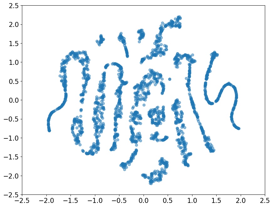
(a) The weights of the hidden layer on the Douban dataset.

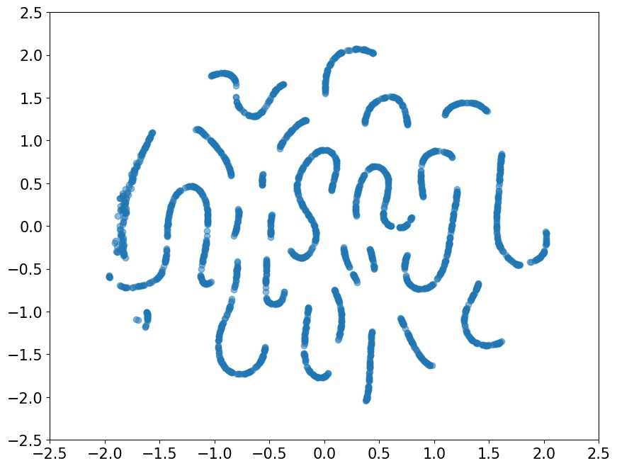
(b) The embeddings of item 16716 on the Douban dataset.

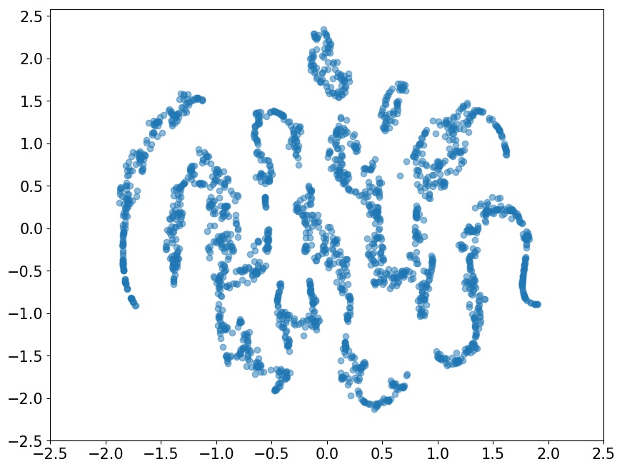
(c) The weights of the hidden layer on the Hetrec-movielens dataset.

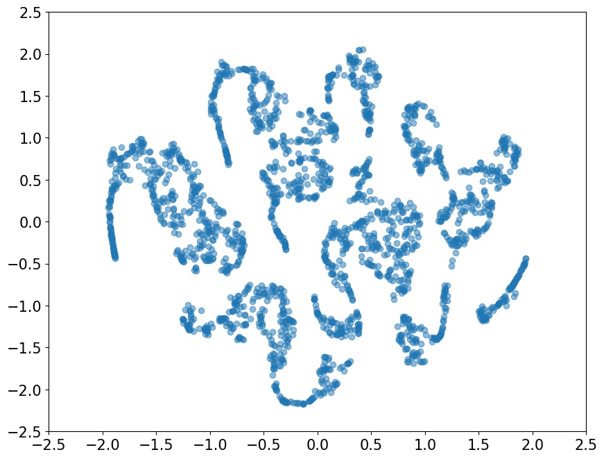
(d) The embeddings of item 1931 on the Hetrec-movielens dataset.

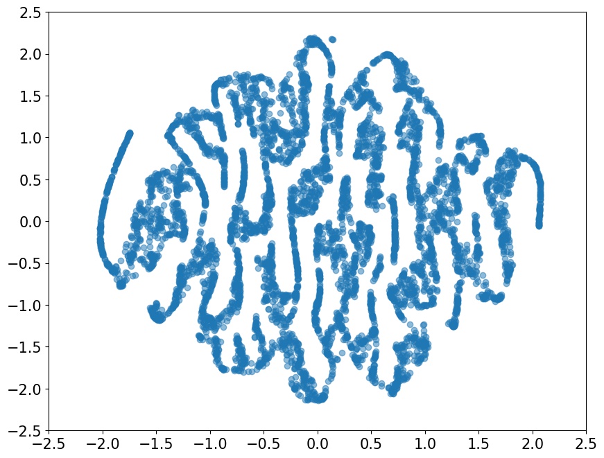
(e) The weights of the hidden layer on the Movielens1M dataset.

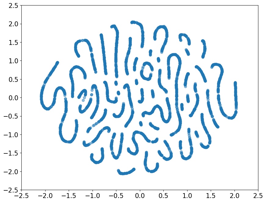
(f) The embeddings of item 482 on the Movielens1M dataset.

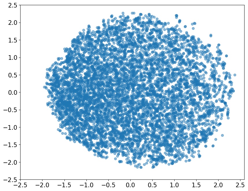
(g) The weights of the hidden layer on the Ciao dataset.

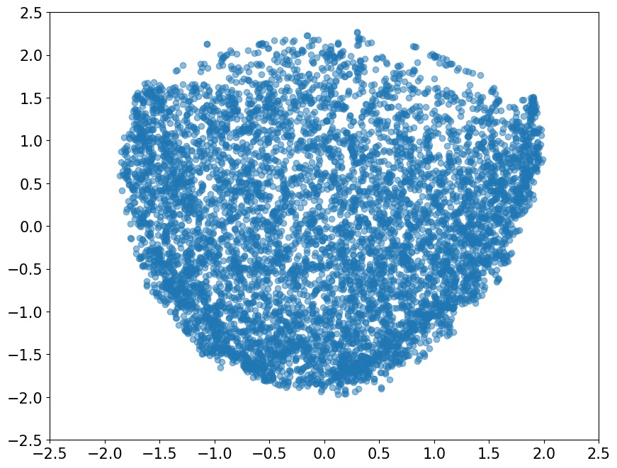
(h) The embeddings of item 8271 on the Ciao dataset.

Figure 2. The generated weights and item embeddings reduced dimension by t-SNE and normalized by mean and standard deviation on the four datasets, where one point corresponds to one user.

Next, we want to understand whether MetaMF shows a high capacity at a small RP model scale compared to NCF. And to which degree does MetaMF generate different item embeddings and RP models for different users while exploiting collaborative filtering?

6.1. Model Scale Analysis

We examine whether MetaMF shows a high model capacity at a small RP model scale by comparing MetaMF with NCF at different model scales on the Douban and Hetrec-movielens datasets. Because MetaMF and NCF are both MLP-based methods, we represent each model scale as a combination of the item embedding size and the list of layer sizes, which are the key hyper-parameters to affect the number of parameters. For MetaMF, we also list the collaborative vector size and the hidden layer size in the CM and MR modules for each model scale, however we only care about the generated parameters in the prediction module of MetaMF because in federated recommender systems we only need to deploy the prediction module (i.e., the RP model) on local devices. Note that the number of parameters we consider is independent from the number of users/devices.

In Table 5 and Table 5, we list the performance of MetaMF and NCF for different model scales. By comparing the best settings of MetaMF $(32,[8],[128,512])$ and NCF $(256,[256,128,64])$, we see that MetaMF achieves a comparable performance with NCF with a smaller item embedding size, fewer layers and smaller layer sizes. Importantly, at small model scales, MetaMF significantly outperforms NCF. This is because the item embeddings and the RP model generated by MetaMF are private, using a small scale is sufficient to accurately encode the preference of a specific user and predict her ratings. However for NCF, the shared RP model with item embeddings has to be large in size since it needs to incorporate the information of all users and predict ratings for all users. We conclude that generating private item embeddings and RP models helps MetaMF to keep a relatively high capacity with fewer parameters in item embeddings and RP models, and improve the performance of rating prediction at the small model scale. Furthermore, when deploying the recommendation system on mobile devices, this advantage of MetaMF can save storage space, RAM, energy and communication bandwidth.

As the model scale increases, the performance of MetaMF deteriorates earlier than NCF. Because there is not sufficient private data to train too many parameters for each user, larger model scales easily lead MetaMF to overfit. And even though we have the RG strategy to alleviate the memory and computational requirements for generating private item embeddings, it is unrealistic to generate larger embeddings for too many items. For example, we do not list the performance of MetaMF with the model scale of $(64,[16],[256,1024])$ on the Douban dataset, because there are too many items in the dataset, making generation too difficult.

6.2. Weights and Embeddings

In order to verify that MetaMF generates private item embeddings and RP models for users while efficiently exploiting CF, we visualize the generated weights and item embeddings after reducing their dimension by t-SNE (van der Maaten and Hinton, 2008) and normalizing them by mean and standard deviation, where each point represents a user’s weights or item embeddings. Because there are many items, we randomly select one item from each dataset for visualization. As shown in Fig. 2, MetaMF generates different weights and item embeddings for different users on most datasets, which indicates that MetaMF has the ability to capture private factors for users. We also notice the existence of many non-trivial clusters in most visualizations, which shows that MetaMF is able to share information among users to take advantage of collaborative filtering in the meta network.

The only exception is on the Ciao dataset, where MetaMF seems unable to learn distinguishable weights and item embeddings. The Ciao dataset does not provide sufficient private data for learning effective weights and item embeddings for each user. It also illustrates why MetaMF does not perform well on the Ciao dataset.

7. Conclusion and Discussion

In this paper, we studied the federated rating prediction problem. In particular, we investigated how to reduce the model scale of matrix factorization methods in order to make them suitable for a federated environment. To achieve this, we proposed a novel matrix factorization framework, named MetaMF, that can generate private RP models as well as item embeddings for each user with a meta network. We conducted extensive experiments to compare and analyze the performance of MetaMF. MetaMF performs competitively, at the level of state-of-the-art RP methods despite using a significant smaller RP model and embedding size for items. In particular, by using collaborative filtering in a federated environment, MetaMF outperforms the federated recommendation method FedRec by a large margin. Thus, we hope MetaMF can advance future research on federated recommendation by presenting a new framework and a scheme.

Next, we discuss some limitations of MetaMF and related future work. First, MetaMF still has a risk of leaking private information. MetaMF uses a meta network to directly generate private item embeddings and RP models on the server. Although the meta network can efficiently exploit CF to improve RP performance, it may leak personal information about users in private item embeddings, RP models and their updates. As future work, we plan to design a more privacy-aware generation network that preserves the high RP performance at the same time. Second, currently MetaMF cannot handle cold-start users well (Bobadilla et al., 2012). Although MetaMF incorporates a CM module to collect collaborative information to alleviate this issue, it still needs a certain amount of data for each user to achieve satisfactory performance. As a result, it does not perform well when there is not enough personalized data for each user. A possible solution direction is to reduce the data requirements of MetaMF using few-shot (Wang and Yao, 2019) or zero-shot learning (Xian et al., 2019). Finally, because the ranking prediction task (Li et al., 2017) is also important in the area of recommendation system, we will also evaluate the performance of MetaMF on the ranking prediction.

Data and Code

To facilitate reproducibility of our work, we are sharing all resources used in this paper at https://github.com/TempSDU/MetaMF.

- (1)
- Ammad-ud din et al. (2019) Muhammad Ammad-ud din, Elena Ivannikova, Suleiman A Khan, Were Oyomno, Qiang Fu, Kuan Eeik Tan, and Adrian Flanagan. 2019. Federated Collaborative Filtering for Privacy-Preserving Personalized Recommendation System. arXiv preprint arXiv:1901.09888 (2019).
- Barbosa et al. (2018) Lucas Nunes Barbosa, Jonathan Gemmell, Miller Horvath, and Tales Heimfarth. 2018. Distributed User-Based Collaborative Filtering on an Opportunistic Network. In AINA. IEEE, 266–273.
- Beierle and Eichinger (2019) Felix Beierle and Tobias Eichinger. 2019. Collaborating with Users in Proximity for Decentralized Mobile Recommender Systems. In UIC. IEEE.
- Bertinetto et al. (2016) Luca Bertinetto, João F Henriques, Jack Valmadre, Philip Torr, and Andrea Vedaldi. 2016. Learning Feed-forward One-shot Learners. In NeurIPS. 523–531.
- Bobadilla et al. (2012) Jesús Bobadilla, Fernando Ortega, Antonio Hernando, and Jesús Bernal. 2012. A Collaborative Filtering Approach to Mitigate the New User Cold Start Problem. Knowledge-based systems 26 (2012), 225–238.
- Cantador et al. (2011) Ivan Cantador, Peter L Brusilovsky, and Tsvi Kuflik. 2011. Second Workshop on Information Heterogeneity and Fusion in Recommender Systems. In HetRec2011.
- Chen et al. (2018a) Fei Chen, Zhenhua Dong, Zhenguo Li, and Xiuqiang He. 2018a. Federated Meta-learning for Recommendation. arXiv preprint arXiv:1802.07876 (2018).
- Chen et al. (2018b) Junkun Chen, Xipeng Qiu, Pengfei Liu, and Xuanjing Huang. 2018b. Meta Multi-task Learning for Sequence Modeling. In AAAI.
- Cheng et al. (2018) Zhiyong Cheng, Ying Ding, Xiangnan He, Lei Zhu, Xuemeng Song, and Mohan S Kankanhalli. 2018. A^ 3NCF: An Adaptive Aspect Attention Model for Rating Prediction. In IJCAI. 3748–3754.
- Du et al. (2019) Zhengxiao Du, Xiaowei Wang, Hongxia Yang, Jingren Zhou, and Jie Tang. 2019. Sequential Scenario-Specific Meta Learner for Online Recommendation. In SIGKDD. ACM.
- Finn et al. (2017) Chelsea Finn, Pieter Abbeel, and Sergey Levine. 2017. Model-agnostic Meta-learning for Fast Adaptation of Deep Networks. In ICML. ACM, 1126–1135.
- Glorot and Bengio (2010) Xavier Glorot and Yoshua Bengio. 2010. Understanding the Difficulty of Training Deep Feedforward Neural Networks. JMLR 9 (2010), 249–256.
- Goldberg et al. (2001) Ken Goldberg, Theresa Roeder, Dhruv Gupta, and Chris Perkins. 2001. Eigentaste: A Constant Time Collaborative Filtering Algorithm. Information retrieval 4, 2 (2001), 133–151.
- Guo et al. (2014) Guibing Guo, Jie Zhang, Daniel Thalmann, and Neil Yorke-Smith. 2014. ETAF: An Extended Trust Antecedents Framework for Trust Prediction. In ASONAM. IEEE, 540–547.
- Ha et al. (2016) David Ha, Andrew Dai, and Quoc V Le. 2016. Hypernetworks. arXiv preprint arXiv:1609.09106 (2016).
- Harper and Konstan (2016) F Maxwell Harper and Joseph A Konstan. 2016. The Movielens Datasets: History and Context. ACM TIIS 5, 4 (2016), 19.
- He et al. (2018) Xiangnan He, Xiaoyu Du, Xiang Wang, Feng Tian, Jinhui Tang, and Tat Seng Chua. 2018. Outer Product-based Neural Collaborative Filtering. In IJCAI.
- He et al. (2017) Xiangnan He, Lizi Liao, Hanwang Zhang, Liqiang Nie, Xia Hu, and Tat-Seng Chua. 2017. Neural Collaborative Filtering. In WWW. ACM, 173–182.
- Hu et al. (2014) Longke Hu, Aixin Sun, and Yong Liu. 2014. Your Neighbors Affect your Ratings: On Geographical Neighborhood Influence to Rating Prediction. In SIGIR. ACM, 345–354.
- Hu et al. (2008) Yifan Hu, Yehuda Koren, and Chris Volinsky. 2008. Collaborative Filtering for Implicit Feedback Datasets. In ICDM. IEEE, 263–272.
- Jia et al. (2016) Xu Jia, Bert De Brabandere, Tinne Tuytelaars, and Luc V Gool. 2016. Dynamic Filter Networks. In NeurIPS. 667–675.
- Kermarrec et al. (2010) Anne-Marie Kermarrec, Vincent Leroy, Afshin Moin, and Christopher Thraves. 2010. Application of Random Walks to Decentralized Recommender Systems. In OPODIS. Springer, 48–63.
- Kingma and Ba (2014) Diederik P Kingma and Jimmy Ba. 2014. Adam: A Method for Stochastic Optimization. arXiv preprint arXiv:1412.6980 (2014).
- Koren (2008) Yehuda Koren. 2008. Factorization Meets the Neighborhood: A Multifaceted Collaborative Filtering Model. In SIGKDD. ACM, 426–434.
- Koren et al. (2009) Yehuda Koren, Robert Bell, and Chris Volinsky. 2009. Matrix Factorization Techniques for Recommender Systems. IEEE Computer 42, 8 (2009), 30–37.
- Krueger et al. (2017) David Krueger, Chin-Wei Huang, Riashat Islam, Ryan Turner, Alexandre Lacoste, and Aaron Courville. 2017. Bayesian Hypernetworks. arXiv preprint arXiv:1710.04759 (2017).
- Lee et al. (2019) Hoyeop Lee, Jinbae Im, Seongwon Jang, Hyunsouk Cho, and Sehee Chung. 2019. MeLU: Meta-Learned User Preference Estimator for Cold-Start Recommendation. In SIGKDD. ACM, 1073–1082.
- Lee et al. (2016) Joonseok Lee, Seungyeon Kim, Guy Lebanon, Yoram Singer, and Samy Bengio. 2016. LLORMA: Local Low-rank Matrix Approximation. JMLR 17, 1 (2016), 442–465.
- Li et al. (2017) Jing Li, Pengjie Ren, Zhumin Chen, Zhaochun Ren, Tao Lian, and Jun Ma. 2017. Neural Attentive Session-based Recommendation. In CIKM. ACM, 1419–1428.
- Li and She (2017) Xiaopeng Li and James She. 2017. Collaborative Variational Autoencoder for Recommender Systems. In SIGKDD. ACM, 305–314.
- Marlin (2004) Benjamin M Marlin. 2004. Modeling User Rating Profiles for Collaborative Filtering. In NeurIPS. 627–634.
- Massa and Avesani (2007) Paolo Massa and Paolo Avesani. 2007. Trust-aware Recommender Systems. In RecSys. ACM, 17–24.
- McMahan et al. (2017) Brendan McMahan, Eider Moore, Daniel Ramage, Seth Hampson, and Blaise Aguera y Arcas. 2017. Communication-Efficient Learning of Deep Networks from Decentralized Data. In AISTATS. 1273–1282.
- Mnih and Salakhutdinov (2008) Andriy Mnih and Ruslan R Salakhutdinov. 2008. Probabilistic Matrix Factorization. In NeurIPS. 1257–1264.
- Nichol et al. (2018) Alex Nichol, Joshua Achiam, and John Schulman. 2018. On First-order Meta-learning Algorithms. arXiv preprint arXiv:1803.02999 (2018).
- Paszke et al. (2019) Adam Paszke, Sam Gross, Francisco Massa, Adam Lerer, James Bradbury, Gregory Chanan, Trevor Killeen, Zeming Lin, Natalia Gimelshein, Luca Antiga, et al. 2019. PyTorch: An Imperative Style, High-performance Deep Learning Library. In NeurIPS. 8024–8035.
- Ravi and Larochelle (2017) Sachin Ravi and Hugo Larochelle. 2017. Optimization as a Model for Few-shot Learning. In ICLR.
- Salakhutdinov et al. (2007) Ruslan Salakhutdinov, Andriy Mnih, and Geoffrey Hinton. 2007. Restricted Boltzmann Machines for Collaborative Filtering. In ICML. ACM, 791–798.
- Sarwar et al. (2000) Badrul Sarwar, George Karypis, Joseph Konstan, and John Riedl. 2000. Application of Dimensionality Reduction in Recommender System – A Case Study. In WebKDD.
- Sedhain et al. (2015) Suvash Sedhain, Aditya Krishna Menon, Scott Sanner, and Lexing Xie. 2015. Autorec: Autoencoders Meet Collaborative Filtering. In WWW. ACM, 111–112.
- Snell et al. (2017) Jake Snell, Kevin Swersky, and Richard Zemel. 2017. Prototypical Networks for Few-shot Learning. In NeurIPS. 4077–4087.
- Strub et al. (2016) Florian Strub, Romaric Gaudel, and Jérémie Mary. 2016. Hybrid Recommender System Based on Autoencoders. In DLRS. ACM, 11–16.
- Sweeney (2000) Latanya Sweeney. 2000. Uniqueness of Simple Demographics in the U.S. Population. Technical Report LIDAP-WP4. Carnegie Mellon University, School of Computer Science, Data Privacy Laboratory, Pittsburgh.
- van der Maaten and Hinton (2008) Laurens van der Maaten and Geoffrey Hinton. 2008. Visualizing Data Using t-SNE. JMLR 9, Nov (2008), 2579–2605.
- Vartak et al. (2017) Manasi Vartak, Arvind Thiagarajan, Conrado Miranda, Jeshua Bratman, and Hugo Larochelle. 2017. A Meta-learning Perspective on Cold-start Recommendations for Items. In NeurIPS. 6904–6914.
- Wang and Yao (2019) Yaqing Wang and Quanming Yao. 2019. Few-shot Learning: A Survey. CoRR (2019).
- Wang et al. (2015) Zhangyang Wang, Xianming Liu, Shiyu Chang, Jiayu Zhou, Guo-Jun Qi, and Thomas S. Huang. 2015. Decentralized Recommender Systems. arXiv preprint arXiv:1503.01647 (2015).
- Xian et al. (2019) Yongqin Xian, Christoph H. Lampert, Bernt Schiele, and Zeynep Akata. 2019. Zero-Shot Learning - A Comprehensive Evaluation of the Good, the Bad and the Ugly. TPAMI 41, 9 (2019), 2251–2265.
- Xiao et al. (2019a) Teng Xiao, Shangsong Liang, Hong Shen, and Zaiqiao Meng. 2019a. Neural Variational Hybrid Collaborative Filtering. In WWW. ACM.
- Xiao et al. (2019b) Teng Xiao, Shangsong Liang, Weizhou Shen, and Zaiqiao Meng. 2019b. Bayesian Deep Collaborative Matrix Factorization. In AAAI.
- Xu et al. (2018) Zhongwen Xu, Hado P van Hasselt, and David Silver. 2018. Meta-gradient Reinforcement Learning. In NeurIPS. 2396–2407.
- Xue et al. (2017) Hong-Jian Xue, Xinyu Dai, Jianbing Zhang, Shujian Huang, and Jiajun Chen. 2017. Deep Matrix Factorization Models for Recommender Systems.. In IJCAI. 3203–3209.
- Yi et al. (2019) Baolin Yi, Xiaoxuan Shen, Hai Liu, Zhaoli Zhang, Wei Zhang, Sannyuya Liu, and Naixue Xiong. 2019. Deep Matrix Factorization with Implicit Feedback Embedding for Recommendation System. IEEE TII (2019).
- Zhang et al. (2006) Sheng Zhang, Weihong Wang, James Ford, and Fillia Makedon. 2006. Learning from Incomplete Ratings Using Non-negative Matrix Factorization. In SDM. SIAM, 549–553.
- Ziegler (2004) Cai-Nicolas Ziegler. 2004. Semantic Web Recommender Systems. In EDBT. Springer, 78–89.