Exact stationary state of a run-and-tumble particle with three internal states in a harmonic trap
Abstract
We study the motion of a one-dimensional run-and-tumble particle with three discrete internal states in the presence of a harmonic trap of stiffness The three internal states, corresponding to positive, negative and zero velocities respectively, evolve following a jump process with rate . We compute the stationary position distribution exactly for arbitrary values of and which turns out to have a finite support on the real line. We show that the distribution undergoes a shape-transition as is changed. For the distribution has a double-concave shape and shows algebraic divergences with an exponent both at the origin and at the boundaries. For the position distribution becomes convex, vanishing at the boundaries and with a single, finite, peak at the origin. We also show that for the special case the distribution shows a logarithmic divergence near the origin while saturating to a constant value at the boundaries.
1 Introduction
Recent years have seen a surge of interest in the study of active matter and active particles. The term ‘active particle’ refers to a class of self-propelled particles which can generate dissipative directed motion by consuming energy directly from their environment [1, 2, 3, 4, 5, 6]. Examples of active matter can be found in nature at all length scales, ranging from micro-organisms like bacteria [7, 8] to granular matter [9, 10], flock of birds [11, 12] and fish-schools [13, 14]. Apart from a diverse set of novel collective behaviours like clustering [15, 16, 17], motility induced phase separation [18, 19, 20], and absence of well defined pressure [21], active particles show many intriguing features even at the single particle level. One such interesting feature is that, in the presence of external potentials and confining boundaries, active particles show very different behaviour than their passive counterparts, including non-Boltzmann stationary state, clustering near the boundaries of the confining region [25, 26, 23, 24, 22] and unusual relaxation and persistence properties [27, 28, 29]. There have been numerous recent studies focusing on the behaviour of active particles in the presence of external potentials and confinements, both theoretical [30, 31, 32, 33] and experimental [34, 35, 36, 37].
The theoretical attempts to characterise the behaviour of active particles focus on studying simple models of such systems. Run-and-tumble particle (RTP) is one of the most studied models of an active particle. An RTP is an overdamped particle which moves with a constant speed , or ‘runs,’ along the direction of an internal ‘spin’ degree of freedom. The orientation of the spin can change randomly resulting in a sudden change, or ‘tumble,’ in the direction of motion of the particle. The simplest example is an RTP moving in one spatial dimension with two possible values of the spin In this case, the particle moves with velocity or the reversal of direction occurs stochastically with rate with the flipping of the spin In the presence of an external potential the position of this two-state RTP evolves according to the Langevin equation,
| (1) |
where is the deterministic force acting on the particle. The spin variable plays the role of the noise, its dichotomous nature giving rise to the ‘activity’. In fact, it is clear from the auto-correlation that is a coloured noise with a finite memory, characterised by the persistence time Despite the apparent simplicity of the model, the two-state RTP shows a lot of intriguing features typical to active particles including non-Boltzmann stationary distribution[24, 27].
For any confining potential, the stationary position distribution of a two-state RTP is known exactly, and is given by,
| (2) |
up to a normalization constant. The above result was first obtained long ago in the context of quantum optics [38, 39, 40, 41], and later to study the role of coloured noise in dynamical systems [42]. More recently, it has been re-derived in the context of active particles [21, 24]. In particular, the stationary distribution (2) has been analysed for specific confining potentials of the type with in Ref. [24]. The case corresponds to a harmonic potential which is of particular interest, not only from theoretical but also from an experimental point of view [35, 37]. For a harmonic potential the stationary distribution (2) simplifies to,
| (3) |
where and is the beta-function. This distribution is symmetric in and has a finite support in the region Consequently, the particle is confined within this region in the stationary state. This stationary position distribution shows an interesting shape-transition as a function of For the distribution is convex shaped, with a peak at the origin and vanishing at the boundaries On the other hand, for has a concave shape with divergences at the boundaries and a minimum at the origin. For the distribution is uniform. Thus by varying one can observe a transition from a double-peaked (at the boundaries) to a single-peaked distribution. The double-peaked nature of the distribution for signifies an ‘active phase’, where the persistence time of the spin-orientation is larger than the relaxation time-scale of the potential. On the other hand, i.e., when the persistence time is smaller compared to corresponds to a passive phase, where the stationary distribution resembles that of a passive particle in a trap, with a single peak at the centre of the trap. Indeed, in the diffusive limit when , but keeping the ratio fixed, the dynamics of the RTP in the harmonic trap converges to the Ornstein-Uhlenbeck process. This is also exhibited in the stationary state where the distribution in Eq. (3) converges to a Boltzmann distribution, which in this case is a simple Gaussian .
It is then natural to ask how the stationary distribution changes if the RTP has more than two internal states. In fact, an RTP with many internal degrees have been studied where the internal degrees can take a set of discrete values and evolve following some discrete jump processes [43, 44]. However, most of these studies are numerical and to the best of our knowledge no analytical results are available for the stationary state of a multi-state RTP in the presence of an external potential.
In this article, we study a run-and-tumble active particle in one spatial dimension with three discrete internal states, with positive, negative and zero velocities, respectively. We show that such a multi-state dynamics naturally arises when one considers an RTP in higher spatial dimensions and project it to one-dimension. We calculate exactly the stationary position probability distribution in the presence of a harmonic potential of strength for arbitrary flip-rate among the internal states. It turns out that the presence of the zero-velocity internal state leads to a rich behaviour of the position distribution . As in the two-state case, it turns out that the shape of the stationary state distribution is governed by one single parameter
| (4) |
We show that has a finite support on the real line and undergoes a transition in shape as is varied : For diverges both at the origin and the boundaries with the same exponent Thus, in this case, the position distribution has a double-concave shape, with three peaks, namely at the boundaries and the origin. For shows a logarithmic divergence near the origin. On the other hand, for the distribution converges to a finite value at the origin while it vanishes at the boundaries, implying a convex shape with a single peak at the origin (see Fig. 2).
2 Model
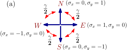
Our model of a three-state RTP in one-dimension is motivated by a natural “clock-like” model for a two-dimensional RTP. Let us indeed consider an overdamped particle moving on a two dimensional plane with an internal orientational degree of freedom or ‘spin’ associated with it. In the absence of any external potential the particle moves with a constant speed along the direction of which is a unit vector with four possible discrete orientations, denoted by (along and axes respectively). The spin evolves in time following a Markov jump process – its orientation can change via a rotation of either clockwise or anti-clockwise, both with rate This jump process is schematically represented in Fig. 1(a). Additionally, we consider an external harmonic potential which exerts a force on the RTP.
The time-evolution of the position of the RTP can be conveniently expressed in terms of the Langevin equations,
| (5a) | |||||
| (5b) | |||||
where are components of the spin vector at any time along the and axes respectively (see Fig. 1(a)).
The position probability distribution is given by the sum where denotes the probability that the particle has the position and orientation at time These probabilities evolve according to the Fokker-Planck (FP) equations,
| (5fa) | |||
| (5fb) | |||
| (5fc) | |||
| (5fd) | |||
where we have suppressed the argument of on the right hand side for the sake of brevity. It is hard to find an analytical form of as these equations are difficult to solve, even in the stationary state.
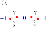
However, it is also interesting to look at the -process only, governed by Eq. (5a). This describes an effective one-dimensional RTP where the internal spin has three possible discrete values, As illustrated in Fig. 1(a), both and correspond to while and corresponds to and respectively. The jump from to can, thus, occur through two different channels ( and ), resulting in a jump rate for Similarly, occurs with rate while occurs with rate (since there is only one way to make this transition). This effective 3-state jump process in one-dimension is schematically shown in Fig. 1(b). Let denote the probability that the RTP is at a position at time with The corresponding FP equations read,
| (5fga) | |||||
| (5fgb) | |||||
| (5fgc) | |||||
We note that this set of FP equations can also be obtained from Eqs. (5fa)-(5fd) by integrating both sides over and then identifying and
In the presence of the confining harmonic potential, in the long time limit the RTP is expected to reach a stationary state where the left hand side (l. h. s.) of the Eqs. (5fga) - (5fgc) would vanish. The corresponding stationary distributions then satisfy a set of coupled linear differential equations (obtained by putting ),
| (5fgha) | |||||
| (5fghb) | |||||
| (5fghc) | |||||
Our objective is to solve this set of equations to find in the stationary state.
Boundary Conditions: To proceed with the solution we first need to specify the boundary conditions for To determine these boundary conditions, we first note that, in the stationary state, the RTP is confined within a finite region bounded by This can be understood easily from the following argument: from the Langevin equation (5a) it is clear that if the particle is outside the region it always feels a drift towards the origin, irrespective of the value of As a result, if the particle starts from some initial position or it will eventually reach the region Consequently, the stationary distribution has a finite support in the region and it is zero outside. To solve Eqs. (5fgha) - (5fghc) then, we need to specify the boundary conditions at these two points. Let us first look at the behaviour of near During an infinitesimal time increment evolves as,
| (5fghi) |
where the first term on the right hand side (r.h.s.) represents the transition when the position of the particle changes by an amount during interval and the second term corresponds to the case when changes from to the pre-factors and denotes the probabilities for these two occurrences, respectively. Now, in the stationary state, the probabilities are independent of time, hence, we have from (5fghi),
| (5fghj) |
Moreover, from Eq. (5a) we have, for and near thus which vanishes in the stationary state, as the argument is outside the region . Then, taking limit in Eq. (5fghj), we get Using similar arguments for and , one finds the full set of boundary conditions to be satisfied by the set of equations (5fgha) - (5fghc),
| (5fghk) |
Note that the behaviour of and remain unspecified. The set of boundary conditions for and is very similar to the case of 2-state RTP [24]. However, as we will see below, the presence of the third state leads to a richer behaviour in the present case.
3 Exact Solution
The straightforward strategy to solve a set of coupled first order equations like Eqs. (5fgha) - (5fghc) is to decouple them and find separate equations for However, our primary goal is to find the marginal position distribution of the particle, i.e., the probability that the effective one-dimensional RTP has a position irrespective of the spin-orientation This is given by
| (5fghl) |
In the following we attempt to derive an equation for using Eqs. (5fgha) - (5fghc). To this end, we first define,
| (5fghm) |
It is straightforward to see that in terms of these functions and , the four boundary conditions given by Eq. (5fghk) translate to,
| (5fghn) |
Note that the boundary conditions of remain unspecified. We proceed by expressing Eqs. (5fgha) - (5fghc) in terms of these functions and For this purpose, we first add equations (5fgha), (5fghb) and (5fghc) to get,
| (5fgho) |
where is a constant independent of To determine we substitute in the above equation. Using the definitions of and along with the boundary condition (5fghk), we get, Hence, from Eq. (5fgho) we have,
| (5fghp) |
for all values of Now, adding Eqs. (5fgha) and (5fghb) and using Eq. (5fghp), we get,
| (5fghq) |
where ′ denotes the derivative with respect to (w.r.t.) the argument of the functions. Next, we subtract Eq. (5fghb) from Eq. (5fgha) to get,
| (5fghr) |
Eqs. (5fghq) and (5fghr) are two coupled linear differential equations involving and In the following, we use them to get two separate differential equations for and But, first, it is convenient to use a change of variable with Let us denote and Eqs. (5fghq) and (5fghr) then become,
| (5fghs) | |||||
| (5fght) |
where The two boundary conditions in Eq. (5fghn) reduce to a single condition for and
| (5fghu) |
As we will see below, this boundary condition is enough to solve the differential equations uniquely.
To get an equation involving only, we take derivative of Eq. (5fghs) w.r.t. Then, using Eq. (5fght), we immediately arrive at a second order differential equation,
| (5fghv) |
It is straightforward to check that the above equation is in the form of a hypergeometric differential equation,
| (5fghw) |
with the parameters,
| (5fghx) |
One can also get a similar second order equation for To this end, we first express in terms of and , i.e., in a form similar to Eq. (5fght). Multiplying Eq. (5fghs) by and Eq. (5fght) by and subtracting the latter resulting equation from the former, we get,
| (5fghy) |
Taking a derivative of Eq. (5fght) and using Eq. (5fghy), we get,
| (5fghz) |
Clearly, this is also a hypergeometric differential equation of the form (5fghw), but with a different parameter set,
| (5fghaa) |
3.1 Position distribution for
The general solutions for Eqs. (5fghv) and (5fghz) can be written in terms of the hypergeometric function [45]. For i.e., for these general solutions read,
| (5fghab) | |||||
| (5fghac) |
where are arbitrary constants. The case is special, which we discuss later. To determine the constants , we first use the original first order equations (5fghs) and (5fght) which must be satisfied by the solution. Substituting Eqs. (5fghab) and (5fghac) in Eq. (5fght) and using well known identities involving the hypergeometric function, we get, and Next, we impose the boundary condition (5fghu). Once again, using properties of hypergeometric functions, we get
| (5fghad) |
To completely specify we still need which can be determined using the normalization condition,
| (5fghae) |
Fortunately, this integral can be performed analytically and yields,
| (5fghaf) |
where denotes the generalized hypergeometric function [45]. Finally, we can write an explicit expression for the stationary position probability distribution,
| (5fghah) | |||||
where the normalization constant is given by Eq. (5fghaf). Note that, is an even function of and it depends on the flip rate comes through the ratio only. takes particularly simple form for certain specific values of
| (5fghal) |
One can also write an explicit expression for using Eqs.(5fghac) and (5fghad),
| (5fghan) | |||||
From Eqs. (5fghah) and (5fghan) and using the relation (5fghp) between and we can also calculate individually in a straightforward manner. However, we do not give explicit expressions for them here.
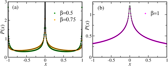
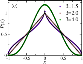
Figure 2(a) and (c) show plots of as a function of for different values of calculated from Eq. (5fghah) along with the data obtained from numerical simulations. It appears that, similar to the 2-state RTP, the distribution shows two different behaviours near the boundary depending on the value of Moreover, it appears from the plots that for also diverges near the origin while it shows a cusp-like behaviour for large In the following we investigate the behaviour of in more details and characterise this change in shape.
Behaviour near : To understand the behaviour of near the origin we use the series expansion of the hypergeometric function near
| (5fghao) |
Using this expansion in Eq. (5fghah), we have, near
| (5fghas) |
where and are given respectively in Eqs. (5fghad) and (5fghaf) while and are given by
| (5fghat) | |||
| (5fghau) |
Clearly, for diverges near the origin whereas for it approaches a finite value. The approach also depends on the value of for has a cusp-like behaviour near the origin while for it shows a quadratic behaviour, resembling a Gaussian around the origin. Indeed, in the diffusive limit, when and keeping fixed (as a consequence in this limit), we find from Eq. (5fghau) that . As a result, from the third line of (5fghas), we recover the Boltzmann distribution which actually holds for all .
Behaviour near : The position distribution also shows an interesting behaviour near the boundaries As is symmetric in it suffices to explore its nature near one boundary, say To characterise the same we use the series expansion of near From Eq. (5fghab), we have, for
| (5fghay) |
Hence, near we have the following behaviour of
| (5fghbc) |
A similar behaviour is seen also near . Note that this “freezing” for the leading behaviour for occurs only for the three-state model, but not for the two-state model [24].
3.2 Position distribution for
As mentioned before, the case is special. In this case, the differential equations (5fghv) and (5fghz) reduce to,
| (5fghbd) | |||
| (5fghbe) |
which correspond to two hypergeometric equations with and along with Eq. (5fghab) is not a general solution anymore as the two hypergeometric functions therein become identical. We use Mathematica to solve Eqs. (5fghbd) and (5fghbe) and it turns out that the general solutions can be expressed in the form,
| (5fghbf) | |||||
| (5fghbg) |
Here is the Legendre’s complete elliptic integral of the first kind (see Ref. [46] and Eq. 19.2.8 in Ref. [45]), is the Meijer’s G-function (see Ref. [46] and Eq. 16.17.1 in Ref. [45]) and is the Legendre function of the second kind (see Eq. 14.3.7 in Ref. [45]).
To determine the arbitrary constants and we use the same strategy as in the previous section. First, we note that the solutions in Eqs. (5fghbf) and (5fghbg) must satisfy the original first order equations (5fghs) and (5fght) with for all values of We then look at the behaviour of and in Eqs. (5fghbf) and (5fghbg) near . In this limit both and diverge logarithmically whereas the Legendre and hypergeometric functions approach a constant value. Substituting the series expansions of these functions back into Eq. (5fght) and comparing coefficients of and different powers of we get, and It is also straightforward to check that Eq. (5fghs) gives the same relation. We still have two independent constants and To determine these we use the boundary condition (5fghu). Using the limiting behaviours of the special functions we have, for which immediately implies [see Eq. (5fghu)]. The last remaining constant can be determined from the normalization condition (5fghae) and yields Finally, we have, for
| (5fghbh) |
Figure 2(b) shows a plot of for together with the same obtained from numerical simulations. To understand the behaviour near the origin and the boundaries we look at the series expansion of Near a logarithmic divergence is seen, On the other hand, near the boundaries approaches a constant value,
4 Conclusion
In this paper, we have solved exactly the stationary position distribution of a one-dimensional run-and-tumble (RTP) particle with three discrete internal states and subjected to an external harmonic potential. To our knowledge, this is the first exact solution with three states that generalizes the well-known result for the standard two-state RTP. We showed that the stationary state exhibits a rich behavior as a function of the single parameter (where represents the rate at which the internal state changes and is the stiffness of the trap). One of the interesting outcomes is that the stationary distribution undergoes a shape-transition at .
While we were able to characterise the stationary state of a three-state RTP in a harmonic trap exactly, it would be interesting to study the relaxational dynamics towards this stationary state, as was recently done for the two-state RTP [24]. It would also be natural to extend our studies to non-harmonic potentials, such as , with . Another natural extension would be to consider an RTP particle with more than internal states. Finding even the stationary state of a general -state RTP with remains a challenging open problem.
References
- [1] P. Romanczuk, M. Bär, W. Ebeling, B. Lindner, and L. Schimansky-Geier, Eur. Phys. J. Special Topics 202, 1 (2012).
- [2] M. C. Marchetti, J. F. Joanny, S. Ramaswamy, T. B. Liverpool, J. Prost, M. Rao, and R. Aditi Simha, Rev. Mod. Phys. 85, 1143 (2013).
- [3] C. Bechinger, R. Di Leonardo, H. Löwen, C. Reichhardt, G. Volpe, and G. Volpe, Rev. Mod. Phys. 88, 045006 (2016).
- [4] S. Ramaswamy, J. Stat. Mech. 054002 (2017).
- [5] É. Fodor, and M. C. Marchetti, Physica A 504, 106 (2018).
- [6] F. Schweitzer, Brownian Agents and Active Particles: Collective Dynamics in the Natural and Social Sciences, Springer: Complexity, Berlin, (2003).
- [7] E. Coli in Motion, H. C. Berg, (Springer Verlag, Heidelberg, Germany) (2004).
- [8] M. E. Cates, Rep. Prog. Phys. 75, 042601 (2012).
- [9] D. L. Blair, T. Neicu, and A. Kudrolli, Phys. Rev. E 67, 031303 (2003).
- [10] L. Walsh, C. G. Wagner, S. Schlossberg, C. Olson, A. Baskaran, and N. Menon, Soft Matter 13, 8964 (2017).
- [11] J. Toner, Y. Tu, and S. Ramaswamy, Ann. of Phys. 318, 170 (2005).
- [12] N. Kumar, H. Soni, S. Ramaswamy, and A. K. Sood, Nature Comm. 5, 4688 (2014).
- [13] T. Vicsek, A. Czirók, E. Ben-Jacob, I. Cohen, and O. Shochet, Phys. Rev. Lett. 75, 1226 (1995).
- [14] S. Hubbard, P. Babak, S. Th. Sigurdsson, and K. G. Magnússon, Ecological Modelling, 174, 359 (2004).
- [15] Y. Fily, and M. C. Marchetti, Phys. Rev. Lett. 108, 235702 (2012).
- [16] J. Palacci, S. Sacanna, A. P. Steinberg, D. J. Pine, and P. M. Chaikin, Science 339, 936 (2013).
- [17] A. B. Slowman, M. R. Evans, and R. A. Blythe, Phys. Rev. Lett. 116, 218101 (2016).
- [18] J. Schwarz-Linek, C. Valeriani, A. Cacciuto, M. E. Cates, D. Marenduzzo, A. N. Morozov, and W. C. K. Poon, Proc. Natl. Acad. Sci. USA 109, 4052 (2012).
- [19] G. S. Redner, M. F. Hagan, and A. Baskaran, Phys. Rev. Lett. 110, 055701 (2013).
- [20] J. Stenhammar, R. Wittkowski, D. Marenduzzo, and M. E. Cates, Phys. Rev. Lett. 114, 018301 (2015).
- [21] A. P. Solon, Y. Fily, A. Baskaran, M. E. Cates, Y. Kafri,M. Kardar, J. Tailleur, Nature Phys. 11, 673 (2015).
- [22] K. Malakar, A. Das, A. Kundu, K. Vijay Kumar, A. Dhar, arXiv:1902.04171.
- [23] U. Basu, S. N. Majumdar, A. Rosso, G. Schehr, arXiv:1908.10624.
- [24] A. Dhar, A. Kundu, S. N. Majumdar, S. Sabhapandit, G. Schehr, Phys. Rev. E 99, 032132 (2019).
- [25] A. P. Solon, M. E. Cates, and J. Tailleur, Eur. Phys. J. Special Topics 224, 1231 (2015).
- [26] A. Pototsky, and H. Stark, Europhys. Lett. 98, 50004 (2012).
- [27] K. Malakar, V. Jemseena, A. Kundu, K. Vijay Kumar, S. Sabhapandit, S. N. Majumdar, S. Redner, A. Dhar, JSTAT 043215 (2018).
- [28] U. Basu, S. N. Majumdar, A. Rosso, G. Schehr, Phys. Rev. E 98, 062121 (2018).
- [29] P. Singh and A. Kundu, J. Stat. Mech. 083205 (2019).
- [30] C. Kurzthaler, S. Leitmann, T. Franosch, Scientific Reports 6, 36702 (2016)
- [31] S. Das, G. Gompper, and R. G. Winkler, New J. Phys. 20, 015001 (2018)
- [32] L. Caprinia and U. M. B. Marconi, Soft Matter 15, 2627 (2019).
- [33] F. J. Sevilla, A. V. Arzola, and E. P. Cital, Phys. Rev. E 99, 012145 (2019).
- [34] B. ten Hagen, F. Kümmel, R. Wittkowski, D. Takagi, H. Löwen and C. Bechinger, Nature Comm. 5, 4829 (2014)
- [35] S. C. Takatori, R. De Dier, J. Vermant, and J. F. Brady, Nature Comm. 7, 10694 (2016).
- [36] A. Deblais, T. Barois, T. Guerin, P. H. Delville, R. Vaudaine, J. S. Lintuvuori, J. F. Boudet, J. C. Baret, and H. Kellay, Phys. Rev. Lett. 120, 188002 (2018).
- [37] O. Dauchot and V. Démery, Phys. Rev. Lett. 122, 068002 (2019).
- [38] W. Horsthemke and R. Lefever, Noise-Induced Transitions: Theory and applications in Physics, Chemistry and Biology, Springer-Verlag, Berlin, (1984)
- [39] V. I. Klyatskin, Radiophys. Quantum El. 20, 382 (1978).
- [40] V. I. Klyatskin, Radiofizika 20, 562 (1977).
- [41] R. Lefever, W. Horsthemke, K. Kitahara, I. Inaba, Prog. Theor. Phys. 64, 1233 (1980).
- [42] P. Hänggi, P. Jung, Adv. Chem. Phys. 89 239, (1995).
- [43] P. Pietzonka, K. Kleinbeck, and U. Seifert, New J. Phys. 18, 052001 (2016)
- [44] T. Demaerel, C. Maes, Phys. Rev. E 97, 032604 (2018).
- [45] NIST Digital Library of Mathematical Functions, F. W. J. Olver, A. B. Olde Daalhuis, D. W. Lozier, B. I. Schneider, R. F. Boisvert, C. W. Clark, B. R. Miller, B. V. Saunders, H. S. Cohl, and M. A. McClain, eds.
- [46] Table of Integrals, Series, and Products, I.S. Gradshteyn, I.M. Ryzhik, Academic Press (1943).