Linear Mixed Models for Comparing Dynamic Treatment Regimens on a Longitudinal Outcome in Sequentially Randomized Trials
Abstract
A dynamic treatment regimen (DTR) is a pre-specified sequence of decision rules which maps baseline or time-varying measurements on an individual to a recommended intervention or set of interventions. Sequential multiple assignment randomized trials (SMARTs) represent an important data collection tool for informing the construction of effective DTRs. A common primary aim in a SMART is the marginal mean comparison between two or more of the DTRs embedded in the trial. This manuscript develops a mixed effects modeling and estimation approach for these primary aim comparisons based on a continuous, longitudinal outcome. The method is illustrated using data from a SMART in autism research. Adaptive interventions; Sequential multiple assignment randomized trials; SMART; causal inference; mixed effects modeling
1 Introduction
A dynamic treatment regimen (DTR) is a pre-specified sequence of decision rules which map baseline and time-varying measurements on an individual to a recommended set of interventions (Chakraborty and Moodie, 2013; Orellana and others, 2010; Hernán and others, 2006; Murphy and others, 2001). DTRs are designed to assist clinicians with ongoing care decisions based on disease progress, treatment history, and other information collected during the course of treatment. DTRs are also known as adaptive treatment strategies (Kosorok and Moodie, 2015; Murphy and others, 2007) or adaptive interventions (Almirall and others, 2014; Nahum-Shani and others, 2012).
A sequential, multiple assignment randomized trial (SMART) is a multi-stage trial design specifically created for comparing or constructing DTRs (Lavori and Dawson, 2014; Lei and others, 2012; Murphy, 2005). Study participants in a SMART may experience multiple randomizations. These randomizations occur at decision points for which there is a question about which treatment to provide. By the end of the trial, specific groups of study participants will have been subject to the sequence of treatment decisions corresponding to at least one of a pre-specified set of DTRs. SMARTs enable causal comparisons among these “embedded” DTRs.
In this article we focus on scientific questions which involve comparing the embedded DTRs in a SMART based on the mean of a continuous, longitudinal outcome. Often this is a primary scientific aim in a SMART (Seewald and others, 2018). One way of answering these questions involves directly specifying a model for the marginal mean of the longitudinal outcome under each DTR and estimating the parameters in that model using weighted estimating equations (Lu and others, 2016; Seewald and others, 2018). Similar methods are available when the longitudinal outcome is binary (Dziak and others, 2019), for a survival outcome (Li and Murphy, 2011), and for clustered SMARTs where the embedded DTRs are applied to clusters of people but outcomes are measured on individuals within each cluster (NeCamp and others, 2017).
The purpose of this article is to develop linear mixed effects models for primary aim comparisons of the embedded DTRs in a SMART with a continuous, longitudinal outcome. Mixed effects models are a well established tool for analyzing longitudinal, clustered, or multilevel data in the medical, social, and agricultural sciences (Fitzmaurice and others, 2012; Raudenbush and Bryk, 2002; Snijders and Bosker, 2012; Searle and others, 2006; Goldstein, 2011; Hedeker and Gibbons, 2006). This paper provides a way for researchers to analyze data from SMARTs using these familiar statistical tools. In addition, we see at least three reasons why scientists might prefer mixed effects models when analyzing SMARTs.
First, mixed models provide an intuitive, flexible way to model within-person correlations among longitudinal outcomes. Existing statistical methods for SMARTs with a continuous, longitudinal outcome (Lu and others, 2016; Seewald and others, 2018) involve directly specifying a working model for the marginal covariance matrix of the repeated measures, as in generalized estimating equations (GEE, Liang and Zeger (1986)). In contrast, our mixed effects model indirectly parameterizes the marginal covariance using random effects—latent random variables which describe subject-specific change over time. This specification distinguishes within-subject and between-subject variation and provides an intuitive and flexible way to model the marginal covariance as a function of time and other covariates.
Second, modeling the within-person correlation among longitudinal measurements can improve statistical efficiency in estimating regression parameters (e.g. Diggle and others, 2002, Section 4.6), and mixed models easily parameterize rich covariance functions using few parameters, regardless of the number or spacing of measurement occasions (Fitzmaurice and others (2012, Chapter 8), Hedeker and Gibbons (2006, Chapter 8)).
Third, mixed models provide predictions of subject-specific outcome trajectories via prediction of the random effects (Skrondal and Rabe-Hesketh (2009), Hedeker and Gibbons (2006, Chapter 4), Searle and others (2006, Chapter 7)). While such predictions do not constitute the primary aim of comparing embedded DTRs in a SMART, they may be useful in understanding the type and magnitude of heterogeneity in person-specific change with respect to the embedded DTRs and in identifying individuals with unusual response trajectories.
Throughout this paper we will refer to an example SMART designed to compare three DTRs for improving spoken language in children with autism. Section 2 introduces this study design and provides a general description of SMARTs and embedded DTRs. Section 3 introduces our proposed mixed model for comparing embedded DTRs in a SMART and Section 4 describes how we estimate parameters and predict random effects in this model. In Section 5 we report the results of simulation experiments which investigate the operating characteristics of our estimation method, and in Section 6 we illustrate the method using data from the autism SMART introduced in Section 2.
2 Sequential, Multiple-Assignment Randomized Trials
Sequential, multiple assignment randomized trials (SMARTs) are multi-stage randomized trial designs which were developed explicitly for the purpose of building high-quality DTRs (Murphy, 2005; Lavori and Dawson, 2000; Dawson and Lavori, 2008). Each participant in a SMART may move through multiple stages of treatment, and the defining feature of a SMART is that some or all participants are randomized at more than one decision point. At each decision point, the purpose of randomization is to address a question concerning the dosage intensity, type, or delivery of treatment at that decision point. A common primary aim in a SMART is the marginal mean comparison of two or more embedded DTRs on a longitudinal research outcome. The following example SMART illustrates these ideas.
2.1 An Example SMART in Autism
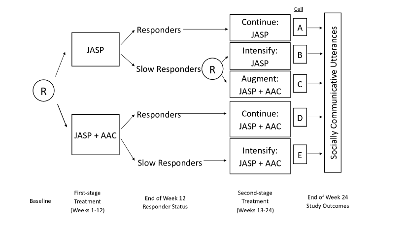
The SMART shown in Figure 1 (Kasari and others, 2014) involved children, between five and eight years old, who had a previous diagnosis of autism spectrum disorder and were considered “minimally verbal” (used fewer than 20 spontaneous different words during a baseline 20-minute language test). All eligible children were initially randomized, with equal probability, to a behavioral treatment, called JASP, or to JASP together with a speech-generating device, called AAC (augmentative or alternative communication). Both of these first-stage treatment arms in the SMART involved twice-weekly sessions with a trained language therapist. The first-stage JASP+AAC arm required that the AAC device was used at least 50 percent of the time during these sessions.
At the end of the first treatment stage, which lasted 12 weeks, all children were classified as “responders” or “slow responders”. Response was defined, prior to the trial, as an improvement of at least 25 percent on seven or more language measures (e.g. words used per minute) by the end of week 12. Children who did not satisfy this criterion were considered slow responders.
The second-stage treatments were determined as follows. Responders to the initial intervention were continued on that intervention for an additional 12 weeks. Slow responders to JASP+AAC were offered intensified JASP+AAC, which involved increasing the number of weekly sessions from two to three. Slow responders to JASP were re-randomized, with equal probability, to either intensified JASP or to JASP+AAC. The status of “responder” or “slow responder” in this SMART is known as an embedded tailoring variable, since it is used to restrict subsequent randomizations and is therefore a part of the embedded DTRs. The primary research outcome in this SMART was the total number of spontaneous socially communicative utterances in a 20-minute language sample, measured by an independent evaluator who was blind to the assigned treatment sequence. This primary outcome was measured four times: prior to the initial randomization (baseline), prior to the second randomization (at week 12), at the end of treatment (week 24) and at a follow-up assessment (week 36).
2.2 Dynamic Treatment Regimens Embedded in a SMART
A dynamic treatment regimen (DTR) is a sequence of decisions rules that, for all individuals in a population of interest, guides the provision of treatment at each decision point based on information known up to that decision point. In the case of the autism SMART, a DTR is a sequence of decision rules that guides the first and second treatment decisions for both responders and slow responders.
Specifically, the autism SMART has three DTRs embedded within it. These are listed in Table Acknowledgments. The DTR labeled (AAC, AAC+) starts with JASP and AAC, continues this treatment for responders and intensifies this treatment for slow responders. The other two DTRs start with JASP only. For slow responders, (JASP, JASP+) intensifies JASP alone while (JASP, AAC) augments JASP with AAC. Many SMARTs use a two-stage design in which only slow responders are randomized at the start of the second stage (Kidwell, 2014; Gunlicks-Stoessel and others, 2016, e.g.). In this SMART, however, second-stage randomization was restricted based on a combination of first-stage treatment and response status. We use to index the DTRs embedded in the SMART, where denotes the treatment provided at the th decision point. Table Acknowledgments enumerates the values of for each DTR in the autism SMART.
3 Linear Mixed Models for Comparing Embedded DTRs
We aim to develop a linear mixed model for primary aim comparisons based on a pre-specified summary of the mean outcome under each DTR in a SMART. To do this, we use the potential outcomes framework to describe the sequence of primary outcome measurements as a function of the embedded DTRs. For simplicity, we focus on two-stage designs. With slight changes in notation, the methodology presented here may be generalized to more complex SMART designs.
3.1 Potential outcomes and observed data
For each embedded DTR, indexed by where , and for the th SMART participant, , let denote the vector of time-ordered, potential outcome repeated measures. The vector is simply the set of longitudinal potential outcomes for participant under DTR . For example, in the case of the autism SMART, each participant has three potential values of , corresponding to the three values for given in Table Acknowledgments. Note that in the autism study, is undefined for the DTR beginning with JASP+AAC, since that DTR is fully characterized by (slow responders to JASP+AAC were not re-randomized). Let be the potential outcome for the binary embedded tailoring variable under first-stage treatment .
During the conduct of a SMART, we collect the following observed data: , the observed primary outcome for participant at time point ; , the th participant’s observed binary tailoring variable; , a pre-specified vector of baseline covariates collected prior to the first randomization; and , the random treatment assignments in the first and second stage, respectively.
In the autism SMART, the primary outcome was collected for all children at each of measurement occasions, occurring 12 weeks apart. So in this example we let denote the time, in weeks, since baseline assessment. In the autism SMART, is equal to or with equal probability, indicating randomization to either JASP or JASP+AAC. Among slow responders to JASP, that is, among all subjects with and , equals or with equal probability, denoting randomization to receive either intensified JASP or the AAC device. In the autism study, is not defined for responders and participants randomized to .
3.2 The model
For the th participant and for a fixed DTR , consider the following linear mixed effects model:
| (1) |
where is an unknown -dimensional parameter, is a -dimensional () latent random vector (the random effects) with and is the -length vector of within-subject residual errors with . We also assume that is independent of , given . The design matrix depends on the SMART design and a chosen model for the mean, conditional on the baseline covariate vector . The random effects design matrix is a function of time, , and chosen so that models subject-specific deviations from the mean over time. Since indexes the embedded DTRs and is not a random variable, and are random variables only as a function of . (In this article we do not treat as a random variable.) Note that model (1) implies that and .
With model (1), we make primary aim comparisons among embedded DTRs based on the linear, parametric marginal model for given by , where is the row of evaluated at . This is a marginal mean model in that is marginal over both the embedded tailoring variable, , and any other intermediate random variables possibly impacted by or . For the autism SMART, an example marginal mean model used previously (Lu and others, 2016; Almirall and others, 2016) is a piecewise linear model with a knot at week :
| (2) |
where is the indicator function, , , and is the mean-centered age at baseline. In this case,
In this example, the parameters , , and have a causal interpretation and can be used to specify the DTR effect estimands of primary interest. An example estimand of primary interest may be an end-of-treatment comparison between the DTR with no AAC, and the DTR with the highest dose of AAC, . Other DTR effect estimands are similarly formed via linear combinations of , , and .
In addition to specifying as a model for , model (1) implicitly defines a working model for the marginal covariance . Since we assume and are independent given , we have . Previously, models for SMARTs with a longitudinal outcome involved directly specifying a working model for (Seewald and others, 2018; Almirall and others, 2016; Lu and others, 2016). In contrast, the working model for in (1) is a consequence of separately modeling within-subject and between-subject variation via and . Together, the variance and covariance structures specified for and imply a working model for .
4 Estimation and prediction
To derive a set of estimating equations for , we initially consider the following two distributional assumptions, which are typical for a mixed model like (1):
| (3) |
With the addition of the assumptions in (3), we have with . Based on this distribution for , the log-likelihood for a sample of participants under DTR is
| (4) | ||||
In practice, this log-likelihood cannot be maximized since the potential outcomes are not observed for all participants under all DTRs in a SMART. Instead, we propose a weighted pseudo-likelihood based on the observed data collected in a SMART.
4.1 Pseudo-Likelihood Estimation
The log-likelihood (4) is a function of the following parameters: , and the unique parameters in . We let denote the vector of unique variance parameters in , including . For example, if is a scalar random variable and for all and , then . For brevity, we often suppress notation indicating that depends on . Given the observed data in a SMART, defined in section 3.1, the pseudo-likelihood we use to estimate is
| (5) |
where and . The indicator is equal to one if and only if the sequence is observable under DTR . For example, in the autism SMART, , where equals if the event occurs and equals zero otherwise. The design-specific weight is an inverse probability weight for the DTR which depends on because second-stage randomization is restricted according to this binary tailoring variable. In the autism SMART, and in many two-stage designs, only individuals with are re-randomized, and (When is not defined for a given value of , we set .)
Differentiating (5) with respect to leads to the following -dimensional set of estimating equations:
| (6) |
with the solution
| (7) | ||||
Substituting into (5), we can obtain estimates of by first computing and then estimating with . In the following theorem we derive the asymptotic properties of .
Theorem 4.1.
Define and let be the solution to given in (7). Assume the following:
-
i.
Correctly specified marginal model:
-
ii.
Sequential randomization: is independent of given ; is independent of given ; and is independent of given .
-
iii.
Consistency: and
where for all .
-
iv.
Positivity: and for any , .
-
v.
Regularity conditions: For any given , converges to some at rate, and
Then is consistent for and has an asymptotic distribution, where and
The diagonal entries of provide approximate standard errors for , where , , and
The proof of Theorem 4.1 is given in the appendix. Note that assumption (ii) and (iv), above, will be satisfied by design of the SMART, while assumption (iii) connects the observed data to the potential outcomes. Theorem 4.1 does not require the two assumptions in (3) to be true. These standard distributional assumptions were used only to motivate the pseudo-likelihood and set of estimating equations which led to an estimator for .
Given , the estimating equation (6) is identical, with slight changes in notation, to the estimating equation in Lu and others (2016) for the parameters of the marginal mean model. Estimation of in Lu and others (2016) differs from our approach primarily in its modeling and estimation procedure for . In Lu and others (2016), the form of (e.g. autoregressive) is proposed by the data analyst and an estimate of is obtained via the method of moments. In our case the form of is a result of specifying and the variance-covariance of and , while the estimate of is computed by maximizing a weighted pseudo-likelihood.
As in Lu and others (2016), Theorem 4.1 implies that is consistent for and has an asymptotic Gaussian distribution, regardless of whether converges to the true value of in model (1). This means that the random effects structure can be misspecified and the estimator will remain unbiased. However, the simulation results in Section 5 show that specifying a random effects structure which more closely models the true subject-to-subject variation in can lead to greater efficiency in estimating . Before demonstrating the performance of our estimator in simulation studies, we propose a method for predicting the value of in model (1) and hence predicting subject-specific trajectories for the primary outcome in a SMART.
4.2 Random Effects Prediction
The estimator for derived above is all that is necessary for primary aim comparisons among the DTRs embedded in a SMART. Recall that a secondary motivation for using linear mixed models is the prediction of subject-specific outcome trajectories under specific DTRs. In this section we propose a method of predicting in (1) using the weighted pseudo-likelihood in (5).
In Theorem 4.1 we do not require knowledge of or the distributions of and . To predict , however, we assume that the distributional assumptions in (3) are true in the population of potential outcomes. Specifically, under model (1), assuming (3), has a multivariate Gaussian distribution, which implies that
| (8) |
where . If all potential outcomes were observed for each participant, a plug-in estimator of based on (8) would serve as a prediction of . Instead, motivated by (8), we propose the following:
| (9) | ||||
| (10) | ||||
In practice, the predictions for each participant are obtained by substituting the estimates and into (10), so that . (Recall that estimates for the entries of are given by some of the components of .) This predictor can be regarded as an empirical Bayes predictor for (Skrondal and Rabe-Hesketh, 2009; Carlin and Louis, 2000) with weights that adjust for the probability of observing responders and slow responders under each embedded DTR.
5 Simulations studies
Next we use simulation studies to evaluate the ability of our mixed effects model to estimate causal estimands of primary interest when comparing embedded DTRs in a SMART. We also compare our mixed model estimator to the GEE-like estimators discussed in Lu and others (2016) and Seewald and others (2018).
Data were generated from a hypothetical SMART with two treatment stages, two treatment options for all participants in stage one, and two treatment options for slow responders in stage two, leading to four embedded DTRs with . This is a common SMART design (Naar-King and others, 2016; August and others, 2016, e.g.) and is different from the autism SMART in Figure 1, in which slow responders from only one of the stage-one treatment arms were randomized at the start of the second stage. In a given simulation replicate, potential outcomes were generated according to (24), below, and observed data were obtained from these potential outcomes via randomizations satisfying assumptions (ii) and (iii) in Theorem 4.1. All simulated participants were randomized with equal probability to either or , and only slow responders were randomized to or with equal probability.
The potential outcomes in these simulation studies were generated from the following piecewise linear model:
| (11) | ||||
where ; ; and with . The binary tailoring variable is a function of the potential outcome at the end of the first treatment stage, and the fixed value of means that varies as a function of . The parameters and induce a marginal association between and second-stage outcomes. The random intercepts and slopes, and , induce within-person correlation, and the residual errors were generated independently across and . The scalar random variable is a binary baseline covariate, and the knot represents the time when the first treatment stage ends. In all simulations, half of the participants were assigned and half were assigned . Under (24), the marginal mean can be expressed as follows:
| (12) | ||||
and causal estimands of primary interest are expressed as functions of , and . Further details of this generative model are given in the appendix.
Below we present the results of two simulation studies which differ in whether or not they misspecify the marginal variance and distribution of . In both cases, the linear model for is correctly specified. We report estimation performance for the end-of-study contrast and we chose simulation parameters so that this contrast had the largest magnitude among any pairwise contrast between embedded DTRs. Parameter values for the marginal mean were chosen to achieve desired values of the standardized effect size .
5.1 Simulation 1
The first simulation study verifies that our estimator is unbiased in large samples and that large-sample confidence interval coverage is attained with the standard errors based on Theorem 4.1. This is accomplished in the ideal setting in which the probability distribution of can be correctly specified using our proposed mixed model. In general, in (24) follows a Gaussian mixture distribution with mixing probability . However, in this simulation study we choose , so that and the distribution of is the same as the marginal distribution specified in the following mixed model:
| (13) |
where is the linear parametrization of the mean in equation (12). We compared this “slopes and intercepts” mixed model, in which the joint distribution of is correctly specified, to an “intercepts only” mixed model,
| (14) |
in which is misspecified. We use different notation for the random effects and variance parameters in (13)–(14) than we do in (24) to distinguish models used for estimation from the true, data-generating probability distribution. In this simulation study we set and .
Table Acknowledgments contains the bias and standard deviation of the point estimates, the mean of the approximate standard errors, the coverage probability for a 95-percent confidence interval, and the root mean squared error (RMSE) computed from 1,000 simulation replicates. In large samples, the bias is approximately two orders of magnitude smaller than the standard deviation of the point estimates, confirming that the mixed model estimator is unbiased for the linear mean parameters in (12). The standard errors based on Theorem 4.1 provide confidence interval coverage close to the nominal level in large samples. In addition, note that the intercepts only mixed model, which misspecifies , does not introduce bias in large samples. Instead, the estimator is slightly less efficient than the slopes and intercepts model, in which both the mean and covariance of are correctly specified.
5.2 Simulation 2
In this second simulation, we investigate whether the estimator is unbiased in large samples, and whether this estimator can provide efficiency gains relative to existing estimators, in a more realistic scenario in which it is not possible to correctly specify the distribution of using model (1). Data were again generated from model (24), but the coefficients and were nonzero and therefore had a marginal Gaussian mixture distribution.
In addition to the mixed models (13)–(14), we also report estimation performance of the GEE-like estimator of Lu and others (2016) and Seewald and others (2018). With these GEE estimators, a working model for (e.g. exchangeable) is specified directly and the method of moments is used to estimate the parameters in this working model. A complete description of our implementation of these GEE estimators is given in the appendix. In this simulation study, all of the models used for estimation correctly specify the linear model , but none of them correctly specify the marginal covariance or the distribution of .
Table Acknowledgments compares the two mixed models and the GEE estimator with exchangeable, unstructured, and independence working models for in their ability to estimate the end-of-study contrast with standardized effect size . The magnitude of the bias relative to the standard deviation in Table Acknowledgments indicates that all of these estimators are unbiased in large samples.
While none of the estimation models in this simulation study correctly specify , we can see in Table Acknowledgments that efficiency (measured by RMSE) is improved by a working model which more closely resembles the true marginal covariance. Here we report RMSE as a fraction of the smallest RMSE for a fixed sample size. To measure the performance of each working model for , we report , the relative error in the Frobenius norm between , the true average covariance matrix of according to the generative model, and the simulation-based estimate of , the large-sample average covariance matrix implied by the estimation model. The slopes and intercepts mixed model had both the lowest relative error in estimating and the lowest RMSE for each fixed sample size. For these estimators, RMSE decreases as the working model for improves. This simulation study suggests that if the separate specification of between-person and within-person variation in a mixed effects model leads to improved modeling of the marginal covariance, we can expect efficiency gains over GEE-like approaches when comparing embedded DTRs.
6 Application
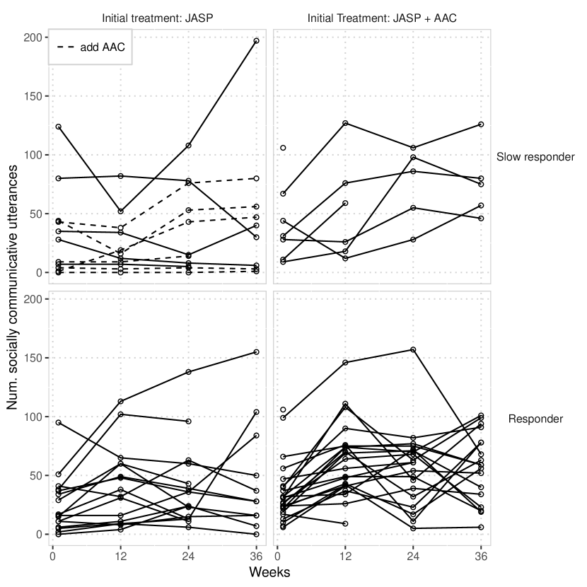
Finally, we demonstrate our mixed model using the autism SMART of Kasari and others (2014). Our goal here is to compare the three embedded DTRs based on changes in communication outcomes for the children receiving each DTR. Figure 2 displays the measured primary outcome, the number of socially communicative utterances, for each participant in this study at baseline and at weeks 12, 24, and 36. For the marginal mean, we specified the piecewise linear model (2), and we specified random intercepts as the random effects structure.
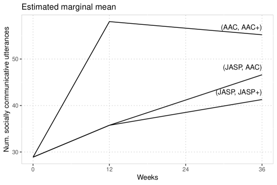
The parameter vector was estimated as described in Section 4.1 using widely available software for linear mixed models (Bates and others, 2015) applied to a restructured version of the observed data. This software implementation is described in greater detail in the appendix. The estimates of and obtained in this manner were then used to compute estimated standard errors as described in Section 4.1. Table Acknowledgments displays the estimated coefficients in this model with 95-percent confidence intervals, and Figure 3 displays the estimated marginal mean for each DTR at each time point,
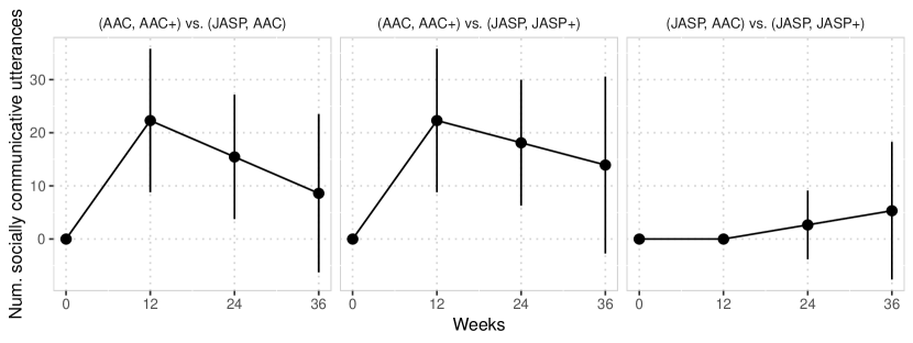
To understand whether we have evidence that communication outcomes differ among children receiving each of these DTRs, we performed an “omnibus” test of whether the three DTRs differ at all. We tested the hypothesis that the area under the curve (AUC) for the marginal mean is the same across all three DTRs, which, in this case, is equivalent to testing for a constant matrix . Based on Theorem 4.1, under , the statistic , where is the estimated covariance matrix of , has a distribution with two degrees of freedom in large samples. This test statistic was equal to with a -value of , suggesting differences in the AUCs among the three DTRs. Following this omnibus test, we examined pairwise contrasts between each DTR at each time point, given in Figure 4, which suggest that the DTR which starts with the AAC speech device is superior to the other two DTRs, at least during the first 12 weeks.
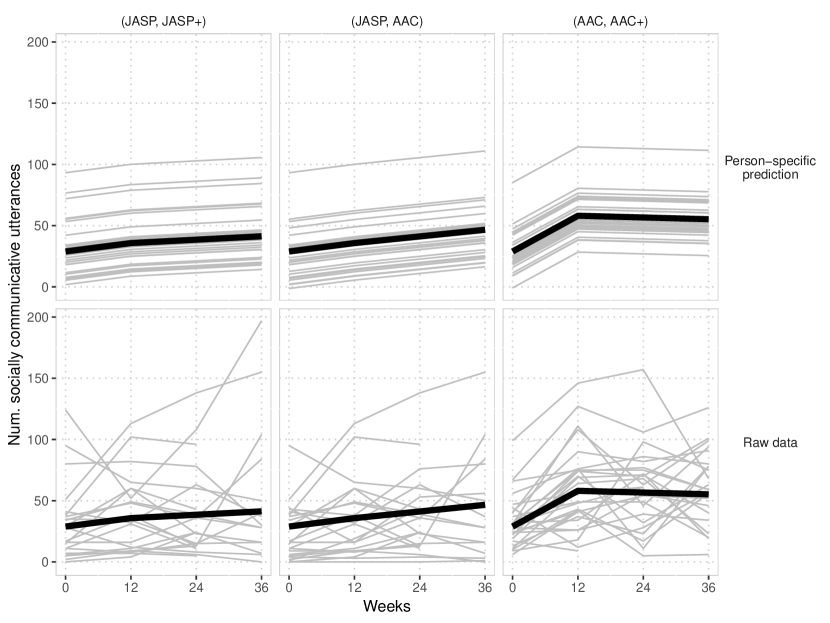
For demonstration, Figure 5 displays predicted person-specific trajectories, , using the intercepts-only mixed model, along with the observed outcomes and the estimated mean outcome under each DTR. This display could be used to assess subject-to-subject variation relative to the estimated mean under each DTR or to identify individuals with outlying trajectories based on the fitted model. In this example, random intercepts lead to subject-specific trajectories which are parallel to the estimated mean under each DTR. The potential high outliers under the DTRs (JASP, AAC) and (AAC, AAC+) could be investigated to help characterize the variation in communication outcomes for these study participants.
7 Discussion
In Section 4.2 we proposed a method for predicting random effects based on a weighted pseudo-likelihood. The prediction method we propose is analogous to the “best linear unbiased predictors” commonly used in standard mixed effects analysis of longitudinal data (Robinson, 1991; Verbeke and Molenberghs, 2009, Section 7.4). However, our proposed predictor is a nonlinear function of across all , and it is unclear whether has minimum mean squared error (MSE) marginally over these random variables. Further work is needed to derive a minimum-MSE property for which is marginal over and uses the same statistical and causal assumptions of Theorem 4.1.
This article focused on marginal mean models for the embedded DTRs that are conditional only on baseline covariates. This is analogous to primary aim analyses in standard randomized trials. An alternative approach would be to specify a mixed model conditional on both the baseline covariates and the embedded tailoring variables. For example, in the autism SMART, one could propose a mixed effects model for conditional on . Future work will investigate how to obtain consistent estimators for marginal estimands using this kind of conditional modeling of the observed longitudinal outcome.
In addition to the reasons given in Section 1, scientists might prefer mixed effects models because they may require less restrictive assumptions about missing data, at least when the true probability distribution for the observed data is correctly specified (Hedeker and Gibbons, 2006, Ch. 14; Fitzmaurice and others, 2012, Ch. 17) Our marginal modeling and weighted, pseudo-likelihood estimation approach does not require a correct specification of the true probability distribution that generated the observed data. Additional work is needed to understand whether our marginal model for longitudinal SMARTs enjoys the purported benefits of standard mixed models in the presence of missing data. In the appendix we present simulation results which suggest that our mixed model may offer some protection against bias in the presence of ignorable missing data.
Acknowledgments
This research is supported by the following NIH grants: R01DA039901 (Nahum-Shani and Almirall), P50DA039838 (Almirall), R01HD073975 (Kasari and Almirall), R01MH114203 (Almirall), and R01DA047279 (Almirall).
Conflict of Interest: None declared.
The dynamic treatment regimens embedded in the example autism SMART. The last column provides the known inverse probability weight for subjects in each of the cells A–E in Figure 1. First-stage Status at end Second-stage Cell in Known DTR Label Treatment of first-stage Treatment Figure IPW (JASP, JASP+) JASP Responder Continue JASP A 2 Slow Responder Intensify JASP B 4 (JASP, AAC) JASP Responder Continue JASP A 2 Slow Responder Augment JASP+AAC C 4 (AAC, AAC+) JASP+AAC Responder Continue JASP+AAC D 2 Slow Responder Intensify JASP+AAC E 2
Estimation performance of an end-of-study contrast with two mixed model specifications when the population of potential outcomes exactly follows the marginal distribution implied by the slopes and intercepts mixed model. The intercepts only model specifies the correct mean model but is otherwise misspecified. Values compuuted from 1,000 simulation replicates. The nominal confidence level was 95 percent. Method True value N Bias Monte Carlo SD SE Estimate CI Coverage RMSE LMM slopes and intercepts 0.2 0.600 50 -0.102 1.222 1.119 0.911 1.226 200 -0.018 0.659 0.629 0.931 0.659 1000 0.010 0.296 0.290 0.945 0.296 5000 -0.002 0.132 0.130 0.945 0.132 0.8 2.480 50 0.071 1.228 1.117 0.905 1.229 200 -0.002 0.661 0.623 0.932 0.661 1000 -0.008 0.285 0.286 0.950 0.285 5000 -0.007 0.129 0.128 0.948 0.129 LMM intercepts only 0.2 0.600 50 -0.018 1.338 1.196 0.886 1.338 200 0.001 0.748 0.694 0.917 0.748 1000 0.010 0.336 0.323 0.938 0.336 5000 0.002 0.146 0.145 0.951 0.146 0.8 2.480 50 0.148 1.339 1.191 0.888 1.346 200 0.011 0.728 0.682 0.922 0.727 1000 -0.006 0.312 0.317 0.957 0.311 5000 -0.005 0.143 0.142 0.957 0.143
Simulation 2: Estimation of an end-of-study contrast with true value and standardized effect size . Values computed from 1,000 simulation replicates. The nominal confidence level was 95 percent. RMSE inflation is the ratio of the RMSE to the smallest RMSE among the five methods for a fixed sample size. N Method Bias Monte Carlo SD SE Estimate CI Coverage RMSE Inflation 50 LMM slopes and intercepts 0.013 1.655 1.505 0.910 1.000 0.051 GEE Unstructured 0.064 1.761 1.452 0.854 1.064 0.107 LMM intercepts only 0.115 1.922 1.656 0.871 1.163 0.640 GEE Exchangeable 0.114 1.924 1.651 0.870 1.164 0.643 GEE Independence 0.182 2.163 1.804 0.861 1.311 0.900 200 LMM slopes and intercepts -0.041 0.842 0.839 0.938 1.000 0.015 GEE Unstructured -0.019 0.878 0.822 0.925 1.042 0.028 LMM intercepts only 0.002 0.983 0.951 0.930 1.167 0.638 GEE Exchangeable 0.002 0.984 0.950 0.931 1.167 0.638 GEE Independence 0.016 1.099 1.055 0.936 1.305 0.900 1000 LMM slopes and intercepts -0.006 0.396 0.385 0.948 1.000 0.009 GEE Unstructured -0.003 0.410 0.384 0.933 1.034 0.011 LMM intercepts only 0.011 0.442 0.439 0.950 1.115 0.637 GEE Exchangeable 0.011 0.442 0.439 0.949 1.115 0.637 GEE Independence 0.021 0.483 0.489 0.950 1.220 0.900 5000 LMM slopes and intercepts 0.000 0.172 0.174 0.958 1.000 0.007 GEE Unstructured -0.001 0.178 0.174 0.947 1.039 0.007 LMM intercepts only 0.005 0.204 0.198 0.936 1.191 0.637 GEE Exchangeable 0.005 0.204 0.198 0.936 1.191 0.637 GEE Independence 0.005 0.227 0.221 0.947 1.323 0.900
Coefficient estimates, standard errors (SE) and 95-percent confidence intervals from the random intercepts mixed model for the autism SMART. Coefficient Estimate SE 95% CI 28.885 3.763 1.501 0.315 0.287 0.112 0.174 0.23 0.174 0.137 2.777
This appendix contains the following: a proof of Theorem 4.1; further description of the GEE estimator used as a comparison method in the simulation studies in Section 5; results of a simulation study with ignorable missing data; and a description of how the weighted pseudo-likelihood was implemented with standard mixed models software for the analysis in Section 6.
Appendix A Proof of Theorem 4.1
First note that , , and . To simplify notation, we suppress dependence of and on . Then, by definition of ,
| (15) | ||||
and, using consistency assumption (ii)
| (16) | ||||
Next note that and, by assumption (iii), for any fixed regime . Let .
| (17) | |||
| (18) | |||
| (19) | |||
| (20) |
Substituting into equation (16),
| (21) | ||||
| (22) | ||||
| (23) | ||||
where (22) is obtained from the consistency assumption on and independence of and . Thus . Under Assumption (v), we have that is a consistent estimator of . To derive the asymptotic distribution of , note that
The result follows using similar arguments as those in the proof of Theorem 2 in Liang and Zeger (1986).
Appendix B Details of the GEE estimator used in simulation
Here we describe the GEE-like estimator of Lu and others (2016) and Seewald and others (2018) used as a comparison method in the simulations in Section 5.
First, an initial least squares estimate is computed:
This initial estimate is used to compute the residual vectors for all and .
Next we compute method of moments estimators for . Let be the number of embedded DTRs, i.e. . For , define the following:
where is the number of individuals with an observation at unique time point and is the number of individuals with observations at both of the time points and . The estimators defined above are simply the method of moments estimators for correlation or variance parameters at each observation. They differ in whether the variances or correlations are assumed to be equal across DTRs and in whether the variance is assumed to be constant as a function of time. By combining these correlation and variance estimators, we can obtain various working models for . For example, the unstructured and exchangeable estimates of have the following entries, :
| Unstructured | Exchangeable | ||||
The independence working model sets all off-diagonal entries of to zero and all diagonal entries to .
Autoregressive working models for are also possible using the following correlation estimators:
Appendix C Details of the generative model used in simulation
This section provides more detail about the generative model used in the simulation studies in Section 5.
The potential outcomes were generated from the following piecewise linear model:
| (24) | ||||
where ; ; ; ; with ; ; and .
Under model (24),
| (25) | ||||
and we can parameterize this marginal mean model as follows:
| (26) | ||||
where for and
Next, we derive the marginal covariance and variance of the repeated measures outcomes under this generative model. These marginal covariances and variances are used to calculate the population standardized effect size
Let and . Then
| (27) | ||||
where
Note that
and since is bivariate Gaussian, can be computed using the truncated multivariate Gaussian distribution.
Appendix D Additional simulation study
One potential benefit of mixed models is their ability to provide unbiased parameter estimates when data are missing at random, assuming that estimation and inference are based on a correctly specified likelihood for the observed data (Fitzmaurice and others, 2012, Ch. 17; Hedeker and Gibbons, 2006, Ch. 14; Molenberghs and Kenward, 2007, Ch. 7; Gibbons and others, 2010). In the case of the mixed model we propose for longitudinal SMARTs, estimation and inference are based on a weighted pseudo-likelihood, not the true likelihood for the observed data, so it is not clear whether bias can be avoided with ignorable missing data in a SMART.
To help understand whether mixed models provide any protection against bias due to missing data in a longitudinal SMART, this additional simulation study describes the performance of our mixed model and the GEE-like estimators of Seewald and others (2018) and Lu and others (2016) when data are missing at random (ignorable) due to study dropout. In this scenario, if a participant’s observed at was less than , then all observations from that participant at time points were discarded. This results in about 20 percent dropout among participants with ; about 17 percent dropout among participants with ; about nine and ten percent dropout among participants with and , respectively; and less than percent dropout among participants with .
Table E compares the same estimators from Simulation 2 in the Section 5 in their ability to estimate an end-of-study contrast with effect size in the presence of the dropout process described above. In this scenario, we see bias in large samples, although the degree of bias decreases as decreases. This suggests that the ability of a mixed model to flexibly model , and to efficiently estimate , may provide some protection against bias due to ignorable missing data. Since we are not able to fit a mixed model using the true likelihood for the potential outcomes, the purported benefits of mixed models in the presence of ignorable missing data (compared to GEE approaches) might not exist when analyzing longitudinal SMARTs.
Appendix E Software implementation with integer-valued weights
Next we describe how the mixed model for longitudinal SMARTs can be implemented using standard mixed model software, such as Bates and others (2015). This implementation is limited to analyses in which the weights are integer-valued. When estimating these probability of treatment weights (Hirano and others, 2003; Brumback, 2009) or when randomization probabilities are unequal across treatment options, the weights may not be integer-valued. Future work will develop software implementations for use in SMART designs beyond the special case of integer-valued weights.
Recall that is an indicator of whether subject is observable under regimen . For example, in the autism study, . Let be an arbitrary function of the observed response vector , baseline covariates , and the DTR . In the autism SMART and other common designs, responders () are observable under both of the DTRs . In this case,
| (28) | ||||
since when , subject is observable under DTR only.
The weighted pseudo-likelihood is
| (29) | ||||
| (30) | ||||
This objective function is equivalent to the log-likelihood in a linear mixed effects model based on an “augmented” data set constructed in the following manner. For all subjects whose observed data are observable under more than one DTR, duplicate the baseline covariates and response vectors once for each of those DTRs. In the autism SMART, subjects with are observable under and , so the baseline covariates and response vectors are duplicated twice. The design matrices and for each replicate are formed by plugging in the values of corresponding to the DTR under which that replicate is observable. The weights for these replicates are formed similarly. Thus, for a subject with , the augmented data consist of
For subjects whose observed data are observable only under the DTR , their observed data are unchanged and included in the augmented data set.
Indexing the artificial “subjects” in the augmented data set by , we have, based on (30),
| (31) |
where and are the values of , and evaluated under the DTR corresponding to replicate in the augmented data. Thus, to find maximum likelihood estimates of the parameters and , we can use any software package which maximizes a weighted log-likelihood of the form (31). In particular, when is an integer, we can maximize (31) by duplicating all of the terms indexed by a total of times and fitting the mixed model corresponding to (31) without the use of weights.
Simulation 3: Estimation performance with ignorable missing data due to study dropout. The true contrast value is , corresponding to a standardized effect size of . Values computed from 1,000 simulation replicates. The nominal confidence level was 95 percent. N Method Bias Monte Carlo SD SE Estimate CI Coverage RMSE Inflation 200 LMM slopes and intercepts -0.066 0.887 0.836 0.929 1.000 0.046 GEE Unstructured -0.127 0.900 0.789 0.906 1.023 0.257 LMM intercepts only -0.401 0.950 0.891 0.900 1.161 0.660 GEE Exchangeable -0.402 0.951 0.890 0.900 1.161 0.663 GEE Independence -0.559 1.047 0.983 0.881 1.335 0.904 1000 LMM slopes and intercepts -0.103 0.389 0.381 0.939 1.000 0.044 GEE Unstructured -0.158 0.396 0.366 0.902 1.059 0.246 LMM intercepts only -0.445 0.419 0.408 0.796 1.519 0.659 GEE Exchangeable -0.445 0.419 0.408 0.795 1.519 0.661 GEE Independence -0.612 0.464 0.451 0.699 1.907 0.904 5000 LMM slopes and intercepts -0.080 0.177 0.171 0.921 1.000 0.042 GEE Unstructured -0.138 0.178 0.165 0.848 1.157 0.243 LMM intercepts only -0.437 0.187 0.184 0.349 2.448 0.658 GEE Exchangeable -0.437 0.187 0.184 0.350 2.448 0.660 GEE Independence -0.614 0.204 0.203 0.134 3.332 0.904
References
- Almirall and others (2016) Almirall, D., DiStefano, C., Chang, Y., Shire, S., Kaiser, A., Lu, X., Nahum-Shani, I., Landa, R., Mathy, P. and Kasari, C. (2016). Longitudinal effects of adaptive interventions with a speech-generating device in minimally verbal children with ASD. Journal of Clinical Child and Adolescent Psychology 45, 442–456.
- Almirall and others (2014) Almirall, D., Nahum-Shani, I., Sherwood, N. and Murphy, S. A. (2014). Introduction to SMART designs for the development of adaptive interventions: with application to weight loss research. Translational Behavioral Medicine 4, 260–274.
- August and others (2016) August, G. J., Piehler, T. F. and Bloomquist, M. L. (2016). Being “SMART” about adolescent conduct problems prevention: executing a SMART pilot study in a juvenile diversion agency. Journal of Clinical Child and Adolescent Psychology 45, 495–509.
- Bates and others (2015) Bates, D., Mächler, M., Bolker, B. and Walker, S. (2015). Fitting linear mixed-effects models using lme4. Journal of Statistical Software 67, 1–48.
- Brumback (2009) Brumback, B. A. (2009). A note on using the estimated versus the known propensity score to estimate the average treatment effect. Statistics and Probability Letters 79, 537–542.
- Carlin and Louis (2000) Carlin, B. P. and Louis, T. A. (2000). Empirical Bayes: Past, present and future. Journal of the American Statistical Association 95, 1286–1289.
- Chakraborty and Moodie (2013) Chakraborty, B. and Moodie, E. E. (2013). Statistical methods for dynamic treatment regimes. Springer.
- Dawson and Lavori (2008) Dawson, R. and Lavori, P. W. (2008). Sequential causal inference: Application to randomized trials of adaptive treatment strategies. Statistics in medicine 27, 1626–1645.
- Diggle and others (2002) Diggle, P., Heagerty, P., Liang, K. and Zeger, S. (2002). Analysis of longitudinal data. Oxford University Press.
- Dziak and others (2019) Dziak, J. J., Yap, J. R. T., Almirall, D., McKay, J. R., Lynch, K. G. and Nahum-Shani, I. (2019). A data analysis method for using longitudinal binary outcome data from a smart to compare adaptive interventions. Multivariate Behavioral Research 54, 613–636.
- Fitzmaurice and others (2012) Fitzmaurice, G. M., Laird, N. M. and Ware, J. H. (2012). Applied longitudinal analysis, Volume 998. John Wiley and Sons.
- Gibbons and others (2010) Gibbons, R. D., Hedeker, D. and DuToit, D. (2010). Advances in analysis of longitudinal data. Annual review of clinical psychology 6, 79–107.
- Goldstein (2011) Goldstein, H. (2011). Multilevel statistical models, Volume 922. John Wiley and Sons.
- Gunlicks-Stoessel and others (2016) Gunlicks-Stoessel, M., Mufson, L., Westervelt, A., Almirall, D. and Murphy, S. A. (2016). A pilot SMART for developing an adaptive treatment strategy for adolescent depression. Journal of Clinical Child and Adolescent Psychology 45, 480–494.
- Hedeker and Gibbons (2006) Hedeker, D. and Gibbons, R. D. (2006). Longitudinal data analysis, Volume 451. John Wiley and Sons.
- Hernán and others (2006) Hernán, M.A., Lanoy, E., Costagliola, D. and Robins, J. M. (2006). Comparison of dynamic treatment regimes via inverse probability weighting. Basic and Clinical Pharmacology and Toxicology 98, 237–242.
- Hirano and others (2003) Hirano, K., Imbens, G. W. and Ridder, G. (2003). Efficient estimation of average treatment effects using the estimated propensity score. Econometrica 71, 1161–1189.
- Kasari and others (2014) Kasari, C., Kaiser, A., Goods, K., Nietfeld, J., Mathy, P., Landa, R., Murphy, S. A. and Almirall, D. (2014). Communication interventions for minimally verbal children with autism: a sequential multiple assignment randomized trial. Journal of the American Academy of Child and Adolescent Psychiatry 53, 635–646.
- Kidwell (2014) Kidwell, K. M. (2014). SMART designs in cancer research: past, present, and future. Clinical Trials 11, 445–456.
- Kosorok and Moodie (2015) Kosorok, M. R. and Moodie, E. E. M. (2015). Adaptive treatment strategies in practice: planning trials and analyzing data for personalized medicine, Volume 21. SIAM.
- Lavori and Dawson (2000) Lavori, P. and Dawson, D.A. (2000). A design for testing clinical strategies: biased individually tailored within-subject randomization. Journal of the Royal Statistical Society, Series A 163, 29–38.
- Lavori and Dawson (2014) Lavori, P. W. and Dawson, R. (2014). Introduction to dynamic treatment strategies and sequential multiple assignment randomization. Clinical Trials 11, 393–399.
- Lei and others (2012) Lei, H., Nahum-Shani, I., Lynch, K., Oslin, D. and Murphy, S. A. (2012). A SMART design for building individualized treatment sequences. Annual Review of Clinical Psychology 8, 21–48.
- Li and Murphy (2011) Li, Z. and Murphy, S. A. (2011). Sample size formulae for two-stage randomized trials with survival outcomes. Biometrika 98, 503–518.
- Liang and Zeger (1986) Liang, K. and Zeger, S. L. (1986). Longitudinal data analysis using generalized linear models. Biometrika 73, 13–22.
- Lu and others (2016) Lu, X., Nahum-Shani, I., Kasari, C., Lynch, K. G., Oslin, D. W., Pelham, W. E., Fabiano, G. and Almirall, D. (2016). Comparing dynamic treatment regimes using repeated-measures outcomes: modeling considerations in SMART studies. Statistics in Medicine 35, 1595–1615.
- Molenberghs and Kenward (2007) Molenberghs, G. and Kenward, M. (2007). Missing data in clinical studies, Volume 61. John Wiley and Sons.
- Murphy (2005) Murphy, S. A. (2005). An experimental design for the development of adaptive treatment strategies. Statistics in Medicine 24, 1455–1481.
- Murphy and others (2007) Murphy, S. A., Lynch, K. G., Oslin, D. W., McKay, J.R. and Tenhave, T. R. (2007). Developing adaptive treatment strategies in substance abuse research. Drug and Alcohol Dependence 88, S24–S30.
- Murphy and others (2001) Murphy, S. A., van der Laan, M. J., Robins, J. M. and Conduct Problems Prevention Research Group. (2001). Marginal mean models for dynamic regimes. Journal of the American Statistical Association 96, 1410–1423.
- Naar-King and others (2016) Naar-King, S., Ellis, D. A., Idalski Carcone, A., Templin, T., Jacques-Tiura, A. J., Brogan Hartlieb, K., Cunningham, P. and Jen, K-L. C. (2016). Sequential multiple assignment randomized trial (SMART) to construct weight loss interventions for African American adolescents. Journal of Clinical Child and Adolescent Psychology 45, 428–441.
- Nahum-Shani and others (2012) Nahum-Shani, I., Qian, M., Almirall, D., Pelham, W.E., Gnagy, B., Fabiano, G., Waxmonsky, J., Yu, J. and Murphy, S. A. (2012). Experimental design and primary data analysis methods for comparing adaptive interventions. Psychological Methods 17, 457–477.
- NeCamp and others (2017) NeCamp, T., Kilbourne, A. and Almirall, D. (2017). Comparing cluster-level dynamic treatment regimens using sequential, multiple assignment, randomized trials: regression estimation and sample size considerations. Statistical methods in medical research 26, 1572–1589.
- Orellana and others (2010) Orellana, L., Rotnitzky, A. and Robins, J. M. (2010). Dynamic regime marginal structural mean models for estimating optimal dynamic treatment regimes, Part I: main content. International Journal of Biostatistics 6, Article 8.
- Raudenbush and Bryk (2002) Raudenbush, S. W. and Bryk, A. S. (2002). Hierarchical linear models: applications and data analysis methods, Volume 1. Sage.
- Robinson (1991) Robinson, G. K. (1991). That BLUP is a good thing: The estimation of random effects. Statistical Science 6, 15–32.
- Searle and others (2006) Searle, S. R., Casella, G. and McCulloch, C. E. (2006). Variance Components. Wiley.
- Seewald and others (2018) Seewald, N. J., Kidwell, K. M., Nahum-Shani, I., Wu, T., McKay, J. R. and Almirall, D. (2018). Sample size considerations for comparing dynamic treatment regimens in a sequential multiple-assignment randomized trial with a continuous longitudinal outcome. arXiv e-prints, arXiv:1810.13094.
- Skrondal and Rabe-Hesketh (2009) Skrondal, A. and Rabe-Hesketh, S. (2009). Prediction in multilevel generalized linear models. Journal of the Royal Statistical Society—Series A 172, 659–687.
- Snijders and Bosker (2012) Snijders, T. A. B. and Bosker, R. J. (2012). Multilevel analysis: an introduction to basic and advanced multilevel modeling. Sage.
- Verbeke and Molenberghs (2009) Verbeke, G. and Molenberghs, G. (2009). Linear mixed models for longitudinal data. Springer Science and Business Media.