Automatic Generation of Multi-precision Multi-arithmetic CNN Accelerators for FPGAs

Abstract

Modern deep Convolutional Neural Networks (CNNs) are computationally demanding, yet real applications often require high throughput and low latency. To help tackle these problems, we propose Tomato, a framework designed to automate the process of generating efficient CNN accelerators. The generated design is pipelined and each convolution layer uses different arithmetics at various precisions. Using Tomato, we showcase state-of-the-art multi-precision multi-arithmetic networks, including MobileNet-V1, running on FPGAs. To our knowledge, this is the first multi-precision multi-arithmetic auto-generation framework for CNNs. In software, Tomato fine-tunes pretrained networks to use a mixture of short powers-of-2 and fixed-point weights with a minimal loss in classification accuracy. The fine-tuned parameters are combined with the templated hardware designs to automatically produce efficient inference circuits in FPGAs. We demonstrate how our approach significantly reduces model sizes and computation complexities, and permits us to pack a complete ImageNet network onto a single FPGA without accessing off-chip memories for the first time. Furthermore, we show how Tomato  produces implementations of networks with various sizes running on single or multiple FPGAs. To the best of our knowledge, our automatically generated accelerators outperform closest FPGA-based competitors by at least $2$-$4\times$ for lantency and throughput; the generated accelerator runs ImageNet classification at a rate of more than 3000 frames per second.

I Introduction

Large-scale Convolution Neural Networks (CNNs) have delivered revolutionary performance gains to vision applications such as image classification [18], object detection [21], and emotion recognition [22]. To support such workloads, both edge and cloud environments already employ the parallelism offered by GPUs and have more recently sought to optimize latency, throughput and energy with the use of FPGAs [7, 23, 34, 25, 31, 41, 2, 32, 35] and ASICs [28, 36].

As CNN models are inherently redundant, model compression is popular in making CNN inference more efficient. Methods such as low precision quantization [45, 43] and channel-wise structural pruning [10, 8] directly shrink the compute and memory requirements. These techniques have become essential for state-of-the-art CNN accelerators, as they directly translate to high throughput and low latency [9]. Unlike previous attempts [28] that unify all layers in a single arithmetic at a unified precision, we propose hybrid quantization that allows a mixture of arithmetics and precisions to minimize the effect of quantization on CNNs task accuracies. Each layer of the CNN can have different arithmetics at different precisions. In software, we implement hybrid quantization in Tomato and automate the selection of arithmetics and precisions for different layers of the CNN. Tomato then retrains the selected quantized model.

Hardware that uses a homogenous large systolic array currently dominates the design of CNN accelerators; a great number of parallel multiplication-adds are used as a large compute core and both weights and activations are buffered in on-chip memory [41, 4] (left of Figure 1). The large systolic array is time-shared as a number of different convolutions reuse the same hardware, however, various input data sizes, channel counts, kernel sizes and ever-emerging new convolutions [40] make the design of a single efficient compute core increasingly difficult. Alternatively, the computation of a CNN can also be divided and pipelined into a number of smaller compute cores (so-called Flattened Streaming). Each computation core, streamed by activations, is only responsible for the calculations of individual layers [7, 39] (right of Figure 1) to maximize efficiency. In this paper, we approach the CNN acceleration problem by exploiting the reconfigurability of FPGAs in the flattened streaming design. Tomato directly produces small layer-wise compute cores, maximizing the available logic of FPGAs for each target network. We further make the observation that flattened streaming accelerators isolate layer-wise computations, offering the chance to use different arithmetics and precisions for each layer’s computation. In addition, the throughputs can be matched across various compute cores in the flattened streaming architecture – the compute throughput of a particular layer only needs to match its preceding layer’s output generation rate. Forcing the layers to match throughputs further reduces the logic size of the auto-generated hardware.

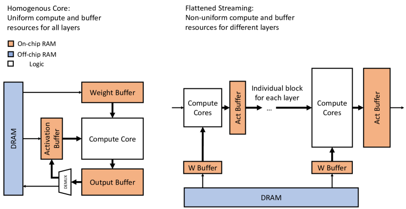
Figure 1: An illustration of a homogenous core (left) and flattened streaming cores (right).

The combination of hybrid quantization, a streaming-based architecture and ever larger FPGAs, enable us to map all the layers of our CNN onto a single or even multiple FPGAs. In this paper, we present an automated software-hardware co-design workflow that produces multi-arithmetic multi-precision CNN accelerators. The resulting hardware accelerator is streaming-based and fully pipelined. We make the following contributions in this paper:

• We demonstrate the effectiveness of hybrid quantization on modern efficient CNNs (like MobileNet-V1).

• We present a novel streaming architecture for CNNs that is pipelined and uses minimal intra-layer buffering. Each layer’s compute is matched on throughputs and is isolated and applied with various quatnizations.

• We show a full-stack automated workflow. The workflow packs entire networks into FPGAs. To the best of our knowledge, the resulting design outperforms all state-of-the-art FPGA-based CNN accelerators in terms of latency and throughput.

II Related Work

Traditional CNNs running on GPUs typically use single-precision floating-point arithmetic, which is infeasible for FPGAs with limited logic resources. Yet CNNs are, in general, often over-provisioned and inherently redundant; this makes low-precision quantization an essential technique to drastically reduce the memory consumed by the network’s parameters, and even allows CNN inference to be computed entirely with low-cost arithmetic operations, rather than floating-point ones. Many works [5, 13] train CNNs to use low-precision weights and activations with minimal accuracy loss, while others pushed the limit by using ternarized weights $\{0,\pm 1\}$ [14, 19, 46], and even constraining both weights and activations to binary values $\{\pm 1\}$ [12, 26]. However, binarized and ternarized CNNs struggle to achieve state-of-the-art accuracies on large datasets. FPGA-based accelerators generally uniformly apply one of the above quantization methods This specialisation provides efficiency and performance gains when compared to GPUs with fixed set of data types. Bit-serial accelerators [29, 30] are also of interest as they provide scope to optimise away superfluous computation at the bit-level when computing with fixed-point numbers. In contrast, the proposed hybrid quantization focuses on mixing convolution layers with not only various precisions but also different arithmetics in a bit-parallel manner. Leveraging the fact that various layers are sensitive to different quantizations, hybrid quantization minimizes the impact of quantization loss on the model task accuracy.

Many existing frameworks [9, 25, 31, 23, 33, 39], that map CNN models to FPGAs generate a large homogeneous processing core that is temporally shared among layers. This common design is flexible, as by sequentially carrying out convolutions, it is less constrained by the amount of resources available on FPGAs. A homogeneous core has fixed computation dimensions which closely follows the ASIC design concept that a given architecture is optimized for a set of chosen benchmarks [32]. This approach is then challenged by the varying size of convolutions and the emergence of new types of convolutions. To cope with the fact that a homogeneous core is rarely optimal for all convolution sizes and to be flexible for new convolutions, Venieris et al. [34] proposed to partition a CNN model into parts that can be separately reconfigured, however the reconfiguration overhead penalizes performance greatly. Many works seek to squeeze CNN models fully onto FPGAs, so that they require no off-chip memory accesses for weights and intermediate results. Unfortunately, they are limited to either small models [27], binarized networks [20], or only a few layers of a large CNN [1], which are unsuitable for the speed and task performance on large datasets. This paper therefore presents both the software and hardware techniques for shrinking the resource consumption of mapping a CNN as a flattened architecture on FPGAs. Using the proposed framework Tomato, we demonstrate a fully pipelined MobileNet-V1 — a larger model with over 4 million parameters — entirely on an FPGA, which outperforms all previous designs examined in this paper. Furthermore, the proposed streaming-based accelerator decouples computations in different layers. Our design, to our knowledge, is the first multi-arithmetic and multi-precision CNN accelerator.

III Hybrid Quantization

Hybrid quantization mixes fixed-point quantization and shift quantization on at a per-convolution granularity, and all activation values between convolutions are quantized to 8-bit fixed-point numbers.

III-A Shift and Fixed-point Quantizations

Using shift quantization on weights, i.e. quantizing weights to powers-of-2 values and zeros, avoids the costs of expensive hardware multipliers, as they can be replaced by barrel shifters, which results in significant savings in terms of logic, power and latency when compared to multipliers. Moreover, in the most direct hardwired implementation, weights simply become wiring and can be implemented with virtually no costs. Shift quantization results in the following representable values, where $s\in\{-1,0,1\}$ indicates the sign of the value, $\mathsf{b}$ is a constant integer shared among weights within the same layer which ensures no values overflow, and $e$ is a variable exponent:

$$\hat{x}=s\times 2^{e-\mathsf{b}}.$$ (1)

The framework also allows fixed-point quantization. An $\mathsf{n}$-bit fixed-point number with a binary point position $\mathsf{p}$ can represent a value $\hat{x}$ with:

$$\hat{x}=2^{-\mathsf{p}}\times m_{\mathsf{n}}m_{\mathsf{n}-1}\ldots m_{1},$$ (2)

Both quantizations happen only in the feed-forward steps of the CNN. We quantize floating-point weight values $x$ to the representations above, while backpropagation bypasses the quantizations [24]. The pros and cons between whether to use shift or fixed-point quantizations depend heavily on the given precision, weights distribution and the number of values we wish to allow to saturate. In Section III-C, we show how to use a greedy search to select between different quantizations using model accuracy as the only metric.

In addition, all ReLU activation values are constrained to 8-bit fixed-point numbers with 3-bit integers, as previously MobileNet indicated that this does not cause a large impact on model accuracy [16].

III-B Batch Normalization

Batch normalization (BN) is commonly used in CNNs to accelerate training [15]. As shown in Equation 3, during inference, BN normalizes convolutional outputs ${\mathbf{x}}$ in a channel-wise fashion with a moving mean $\bm{\mu}$ and a moving standard deviation $\bm{\sigma}$, then applies affine transformation on them with the learned $\bm{\gamma}$ and $\bm{\beta}$:

$${\mathbf{y}}=\bm{\gamma}\frac{{\mathbf{x}}-\bm{\mu}}{\bm{\sigma}}+\bm{\beta}$$ (3)

It is notable that Equation 3 can be re-arranged into a channel-wise affine transformation. In the CNN feed-forward stages, we respectively quantize the scaling and offset factors of this affine transformation to fixed-point numbers:

$${\mathbf{y}}=\mathrm{quantize}_{\mathrm{8.8}}\left(\frac{\bm{\gamma}}{\bm{\sigma}}\right){\mathbf{x}}+\mathrm{quantize}_{\mathrm{8.8}}\left(\bm{\beta}-\frac{\bm{\gamma}\bm{\mu}}{\bm{\sigma}}\right),$$ (4)

where $\mathrm{quantize}_{\mathrm{8.8}}({\mathbf{z}})$ quantizes ${\mathbf{z}}$ into 16-bit fixed-point values with a binary point at 8.

III-C Search Algorithm

As both the bitwidth of weights and their representation (i.e. either shift or fixed-width) may vary on a layer-by-layer basis, it is intractable to explore all possible combinations exhaustively. For this reason, we introduce an algorithm which minimizes the hardware complexity under a given accuracy constraint. Algorithm 1 provides an overview of our search algorithm, which accepts as inputs a CNN model with weight parameters $\theta$ and $N$ layers $\{l_{1},l_{2},\ldots,l_{N}\}$, the accuracy constraint $\alpha_{\mathrm{budget}}$, the hardware resource constraint $h_{\mathrm{budget}}$, and an initial state of quantization hyperparameters $q_{0}$ which uses 8-bit fixed-point quantization for all layers. Here, $\theta^{\prime},\alpha\leftarrow\mathrm{finetune}(\theta,q,E)$ fine-tunes the model parameters $\theta$ under hyperparameters $q$ for $E$ epochs and returns the validation accuracy of fine-tuned model. We found empirically $E=3$ is sufficient to recover most accuracy loss due to quantization. To traverse the search space efficiently, we introduce a relation $R(L)$, where $L$ is a set of modifiable layers. Each transition $(q,q^{\prime})\in R(L)$ finds a one step change to the configuration $q$, i.e. decreasing the bit-width by 1 or changing the arithmetic used by a layer $\mathrm{layer\_changed}(q,q^{\prime})\in L$. In each step, the algorithm is designed to greedily find a new configuration $q^{\prime}$ from $q$ which results in the steepest reduction in hardware resources $\mathrm{hwcost}(q)-\mathrm{hwcost}(q^{\prime})$ until all layers cannot be modified further without violating the accuracy constraint. Additionally, if the hardware resource constraint $\mathrm{hwcost}(q)\leq h_{\mathrm{budget}}$ is already satisfied then we exit early to minimize accuracy loss. In our experiments, we chose $\alpha_{\mathrm{budget}}$ to be $0.95\alpha$, where $\alpha$ is the original accuracy, to generate a fully quantized model with efficient hardware usage. The resulting model is then fine-tuned to further increase accuracy.

Algorithm 1 Search Algorithm

1:function Search($\theta,q_{0},\alpha_{\mathrm{budget}},h_{\mathrm{budget}},E$)

2:    $q\leftarrow q_{0}$; $L\leftarrow\{l_{1},l_{2},\ldots,l_{N}\}$

3:    while $L\neq\varnothing$ do

4:         $q^{\prime}\leftarrow\mathrm{argmax}_{(q,q^{\prime})\in R(L)}{\left(\mathrm{hwcost}(q)-\mathrm{hwcost}(q^{\prime})\right)}$

5:         $\theta^{\prime},\alpha\leftarrow\mathrm{finetune}\left(\theta,q^{\prime},E\right)$

6:         if $\alpha\geq\alpha_{\mathrm{budget}}$ then

7:             $q\leftarrow q^{\prime}$

8:             $\theta\leftarrow\theta^{\prime}$

9:             if $\mathrm{hwcost}(q^{\prime})\leq h_{\mathrm{budget}}$ then

10:                 break

11:             end if

12:         else

13:             $L\leftarrow L-\mathrm{layer\_changed}(q,q^{\prime})$

14:         end if

15:    end while

16:    return $q,\theta$

17:end function

IV The Auto-generation Framework

The auto-generation framework, Tomato, applies to all CNNs. For ease of presentation, in this section, we use the MobileNet-V1 network to showcase our results when compared to other published FPGA accelerators.

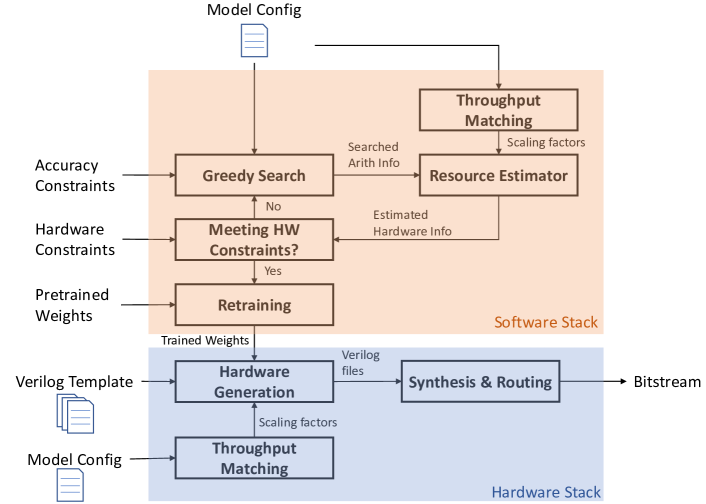
Figure 2: Framework overview for generating the accelerator for a targeting network on a particular dataset.

figure]fig:framework_overview

IV-A Framework Overview

LABEL:fig:framework_overview shows an overview of Tomato. The framework starts with an automated design process in software which uses the algorithm in Section III-C to explore the choices of fixed-point and shift arithmetics with varying precisions on the pre-trained CNN model. It then produces optimized models that are fully quantized while satisfying the accuracy constraints. In the exploration procedure, it iteratively uses an accurate hardware resource estimator to provide fast statistics of the hardware costs and minimize the costs for the searched models. The cost (latency, LUT and BRAM usage) is estimated using analytical models generated from post synthesis results for a wide range of module parameters The final optimized CNN model is then fine-tuned on the original training dataset to minimize accuracy degradation.

It is notable that from the optimized model, Tomato generates dedicated compute engines for each convolutional layer. As we have mentioned earlier, the compute engines are connected in a pipeline, each takes a stream of inputs and produces a stream of outputs. The isolated compute engines can thus have the freedom to use different quantizations with individual bitwidths. To minimize hardware utilization, layers that exceed throughput requirements can be folded (i.e. only partially unrolled) to share individual processing elements temporally. In Section IV-C we explain how each layer can temporally share its resources, and how we design the throughput matching block (Section IV-D) to automatically compute the optimal unroll factors required to parallelize each layer which minimizes stalls and idle circuits. Finally, the framework generates SystemVerilog output describing the hardware implementation of the input model, which is in turn synthesized into circuits with fine-tuned weights.

IV-B Macro-Architecture

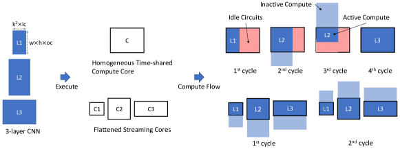
Figure 3: An illustration of computation flows on executing three layers of convolutions ($L_{1},L_{2},L_{3}$) at different clock cycles. $C$ represent a large homogeneous compute core and $C_{1},C_{2},C_{3}$ are smaller compute cores in a flattened streaming architecture. The rectangle block of each convolution layer represents input dimensions of a convolution flattened in 2D. k, ic, oc, w, h are kernel size, input/output channels, width and height of input feature feature maps respectively.

figure]fig:arch_overview

LABEL:fig:arch_overview shows the architecture differences between a normal homogeneous core style accelerator and our generated flattened streaming cores. In the flattened streaming cores, each convolution has its dedicated compute engine, slide buffer and weight buffer. Since the hardware is generated solely for the targeted CNN and each compute core is dedicated for a particular layer, with a suitable strategy to parallelize compute, the generated hardware can reach very high compute efficiency and have minimal idle hardware. In fact, in our measurements, compute unit utilization is constantly high at around $84\%$.

We employ barrel shifters or short fixed-point multipliers in the convolution compute engines. The weights are packed into BRAMs, and streamed into the convolution compute engines. Since weights are quantized as low precision shift or fixed-point values, the shorter bitwidths directly translates into lower BRAM usage. Additionally, because memory ports can be time-shared, this in turn reduces the number of BRAMs required.

IV-C Micro-Architecture: Roll-Unrolled Convolutions

In this section, we introduce the roll-unrolled convolution compute core, this is designed to minimize hardware costs when input and output data rates permit. As an example, we consider a convolution layer with a kernel size of $K$, which takes as input feature maps ${\mathbf{x}}$ of shape $H\times W\times C$, and produces output feature maps ${\mathbf{y}}$ of shape $H^{\prime}\times W^{\prime}\times C^{\prime}$ with $H^{\prime}$ and $W^{\prime}$ depending on the stride size and padding length. In addition, it is noteworthy that a convolution with a stride size of 1 can produce pixels in the output feature maps at the same rate of it taking input pixels. A convolution with a stride size of 2, however, produces an output pixel 4 times slower than it can consume an input pixel. Layers in a convolutional network can therefore process their feature maps at an exponentially slower rate as more proceeding layers are strided, and in turn have greater opportunities to reuse data-paths. By way of illustration, assuming the input image is fed at a rate of 1 cycle per pixel, the input/output throughput rates of each layer in a MobileNet-V1 can be found in the last column of Table I.

In order to maximize a layer’s utilization and minimize hardware costs, rather than introducing stall cycles, we introduce two unroll factors, $U$ and $U^{\prime}$, for input and output channels respectively. We partially roll input channel dimension $C$ into $U$-sized blocks to save hardware resource. We still accumulate $C^{\prime}$ values in parallel for ${\mathbf{y}}$. In other words, all $C^{\prime}$ channels of a pixel of the output feature maps are unrolled and computed concurrently. Fully unrolling output channels during multiplication and accumulation is essential to allow stall-free computation. Finally, output channels are rolled after accumulation to $U^{\prime}$-sized blocks for batch normalization. Fused batch normalization and ReLU operations are time-shared for $U^{\prime}$ output channels, as the next layer has an input block size equal to $U^{\prime}$. As we process all input channels $C$ in blocks of size $U$, we use only $U\times C^{\prime}$, instead of $C\times C^{\prime}$ parallel shift-accumulate or multiply-accumulate units, requiring $\left\lceil\frac{C}{U}\right\rceil$ cycles to complete the computation of a single pixel of all output channels, as shown in Figure 4.

Tomato does not use roll-unrolled in depthwise convolutions. Figure 5 shows the computation pattern for depthwise convolutions. In contrast to normal convolutions, depthwise convolutions are channel-wise operations, i.e. they do not exchange information across channels. By rolling input channels in depthwise layers, the generated outputs are also rolled, different from the normal roll-unrolled compute pattern. In this way, we exactly match the throughput of incoming and upcoming computations while minimizing resource utilization. Each parallel adder tree sums up $K^{2}$ values and is fully pipelined, where $K$ is the kernel size.

Roll-unrolled should not be confused with loop tiling. Loop tiling reorders the access pattern so that it is more friendly to CPU caches and DRAM bandwidth utilization in systolic array based CNN accelerators. As Tomato pipelines multiple frames instead of batching them, we did not change the access pattern. The purpose of rolling and unrolling in Tomato’s streaming cores are to minimize hardware and provides a stall-free computation dataflow, a fundamentally different objective.

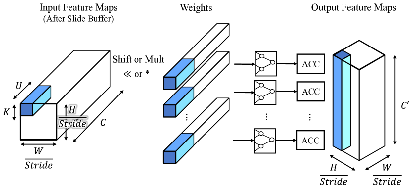
Figure 4: An illustration of roll-unrolled computation for normal convolution (including pointwise convolution): blue indicates data elements computed in a single cycle.

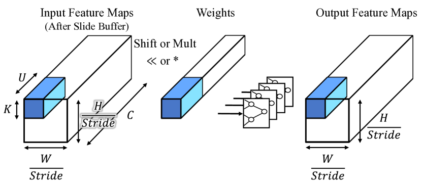
Figure 5: An illustration of depthwise convolution: blue indicates data elements computed in a single cycle.

IV-D Striding and Rolling: Matching the Throughput

By adjusting the unroll factors $U$ and $U^{\prime}$, the framework smartly matches the throughput between convolution layers with different channel counts and stridings for higher efficiency. The only free parameter now is the input pixel rate at the very first layer of the CNN. The input pixel rate determines how many pixels of an input image are fed into the accelerator at each clock cycle. For instance, an input rate of $\frac{1}{32}$ means we consume $1$ input pixel in $32$ clock cycles. The choice of the input pixel rate directly impacts the trade-off between performance and the hardware resources required. If this input pixel rate is $1$, the generated hardware is optimized for performance, fully-pipelined, and never stalls the input pixel steam. When the input pixel rate decreases, because of the automatic matching, unroll factors of all subsequent convolution layers decrease and the generated hardware thus utilizes fewer resources but has an increased latency.

TABLE I: Unrolling factors $U$ and $U^{\prime}$ are generated by the throughput matcher for MobileNet-V1, depending on the input and output channel counts ($C$, $C^{\prime}$), and the stride of each convolution. dw and pw are depthwise and pointwise convolution. s1 and s2 represents strides are 1 and 2.

Types	$\mathbf{C\text{ / }C^{\prime}}$	$\mathbf{U\text{ / }U^{\prime}}$	$\mathbf{\frac{C}{U}\text{ / }\frac{C^{\prime}}{U^{\prime}}}$
Conv / s2	3 / 32	3 / 8	1 / 4
Conv dw / s1	32 / 32	8 / 8	4 / 4
Conv pw / s1	32 / 64	8 / 16	4 / 4
Conv dw / s2	64 / 64	16 / 4	4 / 16
Conv pw / s1	64 / 128	4 / 8	16 / 16
Conv dw / s1	128 / 128	8 / 8	16 / 16
Conv pw / s1	128 / 128	8 / 8	16 / 16
Conv dw / s2	128 / 128	8 / 2	16 / 64
Conv pw / s1	128 / 256	2 / 4	64 / 64
Conv dw / s1	256 / 256	4 / 4	64 / 64
Conv pw / s1	256 / 256	4 / 4	64 / 64
Conv dw / s2	256 / 256	4 / 1	64 / 256
Conv pw / s1	256 / 512	1 / 2	256 / 256
Conv dw / s1	512 / 512	2 / 2	256 / 256
Conv pw / s1	512 / 512	2 / 2	256 / 256
Conv dw / s2	512 / 512	2 / 1	256 / 512
Conv pw / s1	512 / 1024	1 / 1	512 / 1024
Conv dw / s1	1024 / 1024	1 / 1	1024 / 1024
Conv pw / s1	1024 / 1024	1 / 1	1024 / 1024
Avg Pool / s1	1024 / 1024	1 / 1	1024 / 1024
FC / s1	1024 / 1000	1 / 1	1024 / 1000

We now explain how the automated throughput matching works. The framework utilizes the classic sliding window design — one pixel of a output feature map is produced once all pixels of the sliding window on input feature maps have arrived [2]. The input stream and output stream of strided convolutions, however, can have different input and output rates. For instance, when the stride size is 2, the output stream is then 4 times slower than the input stream (striding occurs in the two spatial dimensions). Table I shows the unrolling factors $U$ and $U^{\prime}$ that the framework picked for each convolution in MobileNet-V1 when choosing the input pixel rate to be $1$. Here, for each pixel, $\frac{C}{U}$ represents the number of clock cycles required to iterate over all input channel values, and $\frac{C^{\prime}}{U^{\prime}}$ is the number of cycles required to finish generating all output channel values. Taking the second depthwise convolution layer as an example, this layer has a stride size of 2 and the framework rolls computations on the output channel side by a factor of $\frac{C^{\prime}}{U^{\prime}}=16$ so that $U^{\prime}=4$ values of each output channel are computed concurrently. Finally, all of the unrolling information is provided to the hardware templates in order to instantiate the appropriate hardware.

IV-E Batch Normalization and Rounding

Each convolved output has an inflated precision as mentioned in Section IV-C, and we subsequently apply BN on these values. As mentioned in Section III, BN is fused and quantized to become a channel-wise affine transformation with fixed-point arithmetic. We therefore use the on-chip DSP elements to perform fixed-point multiplications and rounding after BN. Since we roll computations in output channel dimensions, the number of multiplications required by BN is also significantly reduced by sharing. It is notable that weights share a layer-wise bias value (Equation 1, Equation 2). The weights bias is included in the rounding after BN, as it simply moves the binary point. The final results are then rounded to 8-bit fixed-point values with a 5-bit fractional width.

V Results

TABLE II: Summary of tested networks on the Tomato. IPP stands for input pixel rate.

Network IPP Platform Perf Metrics LUTs Registers BRAMs DSPs Top-1 Top-5 Size MobileNet-V1 1 Intel Stratix 10 Frequency 156 MHz Used 926 k 583 k 1430 297 Orig. 70.71 89.53 33.92 MB Latency 358 µs Total 1866 k 3732 k 11721 5760 Quant. 68.02 88.02 16.1 MB Throughput 3109 fps Ratio 49% 15% 12% 5% $\mathbf{\Delta}$ -2.69 -1.51 2.11$\times$ CifarNet $\frac{1}{32}$ Intel Stratix V Frequency 207 MHz Used 304 k 280 k 771 84 Orig. 91.37 99.68 4.94 MB Latency 261 µs Total 469 k 939 k 2.56 k 256 Quant. 91.06 99.58 520 kB Throughput 6317 fps Ratio 64% 29% 30% 32% $\mathbf{\Delta}$ -0.31 -0.10 9.73$\times$ CifarNet $\frac{1}{288}$ Intel Cyclone V Frequency 116 MHz Used 102 k 84.7 k 715 82 Orig. 91.37 99.68 4.94 MB Latency 4.01 ms Total 227 k 454 k 1.22 k 342 Quant. 91.06 99.58 520 kB Throughput 393 fps Ratio 44% 18% 58% 24% $\mathbf{\Delta}$ -0.31 -0.10 9.73$\times$ FashionNet $\frac{1}{9}$ Xilinx Artix 7 Frequency 98 MHz Used 49.3 k 32.7 k 40 240 Orig. 91.79 99.67 443 kB Latency 138 µs Total 63.4 k 127 k 135 240 Quant. 91.57 99.56 65.3 kB Throughput 13.9 kfps Ratio 77% 25% 29% 100% $\mathbf{\Delta}$ -0.22 -0.11 6.78$\times$

V-A Implementation Setup

In this paper, we report results for automatically generated hardware implementations for three distinct networks, each optimized for a different dataset. We use CifarNet [44], an 8-layer CNN with 1.30 M parameters and 174 M multiply-accumulates on the CIFAR-10 dataset [17], MobileNet-V1 [11] on the ImageNet dataset [6] and a customized 5-layer CNN (FashionNet) for the Fashion MNIST dataset [37]. The first two networks are relatively large, but the last network is small. We use MobileNet-V1 design as a comparison to showcase the performance achieved from this hardware and software co-design workflow in comparison to other published accelerators. The hardware part (SystemVerilog output) is generated automatically using templates by the Tomato framework. We use Synplify Premier DP for synthesis and post-synthesis timing analysis. We verified that our designs are actually implementable on FPGA by using Xilinx Vivado to place and route the full-size MobileNet design.

V-B Resource Utilization

For MobileNet, our design is fully-pipelined and never stalls the input stream ($\frac{\text{\#OPs}}{\text{\#OPs/cycle}}=224\times 224$). Note that $224\times 224$ is the input image size and this means the accelerator consumes an entire image in exactly $224\times 224$ clock cycles. We utilise 84% of our 13479 compute units (shift-and-add or multiply-and-add) on every clock cycle. The high utilization rate of the hardware translates to high activity ratio in the circuits since most components are active all the time. This fully quantized MobileNet found by Algorithm 1 uses 3-bit shift weights in its pointwise layers, and fixed-point weights in its depthwise layers with precisions ranging from 3 to 7.

Table II shows the total amount of hardware utilized for the generated accelerators for all networks on different devices. We generate a MobileNet design with the input pixel rate set to $1$ for best performance (achieving 3109 FPS on an Intel Stratix 10). The proposed workflow is a scalable one since we can adjust the input pixel rate to control a trade-off between performance and hardware utilization. CifarNet results in Table II show how it is possible to target a small FPGA device (Cyclone V) by adjusting this factor to $\frac{1}{288}$. The results suggest a $3\times$ reduction in LUT usage compared to the design when the input pixel rate is set to $\frac{1}{32}$. We also observe an increase in latency, but part of the increase attributes to the frequency differences running on various devices. On the other hand, if provided with a small network (FashionNet), the proposed framework generates hardware that classifies at a latency of $0.14$ms on a very small FPGA device. The quantized FashionNet uses 3-bit shift quantization in the most resource-intensive third layer, and the remaining layers use fixed-point weights with bit-widths from 5 to 7. Although FashionNet is small, it is a good example of a specialized network produced for resource constrained edge devices; other examples include emotion recognition [3].

We explore in Figure 6 the optimized CifarNets obtained with Algorithm 1 (denoted by the “hybrid” points) and compare the results against shift (“shift”) and fixed-point (“fixed”) models with all layers sharing the same bit-widths ranging from 3 to 8. To explore the trade-off between top-1 error rates and resources, we ran Algorithm 1 $20$ times by respectively taking as inputs the accuracy budget values $\alpha_{\mathrm{budget}}$ ranging from $80\%$ to $100\%$ at $1\%$ increments. Here $h_{\mathrm{budget}}$ is set to $0$ as we always minimize the resource utilization. We constrain each layer to use either shift or fixed-point quantized weights and choose a bit-width ranging from 3 to 8. Additionally, $E=0$ meaning that we skip the fine-tuning process; without fine-tuning the accuracies are sub-optimal but the search process above can complete within 1 hour. Figure 6(a) shows the trade-off between resource utilization and top-1 errors under the same throughput constraints. Figure 6(b) further varies the throughput scaling of the optimized results, and shows that when synthesized into circuits, the the optimized models (“hybrid”) consistently outperforms models (“shift” and “hybrid”) with either shift or fixed-point quantization under the same bit-width applied across all layer weights. Finally, Figure 6(c) illustrates all results found by the three methods and the trade-off relationship between top-1 error rates and resource-latency products.

Hybrid quantization reduces accuracy degradations but improves model compression rates by utilizing multi-precision multi-arithmetic convolutions. Importantly, we consider the ImageNet [6] classification task for MobileNet. This challenging dataset leaves less headroom for compression techniques. The classification results achieved on this large dataset using a relatively compact network proves that the workflow is also robust on other cases where the model is over-provisioned on the target dataset.

TABLE III: A comparison of CNN inference performance on FPGA and GPU platforms. The quantization of weights and activations are on the left. Target platform, frequency, latency, throughput and arithmetic performance are on the right. Metrics with ^∗ are our best-case estimations as they are not mentioned in the original papers. Note VGG16 has a similar top-5 accuracy to MobileNet-V1 when neither is quantized, many of the works below do not report ImageNet accuracies after quantization.

		Quantisation(s)		Platform	Frequency (MHz)	Latency (ms)	Throughput (FPS)	Arithmetic perf. (GOP/s)
	Implementation	Weights	Acts
VGG16	Throughput-Opt [33]	FXP8	FXP16	Intel Stratix V	120	262.9	3.8∗	117.8
	fpgaConvNet [34]	FXP16	FXP16	Xilinx Zynq XC7Z045	125	197∗	5.07	156
	Angel-Eye [9]	BFP8	BFP8	Xilinx Zynq XC7Z045	150	163∗	6.12∗	188
	Going Deeper [25]	FXP16	FXP16	Xilinx Zynq XC7Z045	150	224∗	4.45	137
	Shen et al. [31]	FXP16	FXP16	Xilinx Virtex US XCVU440	200	49.1	26.7	821
	HARPv2 [23]	BIN	BIN	Intel HARPv2	–	8.77∗	114	3500
	GPU [23]	FP32	FP32	Nvidia Titan X	–	–	121	3590
MobileNet	Ours	Mixed	FXP8	Intel Stratix 10	156	0.32	3109	3536
	Ours	Mixed	FXP8	Xilinx Virtex US+ XCVU9P	125	0.40	2491	2833
	Zhao et al. [41]	FXP16	FXP16	Intel Stratix V	200	0.88	1131	1287
	Zhao et al. [42]	FXP8	FXP8	Intel Stratix V	150	4.33	231	264
	GPU	FP32	FP32	Nvidia GTX 1080Ti	–	279.4	515	586

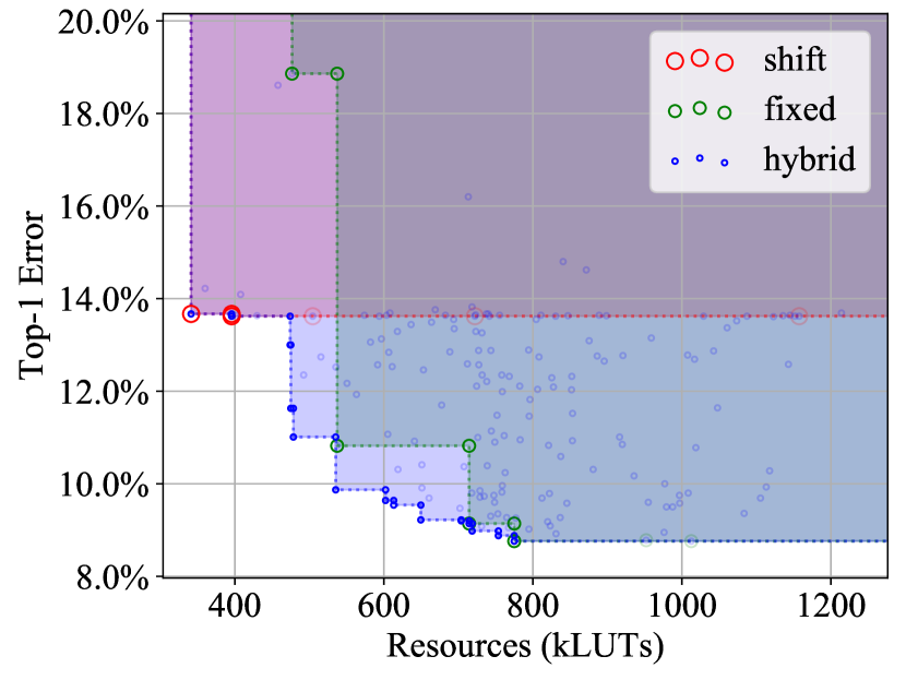
(a) Number of LUTs vs. top-1 error under the same $\frac{1}{32}$ scaling and the same throughput.

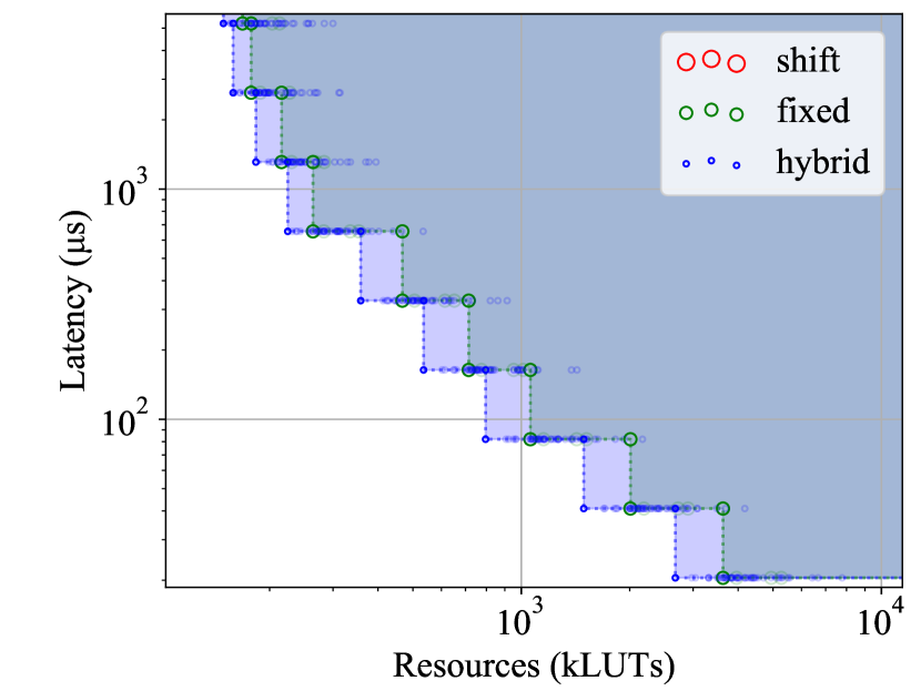
(b) Number of LUTs vs. latency for models with $\leq 10\%$ top-1 errors.

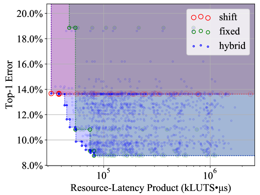
(c) Error vs. area-latency product for all optimized models.

Figure 6: A case study of trade-off options among hardware utilization (LUTs), performance (latency) and model accuracy (top-1 error rate) before fine-tuning, targeting a clock frequency of $200$ MHz. The LUTs and latency numbers are from the hardware estimator. Here, “shift” and “fixed” respectively indicate using the same shift and fixed-point quantization method across all layers with the same weight precisions. The “hybrid” points are optimized by Algorithm 1. The area shaded in red, green and blue respectively denote the 2D Pareto frontier of “shift”, “fixed” and “hybrid” optimized results.

V-C Performance Evaluation

We compare the MobileNet-V1 design generated by our framework with existing FPGA accelerators in Table III. This comparison only considers networks in the ImageNet dataset that achieves greater than $70\%$ top-1 accuracy when not quantized. The computer vision community spends a significant amount of effort in optimizing model architecture, we note that it is important to generate results for the latest models as they offer the best accuracy/cost trade offs. Results for older models in terms of GOP/s can be misleading.

Our design is different from most existing designs examined in Table III in the following ways. First, our framework exploits hybrid quantization to minimize the impact of quantization errors. Second, using the throughput scaling trick, the amount of hardware required is reduced significantly. Most of the examined designs rely on a high DRAM bandwidth with a large monolithic compute core. As discussed previously, a large compute core cannot explore multi-precision and multi-arithmetic quantizations and struggles to fully utilize compute units on convolutions with varying channel counts, kernel sizes and input feature sizes. Tomato generated designs compute various layers concurrently and quantize each layer differently, thus achieving a very high utilization of our compute units and to operate at around 3.5 TOPs/s on Stratix 10. Note that, for accelerators that we compare against, the arithmetic performance reported in Table III considers the peak performance assuming unbounded DRAM bandwidth. In reality, such designs can easily be limited by the available memory bandwidth. In contrast, this is not a concern in our design as all weights and activations are held on the FPGA. Additionally, our design has a high throughput since operations rarely stall. Designs proposed by Bai et al. [2] and Zhao et al.  [41] have to execute computations in a layer-wise fashion, and thus operations in the next layer only executes when the current layer finishes. In our framework, similar to Shen et al. [32], computations in different layers happen concurrently in the same pipeline stage while later layers never stall earlier layers. Moreover, consecutive image inputs can be fully pipelined, because we utilize streaming sliding windows. These features help us to achieve high throughput compared to other designs (Table III). The proposed workflow avoids complex and time-consuming design space exploration as necessary in many compared FPGA accelerators [2, 42].

In terms of performance, our design achieves a higher throughput and a lower latency compared to all designs (as listed in Table III). We notice that most CNN accelerators report theoretical upper bounds for arithmetic performance and throughput. In terms of latency, the numbers are reported optimistically assuming DRAM accesses cause no stalls. In our design, since we stream in pixels of the input image, the computation pattern differs from most existing designs. The reported values in Table III represents our true performance and make no assumptions regarding DRAM bandwidth. Our system automatically produces an implementation of MobileNet for the Stratix 10 FPGA that outperforms Zhao et al. [41] by $2.44\times$ in latency and $3.52\times$ in throughput.

V-D Multi-FPGA Acceleration

The flattened streaming style employed by Tomato makes it easy to partition the generated design across multiple FPGAs This feature makes Tomato highly scalable with respect to network sizes and/or FPGA sizes. We demonstrate in this section an example of partitioning MobileNet-V1 onto two Stratix V FPGAs, connected through enhanced small form-factor pluggable (SFP+) interfaces. We present the performance results in comparison to Zhang et al. [38] in Table IV, and the detailed hardware utilization information in Table V. The latency is not penalised thanks to the low latency of SFP+, which contributes only a $0.0013$ms latency overhead.

The simple case study of partitioning the same MobileNet-V1 design to two devices demonstrates that, first, Tomato generated designs are scalable from single to multi-FPGAs; second, aiming accelerating new network architectures with mixed quantizations bring significant improvements in accuracies, latency and throughput.

TABLE IV: Multi-FPGA acceleration of CNNs. MBNet represents MobileNet, VGG-D and VGG-E are both VGG16 based networks but different configurations, one is latency oriented and one is throughput oriented [38].

Network	Acc (%)	#Device	Lat (ms)	Tpt (GOPs)
MbNet-V1 (ours)	68.02	2 Stratix V	0.32	3536
VGG-D [38]	66.52	2 VX690t	200.9	203
VGG-E [38]	66.51	7 VX690t	151.8	1280

TABLE V: Multi-FPGA hardware utilization.

Device No	Frequency	LUTs	Regs	BRAM	DSP
0	156MHz	362.7k	278.8k	828	256
1	156MHz	345.9k	303.6k	598	31

VI Conclusion

In this paper, we presented a hardware-software co-design workflow to automatically generate high-performance CNN accelerators. The workflow is able to quantize weights to both fixed-point and shift values at various precisions, and keeps activations to fixed-point numbers. In addition, it transforms batch normalization to simple affine operations with fixed-point scaling and offset factors. In hardware, the framework utilizes the Roll-Unrolled compute pattern and provides flexibility in rolling computations in the channel dimension. As a result, the guided rolling minimizes computation while keeping the input stream stall-free. The results showed state-of-the-art performance in terms of model accuracy, latency and throughput. The implemented accelerator for MobileNet is fully pipelined with sub-millisecond latency (0.32ms) and is able to classify at around 3000 frames per second.

References

- [1] M. Alwani, H. Chen, M. Ferdman, and P. Milder. Fused-layer CNN accelerators. In The 49th Annual IEEE/ACM International Symposium on Microarchitecture, 2016.
- [2] L. Bai, Y. Zhao, and X. Huang. A CNN accelerator on FPGA using depthwise separable convolution. IEEE Transactions on Circuits and Systems II: Express Briefs, 2018.
- [3] P.-L. Carrier, A. Courville, I. J. Goodfellow, M. Mirza, and Y. Bengio. FER-2013 face database. Technical report, 2013.
- [4] Y.-H. Chen, T. Krishna, J. S. Emer, and V. Sze. Eyeriss: An energy-efficient reconfigurable accelerator for deep convolutional neural networks. IEEE Journal of Solid-State Circuits, 2016.
- [5] M. Courbariaux, Y. Bengio, and J.-P. David. Training deep neural networks with low precision multiplications. In International Conference on Learning Representations, 2015.
- [6] J. Deng, W. Dong, R. Socher, L.-J. Li, K. Li, and L. Fei-Fei. ImageNet: A large-scale hierarchical image database. In IEEE Conference on Computer Vision and Pattern Recognition, 2009.
- [7] J. Fowers, K. Ovtcharov, M. Papamichael, T. Massengill, M. Liu, D. Lo, S. Alkalay, M. Haselman, L. Adams, M. Ghandi, et al. A configurable cloud-scale DNN processor for real-time ai. In 45th Annual International Symposium on Computer Architecture, 2018.
- [8] X. Gao, Y. Zhao, L. Dudziak, R. Mullins, and C.-z. Xu. Dynamic channel pruning: Feature boosting and suppression. 2019.
- [9] K. Guo, L. Sui, J. Qiu, S. Yao, S. Han, Y. Wang, and H. Yang. Angel-Eye: A complete design flow for mapping CNN onto customized hardware. In IEEE Computer Society Annual Symposium on VLSI, 2016.
- [10] Y. He, X. Zhang, and J. Sun. Channel pruning for accelerating very deep neural networks. In International Conference on Computer Vision (ICCV), 2017.
- [11] A. G. Howard, M. Zhu, B. Chen, D. Kalenichenko, W. Wang, T. Weyand, M. Andreetto, and H. Adam. MobileNets: Efficient convolutional neural networks for mobile vision applications. 2017.
- [12] I. Hubara, M. Courbariaux, D. Soudry, R. El-Yaniv, and Y. Bengio. Binarized neural networks. In Advances in Neural Information Processing Systems. 2016.
- [13] I. Hubara, M. Courbariaux, D. Soudry, R. El-Yaniv, and Y. Bengio. Quantized neural networks: Training neural networks with low precision weights and activations. J. Mach. Learn. Res., 2017.
- [14] K. Hwang and W. Sung. Fixed-point feedforward deep neural network design using weights , , and . In Signal Processing Systems, 2014.
- [15] S. Ioffe and C. Szegedy. Batch normalization: Accelerating deep network training by reducing internal covariate shift. arXiv preprint arXiv:1502.03167, 2015.
- [16] R. Krishnamoorthi. Quantizing deep convolutional networks for efficient inference: A whitepaper. arXiv preprint arXiv:1806.08342, 2018.
- [17] A. Krizhevsky, V. Nair, and G. Hinton. The CIFAR-10 and CIFAR-100 datasets. http://www.cs.toronto.edu/ kriz/cifar.html, 2014.
- [18] A. Krizhevsky, I. Sutskever, and G. E. Hinton. ImageNet classification with deep convolutional neural networks. In Advances in Neural Information Processing Systems 25. 2012.
- [19] F. Li, B. Zhang, and B. Liu. Ternary weight networks. arXiv preprint arXiv:1605.04711, 2016.
- [20] S. Liang, S. Yin, L. Liu, W. Luk, and S. Wei. FP-BNN: Binarized neural network on FPGA. Neurocomput., 2018.
- [21] W. Liu, D. Anguelov, D. Erhan, C. Szegedy, S. Reed, C.-Y. Fu, and A. C. Berg. SSD: Single shot multibox detector. In European conference on computer vision, 2016.
- [22] A. Mollahosseini, D. Chan, and M. H. Mahoor. Going deeper in facial expression recognition using deep neural networks. In 2016 IEEE winter conference on applications of computer vision (WACV), 2016.
- [23] D. Moss, S. Krishnan, E. Nurvitadhi, P. Ratuszniak, C. Johnson, J. Sim, A. Mishra, D. Marr, S. Subhaschandra, and P. H. W. Leong. A customizable matrix multiplication framework for the Intel HARPv2 Xeon + FPGA platform. In ACM/SIGDA International Symposium on Field-Programmable Gate Arrays, 2018.
- [24] D. C. Plaut and G. E. Hinton. Learning sets of filters using back-propagation. Computer Speech & Language, 1987.
- [25] J. Qiu, J. Wang, S. Yao, K. Guo, B. Li, E. Zhou, J. Yu, T. Tang, N. Xu, and S. Song. Going deeper with embedded FPGA platform for convolutional neural network. In ACM/SIGDA International Symposium on Field-Programmable Gate Arrays, 2016.
- [26] M. Rastegari, V. Ordonez, J. Redmon, and A. Farhadi. XNOR-Net: ImageNet classification using binary convolutional neural networks. In ECCV, 2016.
- [27] M. Samragh, M. Ghasemzadeh, and F. Koushanfar. Customizing neural networks for efficient FPGA implementation. In 2017 IEEE 25th Annual International Symposium on Field-Programmable Custom Computing Machines (FCCM), 2017.
- [28] S. S. Sarwar, S. Venkataramani, A. Raghunathan, and K. Roy. Multiplier-less artificial neurons exploiting error resiliency for energy-efficient neural computing. In 2016 Design, Automation Test in Europe Conference Exhibition (DATE), 2016.
- [29] S. Sharify, A. D. Lascorz, M. Mahmoud, M. Nikolic, K. Siu, D. M. Stuart, Z. Poulos, and A. Moshovos. Laconic deep learning inference acceleration. In Proceedings of the 46th International Symposium on Computer Architecture, ISCA ’19, 2019.
- [30] H. Sharma, J. Park, N. Suda, L. Lai, B. Chau, V. Chandra, and H. Esmaeilzadeh. Bit fusion: Bit-level dynamically composable architecture for accelerating deep neural networks. In Proceedings of the 45th Annual International Symposium on Computer Architecture, 2018.
- [31] J. Shen, Y. Huang, Z. Wang, Y. Qiao, M. Wen, and C. Zhang. Towards a uniform template-based architecture for accelerating 2D and 3D CNNs on FPGA. In ACM/SIGDA International Symposium on Field-Programmable Gate Arrays, 2018.
- [32] Y. Shen, M. Ferdman, and P. Milder. Maximizing CNN accelerator efficiency through resource partitioning. In 2017 ACM/IEEE 44th Annual International Symposium on Computer Architecture (ISCA), 2017.
- [33] N. Suda, V. Chandra, G. Dasika, A. Mohanty, Y. Ma, S. Vrudhula, J.-s. Seo, and Y. Cao. Throughput-optimized OpenCL-based FPGA accelerator for large-scale convolutional neural networks. In Proceedings of the 2016 ACM/SIGDA International Symposium on Field-Programmable Gate Arrays, 2016.
- [34] S. I. Venieris and C.-S. Bouganis. fpgaConvNet: A framework for mapping convolutional neural networks on FPGAs. In IEEE International Symposium on Field-Programmable Custom Computing Machines, 2016.
- [35] E. Wang, J. J. Davis, P. Y. Cheung, and G. A. Constantinides. LUTNet: Rethinking Inference in FPGA Soft Logic. In IEEE International Symposium on Field-programmable Custom Computing Machines, 2019.
- [36] E. Wang, J. J. Davis, R. Zhao, H.-C. Ng, X. Niu, W. Luk, P. Y. K. Cheung, and G. A. Constantinides. Deep Neural Network Approximation for Custom Hardware: Where We’ve Been, Where We’re Going. ACM Computing Surveys, (2), 2019.
- [37] H. Xiao, K. Rasul, and R. Vollgraf. Fashion-MNIST: a novel image dataset for benchmarking machine learning algorithms. arXiv preprint, 2017.
- [38] C. Zhang, D. Wu, J. Sun, G. Sun, G. Luo, and J. Cong. Energy-efficient cnn implementation on a deeply pipelined fpga cluster. In Proceedings of the 2016 International Symposium on Low Power Electronics and Design, 2016.
- [39] X. Zhang, J. Wang, C. Zhu, Y. Lin, J. Xiong, W.-m. Hwu, and D. Chen. DNNBuilder: an automated tool for building high-performance dnn hardware accelerators for fpgas. In Proceedings of the International Conference on Computer-Aided Design, page 56. ACM, 2018.
- [40] X. Zhang, X. Zhou, M. Lin, and J. Sun. Shufflenet: An extremely efficient convolutional neural network for mobile devices. In IEEE Conference on Computer Vision and Pattern Recognition, 2018.
- [41] R. Zhao, H.-C. Ng, W. Luk, and X. Niu. Towards efficient convolutional neural network for domain-specific applications on FPGA. arXiv preprint, 2018.
- [42] R. Zhao, X. Niu, and W. Luk. Automatic optimising CNN with depthwise separable convolution on FPGA: (abstact only). In ACM/SIGDA International Symposium on Field-Programmable Gate Arrays, 2018.
- [43] Y. Zhao, X. Gao, D. Bates, R. Mullins, and C.-Z. Xu. Focused quantization for sparse CNNs. In Advances in Neural Information Processing Systems, 2019.
- [44] Y. Zhao, X. Gao, R. Mullins, and C. Xu. Mayo: A framework for auto-generating hardware friendly deep neural networks. In Proceedings of the 2Nd International Workshop on Embedded and Mobile Deep Learning, EMDL’18, 2018.
- [45] A. Zhou, A. Yao, Y. Guo, L. Xu, and Y. Chen. Incremental network quantization: Towards lossless CNNs with low-precision weights. International Conference on Learning Representations (ICLR), 2017.
- [46] C. Zhu, S. Han, H. Mao, and W. J. Dally. Trained ternary quantization. In International Conference on Learning Representations, 2017.