Accurate quadrature of nearly singular line integrals in two and three dimensions by singularity swapping

Abstract

The method of Helsing and co-workers evaluates Laplace and related layer potentials generated by a panel (composite) quadrature on a curve, efficiently and with high-order accuracy for arbitrarily close targets. Since it exploits complex analysis, its use has been restricted to two dimensions (2D). We first explain its loss of accuracy as panels become curved, using a classical complex approximation result of Walsh that can be interpreted as “electrostatic shielding” of a Schwarz singularity. We then introduce a variant that swaps the target singularity for one at its complexified parameter preimage; in the latter space the panel is flat, hence the convergence rate can be much higher. The preimage is found robustly by Newton iteration. This idea also enables, for the first time, a near-singular quadrature for potentials generated by smooth curves in 3D, building on recurrences of Tornberg–Gustavsson. We apply this to accurate evaluation of the Stokes flow near to a curved filament in the slender body approximation. Our 3D method is several times more efficient (both in terms of kernel evaluations, and in speed in a C implementation) than the only existing alternative, namely, adaptive integration.

1 Introduction

Integral equation methods enable efficient numerical solutions to piecewise-constant coefficient elliptic boundary value problems, by representing the solution as a layer potential generated by a so-called “density” function defined on a lower-dimensional source geometry [4, 32]. This work is concerned with accurate evaluation of such layer potentials close to their source, when this source is a one-dimensional curve embedded in 2D or 3D space. In 2D, this is a common occurrence: the curve is the boundary of the computational domain or an interface between different materials. In 3D, such line integrals represent the fluid velocity in non-local slender-body theory (SBT) for filaments in a viscous (Stokes) flow [29, 27, 17], and also may represent the fields in the solution of electrostatic [43] or elecromagnetic [11] response of thin wire conductors. Applications of the former include simulation of straight [46], flexible [47, 36] or closed-loop [34] fiber suspensions in fluids. SBT has recently been placed on a more rigorous footing as the small-radius asymptotic limit of a surface boundary integral formulation [34, 35, 31]. In this work we focus on non-oscillatory kernels arising from Laplace (electrostatic) and Stokes applications, although we expect that by singularity splitting (e.g. [20]) the methods we present could be adapted for oscillatory or Yukawa kernels.

For numerical solution, the density function must first be discretized [45, 32]. A variety of methods are used in practice. If the geometry is smooth enough, and the interacting objects are far enough away that the density is also smooth, then a non-adaptive density representation is sufficient. Such representations include low-order splines on uniform grids [47], global spectral discretization by the periodic trapezoid rule for closed curves [32, 18, 6], and, for open curves, global Chebychev [11, 36] or Legendre [46] expansions. However, if the density has regions where refinement is needed (such as corners or close interactions with other bodies), a composite (“panel”) scheme is better, as is common with Galerkin boundary-element methods [45]. On each panel a high-order representation (such as the Lagrange basis for a set of Gauss–Legendre nodes) is used; panels may then be split in either a graded [45, 25, 37] or adaptive [38, 42, 51] fashion.

Our goal is accurate and efficient evaluation of the potential due a density given on a panel, at arbitrarily close target points. Not only is this crucial for accurate solution evaluation once the density is known, but is also key to constructing matrix elements for a Nyström or Galerkin solution [45, 32] in the case when curves are close to each other [24, 37, 6]. Specifically, let the panel $\Gamma$ be an open smooth curve in $\mathbb{R}^{d}$, where $d=2$ or $d=3$. We seek to evaluate the layer potential

$$u(\bm{x})=\int_{\Gamma}K(\bm{x},\bm{y})f(\bm{y})\operatorname{d\!}s(\bm{y}),\quad\bm{x}\notin\Gamma\subset\mathbb{R}^{d},$$ (1)

at the target point $\bm{x}\notin\Gamma$. Here the density $f$ is a smooth function defined on $\Gamma$, and $K$ is a kernel that has a singularity as $\bm{x}\to\bm{y}$. Letting $k$ denote some smooth (possibly tensor-valued) function on $\mathbb{R}^{d}$, in two dimensions the dominant singularity can be either logarithmic,

$$K(\bm{x},\bm{y})\sim k(\bm{x}-\bm{y})\log\mathinner{\!\left\lvert\bm{x}-\bm{y}\right\rvert},$$ (2)

or of power-law form

$$K(\bm{x},\bm{y})\sim\frac{k(\bm{x}-\bm{y})}{\mathinner{\!\left\lvert\bm{x}-\bm{y}\right\rvert}^{m}},\quad m=1,2,\dots,$$ (3)

where $m$ is generally even. In 3D only the latter form arises, for $m$ generally odd. We will assume that $\Gamma$ is described by the parametrization $\bm{g}\mathrel{\mathop{\mathchar 58\relax}}\mathbb{R}\to\mathbb{R}^{d}$ that maps the standard interval $[-1,1]$ to $\Gamma$,

$$\Gamma=\left\{\bm{g}(t)\mid t\in[-1,1]\right\}.$$ (4)

Thus the parametric form of the desired integral (1) is

$$u(\bm{x})=\int_{-1}^{1}K\left(\bm{x},\bm{g}(t)\right)\tilde{f}(t)\mathinner{\!\left\lvert\bm{g}^{\prime}(t)\right\rvert}\operatorname{d\!}t,\quad\bm{x}\notin\Gamma\subset\mathbb{R}^{d},$$ (5)

where $\tilde{f}(t)\mathrel{\mathop{\mathchar 58\relax}}=f(\bm{g}(t))$ is the pullback of the density to parameter space.

The difficulty of evaluation of a layer potential with given density is essentially controlled by the distance of the target point $\bm{x}$ from the curve. In particular, if $\bm{x}$ is far from $\Gamma$, the kernel $K(\bm{x},\bm{y})$ varies, as a function of $\bm{y}$, no more rapidly than the curve geometry itself. Thus a fixed quadrature rule, once it integrates accurately the product of density $f$ and any geometry functions (such as the “speed” $\mathinner{\!\left\lvert\bm{g}^{\prime}\right\rvert}$), is accurate for all such targets. Here, “far” can be quantified relative to the local quadrature node spacing $h$ and desired accuracy: e.g. in the 2D periodic trapezoid rule setting the distance should be around $(\log 10)h/2\pi\approx 0.37\,h$ times the desired number of correct digits (a slight extension of [7, Remark 2.6]). However, as $\bm{x}$ approaches $\Gamma$, $K(\bm{x},\bm{y})$ becomes increasingly non-smooth in the region where $\bm{y}$ is near $\bm{x}$, and any fixed quadrature scheme loses accuracy. This is often referred to as the layer potential integral being nearly singular.

There are several approaches to handling the nearly singular case. The most crude is to increase the number of nodes used to discretize the density; this has the obvious disadvantage of growing the linear system size beyond that needed to represent the density, wasting computation time and memory. Slightly less naive is to preserve the original discretization nodes, but interpolate from these nodes onto a refined quadrature scheme (with higher order or subdivided panels [47]) used only for potential evaluations. However, to handle arbitrarily close targets one has to refine the panels in an adaptive fashion, afresh for each target point. As a target approaches $\Gamma$ an increasing level of adaptive refinement is demanded. The large number of conditionals and interpolations needed in such a scheme can make it slow.

This has led to more sophisticated “special” rules which do not suffer as the target approaches the curve. They exploit properties of the PDE, or, in 2D, the relation of harmonic to analytic functions. In the 2D high-order setting, several important contributions have been made in the last decade, including panel-based kernel-split quadrature [24, 19, 37, 20, 22], globally compensated spectral quadrature [24, 6], quadrature by expansion (QBX) [7, 30, 49], harmonic density interpolation [40], and asymptotic expansion [12]. In 3D, little work has been done on high-order accurate evaluation of nearly singular line integrals. Many of the applications are in the context of active or passive filaments in viscous fluids, but the quadrature methods are limited to either using analytical formulae for straight segments [46], or regularizing the integrand using an artificial length scale [13, 26, 47].

In this paper, we propose a new panel-based quadrature method for nearly singular line integrals in both 2D and 3D. The method incurs no loss of efficiency for targets arbitrarily close to the curve. (Note that, in the 2D case it is usual for one-sided limits on $\Gamma$ to exist, but in 3D limits on $\Gamma$ do not generally exist.) Our method builds on the panel-based monomial recurrences introduced by Helsing–Ojala [24] and extended by Helsing and co-workers [19, 23, 21, 37] [22, Sec. 6], with a key difference that, instead of interpolating in the physical plane (which is associated with the complex plane), we interpolate in the (real) parametrization variable of the panel. Rather than exploiting Cauchy’s theorem in the spatial complex plane, the singularity is “swapped” by cancellation for one in the parameter plane; this requires a nearby root-finding search for the (analytic continuation of the) function describing the distance between the panel and the target. It builds on recent methods for computing quadrature error estimates in two dimensions [3]. We include a robust and efficient method for such root searches.

This new formulation brings two major advantages:

1. The rather severe loss of accuracy of the Helsing–Ojala method for curved panels—which we quantify for the first time via classical complex approximation theory—is much ameliorated. As we demonstrate, more highly curved panels may be handled with the same number of nodes, leading to higher efficiency.

2. The method extends to arbitrary smooth curves in 3D. Remarkably, the search for a root in the complex plane is unchanged from the 2D case.

As a side benefit, our method automatically generates the information required to determine whether it is needed, or whether plain quadrature using the existing density nodes is adequate, using results in [2, 3].

The structure of this paper is as follows. Section 2 deals with the 2D problem: we review the error in the plain (direct) quadrature (section 2.1), review the complex interpolatory method of Helsing–Ojala (section 2.2), then explain its loss of accuracy for curved panels (section 2.3). We then introduce and numerically demonstrate the new “singularity swap” method (section 2.4). Section 3 extends the method to deal with problems in 3D. Section 4 summarizes the entire proposed algorithm, unifying the 2D and 3D cases. Section 5 presents further numerical tests of accuracy in 2D, and accuracy and efficiency in a 3D Stokes slender body application, relative to standard adaptive quadrature. We conclude in section 6.

2 Two dimensions

Section 2.1 reviews the convergence rate for direct evaluation of the potential, i.e. using the native quadrature scheme; this also serves to introduce complex notation and motivate special quadratures. Section 2.2 summarizes the complex monomial interpolatory quadrature of Helsing–Ojala [24, 19] for evaluation of a given density close to its 2D source panel. In Section 2.3 we explain and quantify the loss of accuracy due to panel bending. Finally in Section 2.4 we use the “singularity swap” to make a real monomial version that is less sensitive to bending, and which will form the basis of the 3D method.

2.1 Summary of the direct (native) evaluation error near a panel

Here we review known results about the approximation of the integral (5) directly using a fixed high-order quadrature rule. In the analytic panel case this is best understood by analytic continuation in the parameter. Let $t_{j}$ be the nodes and $w_{j}$ the weights for an $n$-node Gauss–Legendre scheme on $[-1,1]$, at which we assume the density is known. Substituting the rule into (5) gives the direct approximation

$$u(\bm{x})\approx\sum_{j=1}^{n}W_{j}K(\bm{x},\bm{y}_{j})f_{j}~{},$$ (6)

where the nodes are $\bm{y}_{j}=\bm{g}(t_{j})$, the density samples $f_{j}=f(\bm{y}_{j})$, and the modified weights $W_{j}=w_{j}|\bm{g}^{\prime}(t_{j})|$. For any integrand $F(t)$ analytic in a complex neighborhood of $[-1,1]$, the error

$$R_{n}[F]\mathrel{\mathop{\mathchar 58\relax}}=\sum_{j=1}^{n}w_{j}F(t_{j})-\int_{-1}^{1}F(t)dt$$ (7)

vanishes exponentially with $n$, with a rate which grows with the size of this neighborhood. Specifically, define $E_{\rho}$, the Bernstein $\rho$-ellipse, as the image of the disc $|z|<\rho$ under the Joukowski map

$$t=\frac{z+z^{-1}}{2}~{}.$$ (8)

(For example, fig. 1(a) shows this ellipse for $\rho\approx 1.397$.) Then, if $F$ is analytic and bounded in $E_{\rho}$, there is a constant $C$ depending only on $\rho$ and $F$ such that

$$|R_{n}[F]|\;\leq\;C\rho^{-2n},\qquad\mbox{ for all }n=1,2,\ldots$$ (9)

An explicit bound [48, Thm. 19.3] is $C=[64/15(\rho^{2}-1)]\sup_{t\in E_{\rho}}|F(t)|$.

Returning to (5), the integrand of interest is $F(t)=K(\bm{x},\bm{g}(t))\tilde{f}(t)|\bm{g}^{\prime}(t)|$, for which we seek the largest $\rho$ such that $F$ is analytic in $E_{\rho}$. Bringing $\bm{x}$ near $\Gamma$ induces a singularity near $[-1,1]$ in the analytic continuation in $t$ of $K(\bm{x},\bm{g}(t))$, a claim justified as follows. Each of the kernels $K(\bm{x},\bm{g}(t))$ under consideration has a singularity when the squared distance

$$R(t)^{2}\mathrel{\mathop{\mathchar 58\relax}}=|\bm{x}-\bm{g}(t)|^{2}=(x_{1}-g_{1}(t))^{2}+(x_{2}-g_{2}(t))^{2}$$ (10)

goes to zero, which gives $x_{1}-g_{1}(t)=\pm i(x_{2}-g_{2}(t))$. Taking the negative case, the singularity (denoted by $t_{0}$) thus obeys

$$x_{1}+ix_{2}=g_{1}(t_{0})+ig_{2}(t_{0})~{},$$ (11)

and one may check by Schwarz reflection that the positive case gives its conjugate $\overline{t_{0}}$. This suggests identifying $\mathbb{R}^{2}$ with $\mathbb{C}$ and introducing

$$\zeta =x_{1}+ix_{2}~{},\qquad\qquad\mbox{(target point)}$$ (12)

$$\tau =y_{1}+iy_{2}~{},\qquad\qquad\,\mbox{(source point on $\Gamma$)}$$ (13)

$$\gamma(t) =g_{1}(t)+ig_{2}(t)~{},\qquad\mbox{(complex parameterization of $\Gamma$)}.$$ (14)

Thus, in this complex notation, the equation (11) for $t_{0}$ is written

$$\zeta=\gamma(t_{0})~{}.$$ (15)

For now we assume that $\gamma\mathrel{\mathop{\mathchar 58\relax}}\mathbb{C}\to\mathbb{C}$ is analytic in a sufficiently large complex neighborhood of $[-1,1]$, so the nearest singularity is $t_{0}=\gamma^{-1}(\zeta)$, the preimage of $\zeta$ under $\gamma$; see upper and lower panels of fig. 1(a). Thus our claim is proved.

Then inverting (8) gives the elliptical radius $\rho$ of the Bernstein ellipse on which any $t\in\mathbb{C}$ lies,

$$\rho(t)\mathrel{\mathop{\mathchar 58\relax}}=|t\pm\sqrt{t^{2}-1}|~{},\qquad\mbox{ with sign chosen such that $\rho>1$~{}.}$$ (16)

We then have, for any of the kernels under study, that (9) holds for any $\rho<\rho(\gamma^{-1}(\zeta))$. Thus images of the Bernstein ellipses, $\gamma(E_{\rho})$, control contours of equal exponential convergence rate, and thus (assuming that the prefactor $C$ does not vary much with the target point), at fixed $n$, also the contours of equal error magnitude. A more detailed analysis for the Laplace double-layer case in [2] [3, Sec. 3.1] improves the rate to $\rho=\rho(\gamma^{-1}(\zeta))$, predicts the constant, and verifies that the error contours very closely follow this prediction. Indeed, the lower panel of our fig. 1(a) illustrates, for an analytic choice of density $f$, that the contour of constant error (modulo oscillatory “fingering” [3]) well matches the curve $\gamma(E_{\rho})$ passing through the target $\zeta$. The top-left plots in Figures 2 and 3 show the shrinkage of these images of Bernstein ellipses as $n$ grows.

For kernels other than the Laplace double-layer, error results are similar [30, 2]. This quantified breakdown in accuracy as the target approaches $\Gamma$ motivates the special quadratures to which we now turn.

2.2 Interpolatory quadrature using a complex monomial basis

We now review the special quadrature of Helsing and coworkers [24, 19, 37] that approximates (1) in the 2D case. In the complex notation of (14), given a smooth density defined on $\Gamma$, for all standard PDEs of interest (Laplace, Helmholtz, Stokes, etc), the integrals that we need to evaluate can be written as the contour integrals

$$I_{L} =I_{L}(\zeta)\mathrel{\mathop{\mathchar 58\relax}}=\int_{\Gamma}f(\tau)\log(\tau-\zeta)\operatorname{d\!}\tau,$$ (17)

$$I_{m} =I_{m}(\zeta)\mathrel{\mathop{\mathchar 58\relax}}=\int_{\Gamma}\frac{f(\tau)}{(\tau-\zeta)^{m}}\operatorname{d\!}\tau,\qquad m=1,2,\dots.$$ (18)

Appendix A reviews how to rewrite some boundary integral kernels as such contour integrals; note that $f$ may include other smooth factors than merely the density. Other 2nd-order elliptic 2D PDE kernels may be split into terms of the above form, as pioneered by Helsing and others in the Helmholtz [21], axisymmetric Helmholtz [23], elastostatics [19, Sec. 9], Stokes [38], and (modified) biharmonic [22, Sec. 6] cases.

An innovation of the method was to interpolate the density in the complex coordinate $\tau$ rather than the parameter $t$. Thus,

$$f(\tau)\approx\sum_{k=1}^{n}c_{k}\tau^{k-1}~{},\qquad\tau\in\Gamma~{}.$$ (19)

This is most numerically stable if for now we assume that $\Gamma$ has been transformed by rotation and scaling to connect the points $\pm 1$. Here the (complex) images of the quadrature nodes are $\{\tau_{j}\}_{j=1}^{n}\mathrel{\mathop{\mathchar 58\relax}}=\{\gamma(t_{j})\}_{j=1}^{n}$. The monomial coefficients $c_{k}$ can be found by collocation at these nodes, as follows. Let $\bm{c}$ be the column vector with entries $\{c_{k}\}$, $\bm{f}$ be the vector of values $\{f(\tau_{j})\}$, and $A$ be the Vandermonde matrix with entries $A_{ij}=\tau_{i}^{j-1}$, for $i,j=1,\dots,n$. Then enforcing (19) at the nodes results in the $n\times n$ linear system

$$A\bm{c}=\bm{f}$$ (20)

which can be solved for the vector $\bm{c}$. Note that working in this monomial basis, even in the case of $\tau_{j}$ on the real axis, is successful even up to quite high orders, although this is rarely stated in textbooks.

Remark 1 (Backward stability).

It is known for $\{\tau_{j}\}$ being any set of real or complex nodes that is not close to the roots of unity that the condition number of the Vandermonde matrix $A$ in (20) must grow at least exponentially in $n$ [16, 39]. However, as pointed out in [24, App. A], extreme ill-conditioning in itself introduces no loss of interpolation accuracy, at least for $n<50$. Specifically, as long as a vector $\bm{c}$ has small relative residual $\|A\bm{c}-\bm{f}\|/\|\bm{f}\|$, then the resulting monomial is close to the data at the nodes. Assuming weak growth in the Lebesgue constant with $n$, the interpolant is thus uniformly accurate. Such a small residual norm, if it exists for the given right-hand side, is found by a solver that is backward stable. We recommend either partially pivoted Gaussian elimination (e.g. as implemented by mldivide in MATLAB) which is $\mathcal{O}(n^{3})$, or the Björck-Pereyra algorithm [10] which is $\mathcal{O}(n^{2})$.

As with any interpolatory quadrature, once the coefficients $\{c_{k}\}$ have been computed, the integrals (17) and (18) can be approximated as

$$I_{L} \approx\sum_{k=1}^{n}c_{k}q_{k}(\zeta)~{},$$ (21)

$$I_{m} \approx\sum_{k=1}^{n}c_{k}p_{k}^{m}(\zeta)~{},$$ (22)

where the values $\{q_{k}\}$ and $\{p_{k}^{m}\}$ are the exact integrals of the monomial densities

$$q_{k}(\zeta) =\int_{\Gamma}\tau^{k-1}\log(\tau-\zeta)\operatorname{d\!}\tau~{},\qquad k=1,\dots,n$$ (23)

$$p_{k}^{m}(\zeta) =\int_{\Gamma}\frac{\tau^{k-1}}{(\tau-\zeta)^{m}}\operatorname{d\!}\tau~{},\qquad k=1,\dots,n~{}.$$ (24)

The benefit of this (somewhat unusual) complex monomial basis is that these integrals can be efficiently evaluated through recursion formulae, as follows.

2.2.1 Exact evaluation of $p_{k}^{m}$ and $q_{k}$ by recurrence

Recall that $\Gamma$ has been transformed by rotation and scaling to connect the points $\pm 1$. We first review the Cauchy kernel $m=1$ case [24, Sec. 5.1]. The contour integral for $k=1$ exploits independence of the path $\Gamma$:

$$p_{1}^{1}(\zeta)=\int_{\Gamma}\frac{\operatorname{d\!}\tau}{\tau-\zeta}=\log(1-\zeta)-\log(-1-\zeta)\pm 2\pi i\ {\cal N}_{\zeta}~{}.$$ (25)

Here ${\cal N}_{\zeta}\in\mathbb{Z}$ is a winding number that, for the standard branch cut of the logarithm, is zero if $\zeta$ is outside the domain enclosed by the oriented closed curve given by $\Gamma$ traversed forwards plus $[-1,1]$ traversed backwards, and ${\cal N}_{\zeta}=+1$ ($-1$) when $\zeta$ is inside a region enclosed counterclockwise (clockwise) [24, Sec. 7]. The following 2-term recurrence is derived by adding and subtracting $\zeta\tau^{k-1}$ from the numerator of the formula (24):

$$p_{k+1}^{1}(\zeta) =\zeta p_{k}^{1}(\zeta)+\frac{1-(-1)^{k}}{k},\qquad k>1~{}.$$ (26)

One can then recur upwards to get $p^{1}_{m}$ for all $k$. For $m>1$ we get analogously,

$$p_{1}^{m}(\zeta) =\frac{(1-\zeta)^{1-m}-(-1-\zeta)^{1-m}}{1-m},$$ (27)

$$p_{k+1}^{m}(\zeta) =\zeta p_{k}^{m}(\zeta)+p_{k}^{m-1}(\zeta), k>1~{}.$$ (28)

Thus once all values for $m-1$ are known, they can be found for $m$ by upwards recurrence. Note that in [19, Sec. 2.2], a different recursion was used for the case $m=2$. Finally, recursive computation of the complex logarithmic kernel follows directly, following [19, Sec. 2.3],

$$q_{k}(\zeta) =\frac{1}{k}\left(\log(1-\zeta)-(-1)^{k}\log(-1-\zeta)-p_{k+1}^{1}(\zeta)\right)~{}.$$ (29)

We emphasize that these simple exact path-independent formulae are enabled by the choice of the complex monomial basis in the coordinate $\tau$.

Remark 2 (Transforming for general panel endpoints).

We now review the changes that are introduced to the answers $I_{L}$ and $I_{m}$ when rescaling and rotating a general panel $\Gamma$ parameterized by $\gamma(t)$, $t\in[-1,1]$, into the required one which connects $\pm 1$, and similarly transforming the target. Define the complex scale factor $s_{0}\mathrel{\mathop{\mathchar 58\relax}}=(\gamma(1)-\gamma(-1))/2$ and origin $\tau_{0}=(\gamma(1)+\gamma(-1))/2$. Then the affine map from a given location $\tau$ to the transformed location $\tilde{\tau}$, given by

$$\tilde{\tau}=s(\tau)\mathrel{\mathop{\mathchar 58\relax}}=\frac{\tau-\tau_{0}}{s_{0}}~{},$$ (30)

can be applied to all points on the given panel and to the target to give a transformed panel $\tilde{\Gamma}$ and target $\tilde{\zeta}$. From this, applying the formulae above one can evaluate $\tilde{I}_{L}$ and $\tilde{I}_{m}$. By inserting the change of variables one then gets the desired potentials due to the density on $\Gamma$ at target $\zeta$,

$$I_{L}=s_{0}\tilde{I}_{L}+(\log s_{0})\int_{\Gamma}f(\tau)\operatorname{d\!}\tau~{},\hskip 43.05542pt\mbox{ and }\qquad I_{m}=s_{0}^{1-m}\tilde{I}_{m}~{},\quad m=1,2,\dots$$

Here a new integral is needed (the total “charge”), easily approximated by $\sum_{j=1}^{n}w_{j}|\gamma^{\prime}(t_{j})|\,f(\tau_{j})$, where $w_{j}$ are the Gauss–Legendre weights for $[-1,1]$.

2.2.2 Adjoint method for weights applying to arbitrary densities

The above procedure computes $I_{L}$ and $I_{m}$ of (17)–(18) for a specific function $f$ (such as the density) on $\Gamma$, using its samples $\bm{f}$ on the nodes to solve first for a coefficient vector $\bm{c}$. In practice it is more useful instead to compute the weight vectors $\bm{\lambda}^{L}\mathrel{\mathop{\mathchar 58\relax}}=\{\lambda_{j}^{L}\}_{j=1}^{n}$ and $\bm{\lambda}^{m}\mathrel{\mathop{\mathchar 58\relax}}=\{\lambda_{j}^{m}\}_{j=1}^{n}$ which, for any vector $\bm{f}$, approximate $I_{L}$ and $I_{m}$ when their inner products are taken against $\bm{f}$. That is, $I_{L}\approx\bm{f}^{T}\bm{\lambda}^{L}$ and $I_{m}\approx\bm{f}^{T}\bm{\lambda}^{m}$, where $T$ indicates non-conjugate transpose. One application is for filling near-diagonal blocks of the Nyström matrix arising in a boundary integral formulation: $(\bm{\lambda}^{L})^{T}$ and $(\bm{\lambda}^{m})^{T}$ form row blocks of the matrix.

We review a result presented in [24, Eq. (51)] (where a faster numerical method was also given in the $m=1$ case). Let $\bm{\lambda}$ be either $\bm{\lambda}^{L}$ or $\bm{\lambda}^{m}$, let $I$ be the corresponding integral (17) or (18), and let $\bm{p}$ be the corresponding vector $\{q_{k}\}$ or $\{p_{k}^{m}\}$ as computed as in Section 2.2.1. Writing our requirement for $\bm{\lambda}$, we insert (20) to get

$$I\approx\bm{f}^{T}\bm{\lambda}=\bm{c}^{T}A^{T}\bm{\lambda}=\bm{c}^{T}\bm{p}~{},$$ (31)

where the last form simply expresses (21) or (22). But this last equality must hold for all $\bm{c}\in\mathbb{C}^{n}$, thus

$$A^{T}\bm{\lambda}=\bm{p}~{},$$ (32)

which is a linear system whose solution is the weight vector $\bm{\lambda}$. Notice that this is an adjoint method [28].

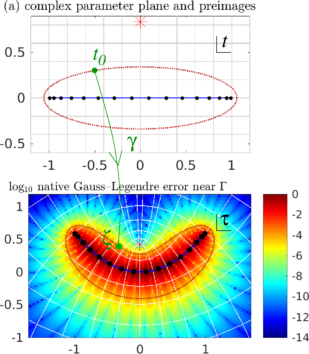
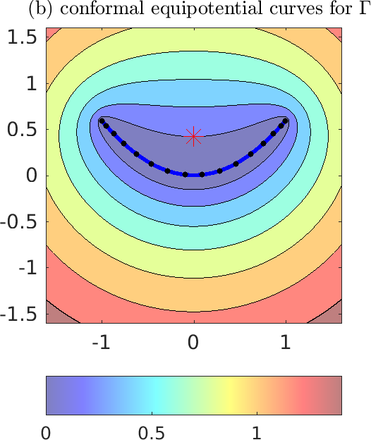
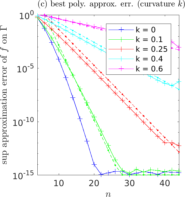
Figure 1: Native and complex-interpolatory evaluation errors for a simple parabolic panel $\Gamma$, for $I_{1}$ (complex double-layer) with density $\tilde{f}(t)=\sin(1+3t)$ as a function of parameter $t$. (a) $t$-plane preimage $[-1,1]$ (top plot) mapping to panel $\Gamma$ (bottom plot) via $\tau=\gamma(t)=t+ikt^{2}$ with curvature $k=0.6$, hence minimum radius of curvature $R=1/2k\approx 0.83$. Also shown are: $n=16$ Gauss–Legendre points and (bottom with colormap) their error in potential evaluation using the native (direct) scheme; an example target $\zeta$ and its preimage $t_{0}=\gamma^{-1}(\zeta)$ (large green dots); Bernstein ellipse for $t_{0}$ and its image (dotted red); Schwarz singularity $\tau_{\ast}=i/4k$ and its preimage $t_{\ast}=i/2k$ (red $\ast$’s); and Cartesian grid lines (grey) in the $t$-plane and their images (white). (b) Equipotential curves of $g(z)$ for the same panel $\Gamma$, showing “shielding” of the Schwarz singularity (red $\ast$) thus small $g\approx 0.2$ and $\rho\approx 1.22$. Contrast $\rho\approx 2.14$ for the Schwarz preimage in the $t$-plane. (c) Convergence in $n$ of polynomial approximation error of $f$ over $\Gamma$ (solid lines) for several curvatures $k$, compared to $C\rho^{-n}$ (dotted) predicted by section 2.3.

2.3 Effect of panel curvature on Helsing–Ojala convergence rate

The Helsing–Ojala method reviewed above is easy to implement, computationally cheap, and can achieve close to full numerical precision for target points very close to $\Gamma$. However, there is a severe loss of accuracy as $\Gamma$ becomes curved. This is striking in the central column of plots in fig. 2. This observation led Helsing–Ojala [24] and later users to recommend upsampling from a baseline $n=16$ to a larger $n$, such as $n=32$, even though the density and geometry were already accurately resolved at $n=16$. The “HO” $k=0.4$ plot in fig. 3 shows that even using $n=32$ has loss of accuracy near a moderately curved panel. This forces one to split panels beyond what is needed for the density representation, just to achieve good evaluation accuracy, increasing the cost.

The error in this method is essentially entirely due to the error of the polynomial approximation (19) of $f$ on $\Gamma$, because each monomial is integrated exactly (up to rounding error) as in Section 2.2.1. For this error there is a classical result that the best polynomial approximation converges geometrically in the degree, with rate controlled by the largest equipotential curve of $\Gamma$ in which $f$ is analytic. Namely, given the set $\Gamma$, let $g$ solve the potential problem in $\mathbb{R}^{2}$ (which we identify with $\mathbb{C}$),

$$\Delta g =0\qquad\mbox{ in }\mathbb{R}^{2}\backslash\Gamma$$

$$g =0\qquad\mbox{ on }\Gamma$$

$$g(\bm{x}) \sim\log|\bm{x}|\qquad\mbox{ as }|\bm{x}|\to\infty~{}.$$

For each $\rho>1$, define the level curve $C_{\rho}\mathrel{\mathop{\mathchar 58\relax}}=\{\tau\in\mathbb{C}\mathrel{\mathop{\mathchar 58\relax}}g(\tau)=\log\rho\}$. An example $g$ and its equipotential curves are shown in fig. 1(b); note that they are very different from the Bernstein ellipse images in the lower plot of fig. 1(a).

Theorem 3 (Walsh [50, §4.5]).

Let $\Gamma\subset\mathbb{C}$ be a set whose complement (including the point at infinity) is simply connected. Let $f\mathrel{\mathop{\mathchar 58\relax}}\Gamma\to\mathbb{C}$ extend analytically to a function analytic inside and on $C_{\rho}$, for some $\rho>1$. Then there is a sequence of polynomials $p_{n}(z)$ of degree $n=0,1,\ldots$ such that

$$|p_{n}(z)-f(z)|\;\leq\;C\rho^{-n}\qquad z\in\Gamma,\mbox{ for all }n=0,1,\ldots$$

where $C$ is a constant independent of $n$ and $z$.

To apply this to (19), we need to know the largest region in which $f$ may be continued as an analytic function, which is in general difficult. In practical settings the panels will have been refined enough so that on each panel preimage $\tilde{f}$ is interpolated in the parameter $t\in[-1,1]$ to high accuracy, thus we may assume that any singularities of $\tilde{f}$ are distant from $[-1,1]$. Yet, in moving from the $t$ to $\tau$ plane, the shape of the panel $\Gamma$ itself can introduce new singularities in $f$ which will turn out to explain well the observed loss of accuracy, as follows.

Proposition 4 (geometry-induced singularity in analytic continuation of density).

Let the pullback $\tilde{f}$ be a generic function analytic at $t_{\ast}$. Let $f(\tau)=\tilde{f}(t)$ where $\tau=\gamma(t)$. Let $t_{\ast}\in\mathbb{C}$ be such that $\gamma^{\prime}(t_{\ast})=0$ and $\gamma$ is analytic at $t_{\ast}$. Then generically $f(\tau)$ is not analytic at $\tau_{\ast}=\gamma(t_{\ast})$.

Proof.

Since the derivative vanishes, the Taylor expansion of the parameterization at $t_{\ast}$ takes the form $\gamma(t)=\tau_{\ast}+a_{2}(t-t_{\ast})^{2}+\dots$. If $f$ were analytic at $\tau_{\ast}$, expanding gives $f(\tau)=f_{0}+f_{1}(\tau-\tau_{\ast})+\dots$, then inserting $\tau=\gamma(t)$ gives $f_{0}+f_{1}a_{2}(t-t_{\ast})^{2}+\dots$ which must match, term by term, the Taylor expansion of the pullback $\tilde{f}(t)=\tilde{f}_{0}+\tilde{f}_{1}(t-t_{\ast})+\dots$. But generically $\tilde{f}_{1}\neq 0$, in which case there is a contradiction. ∎

Similar (more elaborate) arguments are known for singularities in the extension of Helmholtz solutions [33]. Here $\tau_{\ast}$ is an example of a singularity of the Schwarz function [14, 44] for the curve $\Gamma$. Recall that the Schwarz function $G$ is defined by $\overline{G(\tau)}=\gamma(\overline{\gamma^{-1}(\tau)})$, which is the analytic reflection of $\tau$ through the arc $\Gamma$. At points where $\gamma^{\prime}=0$, the inverse map $\gamma^{-1}$, hence the Schwarz function, has a square-root type branch singularity. Figure 1(a) shows that for a moderately bent parabolic panel, the Schwarz singularity is quite close to the concave side. Note that the above argument relies on $\tilde{f}$ having a generic expansion, which we believe is typical; we show below that its convergence rate prediction holds well in practice.

In summary, smooth but bent panels often have a nearby Schwarz singularity, which generically induces a singularity at this same location in the analytic continuation of the density $f$; then the equipotential for $\Gamma$ at this location controls the best rate of polynomial approximation, placing a fundamental limit on the Helsing–Ojala convergence rate in $n$. Figure 1(b) shows that, for a moderately bent panel, the close singularity is effectively shielded electrostatically by the concave panel, thus the convergence rate $\rho=e^{g(\tau)}$ is very small (close to 1). In fig. 1(c) we test this quantitatively: for a parabolic panel and simple analytic pullback density $\tilde{f}$ we compare the maximum error in $n$-term polynomial approximation on $\Gamma$ with the prediction from the above Schwarz–Walsh analysis. The agreement in rate is excellent over a range of curvatures. This also matches the loss of digits seen in the central column of figures 2 and 3: e.g. for even mild curvature $k=0.25$, $n=16$ achieves only 5 digits, and $n=32$ only 10 digits.

Conjecture 5 (Schwarz singularities at focal points).

Note that in the parabola example of fig. 1, a square-root type Schwarz singularity appears near $\Gamma$’s highest curvature point, at distance $R/2$ on the concave side, where $R$ is the radius of curvature. This is also approximately true for ellipses, whose foci induce singularities [44, §9.4]. We also always observe this numerically for other analytic curves. Hence we conjecture that it is a general result for analytic curves, in an approximate sense that becomes exact as $R\to 0$.

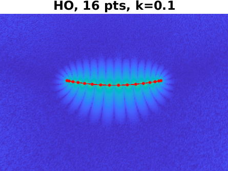
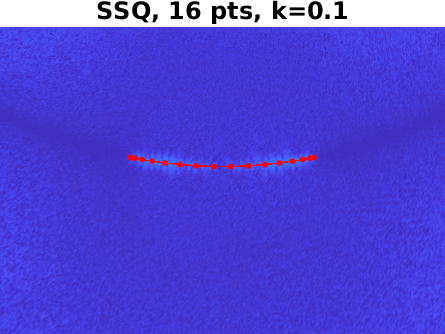
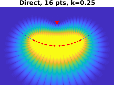
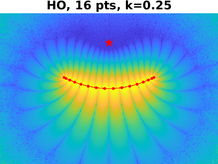
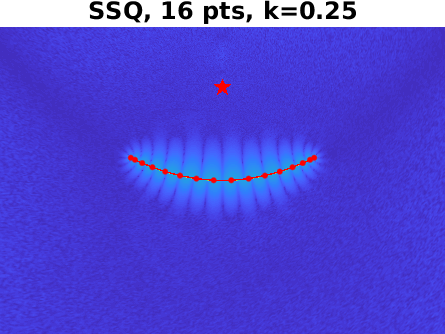
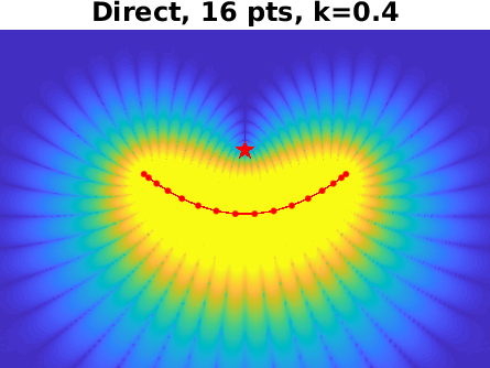
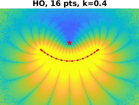
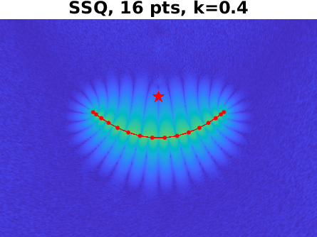
Figure 2: Spatial plot of relative errors in 2D quadratures for the Laplace double-layer (42) on $\Gamma$ a parabolic panel $\bm{g}(t)=(t,kt^{2})$, $-1\leq t\leq 1$, with smooth density $\rho(\bm{y})=y_{1}y_{2}$, using $n=16$ nodes. Each row shows a different curvature $k$. Left column: direct quadrature of section 2.1. Middle column: Helsing–Ojala (HO) quadrature of section 2.2. Right column: proposed singularity swap quadrature (SSQ) of section 2.4. The red $\ast$ is the Schwarz singularity of $\Gamma$.

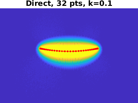
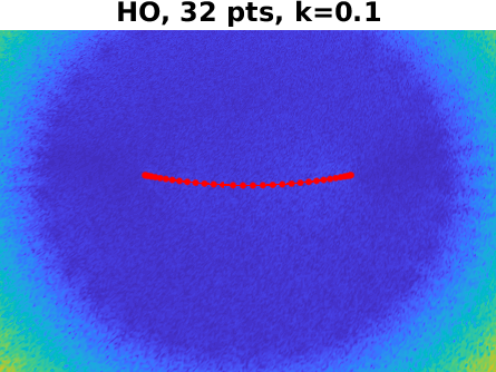
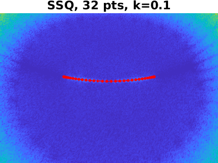
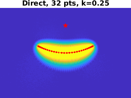
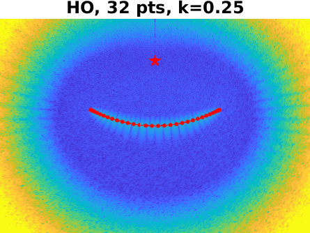
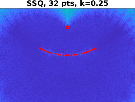
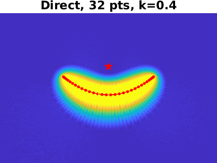
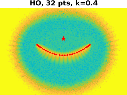
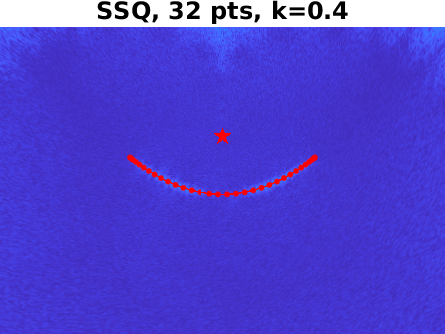
Figure 3: Same as fig. 2, after interpolating panel data to $n=32$ nodes.

2.4 Interpolatory quadrature using a real monomial basis

We now propose a “singularity swap” method which pushes the interpolation problem to the panel preimage $t\in[-1,1]$, thus bypassing the rather severe effects of curvature just explained. Recalling that the target point is $\zeta$, we first write the integrals (17) and (18) in parametric form

$$I_{L} =\int_{-1}^{1}h(t)\log Q(t)\,\operatorname{d\!}t~{},$$ (33)

$$I_{m} =\int_{-1}^{1}\frac{h(t)}{Q(t)^{m}}\operatorname{d\!}t~{},\quad m=1,2,\dots,$$ (34)

where we have introduced the displacement function $Q$ and the smooth function $h$,

$$Q(t) \mathrel{\mathop{\mathchar 58\relax}}=\gamma(t)-\zeta,$$ (35)

$$h(t) \mathrel{\mathop{\mathchar 58\relax}}=\tilde{f}(t)\mathinner{\!\left\lvert\gamma^{\prime}(t)\right\rvert}.$$ (36)

Now let $t_{0}$ be the root of $Q$ nearest to $[-1,1]$. (Unless the panel is very curved, there is only one such nearby root and it is simple.) Then $Q(t)/(t-t_{0})$ has a removable singularity at $t_{0}$, and hence it and its reciprocal are analytic in a larger neighborhood of $[-1,1]$ than the above integrands. By multiplying and dividing by $(t-t_{0})$,

$$I_{L} =\int_{-1}^{1}h(t)\log\frac{Q(t)}{t-t_{0}}\operatorname{d\!}t+\int_{-1}^{1}h(t)\log(t-t_{0})\operatorname{d\!}t~{},$$ (37)

$$I_{m} =\int_{-1}^{1}\frac{h(t)(t-t_{0})^{m}}{Q(t)^{m}}\frac{1}{(t-t_{0})^{m}}\operatorname{d\!}t~{},\quad m=1,2,\dots$$ (38)

which as we detail below can be handled as special cases of (17) and (18) for a new $\Gamma=[-1,1]$ written in the $t$ plane. We have “swapped” the singularity from the $\tau$ to the $t$ plane. As fig. 1 illustrates, the preimage of the Schwarz singularity has a much higher conformal distance from $[-1,1]$ than the actual singularity in the $\tau$-plane has from $\Gamma$, indicating much more rapid convergence.

Thus we now apply the Helsing–Ojala methods of section 2.2, but to $[-1,1]$ in the $t$ plane. Namely, as before, let $t_{j}$ and $w_{j}$, $j=1,\dots,n$ be the Gauss–Legendre quadrature for $[-1,1]$. The first integral in (37) is smooth, so direct quadrature is used. The second integral in (37) is evaluated via (21) and (29), setting $\Gamma=[-1,1]$, with the coefficients $c_{k}$ for the function $h(t)$ found by solving the Vandermonde system as in section 2.2. The first term $h(t)(t-t_{0})^{m}/Q(t)^{m}$ in (38) is smooth and plays the role of $f(\tau)$ in (18), so its coefficients are found similarly. (38) is then approximated by (22) with (25)–(28).

Remark 6.

Since in this scheme the new flat “panel” $[-1,1]$ is fixed, one may LU decompose the Vandermonde matrix once and for all, then use forward and back-substitution to solve for the coefficients $\{c_{k}\}$ given the $n$ samples of each of the two smooth functions, namely $\{h(t_{j})\}$ and $\{h(t_{j})(t_{j}-t_{0})^{m}/Q(t_{j})^{m}\}$, with only ${\mathcal{O}}(n^{2})$ effort.

Remark 7.

With a very curved panel it is possible that more than one root of $Q(t)$ is relevant; see fig. 4. In the case where poles $z_{1}$ and $z_{2}$ need to be cancelled, we have derived recursion formulae for $p_{k}^{m}(z_{1},z_{2})$ and $q_{k}(z_{1},z_{2})$ which generalize those in section 2.2.1. However, we have not found these to be needed in practice, so omit them.

2.4.1 Finding the roots of $Q(t)$

The only missing ingredient in the scheme just described is to find the nearest complex root $t_{0}$ satisfying

$$Q(t_{0})\mathrel{\mathop{\mathchar 58\relax}}=\gamma(t_{0})-\zeta=0~{},$$ (39)

i.e. the preimage of the (complex) target point $\zeta$ under the complexification of the panel map $\gamma$; see fig. 4. We base our method on that of [3] (where roots were needed only for the purposes of error estimation). Let $\operatorname{P}_{n}[\gamma](t)$ denote a degree $n-1$ polynomial approximant to $\gamma(t)$ on $[-1,1]$. Using the data at the Legendre nodes $\{t_{j}\}$, forming $\operatorname{P}_{n}[\gamma](t)$ is both well-conditioned and stable if we use a Legendre (or Chebyshev) expansion, and has an ${\mathcal{O}}(n^{2})$ cost. See [3] for details on how to use a Legendre expansion. Continuing each basis function to $\mathbb{C}$ gives a complex approximation

$$\tilde{Q}(t)\mathrel{\mathop{\mathchar 58\relax}}=\operatorname{P}_{n}[\gamma](t)-\zeta~{},$$ (40)

for which we seek roots nearest $[-1,1]$. Given a nearby starting guess, a single root of $\tilde{Q}$ can be found using Newton’s method, which converges rapidly and costs ${\mathcal{O}}(n)$ per iteration. A good starting guess is $t_{\mbox{\tiny init}}\approx s(\zeta)$, recalling that $s$ defined by (30) maps the panel endpoints to $\pm 1$. With this initialization, Newton iterations converge to the nearest root in most practical cases. The iterations can, however, be sensitive to the initial guess when two roots are both relatively close to $[-1,1]$, and sometimes converge to the second-nearest root. As illustrated in fig. 4, this typically happens only when the target point is on the concave side of a very curved panel.

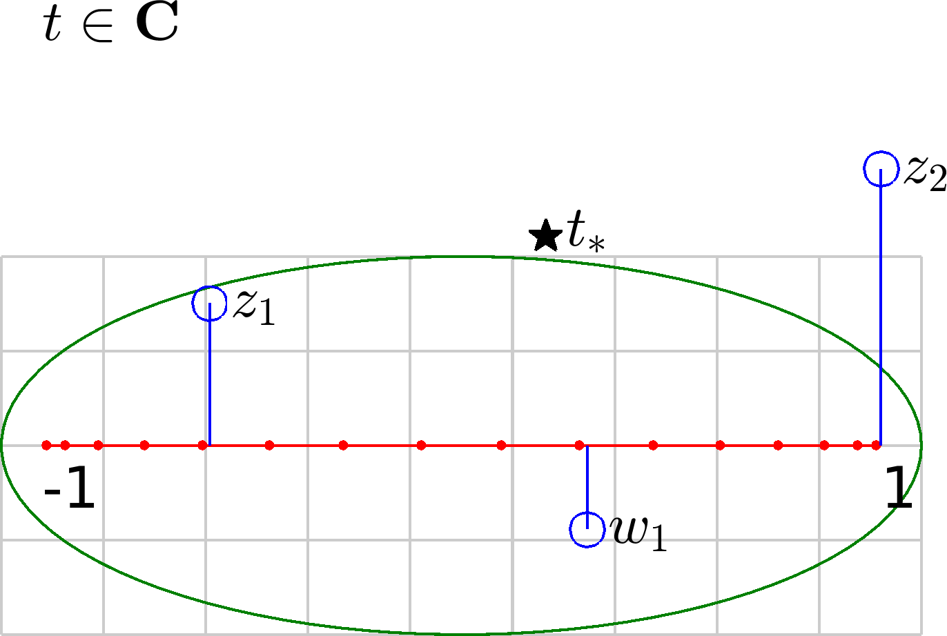
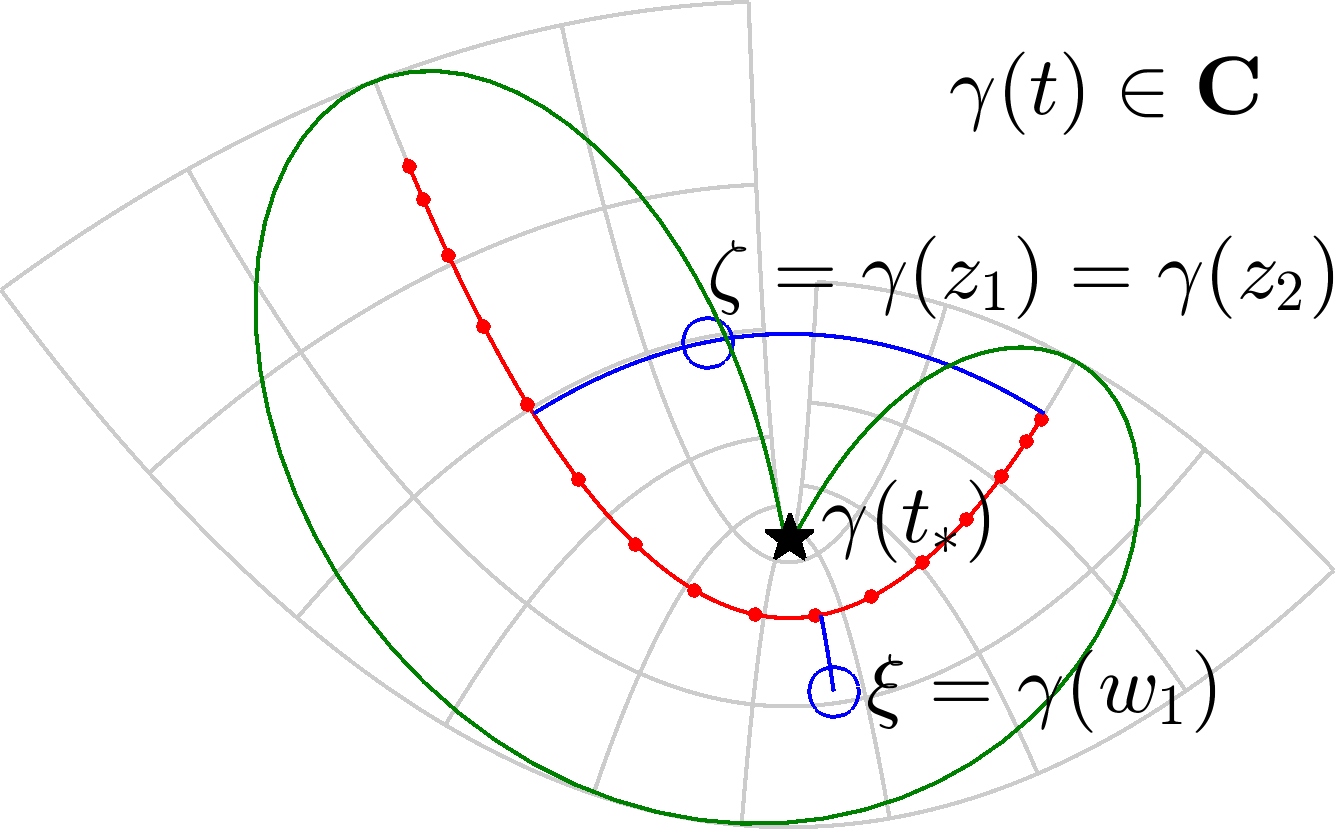
Figure 4: Illustration of the relationship between the roots of the displacement $Q(t)$, to the left, and target points in 2D physical space, to the right. The point $\xi$ corresponds to only one nearby root, $w_{1}$, while the point $\zeta$ corresponds to two nearby roots, $z_{1}$ and $z_{2}$. Note that only $z_{1}$ lies inside the Bernstein ellipse of radius ${\rho_{\epsilon}}$, marked green, such that it requires singularity swapping. The point $\gamma(t_{\ast})$ is the Schwarz singularity of the curve, marking the point where $\gamma^{-1}$ stops being single-valued.

A more robust, but also more expensive, way of finding the nearest root is to first find all $n-1$ roots of $\tilde{Q}$ at the same time, and then pick the nearest one. This can be done using a matrix-based method, which finds the roots as the eigenvalues to a generalized companion (or “comrade”) matrix [8]. This has a cost that is ${\mathcal{O}}(n^{3})$ if done naively, and ${\mathcal{O}}(n^{2})$ if done using methods that exploit the matrix structure [5].

In order to determine whether Newton iterations or a matrix-based method should be used for finding the root $t_{0}$, we suggest a criterion based on the distance to the nearest Schwarz singularity preimage of the panel, $t_{\ast}$, as this is a measure of the size of the region where $\gamma^{-1}$ is single-valued. Let ${\rho_{\epsilon}}$ be a Bernstein radius beyond which direct Gauss–Legendre quadrature is expected to have relative error $\epsilon$. E.g., ignoring the prefactor in (9) and solving for $\rho$,

$${\rho_{\epsilon}}\mathrel{\mathop{\mathchar 58\relax}}=\epsilon^{-1/2n}$$ (41)

is a useful estimate. Recalling (16), then $\rho(t_{\ast})\leq C{\rho_{\epsilon}}$, where we choose the constant $C=1.1$, indicates that there may be more than one nearby root, and that it is safer to use a matrix-based root finding method. For each panel, $t_{\ast}$ can be found at the time of discretization, by applying Newton’s method to the polynomial $\operatorname{P}_{n}[\gamma^{\prime}](t)=0$, with the initial guess $t_{\ast}\approx 0$.

Remark 8.

By switching to matrix-based root finding when there is a nearby Schwarz singularity, we get a root finding process that is robust also for very curved panels. However, in practical applications we have not observed it to be necessary, e.g. for the results of section 5. It is on the other hand necessary in the examples in figs. 2 and 3, because we there test the specialized quadrature at distances well beyond where it is required.

Remark 9.

The root finding process can be made efficient by computing the interpolants $\operatorname{P}_{n}[\gamma](t)$ and $\operatorname{P}_{n}[\gamma^{\prime}](t)$ for each segment at the time of discretization, such that they can be reused for every target point $\zeta$.

2.4.2 Tests of improved convergence rate for curved panels

We now compare the three methods: i) direct Gauss–Legendre quadrature, ii) Helsing–Ojala complex interpolatory quadrature, and iii) the proposed real singularity swap quadrature. We evaluate the Laplace double layer potential from a single panel,

$$u(\bm{x})=\int_{\Gamma}\rho(\bm{y})\frac{(\bm{y}-\bm{x})\cdot\bm{n}}{\mathinner{\!\left\lvert\bm{y}-\bm{x}\right\rvert}^{2}}\operatorname{d\!}s(\bm{y})~{}.$$ (42)

The panel is the same parabola as in fig. 1, i.e. $\bm{g}(t)=(t,kt^{2})$, or in complex form, $\gamma(t)=t+ikt^{2}$, and we explore the dependence on curvature $k$. In complex form, which is necessary to apply the quadratures, the layer potential is (see appendix A)

$$u(\zeta)=-\operatorname{Im}\int_{-1}^{1}\frac{\rho(\gamma(t))\gamma^{\prime}(t)\operatorname{d\!}t}{\gamma(t)-\zeta}~{}.$$ (43)

Figs. 2 and 3 compare the three schemes for various curvatures, for $n=16$ and $n=32$ respectively. For $n=32$ all data is upsampled by Lagrange interpolation from $n=16$ (which is already adequate to represent it to machine precision). The error is in all cases measured against a reference solution computed using adaptive quadrature (integral in MATLAB with abstol and reltol set to eps), and the relative error $E_{\text{rel}}$ computed against the maximum value of $u$ on the grid. To see how they behave when pushed to their limits, we deliberately apply the quadratures much further away than necessary, i.e. also in the region where direct quadrature achieves full numerical accuracy.

The direct errors (left column of each figure) have magnitudes controlled by the images of Bernstein ellipses under the parameterization, as explained in section 2.1. The Helsing–Ojala scheme (middle column) is much improved over direct quadrature, but, because of its convergence rates dependence (section 2.3) the reduction in accuracy is severe as curvature increases, although it can to some can extent be ameliorated by using $n=32$. In addition, there is an error in the quadrature that grows with the distance from the panel, particularly for $n=32$, due to amplification of roundoff error in the upward recurrence for the integrals $\{p_{1},\dots,p_{n}\}$. This was also noted in [24], where the suggested fix was to instead run the recurrence backwards for distant points, starting from a value of $p_{n}$ computed using the direct quadrature. This avoids the problem of catastrophic accuracy loss, but only because specialized quadrature is used where direct quadrature would be sufficient. The bottom middle plot of fig. 3 shows at best 10 accurate digits, and that only over quite a narrow range of distances, making the design of algorithms to give a uniform accuracy for all target locations rather brittle.

For the proposed singularity swap quadrature (right columns), the there is still a loss of accuracy with increased curvature, but the improvement over Helsing–Ojala is striking. The instability of upwards recurrence is also much more mild.

Remark 10.

The loss of accuracy with increased curvature can for the singularity swap quadrature be explained by considering the roots of the displacement function $Q(t)$. We have “swapped” out the nearest root $t_{0}$, so the region of analyticity of the regularized integrand $h(t)(t-t_{0})/Q(t)$ is bounded by the second nearest root of $Q(t)$, illustrated by $z_{2}$ in fig. 4. This limits the convergence rate of the polynomial coefficients $\left\{c_{k}\right\}$, such that we may need to upsample the panel in order for the coefficients to fully decay. In the case of our parabolic panel, the second nearest root gets closer with increased curvature, which explains why upsampling to 32 points is necessary to achieve full accuracy in some locations. Note that for the upsampling to be beneficial, the coefficients for $k>n$ must be nonzero. This is only the case if the components of the integrand ($\rho$, $\gamma$, $\gamma^{\prime}$) are upsampled separately, before the integrand is evaluated at the new nodes.

3 Line integrals on curved panels in three dimensions

Since the logarithmic kernel is irrelevant in 3D, we care about the parametric form of (1),

$$I_{m}=I_{m}(\bm{x})=\int_{-1}^{1}\frac{\tilde{f}(t)}{\mathinner{\!\left\lvert\bm{g}(t)-\bm{x}\right\rvert}^{m}}\mathinner{\!\left\lvert\bm{g}^{\prime}(t)\right\rvert}\operatorname{d\!}t,\qquad m=1,3,5,\dots,$$ (44)

where $\Gamma=\bm{g}([-1,1])$ is an open curve in $\mathbb{R}^{3}$, and $\tilde{f}$ incorporates the density and possibly other smooth denominator factors in the kernel $K$. Fixing the target $\bm{x}$, then introducing the 3D squared distance function $R^{2}$ (analogous to (10)) and the smooth function $h$,

$$R(t)^{2} \mathrel{\mathop{\mathchar 58\relax}}=\mathinner{\!\left\lvert\bm{g}(t)-\bm{x}\right\rvert}^{2}=\left(g_{1}(t)-x_{1}\right)^{2}+\left(g_{2}(t)-x_{2}\right)^{2}+\left(g_{3}(t)-x_{3}\right)^{2},$$ (45)

$$h(t) \mathrel{\mathop{\mathchar 58\relax}}=\tilde{f}(t)\mathinner{\!\left\lvert\bm{g}^{\prime}(t)\right\rvert}~{},$$ (46)

we can write (44) as

$$I_{m}=\int_{-1}^{1}\frac{h(t)}{\left(R(t)^{2}\right)^{m/2}}\operatorname{d\!}t.$$ (47)

This integrand has singularities at the roots of $R(t)^{2}$, which, since the function is real for real $t$, come in complex conjugate pairs $\{t_{0},\overline{t_{0}}\}$. How to find these roots is discussed shortly in section 3.2; for now we assume that they are known. As in 2D, if the line is not very curved, and the target is nearby, there is only one nearby pair of roots.

We construct a quadrature for (47) as in the 2D case (38), except that now there is a conjugate pair of near singularities to cancel. Thus we write (47) as

$$I_{m}\;=\;\int_{-1}^{1}H(t)\cdot\frac{1}{\left((t-t_{0})(\overline{t-t_{0}})\right)^{m/2}}\operatorname{d\!}t~{},\qquad\mbox{where }H(t)\mathrel{\mathop{\mathchar 58\relax}}=\frac{h(t)\left((t-t_{0})(\overline{t-t_{0}})\right)^{m/2}}{\left(R(t)^{2}\right)^{m/2}}~{}.$$ (48)

$H(t)$ can be expected to be analytic in a much larger neighborhood of $[-1,1]$ than the integrand. As in section 2.4, we now represent $H(t)$ in a real monomial basis,

$$H(t)=\sum_{k=1}^{n}c_{k}t^{k-1}~{},$$ (49)

getting the coefficients $c_{k}$ by solving the Vandermonde system

$$A\bm{c}=\bm{h}$$

with the matrix entries $A_{ij}=t_{i}^{j-1}$, where, as before, $\{t_{i}\}_{i=1}^{n}$ are the panel’s parameter Legendre nodes in $[-1,1]$. We fill $\bm{h}$ by evaluating its entries $\{H(t_{i})\}_{i=1}^{n}$. By analogy with (24), we set

$$P_{k}^{m}(t_{0})=\int_{-1}^{1}\frac{t^{k-1}}{\left((t-t_{0})(\overline{t-t_{0}})\right)^{m/2}}\operatorname{d\!}t\;=\;\int_{-1}^{1}\frac{t^{k-1}}{|t-t_{0}|^{m}}\operatorname{d\!}t~{},\qquad k=1,\dots,n~{},$$ (50)

which one can evaluate to machine accuracy using recurrence relations as described in the next section. Combining (50) and (49) gives the final quadrature approximation to (44),

$$I_{m}\approx\sum_{k=1}^{n}c_{k}P_{k}^{m}(t_{0})~{}.$$ (51)

The adjoint method of section 2.2.2 can again be used to solve for a weight vector $\bm{\lambda}^{m}$ whose inner product with $\bm{h}$ approximates $I_{m}$. As in section 2.4, the error in (51) is essentially due to the convergence rate of the best polynomial representation (49) on $[-1,1]$, which is likely to be rapid because of the absence of curvature effects (section 2.3).

3.1 Recurrence relations for 3D kernels on a straight line

The above singularity swap has transformed the integral on a curved line $\Gamma$ in 3D to (48), whose denominator corresponds to that of a straight line in 3D. Such upward recursions are available in [46, App. B], where they were used for Stokes quadratures near straight segments. We will here present them with some improvements which increase their stability for $t_{0}$ in certain regions of $\mathbb{C}$. We present the case of a single root pair $\{t_{0},\overline{t_{0}}\}=t_{r}\pm it_{i}$, for orders $m=1,3,5$, noting that, while we have derived formulae for double root pairs, we have found that they are never needed in practice. To simplify notation (matching notation for $I_{n}^{\beta}$ in [46, App. B]), we write

$$b \mathrel{\mathop{\mathchar 58\relax}}=-2t_{r}, c \mathrel{\mathop{\mathchar 58\relax}}=t_{r}^{2}+t_{i}^{2}, d \mathrel{\mathop{\mathchar 58\relax}}=t_{i}^{2},$$ (52)

and for the distances to the parameter endpoints we write

$$u_{1} =\sqrt{(1+t_{r})^{2}+t_{i}^{2}}=|1+t_{0}|, u_{2} =\sqrt{(1-t_{r})^{2}+t_{i}^{2}}=|1-t_{0}|.$$ (53)

Beginning with $m=1$ and $k=1$, the integral (50) is

$$P_{1}^{1}(t_{0})=\int_{-1}^{1}\frac{\operatorname{d\!}t}{\sqrt{(t-t_{r})^{2}+t_{i}^{2}}}=\log\left(1-t_{r}+u_{2}\right)-\log\left(-1-t_{r}+u_{1}\right).$$ (54)

This expression suffers from cancellation for $t_{0}$ close to $[-1,1]$, and must be carefully evaluated. To begin with, it is more accurate in the left half plane, even though the integral is symmetric in $t_{r}$, so the accuracy can be increased by evaluating it after the substitution $t_{r}\to-|t_{r}|$. In addition, the argument of the second logarithm of (54) suffers from cancellation when $|t_{r}|<1$ and $t_{i}^{2}\ll(1-|t_{r}|)^{2}$, even after the substitution. In this case we evaluate it using a Taylor series in $t_{i}$,

$$-(1-|t_{r}|)+\sqrt{(1-|t_{r}|)^{2}+t_{i}^{2}} =(1-|t_{r}|)\sum_{n=1}^{\infty}\frac{(-1)^{n}(2n)!}{(1-2n)(n!)^{2}(4^{n})}\left(\frac{t_{i}}{1-|t_{r}|}\right)^{2n}=\mathrel{\mathop{\mathchar 58\relax}}S_{1}(t_{0}).$$ (55)

We achieve sufficient accuracy by applying this series evaluation to points inside the rhombus described by $4|t_{i}|<1-|t_{r}|$, evaluating the series to $n=11$. For $k>1$ the upward recursions of [46] are stable, such that

$$P_{1}^{1}(t_{0}) =\log(1+|t_{r}|+\sqrt{(1+|t_{r}|)^{2}+t_{i}^{2}})$$ (56)

$$\quad-\begin{cases}\log S_{1}(t_{0}),&\text{if}\quad 4|t_{i}|<1-|t_{r}|,\\ \log(-1+|t_{r}|+\sqrt{(-1+|t_{r}|)^{2}+t_{i}^{2}}),&\text{otherwise},\end{cases}$$ (57)

$$P_{2}^{1}(t_{0}) =u_{2}-u_{1}-\frac{b}{2}P_{1}^{1}(t_{0}),$$ (58)

$$P_{k+1}^{1}(t_{0}) =\frac{1}{k}\left(u_{2}-(-1)^{n-1}u_{1}+\frac{(1-2k)b}{2}P_{k}^{1}(t_{0})-(k-1)cP_{k-1}^{1}(t_{0})\right).$$ (59)

For $m=3$, the formula from [46] for $k=1$ contains a conditional statement for points on the real axis ($d=0$), where the pair of two conjugate roots $\left\{t_{0},\overline{t_{0}}\right\}$ merge into a double root. In finite precision, this property causes a region around the real axis where the formula is inaccurate, namely two cones extending outwards from the endpoints $\pm 1$. To get high accuracy there, we consider the integral with shifted limits,

$$P_{1}^{3}(t_{0})=\int_{-1-t_{r}}^{1-t_{r}}\left(s^{2}+t_{i}^{2}\right)^{-3/2}\operatorname{d\!}s=\left[S_{3}(s)\right]_{-1-t_{r}}^{1-t_{r}}~{},$$ (60)

where the antiderivative $S_{3}$ is evaluated by forming a Maclaurin series of the integrand in $t_{i}$, and then integrating that series exactly in $s$, thus

$$S_{3}(s)=\int\left(s^{2}+t_{i}^{2}\right)^{-3/2}\operatorname{d\!}s\;=\;\frac{\mathinner{\!\left\lvert s\right\rvert}}{s^{3}}\sum_{n=0}^{\infty}\left(-\frac{1}{4}\right)^{n+1}\!\!\frac{(2n+2)!}{((n+1)!)^{2}}\left(\frac{t_{i}}{s}\right)^{2n}.$$ (61)

We find that we get sufficiently high accuracy in the region of interest by truncating this series to 30 terms, denoted by $\tilde{S}_{3}(s)$, and finally evaluating the integrals for $m=3$ as

$$P_{1}^{3}(t_{0}) =\begin{cases}\tilde{S}_{3}(1-t_{r})-\tilde{S}_{3}(-1-t_{r}),&\text{if}\quad 0<\frac{\mathinner{\!\left\lvert t_{i}\right\rvert}}{\mathinner{\!\left\lvert t_{r}\right\rvert}-1}<0.6,\\ \frac{1}{2d}\left(\frac{b+2}{u_{2}}-\frac{b-2}{u_{1}}\right),&\text{otherwise},\end{cases}$$ (62)

$$P_{2}^{3}(t_{0}) =\frac{1}{u_{1}}-\frac{1}{u_{2}}-\frac{b}{2}P_{1}^{3}(t_{0}),$$ (63)

$$P_{k+1}^{3}(t_{0}) =P_{k-1}^{1}(t_{0})-bP_{k}^{3}(t_{0})-cP_{k-1}^{3}(t_{0}).$$ (64)

The series evaluation can be optimized by defining a succession of narrower cones, using fewer terms in each cone.

For $m=5$ and $k=1$ we need to repeat the process of finding a power series that we can use in cones around the real axis, extending from the endpoints. We now consider

$$P_{1}^{5}(t_{0})=\int_{-1-t_{r}}^{1-t_{r}}\left(s^{2}+t_{i}^{2}\right)^{-5/2}\operatorname{d\!}s,$$ (65)

and the antiderivative of the Maclaurin series of the integrand is

$$S_{5}(s)=\int\left(s^{2}+t_{i}^{2}\right)^{-5/2}\operatorname{d\!}s\;=\;\frac{\mathinner{\!\left\lvert s\right\rvert}}{s^{5}}\sum_{n=0}^{\infty}\frac{(-1)^{n+1}\left(4n^{2}+8n+3\right)}{3(n+2)2^{2n+1}}\frac{(2n)!}{(n!)^{2}}\left(\frac{t_{i}}{s}\right)^{2n}.$$ (66)

Truncating this series to a maximum of 50 terms, denoted by $\tilde{S}_{5}(s)$, we now evaluate the integrals for $m=5$ as

$$P_{1}^{5}(t_{0}) =\begin{cases}\tilde{S}_{5}(1-t_{r})-\tilde{S}_{5}(-1-t_{r}),&\text{if}\quad 0<\frac{\mathinner{\!\left\lvert t_{i}\right\rvert}}{\mathinner{\!\left\lvert t_{r}\right\rvert}-1}<0.7,\\ \frac{1}{3d}\left(\frac{b+2}{2u_{2}^{3}}-\frac{b-2}{2u_{1}^{3}}+2P_{1}^{3}(t_{0})\right),&\text{otherwise},\end{cases}$$ (67)

$$P_{2}^{5}(t_{0}) =\frac{1}{3u_{1}^{3}}-\frac{1}{3u_{2}^{3}}-\frac{b}{2}P_{1}^{5}(t_{0}),$$ (68)

$$P_{k+1}^{5}(t_{0}) =P_{k-1}^{3}(t_{0})-bP_{k}^{5}(t_{0})-cP_{k-1}^{5}(t_{0}).$$ (69)

Note that our expression for $P_{2}^{5}$ is different from the one found in [46]; ours avoids a conditional.

3.2 Finding the roots of $R(t)^{2}$

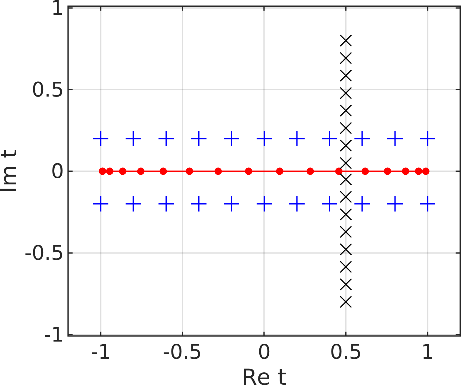
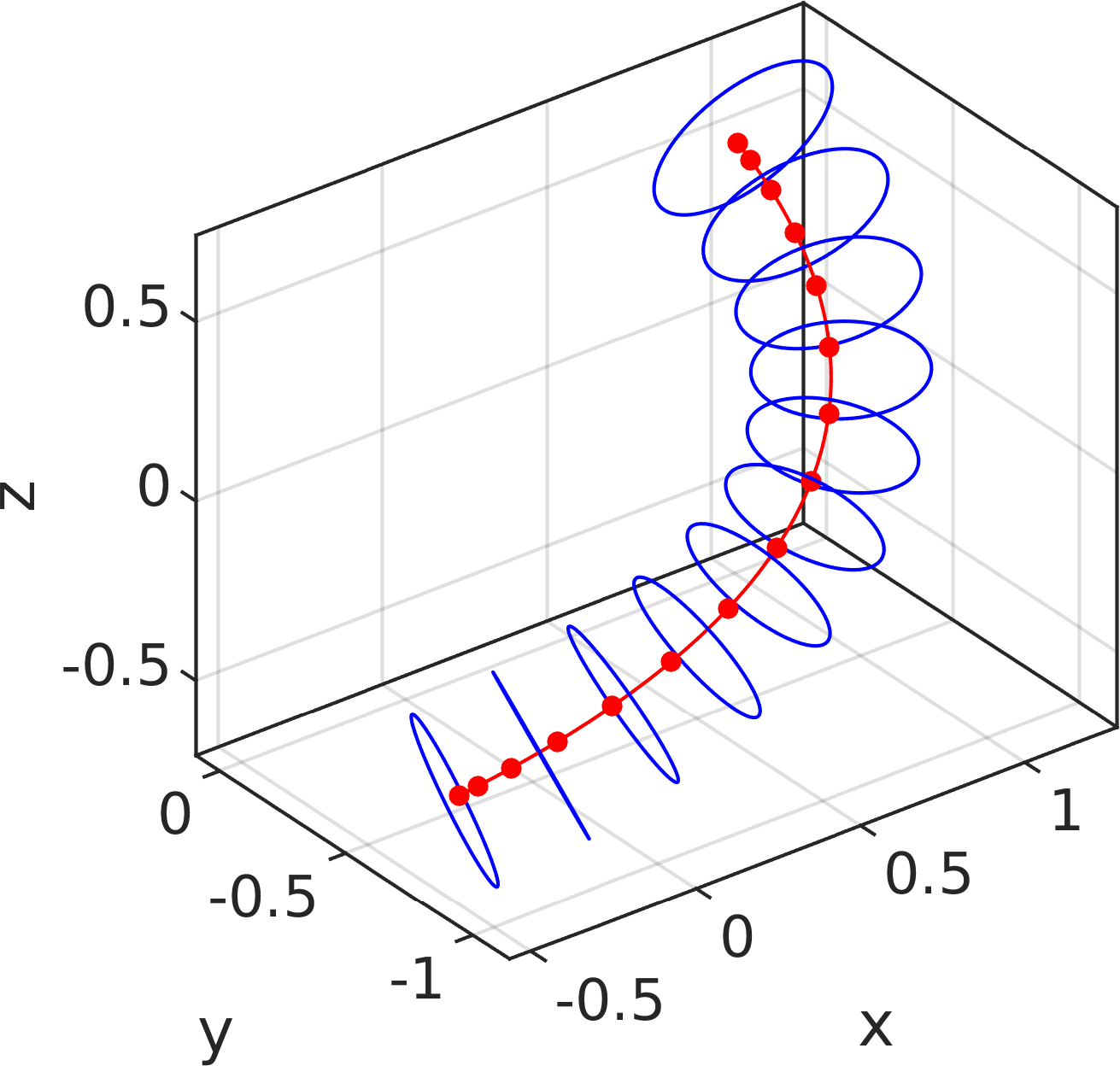
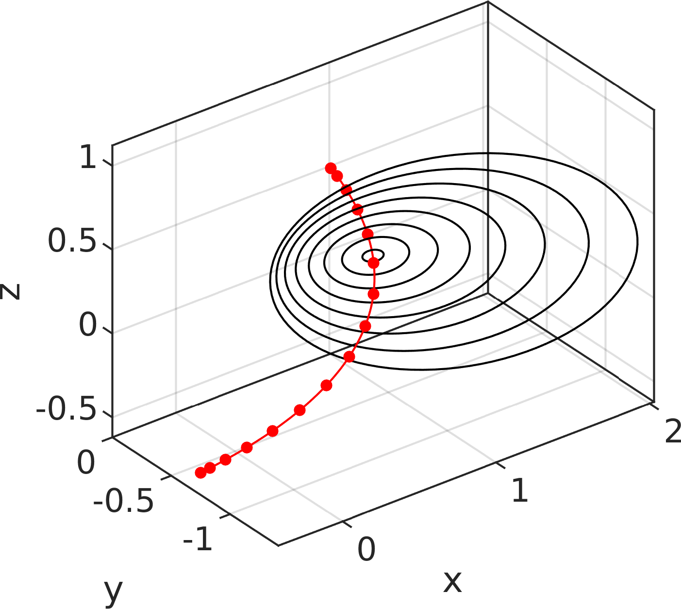
Figure 5: Correspondence between complex roots of the 3D squared distance function $R(t)^{2}$ in (45) and target points in $\mathbb{R}^{3}$, close to a curve. The red dots (left) are the Legendre nodes on $[-1,1]$, mapped to a curve in space (center & right). The roots marked with a blue + in the left figure correspond to the blue circles in the middle figure, while the roots marked with a black x in the left figure correspond to the black circles in the right figure.

In three dimensions, the nearby roots of the squared distance function (45) do not correspond to a single point in space, as was the case in 2D (see fig. 4). Instead, each complex conjugate pair of roots $\{t_{0},\overline{t_{0}}\}$ near $[-1,1]$ corresponds to a circle in space looped around $\Gamma$. To see this, let $\bm{g}_{r}$ and $\bm{g}_{i}$ be the real and imaginary parts of the complexification of the parametrization,

$$\bm{g}(t)=\bm{g}_{r}(t)+i\bm{g}_{i}(t).$$ (70)

Then, the roots of (45) satisfy

$$R(t)^{2}=\mathinner{\!\left\lvert\bm{g}_{r}(t)-\bm{x}\right\rvert}+2i\bm{g}_{i}(t)\cdot\left(\bm{g}_{r}(t)-\bm{x}\right)-\mathinner{\!\left\lvert\bm{g}_{i}(t)\right\rvert}^{2}=0.$$ (71)

For this to hold in both real and imaginary components for a given $t$, the point $\bm{x}$ must satisfy

$$\left\{\begin{array}[l]{rcl}\bm{g}_{i}(t)\cdot(\bm{g}_{r}(t)-\bm{x})&=&0,\\ \mathinner{\!\left\lvert\bm{g}_{r}(t)-\bm{x}\right\rvert}&=&\mathinner{\!\left\lvert\bm{g}_{i}(t)\right\rvert}^{2}.\end{array}\right.$$ (74)

The above equations describe the intersection of a plane with a sphere, and are satisfied by the circle of radius $\mathinner{\!\left\lvert\bm{g}_{i}(t)\right\rvert}$ that is centered at $\bm{g}_{r}(t)$, and lies in the plane normal to $\bm{g}_{i}(t)$. All points in $\mathbb{R}^{3}$ corresponding to the root $t$ lie on this circle. For an illustration of this, see fig. 5.

In order to construct a quadrature for a given target point $\bm{x}$, we need to find the roots $t$ to (45), which are the points satisfying the complex equation

$$R(t)^{2}=\left(g_{1}(t)-x_{1}\right)^{2}+\left(g_{2}(t)-x_{2}\right)^{2}+\left(g_{3}(t)-x_{3}\right)^{2}=0.$$ (75)

We form a polynomial approximation $\operatorname{P}_{n}[\bm{g}](t)$ of $\bm{g}(t)$ using the existing real Gauss–Legendre nodes $\{\bm{g}(t_{j})\}$. We then need to find the roots of the polynomial

$$\tilde{R}(t)^{2}\mathrel{\mathop{\mathchar 58\relax}}=\left(\operatorname{P}_{n}[g_{1}](t)-x_{1}\right)^{2}+\left(\operatorname{P}_{n}[g_{2}](t)-x_{2}\right)^{2}+\left(\operatorname{P}_{n}[g_{3}](t)-x_{3}\right)^{2}.$$ (76)

These can be found using either of the root-finding methods discussed in section 2.4.1. We here limit ourselves to finding the root pair $\{t_{0},\overline{t_{0}}\}$ closest to $[-1,1]$, using Newton’s method. We find that a stable initial guess can be obtained using a linear mapping in the plane containing $\bm{x}$ and the two closest discretization points on $\Gamma$, which we denote by $\bm{g}_{j}\mathrel{\mathop{\mathchar 58\relax}}=\bm{g}(t_{j})$ and $\bm{g}_{k}\mathrel{\mathop{\mathchar 58\relax}}=\bm{g}(t_{k})$. The initial guess $t_{\mbox{\tiny init}}$ is then set to one of the two points satisfying

$$\frac{\operatorname{Re}t_{\mbox{\tiny init}}-t_{j}}{t_{k}-t_{j}}=\frac{\left(\bm{x}-\bm{g}_{j}\right)\cdot\left(\bm{g}_{k}-\bm{g}_{j}\right)}{\mathinner{\!\left\lvert\bm{g}_{k}-\bm{g}_{j}\right\rvert}^{2}},\qquad\mbox{ and }\quad\frac{\mathinner{\!\left\lvert t_{\mbox{\tiny init}}-t_{j}\right\rvert}}{\mathinner{\!\left\lvert t_{k}-t_{j}\right\rvert}}=\frac{\mathinner{\!\left\lvert\bm{x}-\bm{g}_{j}\right\rvert}}{\mathinner{\!\left\lvert\bm{g}_{k}-\bm{g}_{j}\right\rvert}}.$$ (77)

This is the exact root for the case of $\Gamma$ a straight line.

Compared to the 2D case, we find that the accuracy of our method in 3D is more sensitive to the implementation details of the root-finding algorithm, especially for roots very close to the interval $[-1,1]$. Below are a number of noteworthy observations:

• The convergence of Newton’s method will deteriorate for roots that are close to the real axis (or on it, when $|\operatorname{Re}t_{0}|>1$). This is because the root $t_{0}$ and its conjugate $\overline{t_{0}}$ will merge into a double root at $\operatorname{Im}t_{0}=0$, which reduces Newton’s method to linear convergence. In finite precision, we find that this hampers the convergence of Newton’s method also for roots that lie close the real axis. To ameliorate this problem, we let our root-finding routine switch to Muller’s method [41] if Newton has not converged within a certain number of iterations (we use 20). In our tests, this appears to be a stable root-finding process for all points requiring special quadrature, such that we can apply direct quadrature to points where neither Newton’s nor Muller’s methods converge. For additional robustness, one could also switch to the comrade matrix method in such cases.

• Just as in the 2D case, once the root $t_{0}$ is known we can determine if special quadrature is needed using the Bernstein radius $\rho(t_{0})$ criterion at the end of section 2.4.1.

• We find that it is important for accuracy to find the roots using the approximation (76) of $R^{2}$. If instead $R^{2}$ is approximated as $\operatorname{P}_{n}[R^{2}](t)$, then 1–2 digits of accuracy are lost close to $[-1,1]$. If roots are computed from this form, for example if the comrade matrix method is used, then they can be polished by taking one or two Newton steps of (76), thereby recovering the lost accuracy.

• For panels discretized with more than $n=16$ points, we find that the best accuracy is achieved if the roots are found using Legendre expansions truncated to 16 terms. In general, our recommendation is to not use an underlying discretization with $n$ larger than 16, and then upsample to more points when evaluating the SSQ, if necessary (see 10).

4 Summary of algorithm

Below is a step by step summary of our algorithm for evaluating the potential generated by a single open curve panel $\Gamma$, in 2D or 3D, discretized using $n$ Gauss–Legendre points. Specifically, we describe how to get the weight vector $\bm{\lambda}$ as defined in section 2.2.2, from which one of the line integrals (17), (18) or (44) can be approximated by $I=\bm{\lambda}^{T}\bm{f}$ for any sample vector $\bm{f}$ of densities (or density times smooth geometric factors). Recall that potentials are defined by such line integrals, possibly in the 2D case via complexification as shown in Appendix A. (We omit the optional finding of the panel’s Schwarz singularity, and use of the robust comrade-matrix method given in section 2.4.1, since we find that it is not needed in practice.)

There is an overall algorithm option (flag) which may take the values “no upsampling”, “upsampling” or “upsampling with upsampled direct”. Either variety of upsampling is more expensive, but can increase accuracy; the latter avoids some special weight computations so is the cheaper of the two.

Precomputations for panel $\Gamma$:

1. Choose a suitable polynomial basis (e.g. Legendre or Chebyshev; we use the former). The analytic continuation of the chosen basis functions must be simple to evaluate (as is the case for Legendre). Form the degree $n-1$ polynomial approximation of the panel parameterization $\operatorname{P}_{n}[\bm{g}](t)$ in this basis; this can be done by solving a $n\times n$ linear system with right-hand side the coordinates of the nodes $\bm{y}_{j}=\bm{g}(t_{j})$, $j=1,\dots,n$.

2. Given the desired tolerance $\epsilon$, set the critical Bernstein radius $\rho_{\epsilon}$ via (41).

For each given target point $\bm{x}$:

1. Use a cheap criterion to check if $\bm{x}$ is a candidate for near evaluation, based on the minimum distance between the target point and the panel nodes:

   $$\bm{x}\text{ candidate if }\min_{\bm{y}_{i}\in\Gamma}\mathinner{\!\left\lvert\bm{y}_{i}-\bm{x}\right\rvert}<D,$$ (78)

   where $D$ is a multiple of the panel length $h$ (at $n=16$ we use $D=h$ for full accuracy). If not a candidate, use the direct rule (6) then exit; more specifically the weights are

   $$\lambda_{j}=w_{j}|\bm{g}^{\prime}(t_{j})|K(\bm{x},\bm{y}_{j})~{},\qquad j=1,\ldots,n.$$ (79)

2. Find the complex target preimage $t_{0}$ from the basis approximation to $\bm{g}(t)$: In 2D, use Newton’s method applied to (40) to find the root $t_{0}$. In 3D, use Newton (complemented by Muller’s method) applied to (76) to find the root pair $\{t_{0},\overline{t_{0}}\}$.

3. If $\rho(t_{0})\geq{\rho_{\epsilon}}$, use the direct rule (79) and exit. If no upsampling, set $\tilde{n}=n$, or if upsampling, $\tilde{n}=2n$. If “upsampling with upsampled direct”, check if $\sqrt{{\rho_{\epsilon}}}\leq\rho(z)<{\rho_{\epsilon}}$, and if so use the degree $n-1$ approximants to resample the kernel and density to the $m$ new nodes and use the upsampled $m$-node version of the direct formula (79), then exit.

4. We now do special quadrature for evaluation at $\bm{x}$. More precisely, we use the singularity swap method with parameter target $t_{0}$ and panel $[-1,1]$, as follows.

   For 2D, compute the monomial integral vector $\bm{p}$, being $\{p_{k}^{m}(t_{0})\}_{k=0}^{\tilde{n}}$, or for the logarithmic case $\{q_{k}(t_{0})\}_{k=0}^{\tilde{n}}$, via the recurrences (25)–(29) applied to $[-1,1]$. For 3D, it is $\{P_{k}^{m}(t_{0})\}_{k=0}^{\tilde{n}}$, computed via the various recurrences of section 3.1.

5. Solve the adjoint Vandermonde system (32) where the $\tilde{n}$-by-$\tilde{n}$ matrix $A$ involves the nodes on $[-1,1]$, and the right-hand side is the $\bm{p}$ just computed. We find that the Björck-Pereyra algorithm [10] is even faster than using a precomputed LU decomposition of $A$.

6. Finally, one must apply corrections to turn $\bm{\lambda}$ into a set of weights that act on the samples of $f$, rather than the singularity-swapped smooth functions involving $h(t)$ or $H(t)$. First multiply each weight $\lambda_{j}$ by the Jacobian factor $|\bm{g}^{\prime}(t_{j})|$, according to (36) or (46). Then:

   • For the log case in 2D, according to (37), add $w_{j}\log(Q(t_{j})/(t_{j}-t_{0}))$ to each weight $\lambda_{j}$.

   • For the power-law case in 2D, according to (38), multiply each weight by $((t_{j}-t_{0})/Q(t_{j}))^{m}$.

   • In 3D, according to (48), multiply each weight by $\bigl{(}(t_{j}-t_{0})(\overline{t_{j}-t_{0}})/R(t_{j})^{2}\bigr{)}^{m/2}$.

5 Numerical tests

In section 2 we already performed basic comparisons of prior methods and the proposed singularity swap quadrature in the 2D case. Now we give results of more extensive 2D tests and the 3D case.

The 2D and 3D quadrature methods of this paper have been implemented in a set of Matlab routines. These are available online [1], together with the programs used for all the numerical experiments reported here. The computationally intensive steps of the 3D quadrature have been implemented in C, with basic OpenMP parallelization, and interfaced to Matlab using MEX. This allows very rapid computation of quadrature weights: on the computer used for the numerical results of this section, which is a 3.6 GHz quad-core Intel i7-7700, we can find the roots (preimages) of $4.7\times 10^{6}$ target points per second, and compute $3.2\times 10^{6}$ sets of target-specific quadrature weights per second, for $n=16$ (without upsampling).

5.1 Evaluating a layer potential in two dimensions

To study quadrature performance when evaluating an actual layer potential, we solve a simple test problem using an integral equation method, then evaluate the solution using either the Helsing–Ojala method or our proposed method. Following [24] we test the Laplace equation $\Delta u=0$ in the interior of the starfish-shaped domain $\Omega$ given by $\gamma(t)=(1+0.3\cos(5t))e^{it}$, $t\in[0,2\pi)$, and we choose Dirichlet boundary conditions $u=u_{e}$ on ${\partial\Omega}$ with data $u_{e}(\zeta)=\log\mathinner{\!\left\lvert 3+3i-\zeta\right\rvert}$. We have picked this data to be very smooth, since the errors then are due to quadrature, rather than density resolution, making it easier to compare methods.

We discretize ${\partial\Omega}$ using composite Gauss–Legendre quadrature, with $n=16$ points per panel. The panels are formed using the following adaptive scheme. The interval $[0,2\pi)$ is recursively bisected into segments that map to panels, until all panels satisfy a resolution condition, and all pairs of neighboring segments differ in length by a ratio this is no more than 2 (i.e. level-restriction). The resolution condition is based on the Legendre expansion coefficients $\{\hat{\gamma}^{\prime}_{k}\}$ of the panel derivative $\gamma^{\prime}(t)$: a panel is deemed resolved to a tolerance $\epsilon$ if $\max(\mathinner{\!\left\lvert\hat{\gamma}^{\prime}_{n-1}\right\rvert},\mathinner{\!\left\lvert\hat{\gamma}^{\prime}_{n}\right\rvert})<\epsilon\mathinner{\!\left\lVert\bm{\hat{\gamma}}^{\prime}\right\rVert}_{\infty}$. While somewhat ad-hoc, this produces a solution with a relative error that is comparable to $\epsilon$, for a smooth problem (see figs. 6 and 7).

The solution to the Laplace equation is represented using the double layer potential (43), which results in a second kind integral equation in $\rho$. This is solved using the Nyström method and the above discretization, which is straightforward due to the layer potential being smooth on ${\partial\Omega}$. For further details on this solution procedure, see, for example, [20] or [24]. Once we have $\rho$, we evaluate the layer potential using quadrature at sets of points in $\Omega$, and compute the error by comparing with the exact solution, $u_{e}$. We compare two methods:

1. The Helsing–Ojala (HO) method summarized in section 2.2.

2. The proposed singularity swap quadrature (SSQ), as outlined in section 4.

In both methods we test “no upsampling” with $n=16$, and “upsampling with upsampled direct” with $\tilde{n}=32$.

In our first test, shown in fig. 6, we solve the problem using a quite coarse discretization (adaptive with $\epsilon=10^{-6}$), choose ${\rho_{\epsilon}}=1.8$ (corresponding via (41) to a more conservative error of $10^{-8}$), and evaluate the solution on a $300\times 300$ uniform grid covering the domain. Far from the boundary the solution shows around the expected 6 digit accuracy. Notice that, since only eight panels are used, they are highly curved. HO gets only 2 digits at $\tilde{n}=16$ and scarcely more at $\tilde{n}=32$, whereas SSQ gets 3 digits at $\tilde{n}=16$ and the “full” 6 digits at $\tilde{n}=32$. This shows that upsampled SSQ achieves the full expected accuracy using the efficient discretization chosen for this accuracy, whereas HO would require further panel subdivision beyond that needed to achieve the requested Nyström accuracy.

As a second test, we solve the same problem, this time using a fine discretization (adaptive with $\epsilon=10^{-14}$), and pick ${\rho_{\epsilon}}=3$, corresponding via (41) to around $\epsilon\approx 10^{-15}$ at $n=16$. The result is 32 panels (similar to the 35 panels used in [24]). First we evaluate the solution on a uniform $250\times 250$ grid covering all of $\Omega$. Then we evaluate the solution on the slice of $\Omega$ defined by the mapping $\gamma(t)$ of the square in $\mathbb{C}$ defined by $\operatorname{Re}t\in[1.66\pi,1.76\pi]$ and $\operatorname{Im}t\in[d_{\text{min}},0.15]$. Here we use two grids in $t$: one uniform $250\times 250$ with $d_{\text{min}}=10^{-3}$, and one $250\times 250$ that is uniform in $\operatorname{Re}t$ and logarithmic in $\operatorname{Im}t$, with $d_{\text{min}}=10^{-8}$. Here we only show the results when using upsampling, since both methods require that to achieve maximum accuracy (without upsampling, HO gets 8 digits and SSQ 9 digits). The results of this test are shown in 7. Both schemes are able to achieve high accuracy here: both get 13 digits close to the boundary, and both drop to 11-12 digits when tested extremely close to the boundary. However, contrary to the previous test, the proposed SSQ does lose around 1 digit relative to HO, in the distance range $10^{-3}$ to $10^{-8}$. We do not have an explanation for this loss.

To summarize this experiment, SSQ is much better than HO for panels that are resolved to lower accuracies, because these panels may be quite curved. When panels are resolved to close to machine precision the methods are about the same, with HO attaining a slightly smaller error.

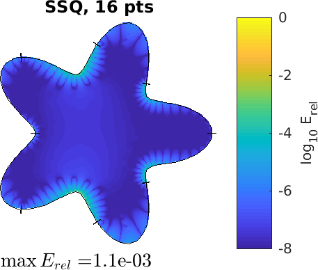
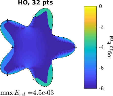
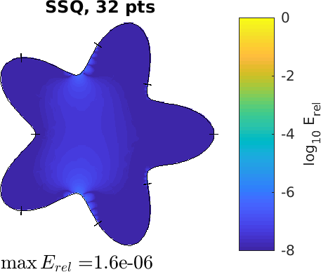
Figure 6: Comparison of 2D quadratures when evaluating Laplace double layer potential using a coarse discretization (adaptive with $\epsilon=10^{-6}$, giving 8 panels). Left column: Helsing–Ojala (HO). Right column: proposed singularity swap quadrature (SSQ). Top row: no upsampling. Bottom row: upsampling.

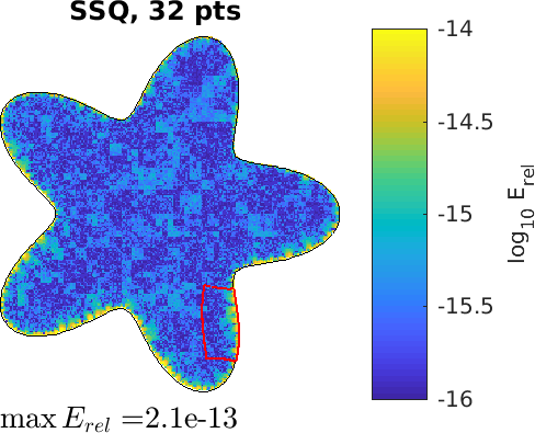
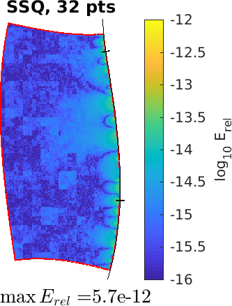
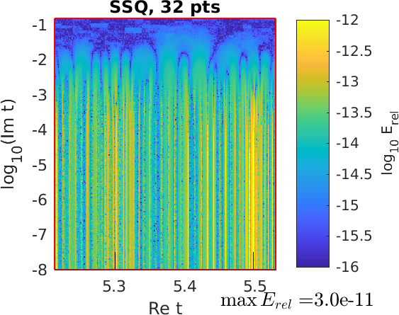
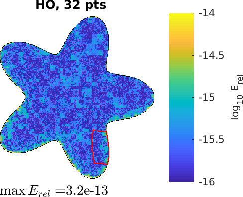
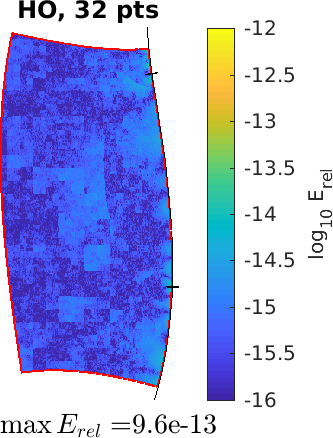
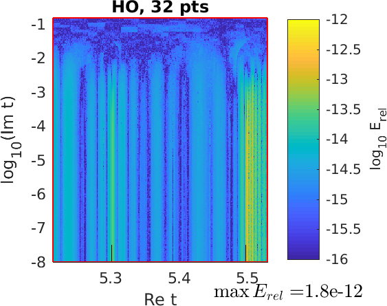
Figure 7: Comparison of 2D quadratures when evaluating Laplace double layer potential using a high-accuracy discretization (adaptive with $\epsilon=10^{-14}$, giving 32 panels) and upsampling. Top row: proposed singularity swap quadrature (SSQ). Bottom row: Helsing–Ojala (HO). Near region (center) is marked red in the left plots. Right plot shows error versus root location in near region, with exponential grading of the imaginary part, proportional to distance. Note the different color scale used in the near region.

5.2 Evaluating the field due to a slender body in three dimensions

To test our method in 3D, we evaluate the slender body approximation of Stokes flow around a thin filament. In this approximation, the flow due to a fiber with centerline $\Gamma$ and radius $\varepsilon\ll 1$ is given by the line integral (see e.g. [34])

$$\bm{u}(\bm{x})=\int_{\Gamma}\left({\mathcal{S}}(\bm{x}-\bm{y})+\frac{\varepsilon^{2}}{2}{\mathcal{D}}(\bm{x}-\bm{y})\right)\bm{f}(\bm{y})\operatorname{d\!}s(\bm{y}).$$ (80)

Here $\bm{f}$ is given force data, defined on the centerline, ${\mathcal{S}}$ is the Stokeslet kernel, defined as

$${\mathcal{S}}(\bm{R})=\frac{\bm{I}}{|\bm{R}|}+\frac{\bm{R}\bm{R}^{T}}{|\bm{R}|^{3}},$$ (81)

and ${\mathcal{D}}$ is the doublet kernel, defined as

$${\mathcal{D}}(\bm{R})=\frac{1}{2}\Delta{\mathcal{S}}(\bm{R})=\frac{\bm{I}}{|\bm{R}|^{3}}-3\frac{\bm{R}\bm{R}^{T}}{|\bm{R}|^{5}}.$$ (82)

Note that ${\mathcal{S}}$ and ${\mathcal{D}}$ are tensors, and $\bm{I}$ is the $3\times 3$ identity. To apply our quadrature, we first write (80) in kernel-split form,

$$\bm{u}(\bm{x}) =I_{1}+I_{3}+I_{5},$$ (83)

where

$$I_{1} =\int_{\Gamma}\frac{\bm{f}(\bm{y})}{{|\bm{R}|}}\operatorname{d\!}s(\bm{y}),$$ (84)

$$I_{3} =\int_{\Gamma}\frac{\left(\bm{R}\bm{R}^{T}+\varepsilon^{2}\bm{I}/2\right)\bm{f}(\bm{y})}{{|\bm{R}|^{3}}}\operatorname{d\!}s(\bm{y}),$$ (85)

$$I_{5} =-\frac{3\varepsilon^{2}}{2}\int_{\Gamma}\frac{\bm{R}\bm{R}^{T}\bm{f}(\bm{y})}{{|\bm{R}|^{5}}}\operatorname{d\!}s(\bm{y}),$$ (86)

and $\bm{R}\mathrel{\mathop{\mathchar 58\relax}}=\bm{x}-\bm{y}$. Once in this form, one can compute modified weights for $I_{1}$, $I_{3}$, and $I_{5}$ using the proposed SSQ quadrature.

For our tests, we use the force data $\bm{f}(\bm{y})=\bm{y}$ and $\varepsilon=10^{-3}$. We let $\Gamma$ be the closed curve shown in fig. 8, which is described by a Fourier series with decaying random coefficients,

$$\bm{\gamma}(t) =\operatorname{Re}\sum_{k=-20}^{20}\frac{\bm{c}(k)}{5+|k|}\hat{\bm{\gamma}}(k)e^{2\pi ikt},\quad t\in[0,1),$$ (87)

where the components of $\bm{c}(k)$ are complex and normally distributed random numbers. We subdivide $\Gamma$ into panels by recursively bisecting the curve until each panel is resolved to a tolerance $\epsilon$, using a criterion similar to that used in section 5.1: A panel is deemed resolved if the expansion coefficients $\{\hat{s}_{k}\}$ of the speed function $s(t)=\mathinner{\!\left\lvert\bm{\gamma}^{\prime}(t)\right\rvert}$ satisfy $\max(\mathinner{\!\left\lvert\hat{s}_{n-1}\right\rvert},\mathinner{\!\left\lvert\hat{s}_{n}\right\rvert})<\epsilon\mathinner{\!\left\lVert\bm{\hat{s}}\right\rVert}_{\infty}$. Each panel is then discretized using $n=16$ Gauss–Legendre nodes.

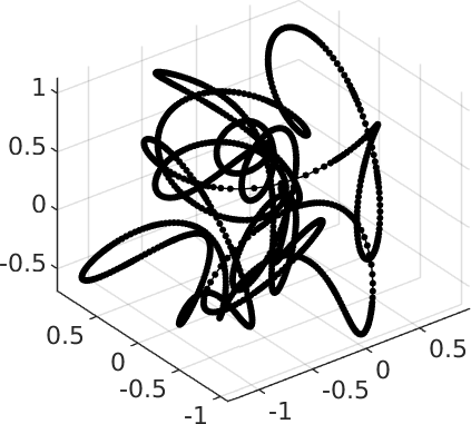
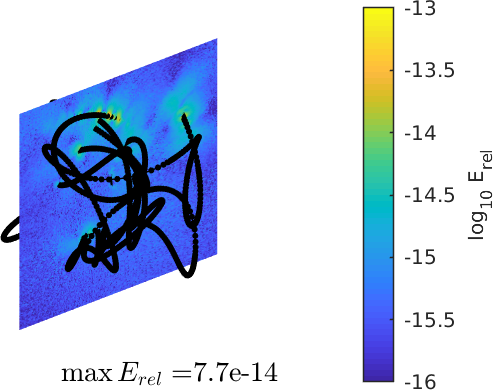
Figure 8: Left: The curve in 3D described by (87), showing the discretization nodes (for $\epsilon=10^{-10}$) as dots. Right: Relative error when evaluating the slender body field (80) on the shown slice using the proposed SSQ method.

5.2.1 Comparison to adaptive quadrature

As a comparison for our method, and also to compute reference values, we have implemented a scheme for nearly singular 3D line quadrature based on per-target adaptive refinement: For a given target point $\bm{x}$, nearby panels are recursively subdivided until each panel $\Gamma_{i}$ satisfies $\min_{\bm{y}\in\Gamma_{i}}|\bm{x}-\bm{y}|<h_{i}$, where $h_{i}$ is the arc length of $\Gamma_{i}$. Each newly formed panel is discretized using $n=16$ Gauss–Legendre points, and the required data $(\bm{\gamma},|\bm{\gamma}^{\prime}|,\bm{f})$ is interpolated to these points from the parent panel using barycentric Lagrange interpolation [9]. After this new set of panels is formed, the field (80) can be accurately evaluated at $\bm{x}$ using the Gauss–Legendre quadrature weights, since all source panels then are far away from $\bm{x}$, relative to their own length. This scheme is relatively simple to implement, but has the drawback of requiring an increasingly large amount of interpolations and kernel evaluations as $\bm{x}$ approaches $\Gamma$.

In an attempt to obtain a fair comparison of runtimes between the adaptive quadrature and the proposed SSQ, we will only report on the time spent in codes that are of similar efficiency, in terms of implementation. For the adaptive quadrature, we will therefore report the time spent on interpolations (reported as $t_{\text{interp}}$), since those are implemented using a combination of C and BLAS, and omit the time spent on the recursive subdivisions, since that is presently implemented in a relatively slow prototype code. For the SSQ, we will report on the total time spent on finding roots and computing the new quadrature weights (reported $t_{\text{weights}}$), since all the expensive steps of that algorithm have been implemented in C. For both methods we will also report on the time spent on near evaluations of the Stokeslet and doublet kernels (reported as $t_{\text{eval}}$), since those are computed using the same code. Far field evaluation times are omitted, since they are identical. Thus $t_{\text{eval}}+t_{\text{interp}}$ is somewhat less than the total time for an adaptive scheme, whereas $t_{\text{eval}}+t_{\text{weights}}$ is the total time for our proposed SSQ.

5.2.2 Results

As a first test, we evaluate the $\bm{u}(\bm{x})$ velocity field (80) on $200\times 200$ points covering the $xz$-slice $[-1.4,1.4]\times 0.25\times[-1.4,1.4]$. The curve is adaptively discretized using $\epsilon=10^{-10}$, which results in 187 panels. For each point-panel interaction, we evaluate the SSQ using data upsampled to 32 Gauss–Legendre points, for all target points within the Bernstein radius ${\rho_{\epsilon}}=3$. Unlike the 2D case, we find that this upsampling is necessary for achieving accurate results. The error is measured against a reference computed using the adaptive quadrature and a discretization with 18-point panels, created using $\epsilon=5\cdot 10^{-14}$ (this is to ensure that the grids are different, and that the reference grid is better resolved). The resulting error field, shown in 8, indicates that the SSQ can recover at least 13 digits of accuracy at all the target points. However, the largest errors are at the points closest to the curve.

To further compare the behavior close to the curve, we compute $\bm{u}$ at a set of random target points all located at the same distance $d$ away from $\Gamma$. The test setup and results are listed in table 1. As expected, the computational costs (kernel evaluations and runtime) of the proposed SSQ quadrature does not vary with the distance between the target points and the curve, as long as the target points are within the near evaluation threshold. The adaptive quadrature, on the other hand, has costs that grow slowly as the distance decreases, since more and more source points are required to evaluate the integral. The SSQ also appears to be a factor of several times cheaper, both in number of evaluations ($4$ to $7$ times less) and in runtime ($2.5$ to $5$ times faster), even though our timings are under-estimates for adaptive quadrature. However, the error for the SSQ in this application starts to grow for close distances: for instance, at $d=10^{-4}$ the table shows that it loses around 2 digits relative to the $\epsilon$ at which the panels were discretized.

Remark 11.

This loss of accuracy in this application for targets at small distance $d$ is not entirely surprising. The SSQ method gives weights $\bm{\lambda}$ at the given nodes for integrating the kernels $|\bm{R}|^{-1}$, $|\bm{R}|^{-3}$, and $|\bm{R}|^{-5}$. The resulting integrals diverge, respectively as $\log d$, $d^{-2}$, and $d^{-4}$. We have checked that, for these kernels with generic densities, the relative errors of SSQ are close to machine precision (around 13 digits), even though as $d\to 0$ the $\lambda_{j}$ are growing and oscillatory. However, the Stokes kernels (84)–(86) involve near-vanishing numerator factors (such as $\bm{R}\bm{R}^{T}$) which partially cancel the singularities, leading to much smaller values for the integrals. In our method such factors are incorporated into a modified density $\tilde{f}$ in (44), thus catastrophic cancellation as $d\to 0$ is inevitable for this application (this is also true for the straight fiber method of [46]). This could only be avoided by a more specialized set of recursions for the full Stokes kernels (85) and (86).

Parameters		Adaptive quad.				Singularity swap quad. (SSQ)
$d$	$\epsilon$	$N_{\text{eval}}$	$t_{\text{eval}}$	$t_{\text{interp}}$	$\max E_{\text{rel}}$	$N_{\text{eval}}$	$t_{\text{eval}}$	$t_{\text{weights}}$	$\max E_{\text{rel}}$
1.0e-02	1.0e-10	2.8e+06	0.17 s	0.45 s	7.3e-14	6.3e+05	0.06 s	0.19 s	1.7e-13
1.0e-02	1.0e-06	4.7e+06	0.30 s	0.78 s	4.8e-09	1.3e+06	0.12 s	0.14 s	4.8e-09
1.0e-04	1.0e-10	4.4e+06	0.26 s	0.55 s	5.9e-11	6.3e+05	0.06 s	0.18 s	2.0e-08
1.0e-04	1.0e-06	6.3e+06	0.38 s	0.86 s	5.5e-08	1.3e+06	0.12 s	0.13 s	7.7e-05

Table 1: Adaptive vs proposed SSQ quadratures for 3D Stokes slender body. There are 5000 random target points located distance $d$ from the curve $\Gamma$, which is discretized using tolerance $\epsilon$. For either method, the number of near-field kernel evaluations is $N_{\text{eval}}$ and the time spent on them $t_{\text{eval}}$. $t_{\text{interp}}$ is the time interpolating to temporary grids in the adaptive quadrature. $t_{\text{weights}}$ is the total time finding the interpolatory quadrature weights in the proposed SSQ (rootfinding, recursions and Vandermonde solve). Error is measured against a reference solution.

6 Conclusions

We have presented an improved version of the monomial approximation method of Helsing and Ojala [24, 19, 37] for nearby evaluation of 2D layer potentials discretized with panels. At the cost of a single Newton search for the target preimage, our method uses singularity cancellation to “swap” the singular problem on the general curved (complex) panel for one on the standard (real) panel $[-1,1]$, much improving the error. Hence we call the method “singularity swap quadrature” (SSQ). We emphasize that it is not the conditioning of the monomial interpolation problem that improves—the Vandermonde matrix is exponentially ill-conditioned in either case—rather, the exponential convergence rate improves markedly in the case of curved panels. In the case of a Nyström discretization adapted to a requested tolerance, this allows SSQ to achieve this tolerance when HO would demand further subdivision. We gave a quantitative explanation for both the HO and SSQ convergence rates using classical polynomial approximation theory: the HO rate is limited by electrostatic “shielding” of a nearby Schwarz singularity by the panel itself.

We then showed that the singularity swap idea gives a close-evaluation quadrature for line integrals on general curves in 3D, which has so far been missing from the literature. The (to these authors) delightful fact that complex analysis can help in a 3D application relies on analytically continuing the squared-distance function (45). Note that QBX [7, 30] cannot apply to line integrals in 3D, since the potential becomes singular (in the transverse directions) approaching the curve. We demonstrated 3D SSQ in a slender body theory Stokes application. We found that, at least when targets are only moderately close, comparable accuracies to a standard adaptive quadrature are achieved with several times fewer kernel evaluations, and, in a simple C implementation, speeds several times faster.

As 11 discusses, in the Stokes application, in order to retain full relative accuracy at arbitrarily small target distances a new set of recurrences for these particular kernels would be essential; we leave this for future work. Of course, the slender body approximation breaks down for distances comparable to or smaller than the body radius, so that the need for full accuracy at such small distances is debatable.

Appendix A 2D kernels in complex variable form

In order to use either the Helsing–Ojala quadrature or the two-dimensional singularity swap quadrature proposed in this paper, the complex variable form of the kernel is required. In [42, App. A]) the single and double layer kernels for several common 2D elliptic PDEs are listed. If analytically separated into a kernel-split form [20, Sec. 6], these kernels can be summarized as having singularities of the following types. (Note that this is a subset of the forms derived in [22, Sec. 6], which include denominators up to $|\bm{y}-\bm{x}|^{6}$.)

$$\int\rho\frac{(\bm{y}-\bm{x})\cdot\bm{f}}{\mathinner{\!\left\lvert\bm{y}-\bm{x}\right\rvert}^{2}}\operatorname{d\!}s(\bm{y}), \int\rho\log\mathinner{\!\left\lvert\bm{y}-\bm{x}\right\rvert}\operatorname{d\!}s(\bm{y}),$$ (88)

$$\int\rho\frac{(\bm{y}-\bm{x})}{\mathinner{\!\left\lvert\bm{y}-\bm{x}\right\rvert}^{2}}\operatorname{d\!}s(\bm{y}), \int\frac{\bm{f}\cdot(\bm{y}-\bm{x})(\bm{y}-\bm{x})(\bm{y}-\bm{x})\cdot\bm{\hat{n}}}{\mathinner{\!\left\lvert\bm{y}-\bm{x}\right\rvert}^{4}}\operatorname{d\!}s(\bm{y}).$$ (89)

Let us use the following identifications between vectors in $\mathbb{R}^{2}$ and points in $\mathbb{C}$: $\bm{x}=z$, $\bm{y}=\tau$, $\bm{\hat{n}}=\nu$, $\gamma(t)=\bm{g}(t)$, and $\bm{f}={\mathfrak{f}}$. Our rewrites use the following definitions and basic results:

$$\bm{x}\cdot\bm{y} =\operatorname{Re}\left[z\bar{\tau}\right],$$ (90)

$$\nu =i\gamma^{\prime}/\mathinner{\!\left\lvert\gamma^{\prime}\right\rvert},$$ (91)

$$\operatorname{d\!}s(\bm{y}) =i\bar{\nu}\operatorname{d\!}\tau=-i\nu\operatorname{d\!}\bar{\tau}.$$ (92)

Throughout, $\rho$ and $\bm{f}$ are assumed to be arbitrary functions that are smooth and real-valued. The above integrals can then in complex form be written as

$$\int\rho\frac{(\bm{y}-\bm{x})\cdot\bm{f}}{\mathinner{\!\left\lvert\bm{y}-\bm{x}\right\rvert}^{2}}\operatorname{d\!}s(\bm{y}) =-\operatorname{Im}\int\frac{\rho{\mathfrak{f}}\bar{\nu}\operatorname{d\!}\tau}{\tau-z},$$ (93)

$$\int\rho\frac{(\bm{y}-\bm{x})}{\mathinner{\!\left\lvert\bm{y}-\bm{x}\right\rvert}^{2}}\operatorname{d\!}s(\bm{y}) =\overline{\int\frac{\rho\bar{\nu}}{(\tau-z)}i\operatorname{d\!}\tau},$$ (94)

$$\int\rho\log\mathinner{\!\left\lvert\bm{y}-\bm{x}\right\rvert}\operatorname{d\!}s(\bm{y}) =-\operatorname{Im}\int\rho\bar{\nu}\log(\tau-z)\operatorname{d\!}\tau,$$ (95)

$$\int\frac{\bm{f}\cdot(\bm{y}-\bm{x})(\bm{y}-\bm{x})(\bm{y}-\bm{x})\cdot\bm{\hat{n}}}{\mathinner{\!\left\lvert\bm{y}-\bm{x}\right\rvert}^{4}}\operatorname{d\!}s(\bm{y}) =\frac{1}{4i}\left[\overline{\int\frac{(\bar{\tau}-\bar{z}){\mathfrak{f}}\operatorname{d\!}\tau}{(\tau-z)^{2}}}+\overline{\int\frac{(\bar{{\mathfrak{f}}}+{\mathfrak{f}}\bar{\nu}^{2})\operatorname{d\!}\tau}{\tau-z}}-\int\frac{{\mathfrak{f}}\operatorname{d\!}\tau}{\tau-z}\right].$$ (96)

As an example of how these can be used, if we let $\bm{f}=\bm{\hat{n}}$ in (93) and use that $\nu\bar{\nu}=1$, we directly get the complex form of the double layer kernel of the Laplace equation,

$$\int\rho\frac{(\bm{y}-\bm{x})\cdot\bm{n}}{\mathinner{\!\left\lvert\bm{y}-\bm{x}\right\rvert}^{2}}\operatorname{d\!}s(\bm{y})=-\operatorname{Im}\int\frac{\rho\operatorname{d\!}\tau}{\tau-z}.$$ (97)

References

- af Klinteberg [2019] L. af Klinteberg. Line quadrature library (linequad), 2019. URL http://github.com/ludvigak/linequad.
- af Klinteberg and Tornberg [2017] L. af Klinteberg and A.-K. Tornberg. Error estimation for quadrature by expansion in layer potential evaluation. Adv. Comput. Math., 43(1):195–234, 2017. doi:10.1007/s10444-016-9484-x.
- af Klinteberg and Tornberg [2018] L. af Klinteberg and A.-K. Tornberg. Adaptive Quadrature by Expansion for Layer Potential Evaluation in Two Dimensions. SIAM J. Sci. Comput., 40(3):A1225–A1249, 2018. doi:10.1137/17M1121615.
- Atkinson [1997] K. Atkinson. The numerical solution of integral equations of the second kind. Cambridge University Press, 1997.
- Aurentz et al. [2014] J. L. Aurentz, R. Vandebril, and D. S. Watkins. Fast computation of eigenvalues of companion, comrade, and related matrices. BIT Numer. Math., 54(1):7–30, 2014. doi:10.1007/s10543-013-0449-x.
- Barnett et al. [2015] A. Barnett, B. Wu, and S. Veerapaneni. Spectrally Accurate Quadratures for Evaluation of Layer Potentials Close to the Boundary for the 2D Stokes and Laplace Equations. SIAM J. Sci. Comput., 37(4):B519–B542, 2015. doi:10.1137/140990826.
- Barnett [2014] A. H. Barnett. Evaluation of Layer Potentials Close to the Boundary for Laplace and Helmholtz Problems on Analytic Planar Domains. SIAM J. Sci. Comput., 36(2):A427–A451, 2014. doi:10.1137/120900253.
- Barnett [1975] S. Barnett. A companion matrix analogue for orthogonal polynomials. Linear Algebra Appl., 12(3):197–202, 1975. doi:10.1016/0024-3795(75)90041-5.
- Berrut and Trefethen [2004] J.-P. Berrut and L. N. Trefethen. Barycentric Lagrange Interpolation. SIAM Rev., 46(3):501–517, 2004. doi:10.1137/S0036144502417715.
- Björck and Pereyra [1970] A. Björck and V. Pereyra. Solution of Vandermonde Systems of Equations. Math. Comput., 24(112):893, 1970. doi:10.2307/2004623.
- Bruno and Haslam [2007] O. P. Bruno and M. C. Haslam. Regularity theory and superalgebraic solvers for wire antenna problems. SIAM J. Sci. Comput., 29(4):1375–1402, 2007.
- Carvalho et al. [2018] C. Carvalho, S. Khatri, and A. D. Kim. Asymptotic analysis for close evaluation of layer potentials. J. Comput. Phys., 355:327–341, 2018.
- Cortez [2018] R. Cortez. Regularized Stokeslet segments. J. Comput. Phys., 375:783–796, 2018. doi:10.1016/j.jcp.2018.08.055.
- Davis [1974] P. J. Davis. The Schwarz function and its applications. The Mathematical Association of America, Buffalo, N. Y., 1974. The Carus Mathematical Monographs, No. 17.
- Donaldson and Elliott [1972] J. D. Donaldson and D. Elliott. A Unified Approach to Quadrature Rules with Asymptotic Estimates of Their Remainders. SIAM J. Numer. Anal., 9(4):573–602, 1972. doi:10.1137/0709051.
- Gautschi and Inglese [1988] W. Gautschi and G. Inglese. Lower bounds for condition number of Vandermonde matrices. Numer. Math., 52:241–250, 1988.
- Götz [2000] T. Götz. Interactions of fibers and flow: asymptotics, theory and numerics, 2000. Ph.D. Thesis, University of Kaiserslautern, Germany.
- Hao et al. [2014] S. Hao, A. H. Barnett, P. G. Martinsson, and P. Young. High-order accurate methods for Nyström discretization of integral equations on smooth curves in the plane. Adv. Comput. Math., 40(1):245–272, 2014. doi:10.1007/s10444-013-9306-3.
- Helsing [2009] J. Helsing. Integral equation methods for elliptic problems with boundary conditions of mixed type. J. Comput. Phys., 228(23):8892–8907, 2009. doi:10.1016/j.jcp.2009.09.004.
- Helsing and Holst [2015a] J. Helsing and A. Holst. Variants of an explicit kernel-split panel-based Nyström discretization scheme for Helmholtz boundary value problems. Adv. Comput. Math., 41(3):691–708, 2015a. doi:10.1007/s10444-014-9383-y.
- Helsing and Holst [2015b] J. Helsing and A. Holst. Variants of an explicit kernel-split panel-based Nyström discretization scheme for Helmholtz boundary value problems. Adv. Comput. Math., 41(3):691–708, 2015b.
- Helsing and Jiang [2018] J. Helsing and S. Jiang. On integral equation methods for the first Dirichlet problem of the biharmonic and modified biharmonic equations in nonsmooth domains. SIAM J. Sci. Comput., 40(4):A2609–A2630, 2018.
- Helsing and Karlsson [2014] J. Helsing and A. Karlsson. An explicit kernel-split panel-based Nyström scheme for integral equations on axially symmetric surfaces. J. Comput. Phys., 272:686–703, 2014.
- Helsing and Ojala [2008a] J. Helsing and R. Ojala. On the evaluation of layer potentials close to their sources. J. Comput. Phys., 227(5):2899–2921, 2008a. doi:10.1016/j.jcp.2007.11.024.
- Helsing and Ojala [2008b] J. Helsing and R. Ojala. Corner singularities for elliptic problems: Integral equations, graded meshes, quadrature, and compressed inverse preconditioning. J. Comput. Phys., 227(20):8820–8840, 2008b. doi:10.1016/j.jcp.2008.06.022.
- Ho et al. [2019] N. Ho, K. Leiderman, and S. Olson. A three-dimensional model of flagellar swimming in a Brinkman fluid. J. Fluid Mech., 864:1088–1124, 2019. doi:10.1017/jfm.2019.36.
- Johnson [1980] R. E. Johnson. An improved slender-body theory for stokes flow. J. Fluid Mech., 99(2):411–431, 1980.
- Johnson [2012] S. G. Johnson. Notes on adjoint methods, 2012. https://math.mit.edu/ stevenj/18.336/adjoint.pdf.
- Keller and Rubinow [1976] J. B. Keller and S. I. Rubinow. Slender-body theory for slow viscous flow. J. Fluid Mech., 75(4):705–714, 1976.
- Klöckner et al. [2013] A. Klöckner, A. Barnett, L. Greengard, and M. O’Neil. Quadrature by expansion: A new method for the evaluation of layer potentials. J. Comput. Phys., 252:332–349, 2013. doi:10.1016/j.jcp.2013.06.027.
- Koens and Lauga [2018] L. Koens and E. Lauga. The boundary integral formulation of Stokes flows includes slender-body theory. J. Fluid Mech., 850:R1, 2018. doi:10.1017/jfm.2018.483.
- Kress [2014] R. Kress. Linear Integral Equations. Springer, New York, third edition, 2014. ISBN 978-1-4614-9593-2. doi:10.1007/978-1-4614-9593-2.
- Millar [1986] R. F. Millar. Singularities and the Rayleigh hypothesis for solutions to the Helmholtz equation. IMA J. Appl. Math., 37(2):155–171, 1986.
- Mori et al. [2018] Y. Mori, L. Ohm, and D. Spirn. Theoretical justification and error analysis for slender body theory. arXiv:1807.00178 [math.AP], 2018.
- Mori et al. [2019] Y. Mori, L. Ohm, and D. Spirn. Theoretical justification and error analysis for slender body theory with free ends. arXiv:1901.11456 [math.AP], 2019.
- Nazockdast et al. [2017] E. Nazockdast, A. Rahimian, D. Zorin, and M. J. Shelley. A fast platform for simulating semi-flexible fiber suspensions applied to cell mechanics. J. Comput. Phys., 329:173–209, 2017.
- Ojala [2012] R. Ojala. A robust and accurate solver of Laplace’s equation with general boundary conditions on general domains in the plane. J. Comput. Math., 30(4):433–448, 2012.
- Ojala and Tornberg [2015] R. Ojala and A.-K. Tornberg. An accurate integral equation method for simulating multi-phase Stokes flow. J. Comput. Phys., 298:145–160, 2015. doi:10.1016/j.jcp.2015.06.002.
- Pan [2016] V. Y. Pan. How bad are Vandermonde matrices? SIAM J. Matrix Anal. Appl., 37(2):676–694, 2016.
- Pérez-Arancibia et al. [2019] C. Pérez-Arancibia, L. M. Faria, and C. Turc. Harmonic density interpolation methods for high-order evaluation of Laplace layer potentials in 2D and 3D. J. Comput. Phys., 376:411–434, 2019. doi:https://doi.org/10.1016/j.jcp.2018.10.002.
- Press et al. [2007] W. H. Press, S. A. Teukolsky, W. T. Vetterling, and B. P. Flannery. Numerical Recipes: The Art of Scientific Computing. Cambridge University Press, New York, 3rd edition, 2007. ISBN 9780521880688.
- Rahimian et al. [2017] A. Rahimian, A. Barnett, and D. Zorin. Ubiquitous evaluation of layer potentials using Quadrature by Kernel-Independent Expansion. BIT Numer. Math., 2017. doi:10.1007/s10543-017-0689-2.
- Scharstein and Wilson [2005] R. W. Scharstein and H. B. Wilson. Electrostatic excitation of a conducting toroid: Exact solution and thin-wire approximation. Electromagnetics, 25(1):1–19, 2005.
- Shapiro [1992] H. S. Shapiro. The Schwarz function and its generalization to higher dimensions. Wiley-Interscience, 1992. University of Arkansas Lecture Notes in the Mathematical Sciences, Volume 9.
- Sloan [1992] I. H. Sloan. Error analysis of boundary integral methods. Acta Numer., 1:287–339, 1992.
- Tornberg and Gustavsson [2006] A.-K. Tornberg and K. Gustavsson. A numerical method for simulations of rigid fiber suspensions. J. Comput. Phys., 215(1):172–196, 2006. doi:10.1016/j.jcp.2005.10.028.
- Tornberg and Shelley [2004] A.-K. Tornberg and M. J. Shelley. Simulating the dynamics and interactions of flexible fibers in Stokes flows. J. Comput. Phys., 196(1):8–40, 2004. doi:10.1016/j.jcp.2003.10.017.
- Trefethen [2012] L. N. Trefethen. Approximation Theory and Approximation Practice. SIAM, Philadelphia, PA, USA, 2012. ISBN 9781611972399.
- Wala and Klöckner [2018] M. Wala and A. Klöckner. A fast algorithm with error bounds for Quadrature by Expansion. J. Comput. Phys., 374:135–162, 2018. doi:https://doi.org/10.1016/j.jcp.2018.05.006.
- Walsh [1935] J. L. Walsh. Interpolation and approximation by Rational Functions in the Complex Doma in. Volume 20 of American Mathematical Society: Colloquium publications. AMS, 1935.
- Wu et al. [2019] B. Wu, H. Zhu, A. H. Barnett, and S. V. Veerapaneni. Solution of Stokes flow in complex nonsmooth 2D geometries via a linear-scaling high-order adaptive integral equation scheme, 2019.