Novel chiral quantum spin liquids in Kitaev magnets

Abstract

Quantum magnets with pure Kitaev spin exchange interactions can host a gapped quantum spin liquid with a single Majorana edge mode propagating in the counter-clockwise direction when a small positive magnetic field is applied. Here, we show how under a sufficiently strong positive magnetic field a topological transition into a gapped quantum spin liquid with two Majorana edge modes propagating in the clockwise direction occurs. The Dzyaloshinskii-Moriya interaction is found to turn the non-chiral Kitaev’s gapless quantum spin liquid into a chiral one with equal Berry phases at the two Dirac points. Thermal Hall conductance experiments can provide evidence of the novel topologically gapped quantum spin liquid states predicted.

A quantum spin liquid (QSL) is an exotic state of matter in which localized spins do not order even at zero temperature in contrast to magnetic ordering observed in conventional insulating magnets. QSL’s are highly entangled states which cannot be characterized by a Landau local order parameter. Exhibiting topological order, emergent gauge fields and fractional excitations balents ; savary , they are at the heart of an intense research activity. The first concrete example of a two-dimensional QSL has been the resonating valence bond (RVB) state envisioned by Anderson anderson1973 to describe the ground state of triangular antiferromagnets and as the parent insulating phase of high-T_c superconductors. Due to the spin correlations, a spin-flip in an RVB state fractionalizes into two neutral spin-1/2 particles (spinons) which can propagate freely around the lattice. In spite of intense experimental efforts, there is no unambiguous observation of fractionalization – such as the expected spinon continuum in the spin excitation spectra – in real materials.

The interplay between strong Coulomb interaction and spin-orbit coupling jackeli in the honeycomb magnets such as A₂IrO₃ takagi (with A=Li, Na), H₃LiIr₂O₆ kitagawa , $\alpha$-RuCl₃, and organometallic frameworks oshikawa2017 can lead to special compass interactions which frustrate the magnetic order of the $S=1/2$ pseudospins. The exact QSL ground sate of the Kitaev kitaev model has opened the possibility of finding fractionalized excitations in spin-orbit coupled Mott insulators on honeycomb lattices. From the decomposition of the spin operators onto four non-interacting Majorana fermions, Kitaev showed that the elementary spin excitations of the Kitaev QSL (KQSL) are fractionalized into itinerant Majorana fermions with Dirac dispersion, and localized ones giving Z₂ gauge fluxes. Recent observations on $\alpha$-RuCl₃ motome ; ruegg and H₃LiIr₂O₆ kitagawa have been interpreted in terms of the existence of such two types of excitations.

However, a realistic description of honeycomb materials requires including additional spin interactions not included in the Kitaev model as well as considering large magnetic fields beyond the perturbative regime discussed so far. Since there is no exact solution in these physically relevant situations new theoretical approaches are required to properly describe the system. For instance, exact numerical and slave fermion approaches yfjiang ; hcjiang ; lzou of the Kitaev model have found a transition to a gapless $U(1)$ spin liquid phase under sufficiently strong applied magnetic fields trebst ; kimchi . On the other hand, the effect of Heisenberg and symmetric spin exchange terms needs to be considered schaffer ; knolle in order to accurately describe the magnetically ordered phases gholke observed in Na₂IrO₃ and $\alpha$-RuCl₃. Finally, the next-nearest-neighbor Dzyaloshinskii-Moriya (DM) has been invoked as being relevant for the description of real materials valenti but its effect on the Kitaev model remains little explored so far lunkin .

Here, we report on two novel topological QSLs arising when either a strong magnetic field or a DM interaction are considered in the pure Kitaev model. We have discovered that the gapped QSL state with Chern number $\nu=\pm 1$ (depending on the direction of the field) predicted at low tilted magnetic fields kitaev , undergoes a novel topological transition to a different, topologically gapped QSL with $\nu=\pm 2$. Such topological transition occurs in a regime in which the Dirac cones disappear due to strong hybridisation between itinerant and localized Majorana fermions. We also predict the presence of a novel gapless chiral QSL induced by the DM interaction and that is characterized by equal Berry phases at the two Dirac cones ($\phi_{K}=\phi_{K^{\prime}}=\pm\pi$) in contrast to the opposite Berry phases found in the pure Kitaev model ($\phi_{K}=-\phi_{K^{\prime}}=\pm\pi$). The novel topological gapped QSL states found here could be tested through thermal Hall experiments.

Since we are interested in the description of competing topological phases starting from the KQSL, the $H_{K}=2\sum_{\langle ij\rangle,\gamma}K^{\gamma}S^{\gamma}_{i}S^{\gamma}_{j}$ – where the three nearest-neighbor bonds $\langle ij\rangle$ of the honeycomb lattice are denoted by $\gamma=x,y,z$ – is the most relevant starting point RemarkOnHeisenbergTerm . We emphasize the factor of 2 in the definition of the model. The next-nearest-neighbor DM interaction: $H_{DM}=\sum_{\langle\langle ij\rangle\rangle}{\bf D}_{ij}\cdot{\bf S}_{i}\times{\bf S}_{j}$ is also important for describing the magnetic orders observed in Iridates valenti ; perkins , and it is known that, combined with the magnetic field, can open a non-trivial topological gap. For this purpose, we also consider the term $H_{B}=-\sum_{i}{\bf B}\cdot{\bf S}_{i}$. Hence, the final hamiltonian reads:

$$H = H_{K}+H_{DM}+H_{B},$$ (1)

and we will consider an isotropic Kitaev interaction i. e. $K^{\gamma}=K$ in the rest of the paper, as well as a the magnetic field ${\bf B}$ and the DM interaction ${\bf D}_{ij}={\bf D}$ parametrized in function of tilt parameters $t$ and $d$ as ${\bf B}=B(t,t,1)/\sqrt{1+2t^{2}}$ and ${\bf D}=D(d,d,1)/\sqrt{1+2d^{2}}$ respectively, both ranging from the pure $z$ direction ($t$ or $d=0$) to the case perpendicular to the honeycomb plane ($t$ or $d=1$).

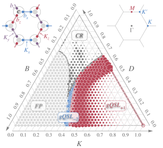
Figure 1: Phase diagram of Kitaev model with DM interaction under magnetic field. The full phase diagram of the Kitaev model in the presence of a magnetic field pointing in the $[1,1,1]$ direction ($t=1$) is shown. Empty regions indicate gapless phases and the size of the hexagonal symbols indicate the size of the gap. Gray areas correspond to the gapped fully polarized (FP) phase with Chern number $\nu=0$, the red to a gapped QSL with $\nu=+1$ denoted as gQSL₊₁. A gapped QSL with an unconventional Chern number of $\nu=-2$, termed gQSL_-2 (dark blue) occurs between the FP and the gQSL₊₁. Away the KQSL at $K=1$ (open circle), an ungapped QSL, uQSL (thick red line) with equal Berry phases at the two Dirac points occurs for $B=0$ and $K=1$ at a non-zero DM, $D<0.5$, which becomes the gQSL₊₁ around $D\sim 0.5-0.65$, to finally become gapless and non- topological at a larger $D$ (dark gray). In this region, CR refers to classical regimes, beyond the accessibility of the present theory. The left inset shows the Majorana decomposition of the model considered while the right inset shows the first Brillouin zone and symmetry points of the honeycomb lattice.

The full model is treated using Kitaev’s Majorana decomposition of the spin $S^{\alpha}=\frac{1}{4}(ib^{\alpha}c-i\frac{1}{2}\epsilon_{\alpha,\beta,\delta}b^{\beta}b^{\delta})$ kitaev where greek letters span the space dimensions $(x,y,z)$ and $\epsilon_{\alpha,\beta,\delta}$ is the Levi-Civita symbol (Fig. 1). In this notation, $b$ operators correspond to flux band variables while $c$ describes the itinerant Majorana fermions. These are in the presence of the three other localized Majoranas which act as gauge fluxes (see Fig. 3(a) for the dispersion relation of the pure Kitaev model).

Going away from the specific Kitaev point requires the proper consideration of the constraint on the number of fermions – four Majoranas per spin – that can be only achieved in average by introducing Lagrange multipliers $\{\lambda_{i}\}$:

$$H_{L} = \frac{i}{4}\sum_{i,\alpha}\lambda_{\alpha}\left[b^{\alpha}_{i}c_{i}+\frac{1}{2}\epsilon_{\alpha\beta\delta}b^{\beta}_{i}b^{\delta}_{i}\right]$$

where summation over repeated indices is assumed. The explicit implementation of the fermion constraint is crucial for a proper description of model (1) containing terms other than the pure Kitaev contribution and we have provided all details in suppl .

The complete phase diagram of model (1) can be nicely represented in a ternary plot as displayed in Fig. 1 for ${\bf B}$ in the $[1,1,1]$ direction ($t=1$) and ${\bf D}$ along the $z$-direction ($d=0$) for simplicity, realizing that the case $d=1$ is qualitatively similar. On this graph only, the full parameter range of the model onto the plane fulfills the constraint $K+D+B=1$, providing $K>0$, $D>0$ and $B>0$, the area of the hexagons is proportional to the gap at this point, and the color refers to different states of matter. In this ($K,D,B$) constrained space, the vertex defined by (0,0,1) corresponds to the topologically trivial ($\nu=0$) fully polarized (FP) state, (1,0,0), to the gapless Kitaev QSL (KQSL) and (0,1,0) to a gapless classical state whose magnetic properties remain yet to be determined. Three different topological phases characterized by their Chern numbers can be distinguished in the phase diagram. A gapped topological QSL with $\nu=+1$ denoted by gQSL₊₁ is topologically equivalent to the QSL found by Kitaev at weak magnetic fields. The novel gapped QSL with unconventional Chern number of $\nu=-2$ is denoted by gQSL_-2. The gray areas correspond to the FP state with $\nu=0$. The mechanisms driving these topological states are explained below, but we emphasize here the presence of the two novel gapped topological QSL with large Chern numbers, $\nu=\pm 2$. These are the result of the strong competition between the three terms entering the hamiltonian and occur in intermediate regions between the FP and the gQSL₊₁ phases. These phases are chiral QSLs since time reversal symmetry is broken either explicitly by the applied magnetic field or spontaneously for $B=0$ and $D\neq 0$. Interestingly, at zero field, $B=0$, a small but finite DM of $D\lesssim 0.5$ (with $K=1$) leads to equal Berry phases, $\phi_{k}$, around the Dirac nodes (see Fig. 1 for the first Brillouin zone of the lattice) $\phi_{K}=\phi_{K^{\prime}}=\pm\pi$ in contrast to the opposite Berry phases found in the pure Kitaev model, $\phi_{K}=-\phi_{K^{\prime}}=\pm\pi$. Hence, we have unraveled a new ungapped QSL with non-zero chirality which we denote by uQSL.

Applying a tilted magnetic field is found to open a gap in the Majorana fermion spectrum, consistent with perturbation theory kitaev . The gap is opened symmetrically with respect to the zero energy and the resulting gapped QSL is topological with a nonzero Chern number $\nu=\pm 1$, the sign depending on the direction of the magnetic field. Our gap arises naturally from imposing the constraints on the Majorana fermions in contrast to a previous Majorana mean field analysis which add by hand a three-spin term to be able to open a gap nasu . We associate the gap opening to the non-zero Lagrange multipliers (Novel chiral quantum spin liquids in Kitaev magnets) which lead to local hybridization between matter and flux Majorana fermions for $B\neq 0$. We note that the one-particle constraints are not automatically verified when considering models beyond the pure Kitaev model even at the mean-field level so it is necessary to impose them explicitly suppl . Hence, our MMFT is capable of describing correctly the exact KQSL at $B=0$ as well as the gapped QSL under low magnetic fields without making any extra assumptions. We finally note that closely related Abrikosov fermion mean-field theories gholke imposing the one single-particle constraint through a single Lagrange multiplier liu (our $\lambda_{z}$) instead of three choi – as we have done – can lead to different results to our MMFT suppl .

Concomitantly with the gap opening, the magnetic field leads to non-zero chiral currents of Majorana fermions between the n.n.n sites as shown in Fig. 2 (a). Only when the three components of the magnetic field are non-zero, all $\lambda_{\alpha}$ are simultaneously non-zero as well. This leads to hybridization among the four Majoranas at each site which ultimately leads to the gap opening. The size of the gap depends on $t$, the actual orientation of the magnetic field. When the field is parallel to one of the natural axis (say $t=0$ for ${\bf B}=Bu_{z}$), the gap is zero and we have a gapless QSL. At a critical $B$ we find that the $\pm\pi$ Berry phases at the Dirac points can switch their signs as found earlier nasu .

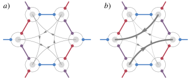
Figure 2: Chiral amplitudes in the Kitaev model from the Majorana mean-field theory. In (a) we show the n.n.n. chiral Majorana amplitudes, $\langle c_{i}c_{j}\rangle$, induced in the ground state MMFT wavefunction either by a magnetic field perpendicular to the plane, $t=1$, or a DM vector oriented perpendicular to the plane ($d=1$). These are responsible for the chiral QSL with Chern number $\nu=+1$ (gQSL₊₁) discussed in the text. (b) Anisotropic amplitudes (the thickness corresponds to the different strength) arising from finite DM $d\neq 1$ (with no applied magnetic field) responsible for the opening of the gap for $0.5<D<0.65$ (with $K=1$ and $d=0$) in the gQSL₊₁. The snapshots show one of the two possible chiralities of the ground state ($\nu=+1$). Note that (a) and (b) amplitudes are smoothly connected as shown in the phase diagram of Fig. 1.

We now discuss the effect of DM on the pure Kitaev model ($B=0$). As stated above, as the DM is increased the Berry phases around the Dirac points become equal: $\phi_{K}=\phi_{K^{\prime}}=\pm\pi$, indicating a change in the nature of the KQSL which characterizes the uQSL. As the $D$ parameter is further increased above a critical value, $D\gtrsim 0.5$ (with $B=0$ and $K=1$), the system opens up a gap leading to a topologically gapped chiral QSL with $\nu=\pm 1$ for either $d=0$ or $1$, gQSL_±1. The origin of the non-zero Chern number may be associated with the occurrence of anisotropic chiral amplitudes between n.n.n. sites as shown in Fig. 2(b) for $d<1$. This lattice nematicity induced by anisotropy of ${\bf D}$ is completely restored for $d=1$ at which the n.n.n. chiral amplitudes are the ones displayed in (a). In any case, the DM interaction induces both an ungapped and a gapped phase. This uQSL is a novel QSL which breaks TRS spontaneously in contrast with the gapped chiral QSL reported on the decorated honeycomb lattice yao due to its gapless character.

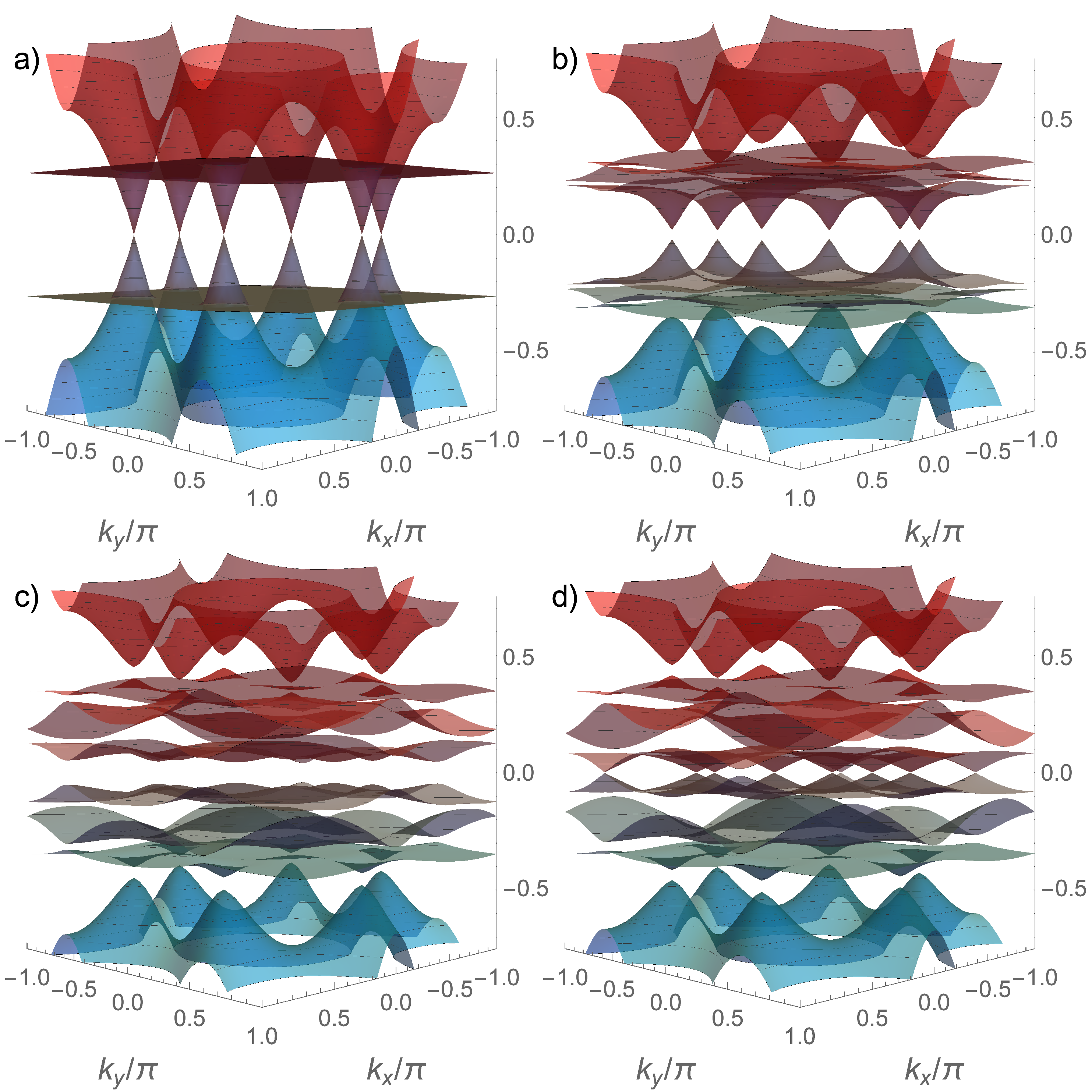
Figure 3: Majorana dispersions of the Kitaev model under a tilted external magnetic field and zero DM interaction. The evolution of the Majorana dispersions under a tilted $t=1$ magnetic field comparing the case (a) with no applied magnetic field, $B=0$, consisting of gapless Majorana dispersions and flat flux bands (three-fold degenerate) describing the Z₂ fluxes, (b) with $B\simeq 0.6$, where a gap has already opened and the flux Majorana bands remain flat. This gapped QSL with Chern number $\nu=+1$, gQSL₊₁, persists up to $B_{c}=1.43$ is adiabatically connected with the KQSL, (c) with $B=1.2$, the Dirac cones have been washed out and the gapped fluxes are strongly distorted becoming dispersive, (d) with $B=1.43$, a gapped QSL with $\nu=-2$, gQSL_-2, arises between $B_{c}$ and $B\simeq 1.64$ indicating a different topological state from the KQSL. $K\equiv 1$ in this plot.

When a $[001]$ magnetic field ($t=0$) is applied in the presence of a nonzero DM, a gapless QSL with the two Dirac cones shifted in opposite directions by the same amount occurs. The sublattice symmetry respected by the DM interaction protects Dirac cones from opening a gap. By tilting the magnetic field to $t=1$, a gap opens up as found in the case of zero DM leading to a gQSL_±1. But unlike opening symmetrically around zero, the gap centers are equally shifted in opposite directions at the two cones.
In Fig. 3 we show the evolution of the Majorana dispersions under a $[111]$ magnetic field ($t=1$). With no magnetic field applied the MMFT dispersions consist on gapless Majorana matter bands touching at the Dirac points and flat bands describing localized Z₂ fluxes. The flat bands are three-fold degenerate in this case. As the magnetic field increases up to about $B\sim 0.6$, (with $K=1$) a gap opens up at the Dirac points while the flux bands remain almost flat. This gQSL₊₁ phase – since it is gapped and $\nu=+1$ – is adiabatically connected to the gapped QSL found by Kitaev kitaev . As the magnetic field is increased up to $B_{c}\simeq 1.43$ the flux bands are gradually distorted becoming dispersive and strongly hybridized with the Majorana matter bands. Note also how the bands are becoming closer at the three $M$ points for $B\sim B_{c}$. As the field is increased beyond $B_{c}$, a gap opens up at this newly formed band touching $M$ points with Berry flux magnitudes larger than $\pi$ in contrast to typical Dirac cones. This can be attributed to the fact that the matter and flux Majoranas are now forming unseparable composite objects due to the strong hybridization in this magnetic field regime suppl . Hence, we find a gapped topological QSL with Chern number $\nu=-2$ emerging in the range $B\in[1.43,1.64]$. It is interesting to note that a CSL with $\nu=2$ has been found in liu but with an extra symmetric spin term in the hamiltonian. At larger magnetic fields ($B>1.64$) there is a transition to a gapped and fully polarized insulator with a trivial topology ($\nu=0$) – the full polarization is an artefact of the method. The Majorana dispersions are also strongly modified by $D$ even for $B=0$. Recent numerical studies yfjiang -trivedi suggest the existence of a gapless intermediate phase in a somewhat similar parameter range. In spite of the different features found (gapless vs. gapped), our gap closing around $B_{c}$ can be associated with the large enhancement of low energy excitations developing near the PL phase. Interestingly, we have supported by ED the fact that $D$ and $B$ combined possibly lead to a gap opening. All these points are detailed in suppl .

To conclude, we discuss our results in the context of Kitaev materials. Although they are mostly believed to have FM couplings jackeli ; winter ; valenti , some works suggest kee ; banerjee2017 AFM couplings as mostly considered here. QSL behavior has recently been observed in the honeycomb magnet H₃LiIr₂O₆ kitagawa with the caution that H disorder in this material can deviate magnetic couplings from the Kitaev model li ; vandenbrink . Although $\alpha$-RuCl₃ is magnetically ordered, there is experimental evidence for its proximity to a QSL phase banerjee2016 ; banerjee2017 . Under high pressure above 1 GPa wang2019 or applying a magnetic field destroys AF order giving way to a gapped QSL hentrich2018 ; baek2017 . Strikingly, recent thermal Hall conductivity experiments find fractional quantization of the thermal conductance which is attributed to the Majorana edge modes in a gQSL₊₁ motome . NMR experiments find a spin gap $\Delta\propto B^{3}$ at small fields ruegg due to the fractionalization of the spin into two gauge fluxes and a gapped Majorana fermion as predicted by Kitaev kitaev . Fig. 4 shows that a similar spin gap opening with a [111] magnetic field and zero DM should be observed in AFM Kitaev materials.

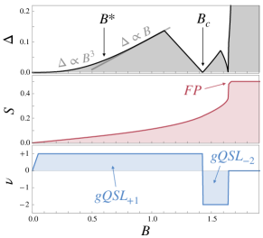
Figure 4: Dependence of the gap (top), the magnetic moment (middle) and the Chern number (bottom) with an applied magnetic field and zero DM interaction. The gap obtained from the MMFT changes from $\Delta\propto B^{3}$, expected from perturbation theory, to $\Delta\propto B$ around $B^{*}\sim 0.6$ under the magnetic field ${\bf B}=B(1,1,1)/\sqrt{3}$. A topological transition from a gapped QSL with Chern number, $\nu=+1$, gQSL₊₁, to a QSL with $\nu=-2$, gQSL_-2, occurs at $B_{c}\sim 1.43$. For $B\gtrsim 1.64$ a topologically trivial polarized insulator is stabilized. $K=1$ in this plot.

Fig. 4 also shows that in AFM Kitaev materials, the gQSL₊₁ (under a positive magnetic field) would survive up to an applied tilted magnetic field of $B\lesssim B_{c}$, way beyond the perturbative regime. The Majorana edge states in this QSL will contribute to the thermal Hall conductance kitaev ; nagaosa2012 , $\kappa_{xy}/T=\frac{\pi}{12}\frac{k_{B}^{2}}{\hbar d}$, as recently observed motome . This is half and opposite in sign to the thermal Hall conductance observed in an integer quantum Hall effect experiment kane1997 associated with electronic charge. Strikingly, since a distinct gapped QSL with $\nu=-2$ in the range $B\sim 1.43-1.64$ arises ($\sim$ 90 Tesla using $2K\approx 7$ meV for $\alpha$-Ru Cl₃), our analysis predicts a sudden jump of $\kappa_{xy}/T$, the thermal Hall coefficient, from $\frac{\pi}{12}\frac{k_{B}^{2}}{\hbar d}$ to $-\frac{\pi}{6}\frac{k_{B}^{2}}{\hbar d}$ around $B_{c}$. This signals a novel topological transition in AFM Kitaev magnets that could be searched experimentally.

Acknowledgements. J. M. acknowledges financial support from (RTI2018-098452-B-I00) MINECO/FEDER, Unión Europea, through the María de Maeztu Programme for Units of Excellence in R&D (CEX2018-000805-M) and from (mobility program: ”Salvador de Madariaga”: PRX18/00070) Ministerio de Educación, Cultura y deporte in Spain and the hospitality from Néel Institute in Grenoble. We thank anonymous referee for making us realize that the gap closing to the fully polarized state was overlooked in the first version.

I Details on the Majorana mean field theory

As mentioned in the main text, mapping the spins 1/2 onto four Majorana fermions can be seen as a two-step procedure. First we proceed to the standard parton construction by introducing two Abrikosov fermions:

$$S_{i}^{\alpha}=\frac{1}{2}f_{i}^{a+}\sigma^{\alpha}_{ab}f_{i}^{b}.$$ (2)

These two fermion species carry the magnetic moment of the spin, and for each of them, two Majorana fermions can be introduced as:

$$f_{i\uparrow} = \frac{1}{2}(c_{0}-ic_{3})$$

$$f_{i\uparrow}^{+} = \frac{1}{2}(c_{0}+ic_{3})$$

$$f_{i\downarrow} = \frac{1}{2}(c_{2}-ic_{1})$$

$$f_{i\downarrow}^{+} = \frac{1}{2}(c_{2}+ic_{1})$$ (3)

with the specific commutation relation $\{c_{i}^{a},c_{j}^{b}\}=2\delta_{ij}\delta_{ab}$. In the text, $c_{0}=c$, $c_{1}=b^{x}$, $c_{2}=b^{y}$ and $c_{3}=b^{z}$, but let’s keep the $c_{i}$ notation for simplicity. Defined like this, the spins read:

$$S_{i}^{x} = \frac{1}{2}\left[f_{i\uparrow}^{+}f_{i\downarrow}+f_{i\downarrow}^{+}f_{i\uparrow}\right]=\frac{1}{4}(+ic_{1}c_{0}+ic_{3}c_{2})$$

$$S_{i}^{y} = \frac{-i}{2}\left[f_{i\uparrow}^{+}f_{i\downarrow}-f_{i\downarrow}^{+}f_{i\uparrow}\right]=\frac{1}{4}(+ic_{2}c_{0}+ic_{1}c_{3})$$

$$S_{i}^{z} = \frac{1}{2}\left[f_{i\uparrow}^{+}f_{i\uparrow}-f_{i\downarrow}^{+}f_{i\downarrow}\right]=\frac{1}{4}(+ic_{3}c_{0}+ic_{2}c_{1})$$ (4)

and the single occupation constraints $f_{i\uparrow}^{+}f_{i\uparrow}+f_{i\downarrow}^{+}f_{i\downarrow}=1$, $f_{i\uparrow}^{+}f_{i\downarrow}^{+}=0$ and $f_{i\uparrow}f_{i\downarrow}=0$ (see below for discussion) yield to three additional terms to be introduced with corresponding Lagrange multipliers $\{\lambda_{i}\}$ in the model:

$$c_{3}c_{0}-c_{2}c_{1}=0,$$

$$c_{2}c_{0}-c_{1}c_{3}=0,$$

$$c_{1}c_{0}-c_{3}c_{2}=0.$$ (5)

Let’s now focus on the pure isotropic Kitaev model for illustrating how the method is implemented. Injecting the above defined mapping and considering the constraints to be fulfilled, the Hamiltonian can be cast as:

$$H_{K} = K\sum_{i\in u}\left[S_{i}^{x}S_{i+d_{1}}^{x}+S_{i}^{y}S_{i+d_{2}}^{y}+S_{i}^{z}S_{i+d_{3}}^{z}\right]$$ (6)

$$= -K\sum_{i\in u}\sum_{a=1}^{3}\frac{i}{2}c^{a}_{i}c^{a}_{i+d_{a}}\frac{i}{2}c^{0}_{i}c^{0}_{i+d_{a}}$$ (7)

This Hamiltonian can now be mean-field decoupled following three different channels of binilears:

$$(a) \to \langle\frac{i}{2}c^{a}_{i}c^{a}_{i+d_{a}}\rangle\frac{i}{2}c^{0}_{i}c^{0}_{i+d_{a}}+\frac{i}{2}c^{a}_{i}c^{a}_{i+d_{a}}\langle\frac{i}{2}c^{0}_{i}c^{0}_{i+d_{a}}\rangle$$

$$(b) \to -\langle\frac{i}{2}c^{a}_{i}c^{0}_{i}\rangle\frac{i}{2}c^{a}_{i+d_{a}}c^{0}_{i+d_{a}}-\frac{i}{2}c^{a}_{i}c^{0}_{i}\langle\frac{i}{2}c^{a}_{i+d_{a}}c^{0}_{i+d_{a}}\rangle$$

$$(c) \to \langle\frac{i}{2}c^{a}_{i}c^{0}_{i+d_{a}}\rangle\frac{i}{2}c^{a}_{i+d_{a}}c^{0}_{i}+\frac{i}{2}c^{a}_{i}c^{0}_{i+d_{a}}\langle\frac{i}{2}c^{a}_{i+d_{a}}c^{0}_{i}\rangle$$ (8)

and corresponding constant terms. The mean field Hamiltonian is then Fourier transformed with the specific form:

$$c_{i}^{a}=\frac{\sqrt{2}}{\sqrt{n_{s}}}\sum_{q}e^{iqr_{i}}c_{q}^{a}$$ (9)

where $n_{s}$ is the number of Bravais sites in the lattice and the extra $\sqrt{2}$ allows for recovering standard fermionic commutation relations in $q$-space:

$$\sum_{i}\{c_{i}^{a}c_{i}^{a}\} = \sum_{q}c_{q}^{a}c_{-q}^{a}+c_{-q}^{a}c_{q}^{a}=n_{s}$$

$$\sum_{q}c_{q}^{a}c_{q}^{a} = 0,$$ (10)

where $c_{-q}^{a}$ can be identified to the creation operator $c_{q}^{a+}$. Thus, in the reciprocal space, the Majoranas follow the rules $\{c_{q}^{a},c_{q^{\prime}}^{b}\}=\{c_{q}^{a+},c_{q^{\prime}}^{b+}\}=0$ and $\{c_{q}^{a},c_{q^{\prime}}^{b+}\}=\delta_{q,q^{\prime}}\delta_{a,b}$ as standard fermions. Then, one can simply diagonalize the mean field Hamiltonian with all terms decoupled as previously shown in the single particle basis. The set of Lagrange multipliers $\{\lambda_{i}\}$ are fixed by imposing the single occupancy constraint given by Eq. (5), at the mean-field level only, using a least square minimization. This done, we obtain the mean field many-body wave function by constructing a Slater determinant up to half-filling. The operators of the type $\frac{i}{2}c_{i}^{a}c_{j}^{b}$ are then computed in this ground state and re-injected in the mean field hamiltonian leading to a set of self-consistent equations (SCE) which are solved numerically without imposing any restrictions on the mean-field solutions. We repeat this procedure until convergence of the mean field parameters and the energy up to a desired tolerance $\delta$ is achieved. In our case, we have fixed this tolerance to at least $\delta=10^{-10}$ on the parameters. Calculations are performed following a Broyden minimization method broyden up to $60\times 60$ clusters which are sufficiently large to describe the behavior of the model in the thermodynamic limit.

All mean field parameters are in the ground state Slater determinant of the Majoranas, providing an efficient and stable way to converge towards the saddle points. Our construction easily deals with enlarged unit-cells (we have checked our results up to 12 site unit-cells) which allows for higher symmetry breaking mean- field solutions which could be overlooked in too small clusters. This is for instance the case of the zig-zag and stripy phases reported in the next section when the Heisenberg exchange term is added to the system.

In contrast to other Majorana mean-field theories, our approach imposes the single occupancy constraint on average throughout the full phase diagram. The differences between our approach and a close mean-field theorynasu which uses a two-Majorana representation per site is provided in Section. V of the present Supplementary Material together with the comparison with alternative approaches based on Abrikosov fermions schaffer ; liu . The possibility of explicitly having four occupied bands as in our MMFT, three associated with the gauge fluxes and one with the matter provides more insights about the nature of the different phases in contrast to having only two occupied bands nasu . An augmented parton construction has also been proposedknolle , in a model in which the constraint has not been violated. This approach is designed for the description of the dynamics of the excitations above the ground state energy in the Kitaev $+\Gamma$ term.

II Heisenberg-Kitaev Phase diagram

As mentioned in the main text, the magnetic orders observed in candidate materials of the Kitaev model indicate the presence of Heisenberg like interactions and even other types of exchanges. Before studying in detail the phase diagram under a magnetic field and the DM interaction, we have verified that our self-consistent MMFT with constraints can reproduce the phase diagram of the Heisenberg-Kitaev model found through exact numerical techniqueschaloupcka ; trebst2011 .

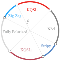
Figure 5: Phase diagram of the Heisenberg-Kitaev model obtained from the MMFT as a function of $\theta$. The extension of the two Kitaev QSL, labeled KQSL₁ and KQSL₂ is very large. The pure Kitaev point at $\theta=0$ is in the middle of KQSL₁. Different magnetic orders, compatible with those already reported in the literature, are obtained by enlarging the number of sites per unit cell in our theory, e.g. the Zig-Zag and the Stripy phases.

Thus, we have considered the hamiltonian $H=H_{K}+H_{J}$ with $H_{K}=2K\sum_{\langle i,j\rangle,\gamma}S_{i}^{\gamma}S_{j}^{\gamma}$ and $H_{J}=J\sum_{\langle i,j\rangle}{\bf S}_{i}\cdot{\bf S}_{j}$. We then introduce the extrapolation parameter $\theta$ defined as $\tan\theta=J/K$ and solve the self-consistent equations of our theory for $\theta\in[0,2\pi]$. The corresponding phase diagram is displayed in Fig.5. Note that we have considered theories up to four sites per unit cell, necessary to stabilize large unit-cell magnetic orders such as the Zig-Zag and the Stripy phases lesphases .

The good agreement with other techniques indicates the relevance of the method and its capability of treating magnetic orders and QSL phases on equal footing. In addition, we see that the pure Kitaev limit ($\theta=0$) lies deep in the domain of the Kitaev QSL (1) (KQSL₁), and since we are interested in the effects of the magnetic field and Dzyaloshinskii-Moriya interactions on this QSL, we can restrict our analysis to this $\theta=0$ starting point without any loss of generality.

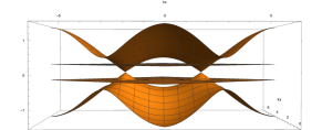
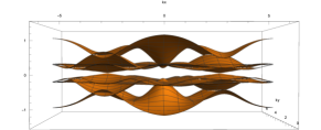
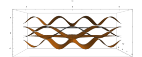
Figure 6: Majorana dispersions of the Kitaev model in the presence of the DM interaction. The dependence of the Majorana dispersions with DM with no applied magnetic field, $B=0$, is shown. At a finite DM fo $D=1.4$ (top panel) the Majorana dispersions resemble the bare dispersions of the KQSL in which the linear Majorana dispersions and the flat flux bands are evident. However, the Berry phases around the Dirac points are equal. As the DM is increased up to $D=1.5$ a gap opens up in the spectrum and a gapped QSL with $\nu=-1$, gQSL_-1 emerges. The whole spectrum of this state is strongly modified due to strong hybridization between the flux and itinerant Majoranas and the Dirac points located at $K$ and $K^{\prime}$ in the pure Kitaev model ($D=0$) move to new locations in the Brillouin zone. The bottom panel shows the dispersions at even larger values, $D=1.6$, in which the system is going into a gapless state.

III Effect of Dzyaloshinskii-Moriya interaction on Majorana spectrum

As discussed in the main text, the DM interaction has an important effect on the ground state of the pure Kitaev model i. e. the KQSL. Even with no applied magnetic field, a small but finite DM can induce a transition from a KQSL to an uQSL. The uQSL is a chiral QSL which is characterized by having the two Berry phases around the Dirac cones equal to $+\pi$ or to $-\pi$ in contrast to the KQSL. At sufficiently large $D$ and with $B=0$ a transition to a gQSL_-1 (see the phase diagram shown in Fig. 1 of the main text) occurs. In order to analyze this transition we show in Fig. 6 the change in the Majorana spectrum with increasing $D$.

IV Multiband Berry phase and Chern number

The Berry phases and Chern numbers determining the topological properties of the model are obtained numerically using a multiband approach. This is necessary since the itinerant and flux Majorana bands are occupied. This is done by defining the overlap matrix $M_{mn}^{({\bf k}_{j},{\bf k}_{i})}=\langle u_{m,{\bf k}_{j}}|u_{n,{\bf k}_{i}}\rangle$, with $m,n=1,...,N_{b}$ band indices and ${\bf k}_{i}$ are discrete momenta of the first Brillouin zone. We define the matrix $U({\bf k}_{0})=\prod_{j=0}^{N-1}M_{mn}^{({\bf k}_{j},{\bf k}_{j+1})}$ around a closed path in the BZ encircling a point ${\bf q}$ of interest, where successive steps in momentum around the loop are taken. Note that ${\bf k}_{N}={\bf k}_{0}$ for closing the loop. The Berry phase then reads $\phi({\bf q})=\text{Im}\ln|U({\bf k}_{0})|$. The Chern number is immediately obtained from this expression by discretising the first Brillouin zone in elementary four-site plaquettes fukui (${\bf k}_{j}\to{\bf k}_{j}+{\bf u}_{1}\to{\bf k}_{j}+{\bf u}_{1}+{\bf u}_{2}\to{\bf k}_{j}+{\bf u}_{2}\to{\bf k}_{j}$) and defining the Berry flux matrix $F({\bf k}_{j})=\text{Im}\ln\left|U({\bf k}_{j})\right|$ on each of them. The total Chern number $\nu$ of the system is then nothing else but the sum of all the Berry fluxes over the whole BZ as $\nu=\frac{1}{2\pi}\sum_{j}F({\bf k}_{j})$ and so the thermal Hall coefficient is half-quantized as: $\frac{\kappa_{xy}}{T}=\frac{\pi}{12}\frac{k_{B}^{2}}{\hbar d}\nu$.

V Effect of the single-occupancy constraint

One key feature of our Majorana parton approach stands in the appropriate implementation of the single particle constraint to deal with the Kitaev model under the magnetic field and the DM interaction. We now discuss the effect of the single occupancy constraint, needed to recover the right spin operators from the Majorana fermions, on the magnetic properties of the Kitaev model under an external magnetic field. Following kim , in our MMFT we have imposed (on average) the condition of single particle occupation leading to the following three constraints on the Majorana fermions:

$$\langle ib^{x}c\rangle-\langle ib^{z}b^{y}\rangle=0,$$

$$\langle ib^{y}c\rangle-\langle ib^{x}b^{z}\rangle=0,$$

$$\langle ib^{z}c\rangle-\langle ib^{y}b^{x}\rangle=0.$$ (11)

This is in contrast with certain MMFT which do not impose these constraints (on average) explicitly nasu but assume that within the two Majorana representation of the spin operators obtained through a Jordan Wigner transformation they are automatically satisfied. However, we show how this assumption is only valid in the pure Kitaev model. Within our MMFT we use a four Majorana representation of the spins: $S^{\alpha}=ib^{\alpha}c$, which implicitly also assumes that the single occupancy constraint given by the conditions over the Majorana fermions $b^{x}c=b^{z}b^{y},b^{y}c=b^{x}b^{z},b^{z}c=b^{y}b^{x}$, is satisfied as in previous approaches. However, as we discuss below, we have checked that the above constraints are only satisfied in the pure Kitaev model i.e. when no magnetic field nor other exchange interactions are considered. Hence, we found necessary in our MMFT to impose the constraints (11) in order to recover the one-particle condition per site at least on average.

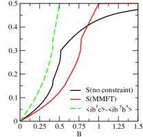
Figure 7: Effect of removing the single occupancy constraint on the dependence of the magnetic moment with an applied magnetic field. The dependence of the magnetic moment, $S$, on a magnetic field in the $[001]$ direction applied to the Kitaev model with no DM interaction, $D=0$, is shown. The results obtained from our MMFT with the constraints (11) are compared with the results in which no constraints are imposed. The dependence of the constraint with the field shows how it is strongly violated as the magnetic field is increased. $K=0.5$ in this plot. Calculations are performed on a $36\times 36$ cluster.

In Fig. 7 we show results obtained within our MMFT with the constraints (11) fulfilled and compared with the case in which they have been removed. The MMFT without constraints recovers the dependence of the magnetic moment with a $[001]$ magnetic field reported previously in the literature nasu . Namely a transition from a gapless phase to another gapless phase at which the $\pm\pi$ Berry phases associated with the two Dirac cones switch their sign occurs around $B=0.42$ and a second transition to a gapped polarized phase occurs at $B=0.52$. When the constraints are imposed though, these three different phases are present but their critical transition values are shifted. Also we find that the polarized phase is fully saturated in contrast to the case when no constraints are imposed.

Let’s discuss the effect of the constraints when a magnetic field is applied in the $[111]$ direction. In Fig. 8 we compare the magnetic moment and the gap with and without the constraints imposed. The first important difference between the two approaches is that while our MMFT (with the constraints imposed) naturally recovers the topological gapped phase (with Chern number, $\nu=\pm 1$) even at small magnetic fields $B$, as found by Kitaev. In contrast, the system is gapless up to $B\sim 1.4$ in the no-constraint MMFT. In order to recover Kitaev’s gapped topological phase, three spin terms arising in perturbation theory to O($B^{3}$) need to be added by hand to the Kitaev model nasu . Hence, imposing the constraint is readily essential for recovering the correct behavior of the Kitaev model under a $[111]$ magnetic field in any regime of the magnetic field. Importantly, no topological phases are found when the constraints are not imposed. While the two Berry phases around the Dirac cones have opposite signs, $\pm\pi$, in the ungapped phase for $B\lesssim 1.4$, the gapped phase found for $B\gtrsim 1.4$ is trivial, $\nu=0$, as shown in Fig. 8. Finally, without the constraints, there are n signatures of the $\nu=-2$ topological phase found with our MMFT (Fig. 4 of the main text).

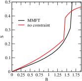
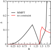
Figure 8: Effect of removing the single occupancy constraint on the dependence of the magnetic moment and the gap with an applied magnetic field. The dependence of the magnetic moment, $S$, and the gap on a $[111]$ magnetic field applied to the Kitaev model with no DM interaction, $D=0$, is shown. The results obtained from the MMFT with the constraints (11) included are compared with the results in which no single occupancy constraints imposed. No gap opening is found for $B\lesssim 1.4$ when the constraints are removed. $K=1$ in this plot. Calculations are performed on a $36\times 36$ cluster.

We finally discuss the relationship between our MMFT theory and mean-field decompositions based on Abrikosov fermions. gholke ; liu It has been shown kim how a faithful Abrikosov fermion mean-field theory of the Kitaev model can be obtained after performing a unitary rotation on a Majorana mean-field hamiltonian similar to ours i. e. using the spin operators: $S_{\alpha}=b_{\alpha}c$, so the Majorana constraint $D=b_{x}b_{y}b_{z}c=1$ at each site is automatically satisfied with both spin liquid and magnetic channels taken into account. The derived Abrikosov fermion hamiltonian contains mean-field terms of the pairing type associated with the QSL channel and of the magnetic type as well as three constraints implying three Lagrange multipliers. Such mean-field construction not only leads to the correct exact KQSL and correct ground state energy when $B=0$ but also treats more accurately the QSL channels at non-zero $B$ as compared to conventional mean-field Abrikosov fermion decompositions which introduce only one Lagrange multiplier (our $\lambda_{z}$) associated with the condition: $n_{i}=\sum_{\sigma}f^{\dagger}_{i\sigma}f_{i\sigma}=1$ (where $f^{\dagger}_{i},f_{i}$ the Abrikosov fermions) on average liu . Since, at the mean-field level, our MMFT and a conventional Abrikosov fermion approach deal with the particle number constraint in different ways one should expect different results. However, it is still interesting to note that a CSL with Chern number $\nu=\pm 2$ has been found in liu when ${\bf B}||{\bf c}$ (i. e. along the $[111]$ direction) which is consistent with our gQSL_-2 phase although their model liu contains an extra symmetric spin term that we do not include in our hamiltonian.

VI Comparison to Exact Diagonalization

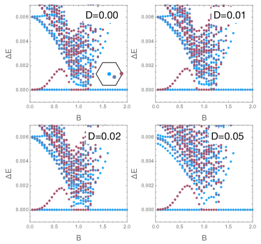
Figure 9: Gap spectra versus $B$ in the $[111]$ direction for various $D$ obtained by ED on a 18 site cluster. The first 10 levels are displayed in the three inequivalent symmetry sectors (see inset) at the $\Gamma$ (light blue), $X$ (dark blue) and $K$ (red) points. As $D$ increases from 0 to 0.05, the gap in the intermediate phase, defined by the change of the ground state symmetry sector, grows, in agreement with our MMFT results. Hence, gap opening in the thermodynamic limit cannot be excluded for any finite $D$.

In order to challenge our gQSL_-2 phase, we have computed the gap spectra of the model by exact diagonalizations (ED) on a 18 site cluster, for 4 different values of $D$, in function of $B$ along the $[111]$ direction and using the translational symmetries (Fig. 9). As found in previous studies trebst2019 ; trivedi , the intermediate phase defined by the change of symmetry in the ground state, is expected to be gapless, even though larger cluster sizes should be analyzed to reach a definitive conclusion about the gap opening in the thermodynamic limit. However, for a cluster of 32 sites trebst2019 , a significant shrinking of the energy excitations lets suggest that the gap might be vanishing at the thermodynamic limit.

We are here interested on the behavior of the spectrum of the intermediate phase under the presence of the DM term. As we have obtained in the MMFT, the gQSL_-2 extends in the parameter space for finite K, D and B, and is always gapped. In our ED results, starting from $D=0$ (upper-left panel) and slowly increasing $D$, a clear increasing of the gap between the ground state energy and the first excited state is observed. A finite size scaling would be necessary for being definitely conclusive about a possible gap opening, but we clearly show here that the combined effect of $D$ and $B$ tends to increase the gap which is in good agreement with our MMFT.

The second effect of this combination is the location of the boundaries of the intermediate phase. As $D$ increases, they are pushed to higher magnetic field, a tendency that is also reproduced by our MMFT.

Since the gap we have found in the gQSL_-2 when $D=0$ is very small in comparison with the one in the gQSL₊₁ phase or the polarized phase, it is not inconsistent with ED calculations, as these cannot exclude the presence of a tiny gap in the thermodynamic limit. Moreover, the behavior of the intermediate phase (change of symmetry, $D$ vs. $B$, gap increasing) in ED agrees with our phase diagram of Fig. 1 in our manuscript. This gives further support to the existence of our intermediate gQSL_-2 phase, which should be gapped when $D$ and $B$ are combined lunkin . As pointed out above, we cannot exclude that, for $D=0$, the gap indeed closes in the thermodynamic limit as suggested by exact numerical treatments on small systems trebst2019 ; trivedi .

VII Topological phase transitions from multiband Chern numbers

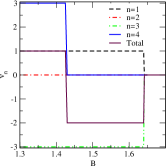
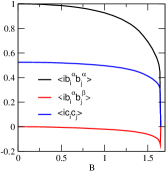
Figure 10: Dependence of Chern numbers and Majorana bond averages on the magnetic field. In the left plot the decomposition of the total Chern number, $\nu$, into its band contributions $\nu_{n}$, for different applied magnetic fields, ${\bf B}=B(1,1,1)/\sqrt{3}$, and no DM ($D=0$) are shown. The suppression of the total Chern number, $\Delta\nu=-3$, is found to be solely due to the change in the Chern number in the fourth band, $\Delta\nu_{4}=-3$. In the right plot, the Majorana bond averages as a function of $B$ are shown.

Further insight into the topological phase transitions occurring at $B_{c}=1.43$ and $B=1.64$ when no DM interaction is present (see Fig. 4 of the main text) can be obtained by computing the Chern number, $\nu_{n}$, of the four lowest Majorana bands as shown in Fig. 10 for a system size of $72\times 72$ sites. At the phase transition from the gQSL₊₁ to the gQSL_-2 at $B_{c}$ the drop in the total Chern number, $\nu$ of 3 (with $\nu=\sum_{n}\nu_{n}$), can be attributed solely to the change in the Chern number of the highest occupied band from $\nu_{4}=3$ to $\nu_{4}=0$. Regarding the second transition from the gQSL_-2 to the polarized phase, Fig. 10 shows how at $B=1.64$ the Chern numbers of all bands drop simultaneously to zero, $\nu_{n}=0$, indicating the emergence of the polarized phase. In order to rationalize the changes in the topological properties of the system we have analyzed the dependence of the variational parameters with the applied field ${\bf B}=B(1,1,1)/\sqrt{3}$. The average Majorana bond values shown in Fig. 10, $\langle ib^{\alpha}_{i}b^{\alpha}_{j}\rangle$, are suppressed with $B$. For $B=0$, $\langle ib^{\alpha}_{i}b^{\beta}_{j}\rangle=\delta_{\alpha,\beta}$, recovering the exact zero-flux state of the localized Majorana fermions found by Kitaev. As $B$ increases $\langle ib^{\alpha}_{i}b^{\alpha}_{j}\rangle$ is only slightly suppressed, $\langle ib^{\alpha}_{i}b^{\alpha}_{j}\rangle\lesssim 1$ for $B\lesssim 0.5$. However, for larger $B>1$ it is rapidly suppressed and $\langle ib^{\alpha}_{i}b^{\beta}_{j}\rangle<0$ indicating that hybridization between different Majoranas localized at the n.n sites occurs. The strong suppression of $\langle ib^{\alpha}_{i}b^{\alpha}_{j}\rangle$ with $B$ indicates significant deviations from Kitaev’s zero-flux state with the generation of non-zero $Z_{2}$ fluxes which become itinerant (see how the flat bands in Fig. 3 of the main text gain dispersion with $B$). Hence, the jump of the Chern number around $B_{c}=1.43$ can be associated with such strong suppression. Indeed, the three localized bands, $n=1,2,3$, associated with the bond Majorana fermions give zero contribution to the Chern number: $\nu_{1}+\nu_{2}+\nu_{3}=0$ when $B=0$, as it should, since there are no non-zero Z₂ fluxes present in the KQSL. However, the non-zero Z₂ fluxes generated as $B$ is increased, lead to an uncompensated contribution of these bands to the total Chern number, $\nu_{1}+\nu_{2}+\nu_{3}=-3$, and a total Chern number, $\nu=-2$ when $B>B_{c}=1.43$. Although the matter Majorana bond averages $\langle ic_{i}c_{j}\rangle$ are also influenced by $B$ and display a suppression with $B$ as shown in Fig. 10, their relevance on the topological transition and Chern number changes seems to be only minor since these do not participate directly on the Z₂ flux dynamics.

References

- (1) L. Balents, Spin liquids in frustrated magnets, Nature 464, 199 (2010).
- (2) L. Savary and L. Balents, Quantum spin liquids: a review, Rep. Prog. Phys. 80, 016502 (2017).
- (3) P. W. Anderson, Resonating valence bonds: A new kind of insulator?, Mater. Res. Bull. 8 (2): 153 (1973).
- (4) G. Jackeli and G. Khalliulin, Mott Insulators in the Strong Spin-Orbit Coupling Limit: From Heisenberg to a Quantum Compass and Kitaev Models, Phys. Rev. Lett. 102, 017205 (2009).
- (5) H. Takagi, T. Takayama, G. Jackeli, and G. Khaliullin, Kitaev quantum spin liquid-concept and materialization, Nat. Rev. Phys. 1, 264 (2019).
- (6) K. Kitagawa, et. al. A spin-orbital entangled quantum liquid on honeycomb lattice, Nature 554, 341 (2018).
- (7) G. Y., Masashiko, H. Fujita, and M. Oshikawa Designing Kitaev spin liquids in metal-organic frameworks, Phys. Rev. Lett. 119, 057202 (2017).
- (8) A. Kitaev, Anyons in an exactly solvable model and beyond, Ann. Phys. 321, 2-111 (2006).
- (9) Y. Kasahara, et. al., Majorana quantization and half-integer thermal quantum Hall effect in a Kitaev spin liquid, Nature 559, 227 (2018).
- (10) N. Jansa, et. al. Observation of two types of fractional excitation in the Kitaev honeycomb magnet, Nat. Phys. 14, 786 (2018).
- (11) Y. F. Jiang, T. P. Devereaux, and H.-C. Jiang, Field-induced quantum spin liquid in the Kiatev-Heisenberg model and its relation to -RuCl3, Phys. Rev. B 100, 165123 (2019).
- (12) H.-C. Jiang,C.-Y. Wang, B. Huang, and Y.-M. Lu, Field induced quantum spin liquid with spinon Fermi surfaces in the Kitaev model, arXiv:1809.08247v2.
- (13) L. Zou, and Y.-C. He, Field-induced neutral Fermi surface and QCD3-Chern-Simons quantum criticalities in Kitaev materials, arXiv:1809.09091v2.
- (14) C. Kickey, and S. Trebst, Emergence of a field-driven U(1) spin liquid in the Kitaev honeycomb model, Nat. Comm. 10, 1038 (2019).
- (15) Z. Zhu, I. Kimchi, D. N. Sheng, and L. Fu, Robust non-Abelian spin liquid and a possible intermediate phase in the antiferromagnetic Kitaev model with magnetic field, Phys. Rev. B 97, 241110 (R) (2018).
- (16) R. Schaffer, S. Bhattacharjee, and Y. B. Kim, Quantum phase transition in Heisenberg-Kitaev model, Phys. Rev. B 86, 224417 (2012).
- (17) J. Knolle, S. Bhattacharjee, and R. Moessner, Dynamics of a quantum spin liquid beyond integrability: The Kiatev-Heisenberg- model in an augmented parton mean-field theory, Phys. Rev. B 97, 134432 (2018).
- (18) M. Gohlke, G. Wachtel, Y. Yamaji, F. Pollmann, and Y. B. Kim, Quantum spin liquid signatures in Kitaev-like frustrated magnets, Phys. Rev. B 97, 075126 (2018).
- (19) S. M. Winter, Y. Li, H. O. Jeschke, and R. Valentí, Challenges in design of Kitaev materials: Magnetic interactions from competing energy scales, Phys. Rev. B 93, 214431 (2016).
- (20) A. V. Lunkin, K. S. Tikhonov, M. V. Feigel’man, Perturbed Kitaev model: excitation spectrum and long-ranged spin correlations, Jour. of Phys. and Chem. of Sol. 128, 130, (2017).
- (21) We have mapped out the phase diagram of the Heisenberg-Kitaev model confirming the presence of an extended KQSL phase (see Supplementary material suppl ). Without loss of generality, we can thus restrict our study to the pure Kitaev case.
- (22) N. B. Perkins, Y. Sizyuk, and P. Wölfle., Interplay of many-body and single-particle interactions in iridates and rhodates, Phys. Rev. B 89, 035143 (2014).
- (23) See Supplemental Material at http://link.aps.org/supplemental/ for (i) details of the Majorana Mean Field Theory, (ii) the extension to the Heisenberg-Kitaev model (iii) the effect of the DM interaction on the Majorana spectrum, (iv) the computation of the multiband Berry phases and Chern numbers, and (v) the effect of the single-occupancy constraint on magnetic properties of the model. It includes references chaloupka ; fukui ; broyden ; trebst2011 ; lesphases .
- (24) J. Nasu, Y. Kato, Y. Kamiya, and Y. Motome, Succesive Majorana topological transitions driven by a magnetic field in the Kitaev model, Phys. Rev. B 98, 060416 (R) (2018).
- (25) Z.-X. Liu and B. Normand, Dirac and chiral quantum spin liquids on the honeycomb lattice in a magnetic field, Phys. Rev. Lett. 120, 187201 (2018).
- (26) W. Choi, P. W. Klein, A. Rosch, and Y. B. Kim, Topological superconductivity in the Kondo-Kitaev model, Phys. Rev. B 98, 155123 (2018).
- (27) H. Yao, and S. A. Kivelson, Exact chiral spin liquid with non-abelian anyons, Phys. Rev. Lett. 99, 247203 (2007).
- (28) S. Pradhan, N. D. Patel, and N. Trivedi, Two-Magnon Bound States in the Kitaev model in a [111]-field, arXiv:1908.10877.
- (29) S. M. Winter, A. A. Tsirlin, M. Daghofer, J. van den Brink, Y. Singh, P. Gegenwart, and R. Valentí, Models and materials for generalized Kitaev magnetism, J. Phys.: Condens. Matter 29, 493002 (2017).
- (30) H.-S. Kim, V. Shankar, A. Catuneanu, and H.-Y. Kee, Kitaev magnetism in honeycomb RuCl3 with intermediate spin-orbit coupling, Phys. Rev. B 91, 241110 (R) (2015).
- (31) A. Banerjee, et al., Neutron scattering in the proximate quantum spin liquid -RuCl3, Science 356, 1055 (2017).
- (32) Y. Li, S. M. Winter, and R. Valentí, Role of hydrogen in the spin-orbital-entangled quantum liquid candidate H3LiIr2O6, Phys. Rev. Lett. 121, 247202 (2018).
- (33) R. Yadav, et. al., Strong effect of hydrogen order on magnetic kitaev interactions in H3LiIr2O6, Phys. Rev. Lett. 121, 197203 (2018).
- (34) A. Banerjee, et. al., Proximate Kitaev quantum spin liquid behaviour in a honeycomb magnet, Nat. Mat. 15, 733 (2016).
- (35) Z. Wang,et. al., Pressure-induced melting of magnetic order and emergence of a new quantum state in -RuCl3, Phys. Rev. B 97, 245149 (2019).
- (36) R. Henritch, et. al., Unusual phonon heat transport in -RuCl3: strong spin-phonon scattering and field-induced spin gap, Phys. Rev. Lett. 120, 117204 (2018).
- (37) S.-H. Baek, S.-H. Do, K.-Y. Choi, Y. S. Kwon, A. U. B. Wolter, S. Nishimoto, J. van den Brink, and B. Büchner, Evidence for a field-induced quantum spin liquid in -RuCl3, Phys. Rev. Lett. 119, 037201 (2017).
- (38) K. Nomura, S. Ryu, A. Furusaki, and N. Nagaosa, Cross-correlated responses of topological superconductors and superfluids, Phys. Rev. Lett. 108, 026802 (2012).
- (39) C. L. Kane and M. P. A. Fisher, Quantized thermal transport in the fractional quantum Hall effect, Phys. Rev. B 55, 15832 (1997).
- (40) J. Dennis, J. Moré, Quasi-Newton Methods, Motivation and Theory, Society for Industrial and Applied Mathematics 19, 46 (1977).
- (41) Chaloupka, J., Jackeli, G., and Khaliullin, G., Kitaev-Heisenberg Model on a Honeycomb Lattice: Possible Exotic Phases in Iridium Oxides A2IrO3, Phys. Rev. Lett. 105 027204 (2010).
- (42) H.-C. Jiang, Z.-C. Gu, X.-L. Qi, and S. Trebst, Possible proximity of the Mott insulating iridate Na2IrO3 to a topological phase: Phase diagram of the Heisenberg-Kitaev model in a magnetic field, Phys. Rev. B 83, 245104 (2011).
- (43) D. Gotfryd, et. al., Phase diagram and spin correlations of the Kitaev-Heisenberg model: Importance of quantum effects, Phys. Rev. B 95, 024426 (2017).
- (44) Fukui, T., Hatsugai, Y., and Suzuki, H., Chern numbers and discretized Brillouin zone: efficient method of computing (spin) Hall conductances, Jour. of Phys. Soc. Jpn. 74, 1674 (2005).

References

- (1) J. Dennis, J. Moré, Quasi-Newton Methods, Motivation and Theory, Society for Industrial and Applied Mathematics 19, 46 (1977).
- (2) J. Nasu, Y. Kato, Y. Kamiya, and Y. Motome, Successive Majorana topological transitions driven by a magnetic field in the Kitaev model, Phys. Rev. B 98, 060416 (R) (2018).
- (3) R. Schaffer, S. Bhattacharjee, and Y. B. Kim, Quantum phase transition in Heisenberg-Kitaev model, Phys. Rev. B 86, 224417 (2012).
- (4) Z.-X. Liu and B. Normand, Dirac and chiral quantum spin liquids on the honeycomb lattice in a magnetic field, Phys. Rev. Lett. 120, 187201 (2018).
- (5) J. Knolle, S. Bhattacharjee, and R. Moessner, Dynamics of a quantum spin liquid beyond integrability: The Kitaev-Heisenberg- model in an augmented parton mean-field theory, Phys. Rev. B 97, 134432 (2018).
- (6) J. Chaloupka, G. Jackeli, and G. Khaliullin, Kitaev-Heisenberg Model on a Honeycomb Lattice: Possible Exotic Phases in Iridium Oxides A2IrO3, Phys. Rev. Lett. 105 027204 (2010).
- (7) H.-C. Jiang, Z.-C. Gu, X.-L. Qi, and S. Trebst, Possible proximity of the Mott insulating iridate Na2IrO3 to a topological phase: Phase diagram of the Heisenberg-Kitaev model in a magnetic field, Phys. Rev. B 83, 245104 (2011).
- (8) D. Gotfryd, et. al., Phase diagram and spin correlations of the Kitaev-Heisenberg model: Importance of quantum effects, Phys. Rev. B 95, 024426 (2017).
- (9) T. Fukui, Y. Hatsugai, and H. Suzuki, Chern numbers and discretized Brillouin zone: efficient method of computing (spin) Hall conductances, Jour. of Phys. Soc. Jpn. 74, 1674 (2005).
- (10) W. Choi, P. W. Klein, A. Rosch, and Y. B. Kim, Topological superconductivity in the Kondo-Kitaev model, Phys. Rev. B 98, 155123 (2018).
- (11) M. Gholke, G. Wachtel, Y. Yamaji, F. Pollmann, and Y. B. Kim, Quantum spin liquid signatures in Kitaev-like frustrated magnets, Phys. Rev. B 97, 075126 (2018).
- (12) C. Kickey, and S. Trebst, Emergence of a field-driven U(1) spin liquid in the Kitaev honeycomb model, Nat. Comm. 10, 1038 (2019).
- (13) S. Pradhan, N. D. Patel, and N. Trivedi, Two-Magnon Bound States in the Kitaev model in a [111]-field, arXiv:1908.10877.
- (14) A. V. Lunkin, K. S. Tikhonov, and M. V. Feigel’man, Perturbed Kitaev model: excitation spectrum and long-ranged spin correlations, Jour. of Phys. and Chem. of Sol. 128, 130 (2017).