Propagating geometry information to finite element computations

Abstract

The traditional workflow in continuum mechanics simulations is that a geometry description – for example obtained using Constructive Solid Geometry or Computer Aided Design tools – forms the input for a mesh generator. The mesh is then used as the sole input for the finite element, finite volume, and finite difference solver, which at this point no longer has access to the original, “underlying” geometry. However, many modern techniques – for example, adaptive mesh refinement and the use of higher order geometry approximation methods – really do need information about the underlying geometry to realize their full potential. We have undertaken an exhaustive study of where typical finite element codes use geometry information, with the goal of determining what information geometry tools would have to provide. Our study shows that nearly all geometry-related needs inside the simulators can be satisfied by just two “primitives”: elementary queries posed by the simulation software to the geometry description. We then show that it is possible to provide these primitives in all of the commonly used ways in which geometries are described in common industrial workflows. We illustrate our solutions using examples from adaptive mesh refinement for complex geometries.

1 Introduction

The traditional workflow of finite element, finite volume, and finite difference simulations of physical processes consists of three phases: what is called “preprocessing”; the actual numerical solution of a partial differential equation; and what is called “postprocessing”. In this workflow, preprocessing generally means the generation of a geometric description of the domain on which one wants to solve the problem – either through the use of Computer Aided Design (CAD), or by combining simpler geometries into one via constructive solid geometry (CSG) – and the use of a mesh generator that uses the geometry to create the computational grid on which the simulation is then run. On the other end of the pipeline, postprocessing consists of the visualization of the computed solution and the extraction of quantities of interest.

Overall, this “traditional” workflow can be visualized through the following graph in which information is only propagated from one box to the next:

The fundamental issue with this workflow is that geometry information is only passed on to the mesh generator, but is, in general, not available at the later stages of the pipeline. This approach – which to our knowledge is used in all commercial and open source simulation tools today – is appropriate if the simulator is relatively simple; specifically, if (i) simulation and postprocessing tools only rely on a single, fixed mesh as their sole information on the geometry of the domain on which to solve the problem under consideration, and (ii) if one uses lowest-order finite-element, finite-volume, or finite-difference discretizations for which it is sufficient to use the piecewise linear approximation of the boundary that is generally obtained by replacing the “underlying” geometry of the problem by a fixed mesh characterized solely by its vertices and assuming straight edges. In practice, the limitations of the workflow mentioned above imply that to most finite element analysts, “the mesh is the domain”, even though to the designer the mesh is generally an imperfect approximation of some underlying geometry typically understood to be a CAD or CSG description.

Yet, simulation tools have become vastly more complex since the formulation of the workflow above several decades ago, and as we will show below, we can not make use of their full potential unless geometry information is propagated to the simulation and analysis tools, as well as to the postprocessing tools. For example, geometry information is important in the following contexts:

• Modern simulators no longer use only a single mesh, but create hierarchies of meshes. Two typical applications are the generation of a sequence of refined meshes to enable the use of geometric multigrid solvers or preconditioners [10, 15]; and the use of adaptive mesh refinement to obtain a mesh that is better suited to the accurate solution of the underlying equation [12, 5], without a-priori knowledge of how the final mesh will look like. In a similar vein, for large-scale computations with more than a few tens of millions of elements and massively parallel systems, the I/O related to creating and accessing the mesh data structure is often a serious bottleneck. Much better performance can be obtained by reading smaller meshes that get refined as part of the simulation. In all of these cases, refining the mesh involves the computation of new grid points from inside the simulation, and these points need to respect the same geometry used for the original mesh.

• Accurate simulators use curved cells and higher order mappings both at the boundary and in the interior of the mesh. How exactly these curved cells should look requires information about the underlying geometry. To illustrate the importance of this point, let us mention that it has been understood theoretically for a long time that one loses the optimal order of finite element discretizations with polynomial degrees greater than one, if one does not also use higher-order approximations of the boundary [13, 32, 7, 9, 6, 17, 8]. This is also known from practical experience; for example [22] presents experimental evidence, and [34] and the references therein provide an excellent example of the lengths one needs to go to to recover higher-order accuracy if the underlying geometry is not available. (Table 1 and Fig. 6 below also illustrate the issue.) In other words, a finite element solver that does not know about the underlying geometry will compute a solution with an unnecessarily large error or use an unnecessarily large amount of computational work. Alternatively, additional points for a high-order representation need to be computed as a separate workflow step between the meshing and the simulation, as used, e.g., in [26, 30, 38].

• In many contexts – during the simulation, but also during accurate visualization and evaluation of quantities of interest – it is important to know the correct normal vector to faces of cells. An approximation can be obtained by simply taking the location of vertices as provided in the mesh file and their connection into cells, as the ground truth. But the vectors so computed are not consistent with the true, underlying geometry from which the mesh was originally generated. As a consequence, visualizations are often not faithful representations of the actual computations, and quantities of interest are not evaluated to the full accuracy possible. For example, accurate evaluation of mass or energy fluxes across a boundary requires accurate knowledge of the normal vector. For fourth order equations, accurate knowledge of the normal vector may also be required to retain optimal convergence order of finite element schemes if it is necessary to construct $C^{1}$ approximations of a curved boundary (see [32] and the references therein).

We will provide more examples below where geometry information is used in finite element simulations.

These considerations point to a need to propagate geometry information not only to the mesh generator, but indeed also to the simulation engine. This raises the question how this can best be done. To the best of our knowledge, no commercial or open source tools do this in a consistent way today. Furthermore, we have to realize that geometries are often described through complex CAD systems that are either not open source, complicated to interact with, or can only be accessed in proprietary ways; as a consequence, it makes sense to ask what kinds of queries a generic geometry engine has to be able to answer to satisfy the needs of simulation software. In order to address all of these points, we have undertaken a comprehensive study with the following goals:

1. Identify a minimal set of operations – which we will call “primitives” – that geometry tools need to be able to perform to satisfy the needs of simulation tools.

2. Provide a comprehensive review of geometry operations performed in a widely used finite element library and a large application code that is built on the former, with the aim of verifying that the minimal set of operations outlined above is indeed sufficient.

3. Discuss ways in which geometry tools can implement the minimal set of operations, given the kinds of geometries and information that is typically available in industrial and research workflows.

We will state the primitives in the form of oracles, i.e., as blackboxes that given certain inputs produce appropriate outputs, without specifying how exactly one would need to implement this operation. This reductionist approach is often appropriate when one wants to interface with one of many possible geometry engines, each of which may have its own way of implementing the operations. In such cases, it is often useful to only specify a minimal interface that all engines can relatively easily implement. A common way of representing oracles in object-oriented codes is by providing an abstract base class with unimplemented virtual functions; the base class is then the oracle, whereas derived classes provide actual implementations.

The result of our work is the realization that only two geometry primitives are sufficient. We will discuss these in Section 2 and will empirically show in Section 3 that they can indeed satisfy (almost) all needs of simulators. (The sole exception requiring additional information from the geometry engine is discussed in Appendix A). Section 5 is then devoted to the question of how one would implement these two operations in the most common situations, namely where the geometry may be described explicitly (for example, if the geometry is a sphere or a known perturbation of it) or where it is described implicitly (e.g., through a collection of NURBS patches in typical CAD engines). We demonstrate the practical benefits of the integration of geometry and simulation in Section 6. We briefly discuss periodic domains in Appendix B.

The practical implication of our work is the identification of a minimal interface that allows the coupling of geometry and simulation engines. We have tested these interfaces via the widely used finite element software deal.II [3, 2] and the Advanced Simulator for Problems in Earth ConvecTion Aspect [31, 23] with geometry descriptions that are either given explicitly, or via the OpenCASCADE library that is widely used for CAD descriptions [41]. All of the results of our work are available in the publicly released versions of deal.II and Aspect. The verification of our approach using these examples, and the fact that the sufficient interface is so small, should provide the certainty necessary to follow a similar path for integrating other simulation and geometry software packages.

We end this introduction by remarking that one may also wish to provide geometry information to the postprocessing stage. For example, this would allow visualization software to produce more faithful graphical representations of the solutions generated by simulators, free of artifacts that result from incomplete knowledge of the domain on which the simulation was performed. We are not experts in visualization and consequently leave an investigation of the geometry needs of visualization software to others. We will, however, comment that the evaluation of quantities of interest – such as stresses at individual points, heat and mass fluxes across boundaries, or average and extremal values for certain solution fields – may be most efficiently done from within the simulator itself, given that geometry information as well as knowledge of shape functions and other details of the discretization are already available there; indeed, this is the approach chosen in the Aspect code mentioned above.

2 Fundamental geometric primitives

As we will discuss in detail in the following section, it turns out that the geometric queries needed by finite element codes – such as finding locations for new vertices upon mesh refinement, or computing vectors normal to the surface – can be reduced to only two “primitive” operations: (i) finding a new point given a set of existing points with corresponding weights, and (ii) computing the tangent vector to a line connecting two existing points. This realization of a minimal set of operations allows us great flexibility in choosing software packages that actually provide these primitives, and minimizes the dependency a finite element code incurs when using an external geometry package.

In the literature, implementations that can answer a small number of very specific questions – i.e., provide certain simple operations – are typically referred to as “oracles”. The point of postulating the existence of an oracle is that it allows us to separate the design of a code from its actual implementation. In the current case, all that matters for the purposes of the current section is that an oracle exists that can answer two specific questions, and whose answers can be used throughout a finite element code.

In order to motivate the two geometric primitives that we postulate are sufficient for almost all finite element operations, let us first provide two scenarios of relevance to us. First, consider a $d$-dimensional surface embedded into a higher dimensional space; one might think of this surface as the boundary of a volume within which we would like to simulate certain physics. The second setting is a $d$-dimensional volume geometry in $d$-dimensional space for which we would like to consider interior cells to also deviate from the simplest, $d$-linear shape; an example would be a volume mesh that extends away from a curved wing around which we would like to simulate air flow. We will use these two scenarios for the examples below.

2.1 Statement of primitives

Given this background, the two operations we have found are necessary are the following:

Primitive 1 (“New point”)

Given $N\geq 2$ existing points $\mathbf{x}_{1},\ldots,\mathbf{x}_{N}$ and weights $w_{1},\ldots,w_{N}$ that satisfy $\sum_{n=1}^{N}w_{n}=1$, return a new point $\mathbf{x}^{\ast}(\mathbf{x}_{1},\ldots,\mathbf{x}_{N},w_{1},\ldots,w_{N})$ that interpolates the given points, weighting each $\mathbf{x}_{n}$ with $w_{n}$.

Primitive 2 (“Tangent vector”)

Given two existing points $\mathbf{x}_{1},\mathbf{x}_{2}$, return the (non-normalized) “tangent” vector $\mathbf{t}$ at point $\mathbf{x}_{1}$ in direction $\mathbf{x}_{2}$, defined by

$$\mathbf{t}(\mathbf{x}_{1},\mathbf{x}_{2})=\lim_{w\rightarrow 0}\frac{\mathbf{x}^{\ast}(\mathbf{x}_{1},\mathbf{x}_{2},(1-w),w)-\mathbf{x}_{1}}{w}.$$ (1)

We will give many examples below of how these two operations are used. As we will show, all other geometric questions a typical finite element code may have can be answered exactly, without approximation, with only these two operations. For the moment, one can think of use cases as follows:

• When adaptively refining a mesh, one needs to introduce new vertex locations on edges, faces, and in the interior of cells. This is easily done using the first of the two primitives above, using the existing vertex locations on an edge, face, or cell as input.

• Computing the normal vector to a face at the boundary of a three-dimensional domain can be done by taking the cross product of two tangent vectors that pass through the point at which we need the normal vector. These tangent vectors are computed via the second primitive.

A concrete implementation that describes a particular geometry will be able to provide answers to the two operations based on its knowledge of the actual geometry. For example, and as discussed in Section 5, the wing of an airplane would be described using a CAD geometry that can be queried for the primitives above at least on the boundary of the domain. More work – also described in Section 5.4 below – will then be necessary to extend this description into the interior. In other cases, however, the description of the geometry may be available everywhere – for example, if the geometry of interest is an analytically known object such as a sphere.

Remark 1

As we will see below, the operations that finite element codes require can be implemented by only querying information from objects that describe an entire manifold, without having to know anything about the triangulation that lives on it, or in particular where the triangulation’s boundary lies. This greatly simplifies the construction of oracles because they do not need to know anything about meshes, or the domain on which we solve an equation. For example, we will be able to use a CAD geometry of, say, the entire hull of a ship even if we want to solve an equation on only parts of the surface; that there is a boundary to the domain on which we solve, and where on the hull it lies, will be of no importance to the oracle that will answer our queries.

Information about the domain, its boundary, and the mesh that covers it, will of course be used in constructing the inputs to the queries, but is not necessary in computing their outputs.

Remark 2

Given the definition of the tangent vector in (1), it is possible to implement this second query approximately through finite differencing with the help of the first, using

$$\mathbf{t}\approx\frac{\mathbf{x}^{\ast}(\mathbf{x}_{1},\mathbf{x}_{2},(1-\varepsilon),\varepsilon)-\mathbf{x}_{1}}{\varepsilon}$$

with a small but finite $\varepsilon$. In other words, one could in principle get away with only one primitive if necessary. At the same time, and as discussed in Section 5, we have found that in many cases, good ways to directly implement the tangent vector primitive exist, and there is no need for approximation.

Remark 3

The two primitives mentioned above are the only ones necessary to implement the operations discussed in the next section, exactly and without approximation. As such, they are truly primitive, but that does not mean that one could not come up with a larger set of operations geometry packages could provide, possibly in a more efficient way than when implemented based on the primitives. We did not pursue this idea any further, primarily because (i) we have not found it necessary in practice, and (ii) because these additional operations would have to be implemented for all of the different ways discussed in Section 5. (That said, see also Remark 4 in the appendix.)

3 A survey of geometry uses in finite element codes

In our initial attempt to understand what kinds of primitives suffice to implement typical finite element operations, and later to support our claim that the two primitives mentioned above are indeed sufficient for almost all operations, we have undertaken a survey of a large and modern finite element library to find all of the places in which finite element codes make use of geometric information. Specifically, we have investigated the deal.II library (see https://www.dealii.org, [3, 2]), consisting of more than a million lines of C++. deal.II provides many modern finite element algorithms, for example fully adaptive meshes, higher order elements and mappings, support for coupled and nonlinear problems, complex boundary conditions, and many other areas. We have also surveyed the more than 150,000 lines of C++ code of the Aspect code that simulates convection in the Earth mantle [31, 23].

We have found a large number of places in which these codes use geometric information, but most of them can be grouped into general categories. In the following subsections, we present a summary of use cases along with a description of how each of these uses of geometric information can be implemented in terms of only the two primitive operations outlined above. We have found only one exception of an operation – rarely used in finite element operations – that can not be mapped to the two primitives and would need additional information from the geometry engine that underlies the computation; we discuss it in Appendix A.

The intent of this summary is to show the capabilities enabled by these two primitives. Given their simplicity, we expect them to be deliverable by any software package that provides information about the domain on which a partial differential or integral equation is to be solved. This includes, in particular, the many CAD packages that are used today to model essentially every object around us.

3.1 Mesh refinement

When refining a mesh, either adaptively or globally, one typically splits each edge into two children, and then proceeds with faces and cell interiors in ways that depend on whether we use triangles/tetrahedra or quadrilaterals/hexahedra; both cases follow essentially equivalent schemes.

For breaking an edge, the new midpoint needs to respect the geometry of the underlying domain. For example, if the existing edge is at the boundary of a domain, then we will want the new point to also lie on the boundary; its location should then not simply be at the mean of the Cartesian locations of the existing vertices of the edge. The same is often true for interior edges: if refining a mesh for a domain around an obstacle, e.g., a wing, then one typically also wants to refine interior edges so that they use properties of the geometry – in other words, we want the entire mesh to follow the geometry of the wing, not just the faces or cells actually adjacent to the wing. We illustrate this using a simpler example: refining a mesh in a spherical shell geometry (see Fig. 1). There, we will want to introduce new points on interior edges so that they have radius and angle equal to the average of the existing points. A similar strategy must be used for the new point at the center of each triangular or quadrilateral facet, whether at the boundary or interior, and then again for the new point inside each tetrahedral or hexahedral cell if in 3d; in these cases, the interpolation happens between more than just two adjacent vertex locations.

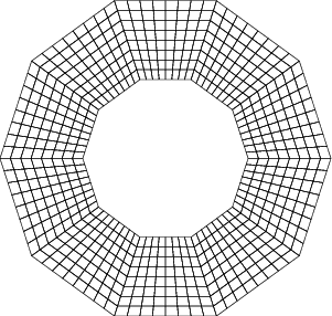
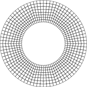
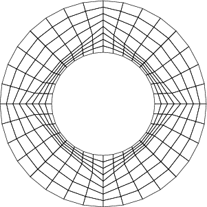
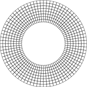
Figure 1: Illustration of the importance of taking geometry into account when refining meshes. Starting from a discretization of an annulus that contains ten coarse cells, we choose new points either ignoring the geometry description, i.e., computing the location of a new vertex by simply averaging the locations of the surrounding points (left), or choosing new points on boundary edges so that they have the correct radius from the origin, and new points of interior edges and cells as the Cartesian mean of the surrounding vertices (second from left). The latter procedure works well when the number of coarse elements is sufficient to resolve the geometry, but leaves some kinks in the grids, where one is still able to identify the original ten coarse cells. However, it may lead to very distorted grids if the coarse mesh is not fine enough, e.g., if the coarse mesh consisted of only four cells (second from right). The ideal case (right) is independent of the number of coarse cells that one may start with, and it exploits full knowledge of the underlying geometry. In this case, this is done by choosing all new points on edges and cells so that they average the radius and angle of the adjacent points.

In all of these cases, the new point on edges, faces, and cells can clearly be satisfied with the new point primitive of Section 2. (The different meshes shown in Fig. 1 then simply correspond to different ways of implementing the primitive.) In the case of isotropic refinement of edges, one needs to call the primitive with the two existing points and equal weights $w_{1}=w_{2}=\frac{1}{2}$. For the new point at the center of a quadrilateral, we first compute the new points on the edges, and then call the new point primitive for the new center point with the 8 surrounding points (the four pre-existing vertices of the quadrilateral plus the four new points on the now split edges). Assigning the existing vertices a weight of $-1/4$ and the new edge centers a weight $1/2$ leads to high-quality meshes, as opposed to putting equal weights on all points. These weights correspond to the evaluation with a transfinite interpolation [21] in the center of the edges. Similarly, for hexahedra, we call the new point primitive with the 8 existing vertices, the 12 new edge points, and the 6 new face centers, with weights $1/8$, $-1/4$, and $1/2$, respectively. Similar considerations can also be applied to triangles and tetrahedra.

3.2 Polynomial mappings

Many finite element codes use “iso-parametric” mappings in which cells consist of the area of the reference cell (e.g., the unit square) mapped by a polynomial mapping of degree equal to that of the finite element in use. (One may of course also use lower, “sub-parametric”, or even higher order, “super-parametric”, mappings.)

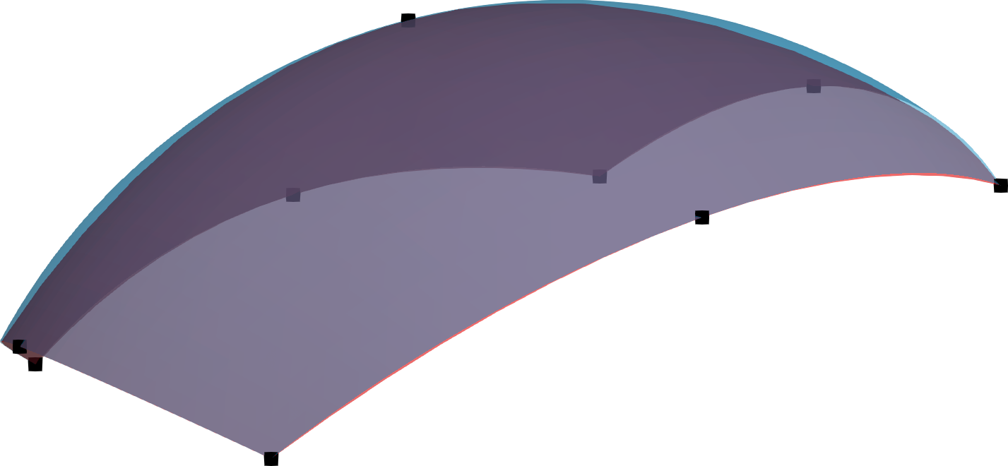
Figure 2: Illustration of biquadratic mapping of a quadrilateral (shown in red) onto the surface of a sixth of a sphere (blue), with interpolation nodes represented as black squares.

When using quadratic or higher order mappings, cells are bounded by polynomial curves or surfaces. In general, for quadrilaterals and hexahedra, a cell $K$ is defined by

$$K =\left\{\mathbf{x}\in{\mathbb{R}}^{d}:\mathbf{x}=\mathbf{F}_{K}(\mathbf{\hat{x}})=\sum_{i}\mathbf{v}_{i}\varphi_{i}(\mathbf{\hat{x}}),\quad\mathbf{\hat{x}}\in\hat{K}=[0,1]^{d}\right\}.$$ (2)

Here, $\varphi_{i}$ are the usual $d$-linear, $d$-quadratic, or higher order shape functions, and $\mathbf{v}_{i}$ are the $(p+1)^{d}$ support points of cell $K$ when working with mappings of degree $p$. (Similar constructions apply to triangles and tetrahedra.)

For $p=1$, i.e., the bi-/trilinear mappings, the support points are simply the vertices of the cell, for which we know that they are already part of the manifold, whose locations are fixed, and which are generally provided as part of the mesh description. On the other hand, for higher order mappings, we need to evaluate the locations of these support points between vertices. For example, for cubic mappings with equidistant support points, one needs these points at relative distances of 1/3 and 2/3 along each edge. This is easily done using the new point primitive, using the two vertices at the end of the edge as existing points, and weights $w_{1}=2/3,w_{2}=1/3$ for the first support point, and reversed weights for the second. Following the computation of edge support points, we proceed with the evaluation of support point locations inside each face using the already computed points at the vertices and on the edges as pre-existing points; finally, we compute locations for points inside cells. The weights within the entities might again be derived from transfinite interpolation [21], propagating the information from surrounding edges into the interior. Figure 2 illustrates the construction of such an approximate, polynomial representation of a part of a sphere. The support points for the mapping that are not existing vertices are generated using the new point primitive; consequently, they lie exactly on the curved (spherical) manifold, whereas there is a (small) gap between the polynomial approximation and the original sphere everywhere else.

All operations outlined in the previous paragraph only require the first of our two primitives. In Section 3.6, we analyze the requirements for implementing $C^{1}$-mappings that are needed in certain finite element applications.

3.3 Computing the Jacobian of a mapping

The computation of integrals in the finite element method generally involves the transformation $\mathbf{F}_{K}:\hat{K}\mapsto K$ from the reference cell $\hat{K}$ to the concrete cell $K$. The transformation of the integrand then implies that we need the “Jacobian” $J_{K}=\hat{\nabla}\mathbf{F}_{K}(\mathbf{\hat{x}})$ or its inverse for all vector quantities, and the determinant, $\text{det}(J_{K})$, as an additional weight factor. The Jacobian matrix $J_{K}$ is also necessary when using a Newton iteration to find the reference coordinates $\mathbf{\hat{x}}=\mathbf{F}^{-1}_{K}(\mathbf{x})$ that correspond to a given point $x$; this operation is key in particle-in-cell methods and methods based on characteristics. In the following, let us assume that $\mathbf{F}_{K}$ maps to the “true” domain of interest, not a polynomial approximation of it; we will comment on the latter case at the end of the section.

The construction of the matrix $J_{K}(\mathbf{\hat{x}})$ at a specific quadrature point $\mathbf{\hat{x}}_{0}$ given in reference coordinates uses an algorithm that first builds a basis for the tangent space at $\mathbf{x}_{0}=\mathbf{F}_{K}(\mathbf{\hat{x}}_{0})$. There are of course many bases for this tangent space, but we choose the one whose basis vectors are the images of unit vectors $\mathbf{\hat{e}}_{i}$ centered at $\mathbf{\hat{x}}_{0}$ as the images of these vectors will correspond to the partial derivatives $\frac{\partial}{\partial\hat{x}_{i}}\mathbf{F}(\mathbf{\hat{x}}_{0})$ and consequently form the columns of $J$. The algorithm proceeds in three steps:

1. Use the new point primitive with arguments given by the vertices of the concrete cell, and weights equal to the reference coordinates of $\mathbf{\hat{x}}_{0}$, to obtain the image $\mathbf{x}_{0}\in K$ of the point $\mathbf{\hat{x}}_{0}\in\hat{K}$;

2. Select $d$ points $\{\mathbf{\hat{x}}_{i}\}_{i=1}^{d}$ in the reference cell $\hat{K}$, aligned with the $i$th reference coordinate axis, and compute their images in $K$ using again the new point primitive with arguments given by the vertices of the cell $K$, and weights equal to the coordinates of the points $\mathbf{\hat{x}}_{i}$;

3. Call the tangent vector primitive $d$ times, with arguments $(\mathbf{x}_{0},\mathbf{x}_{i})$, divide the result by $L_{i}=\mathbf{e}_{i}\cdot(\mathbf{\hat{x}}_{i}-\mathbf{\hat{x}}_{0})=(\mathbf{\hat{x}}_{i}-\mathbf{\hat{x}}_{0})_{i}$, to obtain tangent vectors $\mathbf{t}_{i}$.

These vectors $\mathbf{t}_{i}$ form a basis of the tangent space (though they may neither be orthogonal nor normalized) and are then arranged to form the columns of $J_{K}(\mathbf{\hat{x}}_{0})$.

While one might in principle choose the points $\mathbf{\hat{x}}_{i}$ arbitrary in either $\pm\mathbf{\hat{e}}_{i}$ from $\mathbf{\hat{x}}_{0}$, in practice one wants to choose them as far away from $\mathbf{\hat{x}}_{0}$ as possible in the reference cell to obtain a well conditioned algorithm (see Fig. 3).

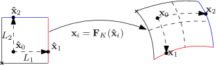
Figure 3: Computing the Jacobian of a mapping (at point $\mathbf{\hat{x}}_{0}$) using only the New Point and tangent vector primitives.

We note that in many cases, finite element codes do not use the exact mapping $\mathbf{F}_{K}$ from the reference cell $\hat{K}$ to a real cell $K$, but only a polynomial approximation (see Section 3.2). In those cases, it is of course trivial to compute the Jacobian matrix since it is simply the gradient of the mapping presented in (2), i.e.,

$$J_{K}(\mathbf{\hat{x}})=\sum_{i}\mathbf{v}_{i}\hat{\nabla}\varphi_{i}(\mathbf{\hat{x}}).$$

It is an exercise to show that the two methods indeed result in the same matrix for polynomial mappings.

3.4 Computing vectors normal to lower-dimensional manifolds

In our survey of existing uses of geometric information, we have found many instances where normal vectors to lower-dimensional surfaces embedded in higher dimensional space were required. These could either be the normals to $(d-1)$-dimensional faces of $d$-dimensional cells in $d$ space dimensions, or the normals to $d$-dimensional cells embedded in a $d^{\prime}$-dimensional space where $d^{\prime}>d$. Examples of such situations include the following:

• In the evaluation of boundary conditions: Across applications, there exist a wide variety of boundary conditions that require normal vectors. Among these are:

  • “No flux” boundary conditions on a vector velocity field $\mathbf{u}$ have the form $\mathbf{n}\cdot\mathbf{u}=0$. These require knowledge of the normal vector in the implementation because one typically imposes a constraint that determines one vector component in terms of the others, for example by evaluating the identity $u_{3}=-\frac{n_{1}u_{1}+n_{2}u_{2}}{n_{3}}$ at the support points of the shape functions.

  • In other cases, one may want to prescribe a particular tangential velocity in addition to no-flux conditions such as the one above. An example is the classical lid-driven cavity. In this case, one needs to also constrain the tangential part of the velocity, $(\mathbf{I}-\mathbf{n}\otimes\mathbf{n})\mathbf{u}$.

  • For hyperbolic equations, boundary conditions can only be imposed on inflow boundaries. Whether a part of the boundary is in- or outflow depends on the sign of $\mathbf{n}\cdot\mathbf{u}$ where $\mathbf{u}$ is either an externally prescribed velocity, or the solution of a previous time step or nonlinear iteration. Again, an explicit construction of the normal vector to the boundary is required.

  • In fluid-structure interaction problems, traction boundary conditions on the solid are common where the traction $T$ is given by $\mathbf{T}=p\mathbf{n}$ in terms of the fluid pressure $p$. It may also contain a viscous friction component $2\eta\varepsilon(\mathbf{u})\mathbf{n}$ where $\eta$ is the viscosity, $\mathbf{u}$ is the fluid velocity and $\varepsilon(\mathbf{u})$ its symmetric gradient.

  • In external scattering problems, one often only solves for the scattered, instead of the total field. The boundary conditions on the scatterer then involve the incident field $U_{\infty}$, and depending on the type of scatterer often contain terms of the form $U_{\infty}\mathbf{n}$.

• In discontinuous Galerkin (DG) discretizations: When using the discontinuous Galerkin method, one generally applies integration by parts on each element individually, resulting in face integrals of some quantities times the normal vector on the face. The numerical fluxes that weakly impose the continuity of solutions between the elements also often involve the normal vector [25]. One example are upwind formulations for hyperbolic equations, which consider the sign and magnitude of the quantity $\mathbf{n}\cdot\mathbf{u}$ where again $\mathbf{u}$ is a velocity field. Thus, the normal vector explicitly appears in the bilinear form that defines the discretization.

• In error estimation: Many error estimators for finite element discretizations contain terms that measure the “jump” from one cell to the next of the normal component of the gradient of the discrete solution. An example is the widely used “Kelly” error estimator for the Laplace equation [28, 19] that requires evaluating

  $$\eta_{K}=\left(\frac{h}{24}\int_{\partial K}\left[\mathbf{n}\cdot\nabla u_{h}\right]^{2}\;ds\right)^{1/2}$$

  for every cell $K$, where $[\cdot]$ denotes the jump across a cell interface. Similar terms appear in almost all other residual-based error estimates (see, for example, [1, 4, 5]).

• In boundary element methods: Boundary integral formulations hinge upon the availability of a fundamental solution for the PDE at hand; i.e., an (often singular) function $G$, such that the solution $u$ of a PDE at a point $\mathbf{x}\not\in\Gamma$ can be written as a function of the jump of the solution and of its normal derivative on the boundary $\Gamma$:

  $$u(\mathbf{x})+\int_{\Gamma}\mathbf{n}_{y}\cdot\nabla_{y}G(\mathbf{x}-\mathbf{y})[u(\mathbf{y})]d\Gamma_{y}=\int_{\Gamma}[\mathbf{n}_{y}\cdot\nabla_{y}u(\mathbf{y})]G(\mathbf{x}-\mathbf{y})d\Gamma_{y};$$

  see, for example, [42, 36, 20, 37].

• In postprocessing solutions: Computer simulations are typically done because we want to learn something from the solution, i.e., we need to evaluate or postprocess it after it is computed. Many of these postprocessing steps involve normal vectors at the boundary. For example, in Aspect alone, we evaluate the normal components of a flow field (or of the stress tensor) at the boundary to displace the boundary appropriately; we may compute the gravity field and its angle against actual surface topography to determine the direction of water and sediment transport; and we compute the normal component of the gradient of the temperature field to determine the heat flux through surfaces. Many other postprocessing applications come to mind that require the normal vector to the boundary. In other contexts, we require the normal vector to an embedded surface on which we solve equations, for example to assess the evolution of surfaces such as soap films or the membranes of cells.

In all of the cases above – typical of many complex finite element simulators – we require computing the normal vector to faces or cells. The construction of the normal vector $\mathbf{n}\in{\mathbb{R}}^{d}$ follows in essence the construction outlined in Section 3.3 for the Jacobian matrix, except that we map a lower-dimensional object (namely, a face of a cell) and can consequently only generate $d-1$ basis vectors. The algorithm then finds a set of $d-1$ tangent vectors $\mathbf{t}_{i}$ to the manifold (this involves using the tangent vector primitive), and we compute the normal vector using the wedge product,

$$\mathbf{n}=\pm\frac{\mathbf{t}_{1}\wedge\cdots\wedge\mathbf{t}_{d-1}}{\|\mathbf{t}_{1}\wedge\cdots\wedge\mathbf{t}_{d-1}\|}.$$ (3)

The sign is typically chosen so that $\mathbf{n}$ points outward from whatever object we are currently considering. The algorithm in Section 3.3 chooses a particular basis, that is, in particular neither orthogonal nor normalized. Neither is a problem here because the definition of $\mathbf{n}$ above is invariant under the choice of basis.

There are two situations that require additional thoughts:

• If one asks for the normals of faces of cells that are themselves embedded in a higher dimensional space: For example, a user code may require the jump of the normal derivative across the one-dimensional edges of two-dimensional cells, where the cells form a triangulation of a two-dimensional manifold embedded in three-dimensional space. In such a case, two orthogonal normals exist to the edge, and the one required in the code will likely be the one that is tangent to the manifold.

  In general, objects of dimensionality $d_{1}\leq d_{M}$ that are part of a triangulation of a manifold $M$ of dimension $d_{M}$ embedded in $d\geq d_{M}$ dimensional space allow for a system of $d-d_{1}$ mutually orthogonal normal vectors. In applications, we typically seek those that also lie in the $d_{M}$-dimensional tangent space to the manifold, leaving us with a choice of $d-d_{1}-(d-d_{M})$ mutually orthogonal normal vectors.

• In a similar case, we frequently seek the normal vector to a triangulated manifold of dimension $d_{M}$ embedded in a $d>d_{M}$ dimensional space. An application is to determine the direction of growth for the two-dimensional membrane surrounding a three-dimensional biological cell. In other applications, however, we consider embeddings in even higher dimensional spaces, $d>d_{M}+1$, in which case there is again a system of $d-d_{M}$ mutually orthogonal normal vectors that we will need to be able to compute.

In both of these situations, we can only compute a subset of the complete set of tangent vectors $\mathbf{t}_{i},i=1,\ldots,d-1$; the normal vector appropriate for the application can then generally be computed by providing the remaining tangent vectors from the context to complete the wedge product in (3).

3.5 Computing vectors tangent to lower-dimensional manifolds

There are also cases where computing tangent vectors to a boundary is necessary. For example, in electromagnetics applications, one often requires that the tangent component of the electric field vanishes. Mathematically, this is often expressed by requiring that $\mathbf{n}(\mathbf{x})\times\mathbf{E}(\mathbf{x})=0$ for all points $\mathbf{x}$ on the boundary of a domain, but actual applications generally implement this by requiring that $\mathbf{t}_{1}(\mathbf{x})\cdot\mathbf{E}(\mathbf{x})=\cdots=\mathbf{t}_{d-1}(\mathbf{x})\cdot\mathbf{E}(\mathbf{x})=0$, where the vectors $\mathbf{t}_{i}(\mathbf{x})$ form a complete (but otherwise arbitrary) basis of the tangent space to the boundary at the point $\mathbf{x}$. Each of these conditions is then imposed in the same way as the constraints corresponding to $\mathbf{n}\cdot\mathbf{u}=0$ in the previous section.

Since the concrete choice of basis vectors $\mathbf{t}_{i}$ is unimportant, we can again fall back to the construction discussed in Section 3.3 in order to impose $\mathbf{t}_{i}(\mathbf{x})\cdot\mathbf{E}(\mathbf{x})=0$. On the other hand, for stability purposes, it may also be convenient to orthonormalize these vectors, which is of course easily done using, for example, the Gram–Schmidt process.

3.6 $C^{1}$ mappings

As mentioned above, one frequently uses polynomial mappings from the reference cell $\hat{K}$ to each concrete cell $K$ of the mesh. In practice, this implies that curved boundaries are approximated by piecewise polynomials. The common construction of these mappings guarantees the continuity of the individual pieces of this boundary approximation at vertices, but the approximate boundary is not $C^{1}$ continuous at vertices (in 2d) and edges (in 3d). On the other hand, in some applications, it is desirable or necessary that curved boundaries are approximated with $C^{1}$ continuity.

One possible way to achieve this is to use cubic mappings, and to construct their face support points such that the mapping interpolates the actual manifold at the face vertices in such a way that the resulting mapping’s tangent space in vertices coincides with the tangent space of the underlying, original, curved boundary. If the boundary itself is continuously differentiable across face boundaries, this will guarantee that the resulting mapping is also continuously differentiable. To achieve this, we need to require that the cubic mapping $\mathbf{F}_{K}$ on cell $K$ satisfied the following conditions in each vertex $\mathbf{v}_{i},i=1,\ldots,2^{d-1}$ of the face:

$$\mathbf{F}_{K}(\mathbf{\hat{v}}_{i})=\mathbf{v}_{i},\qquad J_{K}(\mathbf{\hat{v}}_{i})\mathbf{\hat{n}}_{i}=\mathbf{n}_{i},$$ (4)

where the normals $\mathbf{n}_{i}$ are computed as in Section 3.4, while the normals $\mathbf{\hat{n}}_{i}$ are unit vectors perpendicular to the faces of the reference cell.

The above conditions can then be used to fix the locations of the (non-vertex) support points of the cubic mapping on the face, by providing $2^{d}$ conditions on the $2^{d}$ support points on the faces. (However, these non-vertex locations will, in general, not actually lie on the original boundary.) The remaining support points can be set using the new point primitive, as in Section 3.2, completing the information necessary for the construction of a cubic mapping $\mathbf{F}_{K}$.

4 Geometry specification formats

In order to understand how the two primitives can be implemented in common, industrial use cases, let us use this section to discuss the ways in which geometry information is typically available: namely, either in the form of combinations of simple geometries, or in the form of a collection of analytically known patches that together provide a boundary representation for the domain of interest.

4.1 Constructive Solid Geometry

In some cases, the shape of the computational domain admits an analytic representation for which it is straightforward to implement the primitives described in Section 2. For example, if the domain corresponds to a cube, a parallelogram, or a sphere, then it can be described in the language of differential geometry where each local portion of the domain (a “chart”) is the image of a Cartesian space under an analytically known “push-forward” operation. In such cases, the new point operation is easily represented by applying the “pull-back” to the surrounding points, averaging in the Cartesian domain, and “pushing forward” the resulting point. The tangent vector operation follows the same idea. We discuss these algorithms in more detail in Section 5.1.

It is straightforward to generalize this procedure for shapes that are further transformed from relatively simple original geometries – for example, when using a true topographic model of the Earth instead of a sphere; in those cases, the pull-back and push-forward operations are simply concatenations of the Cartesian-to-simple-geometry and simple-to-transformed-geometry operations.

A generalization of this approach is commonly known as “Constructive Solid Geometry” (CSG): Here, solids are expressed as as the union, intersection, or set difference of simpler solids (e.g., cubes, prisms, spheres, cylinders, cones, and toruses, possibly subject to transformations). An example involving boxes and cylinders is shown in Figure 4. The implementation of our primitives then requires keeping track of which part of the geometry one is on, and the primitives are implemented by falling back to the case of a single, analytically known geometry for which we have provided a description above.

. .

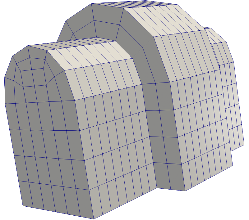
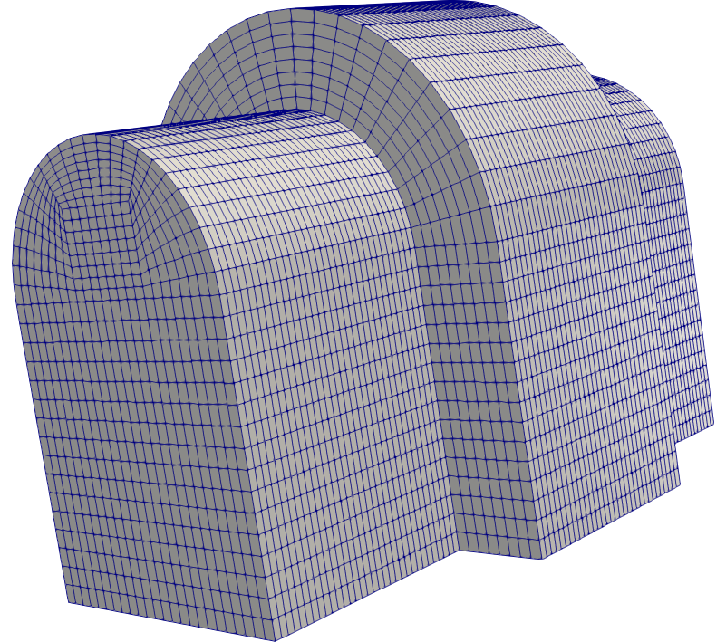
Figure 4: Example of geometry constructed using simple Constructive Solid Geometry primitives and shapes, taken from the deal.II tutorial program step-49 [24]. Left: Coarse mesh. Right: A refined mesh that uses the underlying geometry description of the domain’s pieces to place new vertices.

4.2 Boundary Representation Models

In the vast majority of industrial cases, domains are specified through a boundary representation model (B-REP or BREP), used to combine topological and geometrical information to provide a complete description of the boundary of the domain. A solid (or surface) is then represented as a collection of connected surface (or curve) elements: this set of $d-1$-dimensional surface(s), embedded into $d$-dimensional space, represents the boundaries of the domain.

There are two general ways in which these boundaries are often provided: (i) In CAD applications, curves and surfaces are generally parameterized as Non-Uniform Rational B-Splines (NURBS); (ii) The surface of the domain is given as a triangulated surface, often obtained from a point cloud derived from measurements on an actual object.

4.2.1 Boundaries represented through NURBS

Here, individual patches are defined as parametric surface patches that have an analytical representation. In three space dimensions, this representation is often provided by a mapping from a “reference domain” with coordinates $u,v$ to a NURBS surface. So, within each patch, one might think that all information associated with the primitive operation is easily obtained using this mapping from $u$-$v$ space to ${\mathbb{R}}^{3}$. In practice, however, this mapping may map equal areas in $u$-$v$ space to rather unequal areas on the surface in ${\mathbb{R}}^{3}$; one also encounters difficult issues if one needs to cross from one NURBS patch to another when evaluating our two primitives. We will therefore discuss the practical implementation of the primitives in Section 5 below, and for the moment simply state that the primitives can be implemented based on NURBS B-REPs.

Practical realizations need to read and properly interpret the content of CAD data structures. This is made possible through open source libraries such as OpenCASCADE [41], which provide tools for importing and interrogating vendor-neutral CAD file formats such as IGES and STEP [27, 33, 40].

4.2.2 Boundaries represented by triangulated point clouds

In many other cases, the boundary is described by points: a polygonal chain in 2d, or a triangulation in 3d. These are often used to represent the most topologically intricate domains, and are for instance used by software which extracts geometrical models from MRI images or 3d laser scans. Several CAD modeling tools can also export triangulated surfaces. A popular file format is STL, which originated in the stereolithography community but is now widely used in industrial continuum mechanics applications and 3D printer geometry specifications.

Despite their wide usage, triangulated surfaces also pose several problems in the implementation of suitable primitive operators. In principle, the primitives can locate new points and compute tangent vectors based on the planar surfaces associated with each triangle. However, there is typically no guarantee that the triangles form a closed surface – models may have holes or gaps in which a new point or a tangent vector cannot be identified. More importantly, in order to provide effective information to a finite element algorithm, the diameters of triangles must be significantly smaller than those of the finite element mesh: Only then will the triangulated surface appear smooth compared to the finite elements mesh. Such requirements lead in most situations to surfaces triangulated by extremely large numbers of elements, resulting in high storage costs and expensive computations to identify new points and tangent vectors as both require looping over the many triangular faces.

5 Possible implementations

Section 3 has shown that essentially all geometrical queries required in finite element codes can be implemented by only using the two operations described in Section 2. However, we have not discussed how these primitives can be implemented for the kinds of geometries one frequently encounters in simulations. Section 4 might have given some hints, but also outlined some of the difficulties. This section discusses common approaches.

It is important to note that the way this is done is not unique, and there are often different possible implementations of the primitives. For example, in Section 6 we will show results where $\mathbf{x}^{\ast}$ is chosen as the directional, orthogonal, or closest point projection onto a surface. These choices may result in meshes of different quality, but this is immaterial to the key point of this paper as they only affect how an oracle implements a query, not the kinds of queries it has to be able to answer.

5.1 Implementing primitives for analytically known charts

The simplest way to implement the two primitives is if we have direct and explicit access to an atlas that describes the actual manifold of which the domain is a part. We can then rely on the language and methods of differential geometry.

An atlas for a manifold $M$ of dimension $d$ is a collection of coordinate “charts” (also called coordinate patches, or local frames): homeomorphisms $\phi_{\alpha}$ from an open subset $U_{\alpha}$ of $M$ to an open subset $U_{\alpha}^{\ast}$ of the Euclidean space of dimension $d$, such that $\cup_{\alpha}U_{\alpha}=M$. By definition, the sets $U_{\alpha}$ and $U_{\alpha}^{\ast}$ are connected by push-forward and pull-back functions, $\phi_{\alpha}:U_{\alpha}^{\ast}\rightarrow U_{\alpha}\subseteq M$ and $\phi_{\alpha}^{-1}:U_{\alpha}\rightarrow U_{\alpha}^{\ast}$.

With these definitions, if a point $\mathbf{x}_{2}$ lies in the same set $U_{\alpha}$ of the point $\mathbf{x}_{1}$ (i.e., if they lie on the same chart), then the parametric line that connects them is the image of the straight line $\phi_{\alpha}^{-1}(\mathbf{x}_{1})+t\left(\phi_{\alpha}^{-1}(\mathbf{x}_{2})-\phi_{\alpha}^{-1}(\mathbf{x}_{1})\right)$ in $U_{\alpha}^{\ast}$ under $\phi_{\alpha}$, i.e.,

$$\mathbf{s}(t)=\phi_{\alpha}\left(\mathbf{x}_{1}^{\ast}+t\left[\mathbf{x}_{2}^{\ast}-\mathbf{x}_{1}^{\ast}\right]\right)=\phi_{\alpha}\left(\phi_{\alpha}^{-1}(\mathbf{x}_{1})+t\left[\phi_{\alpha}^{-1}(\mathbf{x}_{2})-\phi_{\alpha}^{-1}(\mathbf{x}_{1}\right]\right).$$

Therefore, when the push-forward and the pull-back are explicitly available, a straightforward implementation of the new point primitive with any number of points that belong to the same set $U_{\alpha}$ is given by the following

$$\mathbf{x}^{\ast}(\mathbf{x}_{1},\ldots,\mathbf{x}_{N},w_{1},\ldots,w_{N})=\phi_{\alpha}\left(\sum_{n=1}^{N}w_{n}\phi_{\alpha}^{-1}(\mathbf{x}_{n})\right).$$

That is, we simply take the weighted average of the pulled back points $\phi_{\alpha}^{-1}(\mathbf{x}_{n})$ and push the average forward.

Furthermore, the tangent vector primitive is also easy to compute using the formula

$$\mathbf{t}(\mathbf{x}_{1},\mathbf{x}_{2})=\nabla^{\ast}\phi_{\alpha}\left(\mathbf{x}_{1}^{\ast}\right)\left[\mathbf{x}_{2}^{\ast}-\mathbf{x}_{1}^{\ast}\right]=\nabla^{\ast}\phi_{\alpha}\left(\phi_{\alpha}^{-1}(\mathbf{x}_{1})\right)\left[\phi_{\alpha}^{-1}(\mathbf{x}_{2})-\phi_{\alpha}^{-1}(\mathbf{x}_{1})\right],$$

where $\nabla^{\ast}\phi_{\alpha}(\mathbf{x}^{\ast})$ is the gradient of the push-forward function for the chart around $\mathbf{x}^{\ast}$.

5.2 Implementing primitives based on geodesics

The formulas available for analytically known charts suggest that the quality of the implementation depends on whether or not $\phi_{\alpha}$ is constructed in a “reasonable” way. In order to produce the least distorted grids upon refinement, one would like $\phi_{\alpha}$ to map straight lines in $U_{\alpha}^{\ast}$ to geodesic paths on $M$. In general, the construction of explicit geodesics is only possible on simple manifolds, and even there, subtle problems lurk.

For example, it is tempting to construct the new point primitive with two points directly in terms of geodesics. If we parameterize a geodesic that connects $\mathbf{x}_{1},\mathbf{x}_{2}$ as $\mathbf{s}(t)$ so that $\mathbf{x}_{1}=\mathbf{s}(0)$, $\mathbf{x}_{2}=\mathbf{s}(1)$, and assume that $\mathbf{s}(t)$ moves at constant speed (as measured by the metric), then this suggests the following implementation: given $\mathbf{x}_{1},\mathbf{x}_{2}$ and weights $w_{1},w_{2}=1-w_{1}$, define

$$\mathbf{x}^{\ast}\left(\mathbf{x}_{1},\mathbf{x}_{2},w_{1},1-w_{1}\right)=\mathbf{s}(w_{1}),$$

Similarly, we can construct the tangent vector primitive for two points $\mathbf{x}_{1},\mathbf{x}_{2}$ connected by the geodesic $\mathbf{s}(t)$ as

$$\mathbf{t}=\mathbf{s}^{\prime}(0).$$

While reasonable, this construction solely based on geodesics is only useful if geodesics connecting two points are unique. In general, this requires that the points are “close together” in some sense – which in the finite element context means that the mesh is already sufficiently fine since we generally call the primitives with points that are located on the same cell. Moreover, its generalization to more than two points is not at all trivial. Indeed, consider a recursive implementation for the new point primitive with more than two points: Given $\mathbf{x}_{1},\ldots,\mathbf{x}_{N}$, $w_{1},\ldots,w_{N}$, $N>2$, define

$$\mathbf{x}^{\ast}\left(\mathbf{x}_{1},\mathbf{x}_{2},\ldots,\mathbf{x}_{N},w_{1},w_{2},\ldots,w_{N}\right)=\mathbf{x}^{\ast}\left(\mathbf{s}_{12}\left(\frac{w_{1}}{w_{1}+w_{2}}\right),\mathbf{x}_{3}\ldots,\mathbf{x}_{N},w_{1}+w_{2},w_{3},\ldots,w_{N}\right)$$

where, without loss of generality, we have assumed that point $\mathbf{x}_{1}$ has a nonzero weight $w_{1}>0$, and where $\mathbf{s}_{12}(t)$ is the (presumed unique) geodesic connecting $\mathbf{x}_{1},\mathbf{x}_{2}$. It is not difficult to show that, in general, the algorithm above depends on the order in which points and weights are given. Furthermore, the operation is not associative in the following sense: Consider, for example, a situation with the four vertices of a quadrilateral cell and four equal weights $w_{i}=\tfrac{1}{4}$. Using the recursive definition of $\mathbf{x}^{\ast}$ above, one can compute

$$\mathbf{x}_{1234} =\mathbf{x}^{\ast}(\mathbf{x}_{1},\mathbf{x}_{2},\mathbf{x}_{3},\mathbf{x}_{4},\tfrac{1}{4},\tfrac{1}{4},\tfrac{1}{4},\tfrac{1}{4})$$

$$\tilde{\mathbf{x}}_{1234} =\mathbf{x}^{\ast}(\mathbf{x}_{12},\mathbf{x}_{34},\tfrac{1}{2},\tfrac{1}{2})\quad\text{with }\mathbf{x}_{12}=\mathbf{x}^{\ast}(\mathbf{x}_{1},\mathbf{x}_{2},\tfrac{1}{2},\tfrac{1}{2})\text{ and }\mathbf{x}_{34}=\mathbf{x}^{\ast}(\mathbf{x}_{3},\mathbf{x}_{4},\tfrac{1}{2},\tfrac{1}{2}).$$

In general, $\tilde{\mathbf{x}}_{1234}\neq\mathbf{x}_{1234}$, contrary to expectation. However, both are “reasonable” intermediate points, and it is not clear which option to prefer. This ambiguity suggests that this may not be a useful algorithm.

A commutative alternative algorithm is to take the average over all possible permutations of the pairs $(\mathbf{x}_{i},w_{i})$:

$$\mathbf{x}^{\ast}\left(\mathbf{x}_{1},\mathbf{x}_{2},\ldots,\mathbf{x}_{N},w_{1},w_{2},\ldots,w_{N}\right):=\frac{1}{N!}\sum_{k=1}^{N!}\mathbf{x}^{\ast}_{\text{recursive}}(S_{k}(\mathbf{x},w)),$$

where $S_{k}(\mathbf{x},w)$ is the $k$th permutation of the $N$ pairs $\{\mathbf{x}_{i},w_{i}\}_{i=1}^{N}$ and $\mathbf{x}^{\ast}_{\text{recursive}}$ is the recursive implementation from before. Of course, such an algorithm is, in general, quite expensive given that, for example, one already has to consider $8!=40,320$ permutations for finding the point that interpolates the vertices of a hexahedron.

There is also the issue of how exactly one finds the appropriate point on a geodesic. In many practical applications, a geodesic is easy to describe geometrically, but parameterizing it is more complicated; in those cases, one may be tempted to first average the input points in the ambient space and only then project onto the geodesic – avoiding to provide the geodesic with an arc-length that can be used to find intermediate points. But this yields yet another complication: Consider, for example,

$$\mathbf{x}_{12}=\mathbf{x}^{\ast}(\mathbf{x}_{1},\mathbf{x}_{2},\tfrac{3}{4},\tfrac{1}{4}),\qquad\qquad\qquad\tilde{\mathbf{x}}_{12}=\mathbf{x}^{\ast}\big{(}\mathbf{x}_{1},\mathbf{x}^{\ast}(\mathbf{x}_{1},\mathbf{x}_{2},\tfrac{1}{2},\tfrac{1}{2}),\tfrac{1}{2},\tfrac{1}{2}\big{)}.$$ (5)

The first formula represents the point at $1/4$ of the geodesic between $\mathbf{x}_{1}$ and $\mathbf{x}_{2}$, whereas the second first computes the mid point $\mathbf{x}_{\text{m}}$ between $\mathbf{x}_{1}$ and $\mathbf{x}_{2}$, and then the mid point between $\mathbf{x}_{1}$ and $\mathbf{x}_{\text{m}}$. Unfortunately, the definition of $\mathbf{x}^{\ast}$ based on the projection onto geodesics does not always provide that the two points are the same. It is not difficult to construct examples where this ambiguity has concrete, detrimental effects on the accuracy of finite element operations. For example, when interpolating a finite element solution from a parent cell $K$ (say, the image of the interval $(0,1)$ under a transformation $\Phi_{K}$) to its first child $K^{\text{child 0}}$ (the image of $(0,\tfrac{1}{2})$ under $\Phi_{K}$), then we will want that the point with reference coordinates $\xi$ on the child cell equals the point with reference coordinates $\xi/2$ on the parent cell when evaluating finite element shape functions. This can, in general, be ensured for $d=1$, but not for $d\geq 2$: There, the construction above (where we have considered $\xi=\tfrac{1}{2}$) shows that that the two points may be different, and one can observe that this affects the convergence order of some algorithms.

Table 1: Effect on the numerical error for interpolation between two successive mesh levels in a spherical shell, using a spherical manifold with spherical averages as the new point oracle.

Polynomial degree $p=4$				Polynomial degree $p=7$
$n_{\text{DoF,coarse}}$	error coarse	error after refine		$n_{\text{DoF,coarse}}$	error coarse	error after refine
490	$7.25\cdot 10^{-2}$	$6.92\cdot 10^{-2}$		2,368	$2.92\cdot 10^{-3}$	$9.70\cdot 10^{-3}$
3,474	$2.42\cdot 10^{-3}$	$4.16\cdot 10^{-3}$		17,670	$1.16\cdot 10^{-5}$	$3.28\cdot 10^{-3}$
26,146	$1.05\cdot 10^{-4}$	$2.74\cdot 10^{-4}$		136,474	$6.68\cdot 10^{-8}$	$2.56\cdot 10^{-4}$
202,818	$3.38\cdot 10^{-6}$	$1.66\cdot 10^{-5}$		1,072,626	$2.21\cdot 10^{-10}$	$1.62\cdot 10^{-5}$
1,597,570	$1.06\cdot 10^{-7}$	$1.02\cdot 10^{-6}$		8,505,058	$8.71\cdot 10^{-13}$	$1.02\cdot 10^{-6}$

For the sphere, where the construction of geodesics is trivial, [11] provides exhaustive discussions that show that various possibilities for evaluating $\mathbf{x}^{\ast}$ with three or more input points yield results that differ by quantities of order ${\mathcal{O}}(D^{4})$ where $D$ is a measure of the distance between the input points. Table 1 shows the result of an experiment in this vein: Given a subdivision of a spherical shell in ${\mathbb{R}}^{3}$ with inner and outer radii $0.5$ and $1.0$ into hexahedra, we define a finite element field $u_{h}$ of polynomial degree $p$ whose nodal values are chosen so that $u_{h}$ interpolates a known smooth function $u$. We show $\|u-u_{h}\|_{L_{2}}$ in the columns labeled “error coarse” for $p=4$ and $p=7$ in the table. We can observe the error decrease approximately as ${\mathcal{O}}(h^{p+1})$ as the mesh is chosen finer and finer, as expected.

For each of these meshes, we then perform one isotropic refinement and interpolate $u_{h}$ onto $u_{h/2}$ by using the embedding of the two spaces on the reference cell (rather than interpolating $u$ onto $u_{h/2}$). Of course, one would expect the difference $\|u-u_{h/2}\|$ to be the same as before since we expect that $u_{h/2}=u_{h}$. But this equality assumes that the support points of the child cells of size $h/2$ (when computed using the interpolation between the vertices of the child cell) are located at the positions where one would have expected them to be when interpolating the (child cell’s) support points using the vertices of the parent cell. Given considerations such as in (5), this is not the case, and due to this difference, the error $\|u-u_{h/2}\|$ is actually substantially larger than $\|u-u_{h}\|$ and, instead of the optimal convergence rate $\mathcal{O}(h^{p+1})$, only converges as $\mathcal{O}(h^{4})$.

These, and the examples below, demonstrate that the implementation of $\mathbf{x}^{\ast}$ is not obvious even in situations where we have reasonable pull-back and push-forward operations. Indeed, the message of this section is that there are no obvious solutions, but a variety of approaches that yield reasonable implementations good enough for many cases – the fact that they might affect convergence rates when used without a deeper understanding notwithstanding.

There are also cases where not even the definition of pull-back and push-forward functions is easily possible. For example, if the points $\mathbf{x}_{n}$ do not fall within the same set $U_{\alpha}$, it may not be possible to construct a single chart parameterized by $\phi_{\alpha}$ that encompasses all points $\mathbf{x}_{n}$. This may lead to unpleasant ambiguities, such as in the case of periodic domains (see Appendix B) or where only piece-wise descriptions of the geometry are available (e.g., CAD geometries via collections of NURBS patches).

5.3 Implementing primitives based on projections onto CAD geometries

For CAD geometries, any two points may fall across two different (non-overlapping) NURBS patches $U_{\alpha}$ and $U_{\beta}$. But there are more difficulties that make it difficult to implement the primitives based on pull back/push forward approaches:

1. NURBS patches do not always satisfy the requirements of a chart in the topological sense, i.e., they may be non-invertible in some points, and they may be non-smooth ( i.e., contain corners and edges within a single $U_{\alpha}$).

2. The metric $\phi_{\alpha}$ that results from mapping $u$-$v$ space to a NURBS patch $U_{\alpha}$ may be ill-formed: Its derivative may be close to zero near some points, and large at others – equally spaced points in $u$-$v$ space (or points $\mathbf{x}^{\ast}(\mathbf{x}_{1},\mathbf{x}_{2};w_{1},(1-w_{1}))$ for equally spaced values of $w_{1}$) would then be mapped to highly unevenly spaced points.

3. The evaluation of the pull-back $\phi_{\alpha}^{-1}(\mathbf{x})$ is computationally very expensive for NURBS patches.

As a consequence, useful implementations of our primitives will not be based on the concepts of differential geometry, but will rather be projection-based. Indeed, a possible implementation of the new point primitive for (multi-patch) CAD-based geometries is provided by the following algorithm: Given $\mathbf{x}_{1},\ldots,\mathbf{x}_{N}$, $w_{1},\ldots,w_{N}$, $N\geq 2$, define

$$\mathbf{x}^{\ast}\left(\mathbf{x}_{1},\mathbf{x}_{2},\ldots,\mathbf{x}_{N},w_{1},w_{2},\ldots,w_{N}\right)=P_{\text{CAD}}\left(\sum_{n=1}^{N}w_{n}\mathbf{x}_{n}\right),$$

where $P_{\text{CAD}}(\mathbf{x})$ is a projection of the point $\mathbf{x}$ onto the CAD surface (or curve). We will discuss various choices for the projection operator $P_{\text{CAD}}$ below, given that the choice will influence the quality of the result. We note that projection-based strategies have been proposed in [18] and are used in a basic variant for a high-order finite element code in [30]. Many CAD programs, and specifically the OpenCASCADE library [41] that we use for the examples shown here, implement all of the operations necessary for the three approaches to implementing a projection discussed below.

5.3.1 Projection in a fixed direction

The cheapest way to compute a projection is if the direction of the projection $\mathbf{d}\in{\mathbb{R}}^{d}$ is known a priori – for example, because we know that the surface in question has only minor variation from being horizontal. In that case, one might choose

$$\mathbf{x}^{\ast}\left(\mathbf{x}_{1},\mathbf{x}_{2},\ldots,\mathbf{x}_{N},w_{1},w_{2},\ldots,w_{N}\right)=I_{\text{CAD}}\left(\sum_{n=1}^{N}w_{n}\mathbf{x}_{n},\mathbf{d}\right),$$

where $I_{\text{CAD}}(\mathbf{x},\mathbf{d})$ is the intersection of the line $\mathbf{s}(t)=\mathbf{x}+s\mathbf{d}$ and the CAD surface (or curve). In other words, we first average all points $\mathbf{x}_{i}$ and then move the average back onto the surface along direction $\mathbf{d}$.

5.3.2 Projections taking into account the normal vector

In more general situations, however, choosing a projection direction a priori is not possible. Rather, one needs to take into account the geometry of the CAD surface in the vicinity of the point to be projected, for example by considering the normal vectors to either the existing mesh, or to the surface.

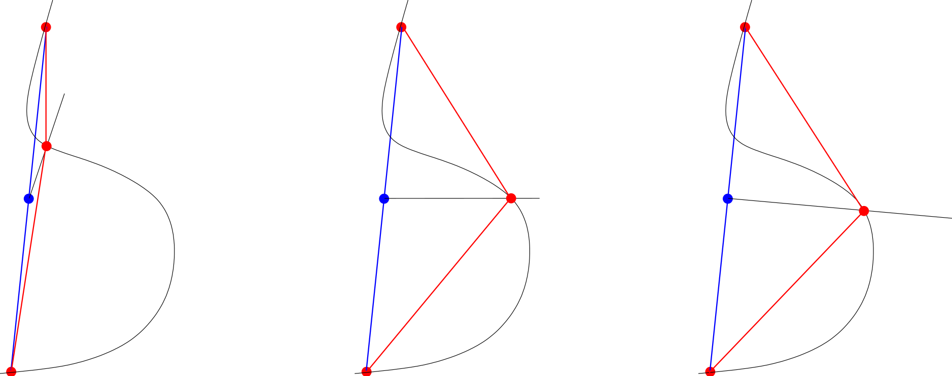
Figure 5: Comparison of three different implementations of the new point primitive for CAD geometries. The red end points (coarse vertices) of the blue line (coarse cell) form the inputs $\mathbf{x}_{1},\mathbf{x}_{2}$ for which we want to use the new point primitive to find a new mid-point (i.e., $w_{1}=w_{2}=\tfrac{1}{2}$). The blue point is the average of the original vertices to be projected onto the curved geometry. Left: Projection normal to the geometry. Center: Projection in a direction chosen a priori. Right: Projection normal to coarse mesh.

The first of these options (shown in the right panel of 5) would use the following implementation:

$$\mathbf{x}^{\ast}\left(\mathbf{x}_{1},\mathbf{x}_{2},\ldots,\mathbf{x}_{N},w_{1},w_{2},\ldots,w_{N}\right)=I_{\text{CAD}}\left(\sum_{n=1}^{N}w_{n}\mathbf{x}_{n},\mathbf{n}\right),$$

where the direction $\mathbf{n}$ is now (an approximation) to the normal vector of the area identified by the points $\mathbf{x}_{n}$. $\mathbf{n}$ is clearly defined if one only has $d$ input points in $d$ dimensional space; if there are more points – e.g., the four vertices of a face of a hexahedron in 3d – then one will want to define some useful approximate vector, e.g., the vector normal to the least squares plane that approximates the point locations. As is clear from the figure, if this implementation is chosen for mesh refinement, one generally ends up with refined meshes with cells of rather uniform sizes.

To use this approach, one needs to have at least $d$ input points in $d$ dimensions in order to define a unique direction normal to the existing points. But we also need to be able to use the new point primitive when finding a new midpoint for an edge in 3d. Thus, we need an additional condition to identify a unique direction among all of those perpendicular to the line connecting the existing edge end points. We do this by averaging the CAD surface normal at the vertices of the edge (both of which we know are on the surface), and then projecting it onto the edge’s axial plane.

An alternative, often implemented in CAD tools but expensive to evaluate, is to use a direction vector $\mathbf{n}$ that is perpendicular to the actual geometry, rather than to the current mesh. This is shown in the left panel of Fig. 5 and may lead to child cells of different size. Ultimately, however, once the mesh is already a good approximation to a surface, both of the approaches mentioned here will yield very similar results.

5.3.3 Implementing the tangent vector primitive for CAD surfaces

In all three of the project-based cases above, the implementation of the tangent vector primitive may be constructed using a finite differences approximation as already mentioned in Remark 2. A more accurate approach pushes forward the tangent vector at the pulled-back point.

5.4 Extending boundary representations into volumes

The previous sections only dealt with finding points and tangent vectors on a lower-dimensional surface, given points already on that surface. On the other hand, finite element codes typically use volume meshes for which the CAD geometry only provides information about the boundary. Thus, one still needs a way to extend this information into the interior of the domain – the importance of this step is apparent by looking at Fig. 1.

A general mechanism for this task is based on transfinite interpolation [21]. A transfinite interpolation maps points from some reference space $\hat{\mathbf{x}}\in\hat{K}=[0,1]^{d}$ to points in real space $\mathbf{x}$ by a weighted sum of information on the geometry of the faces of the image of $\hat{K}$. For example, for a quadrilateral in two dimensions

$$\mathbf{x}(\hat{x}_{1},\hat{x}_{2})=(1-\hat{x}_{2})\mathbf{c}_{0}(\hat{x}_{1})+\hat{x}_{2}\mathbf{c}_{1}(\hat{x}_{1})+(1-\hat{x}_{1})\mathbf{c}_{2}(\hat{x}_{2})+\hat{x}_{1}\mathbf{c}_{3}(\hat{x}_{2})\\ -\left[(1-\hat{x}_{1})(1-\hat{x}_{2})\mathbf{x}_{0}+\hat{x}_{1}(1-\hat{x}_{2})\mathbf{x}_{1}+(1-\hat{x}_{1})\hat{x}_{2}\mathbf{x}_{2}+\hat{x}_{1}\hat{x}_{2}\mathbf{x}_{3}\right].$$

Here, $\bf c_{0}(s),\bf c_{1}(s),\bf c_{2}(s),\bf c_{3}(s)$ are the four parameterized curves describing the geometry of the edges of the deformed quadrilateral and $\bf x_{0},\bf x_{1},\bf x_{2},\bf x_{3}$ are the four vertices. The evaluation on each edge is done via the new point primitive $\mathbf{x}^{\ast}$, i.e., $\mathbf{c}_{0}(s)=\mathbf{x}^{\ast}(\mathbf{x}_{0},\mathbf{x}_{1},1-s,s)$ and similarly for the other curves. If an edge is straight, then $\bf c_{0}(s)=(1-s)\mathbf{x}_{0}+s\mathbf{x}_{1}$. Similar formulas extend to the three-dimensional case. The important point is that transfinite mappings exactly respect the geometry of the boundary, while extending it smoothly into the interior of the domain.

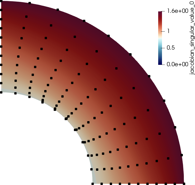
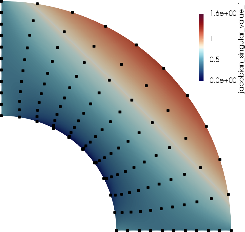
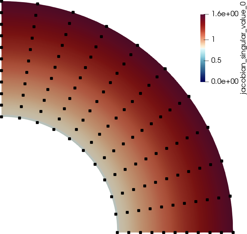
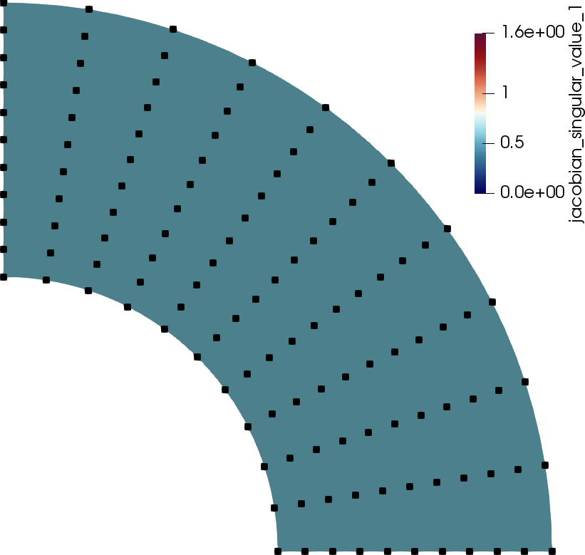
Figure 6: Illustration of the two singular values of $J_{K}=\hat{\nabla}\mathbf{F}_{K}(\mathbf{\hat{x}})$ for a quarter of a two-dimensional annulus; here, $\mathbf{F}_{K}$ is a polynomial mapping of a single element of degree 10. The ratio of the largest over the smallest singular value appears in the interpolation error estimate of the Bramble–Hilbert lemma, and consequently also in all error estimates for partial differential equations. Left two panels: Maximal and minimal singular value for point placement based on Laplace smoothing. Right two panels: Maximal and minimal singular value for point placement using a transfinite interpolation. (See the main text for interpretation.) The figures also include the positions of $11^{2}$ points equidistantly placed onto the reference cell and then mapped by $\mathbf{F}_{K}$ to the cell $K$ shown here, to illustrate the distortion.

We visualize this approach using higher order mappings. We recall that finite element error estimates on curved cells depend on the product of a Sobolev norm of higher order derivatives of $\mathbf{F}_{K}$ times a norm of the derivatives of $\mathbf{F}_{K}^{-1}$ (see, e.g., [14] or [43, Sec. 3.3]), which we visualize by the ratio between the largest and smallest singular value of $J_{K}$. Figure 6 compares the singular values for two variants of computing the interior points from the surrounding 11 points per line, i.e., a mapping of polynomial degree 10, on a quarter of an annulus with inner and outer radii $0.5$ and $1$, respectively. If the weights for the interior points are derived from solving a Laplace equation in the reference coordinates, the representations becomes distored, as is visible from the point distributions. This leads to a ratio of up to 100 between the largest and smallest singular value of the Jacobian $J_{K}=\hat{\nabla}\mathbf{F}_{K}(\mathbf{\hat{x}})$, and theory suggests a break-down of convergence; in experiments, $L_{2}$ errors of the solution to the Laplacian converge at best at third order. Conversely, using weights from transfinite interpolation results in a minimal singular value of 0.5 throughout the whole domain in this example. The resulting point distribution with transfinite interpolation in this particular example is equivalent to an explicit polar description of the whole domain, but applicable to generic situations with optimal convergence if the coarse cells are valid. We note that these and similar concepts are established in high-order meshing, but with algorithms typically acting on the points of associated polynomial descriptions, see e.g. [44, 26, 39, 35, 16, 30, 34] and references therein, rather than the abstract definition used here.

We associate the transfinite interpolation with the the initial (“coarse”) mesh of a finite element computation: each coarse mesh cell is used to define the reference coordinate system $\hat{x}$, and this is kept fixed even after many generations of descendants. Interior edges between refined cells are then curved, ensuring high mesh quality, assuming that the initial coarse cells reasonably approximate the geometry. Some of the computations involved in this process can be expensive, and we have therefore implemented caches that mitigate the cost for the case of polynomial mappings.

6 Application examples

In the following, let us illustrate the ideas of the previous sections using concrete applications. In particular, we will show how the implementation of the two primitives affects the meshes one obtains for an industrial application (Section 6.1) and an example of how one can choose metrics to generate graded meshes. In addition, let us refer to Fig. 1 for an illustration of the transfinite interpolation approach for extending surface descriptions to volume interiors.

6.1 Surface meshes described by CAD geometries

As discussed in detail in previous sections, CAD surfaces consist of patches that are the images of simpler domains in a two-dimensional $u$-$v$ space. Let us first consider a case where the geometry is described by a single, albeit rather complex, patch. The issue in even this simplified case is that a patch can be parameterized in many different ways, not all of which imply a more or less constant metric. Thus, it is unwise – although very common – to generate a mesh in $u$-$v$ space to obtain the corresponding three-dimensional surface grid, even though this of course has the advantage of generating nodes directly on the desired surface. Yet, the resulting mesh will generally have cells of rather unequal sizes and may show other severe deformations.

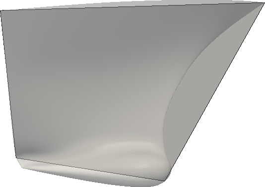
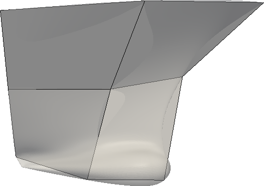
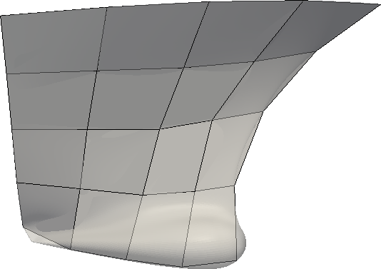
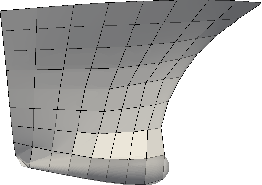
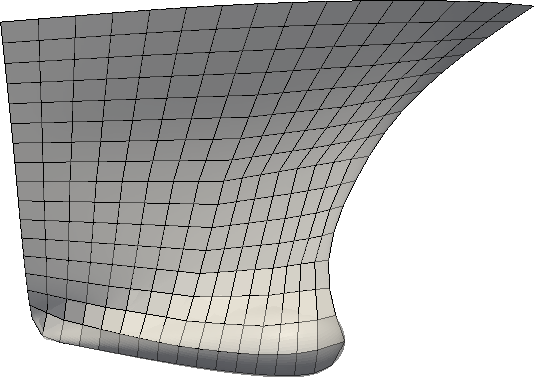
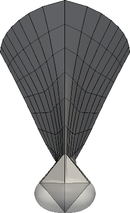
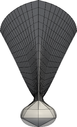
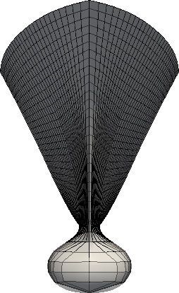
Figure 7: Directional projection strategy with a horizontal direction of projection perpendicular to the axis of symmetry. The first two rows show side views of the coarse grid and grids obtained from five successive refinements. The last row shows a front view of the same grids shown in the second row. This strategy produces uniformly distributed cells away from areas where the projection direction is close to the tangent to the shape (namely, at the bottom of the shape as well as the front of the bulb).

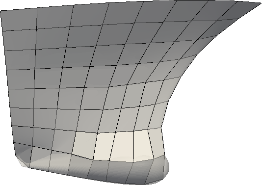
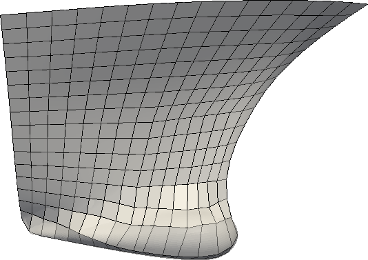
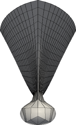
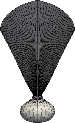
Figure 8: Normal to mesh projection strategy. If the geometry does not intersect the direction normal to the existing points, then the closest point on the shape to the original point – typically lying on the shape boundary – is selected. Panels as in Fig. 7. This strategy produces uniformly distributed cells in all cases.

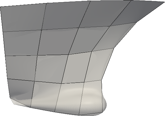
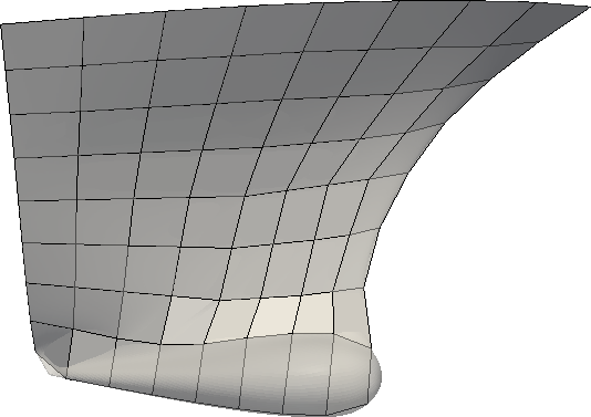
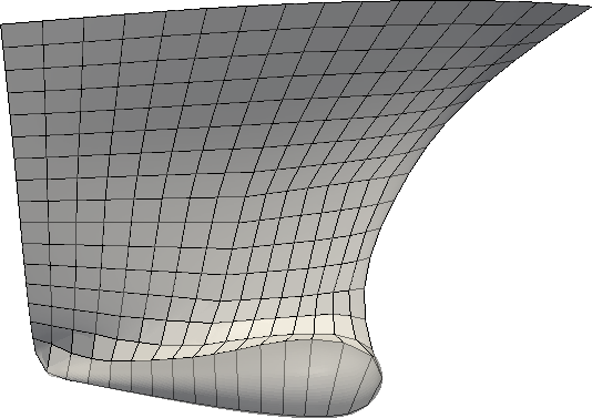
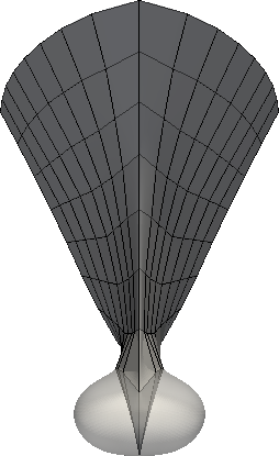
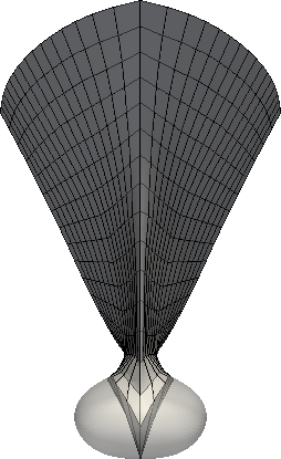
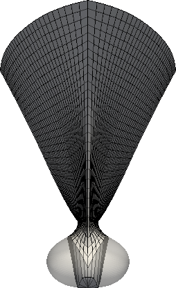
Figure 9: Normal to surface projection strategy. In cases where more than one surface normal projection is available, the closest of them is selected. If the shape is composed by several sub-shapes, the projection is carried out onto every sub-shape and the closest projection point is selected. Panels as in Fig. 7. This strategy is unable to produce well-shaped cells in areas of large curvature.

To illustrate how our approach can be used to generate better meshes, we will use an industrial application that involves meshing a single parametric patch describing the bow portion of one side of the DTMB 5410 ship hull, containing also a sonar dome. The presence of several convex and concave high curvature regions makes such a geometry a particularly meaningful example.

Figures 7–9 show results for this model geometry with the three projection strategies. The directional projection strategy with a horizontal direction of projection (Fig. 7) generally produces high quality meshes except in those places where the geometry is tangent to the projection direction – i.e., in particular at the front of the bulb as well as the bottom. In contrast, using the direction normal to the existing points (Fig. 8) generates high quality meshes everywhere. Finally, the option to use a surface normal instead of a mesh normal vector (Fig. 9) is not only expensive to compute, but here yields meshes that are grossly distorted wherever the geometry has large curvature (i.e., around the bulb); this might also have been expected from the left panel of Fig. 5 that shows a similar effect.

6.2 Refinement strategy based on local maximum curvature

The case of multi-patch geometries is more complicated as small gaps or superimpositions are typically present between neighboring patches. Meshes directly generated from this parameterization will therefore often not be “water-tight”. On the other hand, one can generate a coarse mesh by hand or by software that simply starts with a few points on the surface that are then connected to cells without taking into account the subdivision into patches; such a mesh can then be refined hierarchically to obtain a mesh of sufficient density.

In the following, let us show how we can use the results of the previous section towards building meshes for an entire ship hull; we will also show how additional information can be extracted from CAD tools to drive the refinement strategy on CAD based geometries. To this end, Figure 10 depicts a CAD model of a Kriso KCS ship hull – a common benchmark for CFD applications of naval architecture [29]. In this production-like CAD model the patches are not connected in a water-tight fashion and the surface parametrization is not continuous at patch junctions. These defects prevent most mesh generators from obtaining a closed grid.

. .

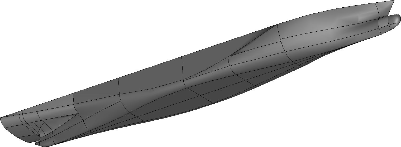
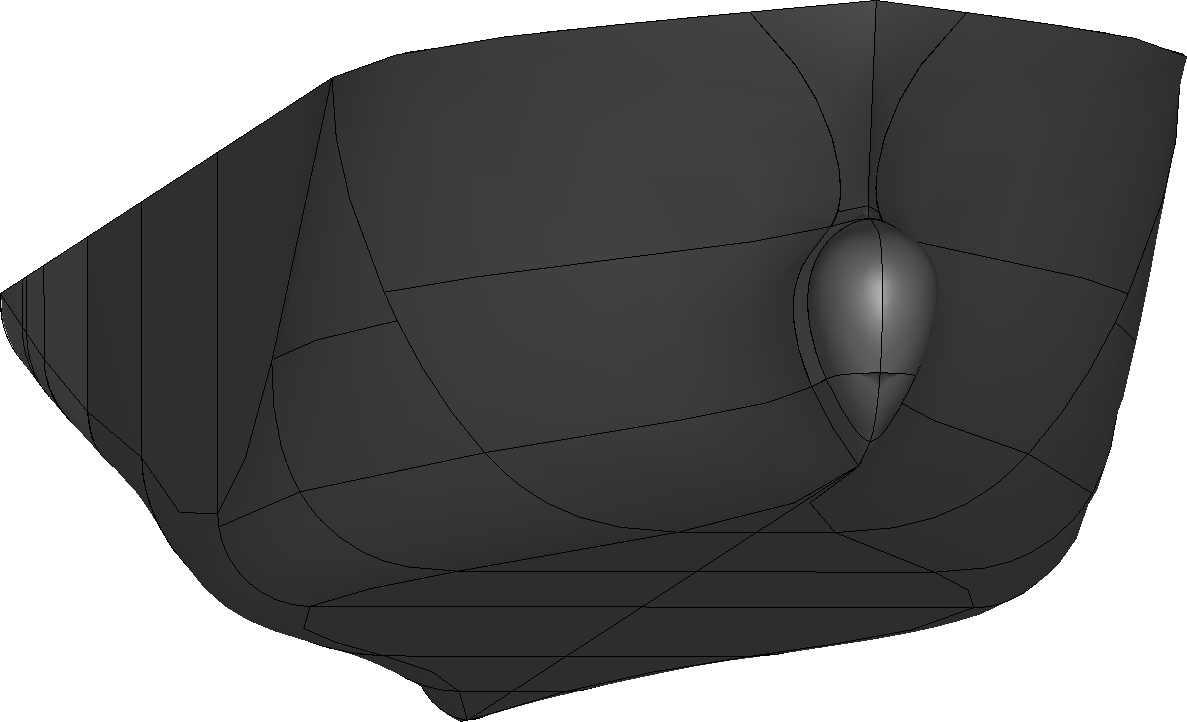
Figure 10: Overall (left) and bow (right) view of the CAD model of a ship hull. The model is composed of approximately 120 parametric patches, delimited by black lines.

We start from a minimal initial surface grid composed of about 40 cells (top panel of Fig. 11) and refine it a number of times using the strategy where we project in a direction normal to the existing points. Refinement of the initial grid starts with an anisotropic refinement step in which cells with an aspect ratio larger then a threshold $\lambda_{\text{max}}$ are cut along their most elongated direction. We then refine the resulting quadrilateral mesh adaptively, using an estimate of the local curvature of the CAD surface as a criterion. This estimate is obtained exploiting a technique essentially identical to the one used in the “Kelly” error estimator [28, 19]. Elements in areas with higher curvature will have larger jumps of the (cell) normal vectors across cell boundaries. The bottom panel of Fig. 11 shows the final grid generated.

Figure 11: Initial (top) and final (bottom) surface grids on the Kriso KCS hull, with 40 and $\tilde{}$ 11,500 quadrilateral cells, respectively.

Despite the fact that the original CAD surface is composed of several unconnected parametric patches, the projection procedure is able to find, for each of the grid nodes, the best projection among those obtained onto individual patches. As a result, the final mesh is water-tight, and independent of the CAD surface parametrization and patch distribution. In addition, the adopted refinement strategy distributes a larger number of new nodes in high curvature regions, ensuring a uniform quality of approximation of the geometry. We show this in more detail in Fig. 12, illustrating the bow and stern portions of the final grid. Finally, it is worth pointing out that for the generation of the grids portrayed in Fig. 11 and Fig. 12, no smoothing stage was carried out in between refinements to enhance mesh quality. Yet, the projection in a direction normal to the existing points allows for retaining the quality of the original coarse grid across more than 10 levels of refinement without any additional adjustment.

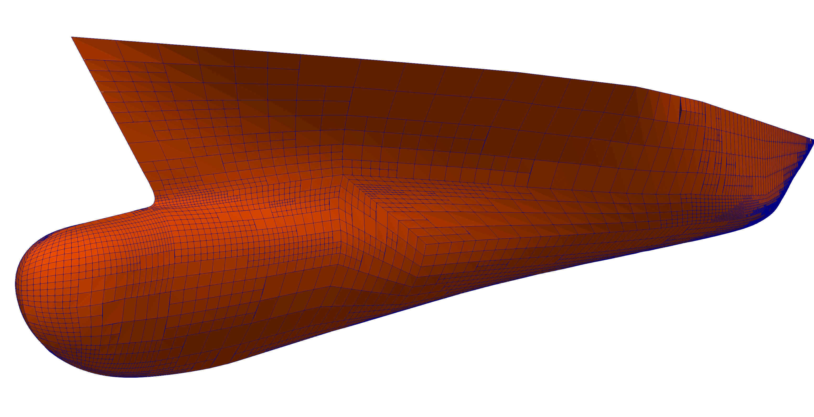
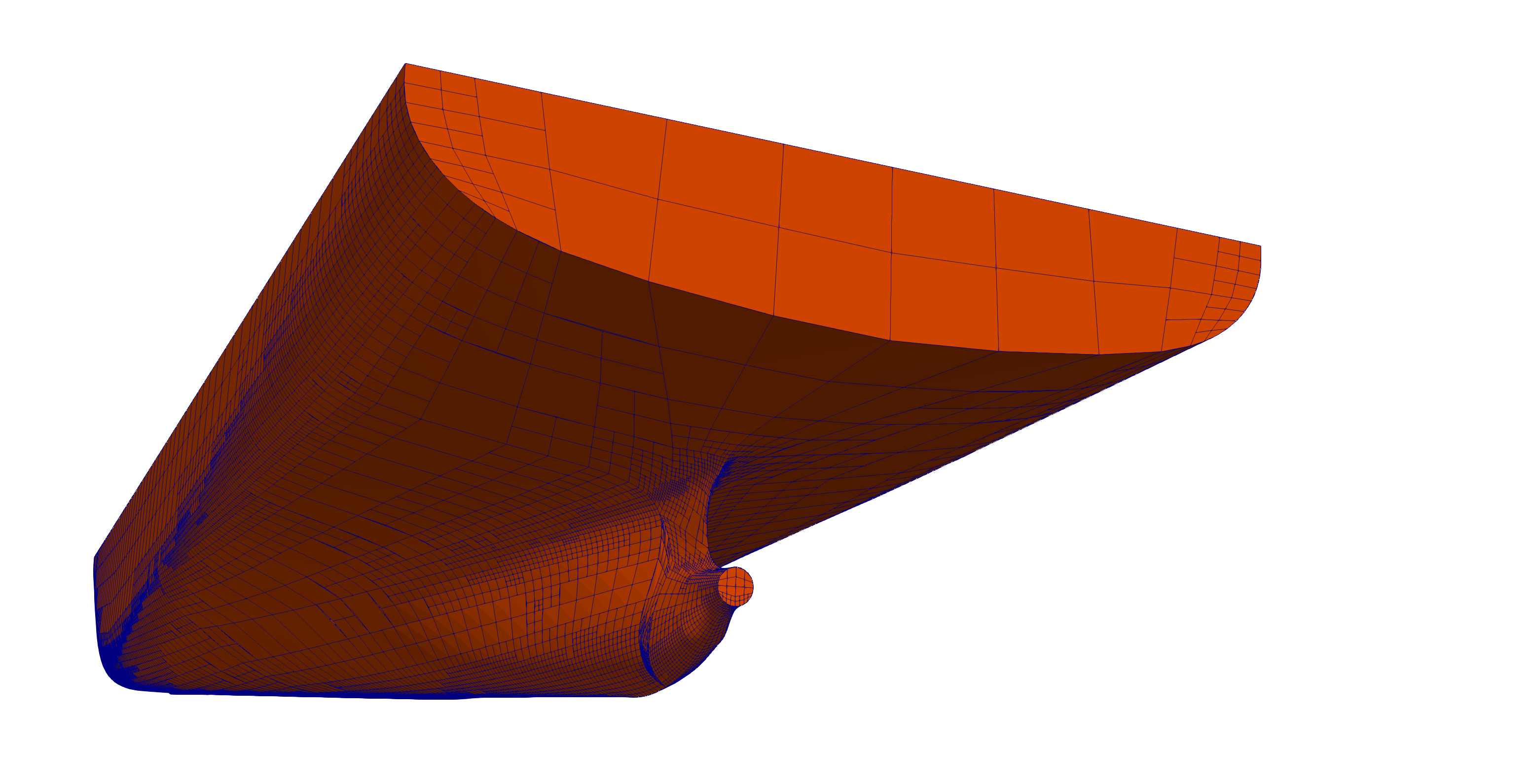
Figure 12: Bow (left) and stern (right) details of the adaptively refined surface grid on the Kriso KCS hull from Figures 10 and 11. The adaptive refinement strategy results in finer cells in high curvature regions, ensuring uniform approximation of the geometry. In addition, the grid is independent of the non-sharp edges separating the 120 parametric patches composing the underlying CAD model. In the final mesh, hanging nodes are placed on the underlying geometry, leading to a non-watertight mesh. However, these artifacts are easily removed by enforcing continuity of the geometry.

6.3 (Ab)Using primitives based on analytic charts for graded meshes

We end this section by outlining how else the primitives can be used to satisfy practical needs. In particular, we can achieve graded mesh refinement strategies based on the explicit definition of a custom metric that describes the manifold with associated push-forward and pull-back operations as discussed in Section 5.1.

Consider, as a simple example, the discretization of the unit square $[0,1]^{2}$. We can provide a non-flat local metric, induced by the following (analytic, invertible) mapping:

$$\begin{split}\phi:[0,1]^{2}&\to[0,1]^{2}\\ (x,y)&\to(x^{2},y^{2}).\end{split}$$

If we consider this mapping for the construction of the new point primitive as described in Section 5.1, we obtain, upon refinement, a graded mesh like in Figure 13, left. But we are not restricted to refining towards left and bottom edges in the figure. Rather, by using more complicated mappings, one can concentrate elements in regions of interest by choosing $\phi$. For example, we can refine towards all four sides of the square (see Figure 13, right) by choosing

$$\phi(x,y)=\left(\frac{1}{2}\sin\left(\pi\left(x-\frac{1}{2}\right)\right)+\frac{1}{2},\frac{1}{2}\sin\left(\pi\left(y-\frac{1}{2}\right)\right)+\frac{1}{2}\right).$$

. .

Figure 13: Example of graded meshes, obtained using simple diffeomorphisms of the unit square.

7 Conclusions

The traditional workflow in finite element, finite volume, or finite difference simulations – split into preprocessing, simulation, and postprocessing stages – is poorly suited to modern numerical methods because information about the underlying geometry is typically not propagated beyond the mesh generation stage. To address this deficiency, we have herein undertaken a comprehensive review of where geometry information is used in simulation software, and what it would take to provide this from typical Constructive Solid Geometry (CSG) or Computer Aided Design (CAD) tools. We have found that, despite the very large number of places in which geometry information is used, all uses can be reduced to just two “primitive” operations: The generation of a new point that interpolates existing points, and the computation of a tangent vector to a line connecting two points. We have then described in detail how these two operations can be implemented for common CSG and CAD cases, and illustrated how these implementations can help create meshes for complex geometries that are both of high quality and respect the underlying geometry.

The methods discussed herein are all available as part of the open source finite element library deal.II [3, 2] and form the basis of propagating geometry information to all parts of the library and application codes built on top of it.

Appendix A An operation that can not be expressed via the two primitives

In our survey of uses of geometric information for Section 3, we have come across just one operation that can not be expressed in terms of the two primitives introduced in Section 2: the computation of second or higher derivatives of finite element shape functions when using the underlying geometry of the domain, rather than a polynomial mapping.

For most “common” finite elements, shape functions are defined on a reference cell and then mapped to each of the cells of the finite element mesh. Let $\hat{K}$ be the reference cell (e.g., the reference triangle or reference square) and $\hat{\varphi}_{i}(\hat{\mathbf{x}}),i=1,\ldots,N$ be the shape functions of a scalar finite element. For a given cell $K$ of the mesh, let $\mathbf{F}_{K}:\hat{K}\mapsto K$ be the mapping, assuming that $K$ is part of the underlying geometry, rather than a polynomial approximation of it. In that case, $\mathbf{F}_{K}$ is, in general, not polynomial. The shape functions we will then work with are $\varphi_{i}(\mathbf{x})=\hat{\varphi}_{i}(\mathbf{F}_{K}^{-1}(\mathbf{x}))$.

By the chain rule, the derivatives, in real space, of shape functions at an evaluation point $\hat{\mathbf{x}}_{q}$ are then given by

$$\nabla\varphi_{i}(\mathbf{x}_{q}) =J_{K}^{-1}\hat{\nabla}\hat{\varphi}_{i}(\hat{\mathbf{x}}_{q}),$$

where $J_{K}=\frac{\partial\mathbf{x}}{\partial\hat{\mathbf{x}}}=\frac{\partial\mathbf{F}_{K}(\hat{\mathbf{x}})}{\partial\hat{\mathbf{x}}}$ is the Jacobian of the transformation. This matrix, and its inverse, are easily computed for both polynomial mappings (see Section 3.2) and for exact mappings (see Section 3.3). However, for some applications, it is also necessary to compute second or even higher derivatives of shape functions. An example is the evaluation of the residual of a finite element solution for second or higher order operators. Others include the evaluation of the bilinear form for the biharmonic equation, and the evaluation of the Hessian of (a component of) the solution for purposes of defining anisotropic mesh refinement indicators. In these cases, we can compute (with appropriate contraction over the various indices of the objects in the formula)

$$\nabla^{2}\varphi_{i}(\mathbf{x}_{q}) =J_{K}^{-1}\hat{\nabla}\left[J_{K}^{-1}\hat{\nabla}\hat{\varphi}_{i}(\hat{\mathbf{x}}_{q})\right]$$

$$=J_{K}^{-1}J_{K}^{-1}\hat{\nabla}^{2}\hat{\varphi}_{i}(\hat{\mathbf{x}}_{q})+J_{K}^{-1}\left[\hat{\nabla}[J_{K}^{-1}]\right]\hat{\varphi}_{i}(\hat{\mathbf{x}}_{q})$$

$$=J_{K}^{-1}J_{K}^{-1}\hat{\nabla}^{2}\hat{\varphi}_{i}(\hat{\mathbf{x}}_{q})-J_{K}^{-1}\left[J_{K}^{-1}(\hat{\nabla}J_{K})J_{K}^{-1}\right]\hat{\varphi}_{i}(\hat{\mathbf{x}}_{q}),$$

where we have made use of the equality $0=\hat{\nabla}(J_{K}J_{K}^{-1})=(\hat{\nabla}J_{K})J_{K}^{-1}+J_{K}(\hat{\nabla}[J_{K}^{-1}])$.

This representation of second derivatives (and formulas for even higher derivatives) requires computing derivatives of $J_{K}$. This is not a complication for the usual, polynomial mappings such as those discussed in Section 3.2, since all we need to do is determine the appropriate interpolation points, construct the polynomial approximation, and then take derivatives of this polynomial. On the other hand, for “exact” mappings, no explicit representation of the mapping is available. We can only use the new point primitive to evaluate $\mathbf{F}_{K}$, and use the tangent vector primitive to compute the derivative $J_{K}=\hat{\nabla}\mathbf{F}_{K}$, but we have no way of evaluating the derivative of $J_{K}$ (i.e., the second derivatives of $\mathbf{F}_{K}$).

Remark 4

One could of course define a third primitive to also aid the computation of this information. (See also Remark 3.) On the other hand, our goal in this paper is to point out a minimal interface that geometry packages have to satisfy to support the most common finite element operations. Since all finite element packages we are aware of support polynomial geometry approximations, we consider the two operations defined in Section 2 as sufficient and defer the definition of additional primitives necessary for the operation discussed in this section to separate work.

Alternatively, one can approximate $\hat{\nabla}J_{K}$ by finite differencing the matrix $J_{K}$, which we already know how to compute.

Appendix B Periodic domains

In practice, one frequently encounters domains that are periodic in at least one direction, or for which at least the push-forward function is periodic. An example is a domain that consists of the surface of a cylinder. Another would be a situation where one only considers a segment of a cylinder surface – in that case, the domain itself is not periodic, but both the image and pre-image of the push-forward function are. Such cases present interesting questions for the implementation of the new point primitive. If we can answer these appropriately, we will know how to deal with the tangent vector primitive by using relationship (1).

In our implementation in deal.II, primitives based on pull-back and push-foward functions are provided by the ChartManifold class that allows one to specify along which direction in the reference Euclidean patch $U_{\alpha}^{\ast}$ periodicity should be considered, and what the periodicity period $L$ along that direction is. Specifically, periodicity affects the way the new point oracle computes the middle point between two neighboring points: If two points are more than half a period distant in the Euclidean reference patch $U_{\alpha}^{\ast}$, then their distance should be computed by crossing the periodicity boundary, i.e., the weighted average of the two points should be computed by adding a half period to the sum of the two. For example, if along a direction we have a periodic manifold, with period of $2\pi$, then the average of $(2\pi-\epsilon)$ and $(\epsilon)$ along the periodic domain (computed with equal weights) should not return $\pi$, but $2\pi$ (or, equivalently, zero). On the manifold, these two points are truly at a distance $2\epsilon$ and not $(2\pi-\epsilon)$ (see Figure 14 for an example of this process).

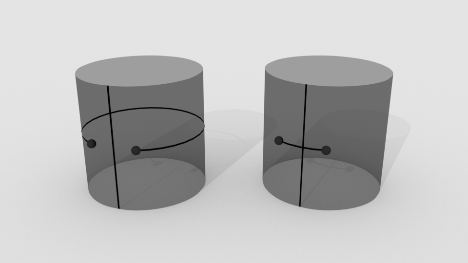
Figure 14: Effect of periodicity when computing the new point primitive with two points close to the gluing edge of a cylinder. If periodicity is not taken into account, the path used to compute the averages does not cross the gluing edge (left), and new points would end up on the line that turns around the cylinder. When taking periodicity into account, the shortest path is used when computing averages (right), and new points end up on the line that crosses the gluing edge.

The periodicity treatment becomes ill posed for cases in which the distance of two points is exactly a half period. Then, either direction would be possible, and no unique solution exists. The straight forward way to solve this issue is to ensure that there are no points at exactly this distance, by providing a slightly more refined initial grid.

References

- [1] M. Ainsworth and J. T. Oden. A Posteriori Error Estimation in Finite Element Analysis. John Wiley and Sons, 2000.
- [2] D. Arndt, W. Bangerth, T. C. Clevenger, D. Davydov, M. Fehling, D. Garcia-Sanchez, G. Harper, T. Heister, L. Heltai, M. Kronbichler, R. M. Kynch, M. Maier, J.-P. Pelteret, B. Turcksin, and D. Wells. The deal.II library, version 9.1. J. Numer. Math., 27(4):203–213, Dec. 2019.
- [3] D. Arndt, W. Bangerth, D. Davydov, T. Heister, L. Heltai, M. Kronbichler, M. Maier, J.-P. Pelteret, B. Turcksin, and D. Wells. The deal.II finite element library: design, features, and insights. Computers & Mathematics with Applications, 81:407–422, 2021.
- [4] I. Babuška and T. Strouboulis. The Finite Element Method and its Reliability. Clarendon Press, New York, 2001.
- [5] W. Bangerth and R. Rannacher. Adaptive Finite Element Methods for Differential Equations. Birkhäuser Verlag, 2003.
- [6] S. Bartels, C. Carstensen, and G. Dolzmann. Inhomogeneous dirichlet conditions in a priori and a posteriori finite element error analysis. Numerische Mathematik, 99(1):1–24, Sept. 2004.
- [7] F. Bassi and S. Rebay. High-order accurate discontinuous finite element solution of the 2D Euler equations. J. Comput. Phys., 138(2):251–285, 1997.
- [8] P. K. Bhattacharyya and N. Nataraj. On the combined effect of boundary approximation and numerical integration on mixed finite element solution of 4th order elliptic problems with variable coefficients. ESAIM: Mathematical Modelling and Numerical Analysis, 33(4):807–836, 1999.
- [9] D. Braess. Finite Elements. Cambridge University Press, 2007.
- [10] W. L. Briggs, V. E. Henson, and S. F. McCormick. A Multigrid Tutorial. SIAM, second edition, 2000.
- [11] S. R. Buss and J. P. Fillmore. Spherical averages and applications to spherical splines and interpolation. ACM Trans. Graphic., 20(2):95–126, 2001.
- [12] G. F. Carey. Computational Grids: Generation, Adaptation and Solution Strategies. Taylor & Francis, 1997.
- [13] P. G. Ciarlet and P.-A. Raviart. The combined effect of curved boundaries and numerical integration in isoparametric finite element methods. In The Mathematical Foundations of the Finite Element Method with Applications to Partial Differential Equations, pages 409–474. Elsevier, 1972.
- [14] P. G. Ciarlet and P.-A. Raviart. Interpolation theory over curved elements, with applications to finite element methods. Comput. Meth. Appl. Mech. Engrg., 1(2):217–249, Aug. 1972.
- [15] T. C. Clevenger, T. Heister, G. Kanschat, and M. Kronbichler. A flexible, parallel, adaptive geometric multigrid method for FEM. ACM Trans. Math. Softw., 47(1):7:1–27, 2021.
- [16] V. Dobrev, P. Knupp, T. Kolev, K. Mittal, and V. Tomov. The target-matrix optimization paradigm for high-order meshes. SIAM Journal on Scientific Computing, 41(1):B50–B68, 2019.
- [17] W. Dörfler and M. Rumpf. An adaptive strategy for elliptic problems including a posteriori controlled boundary approximation. Math. Comp., 67:1361–1382, 1998.
- [18] G. Farin. Curves and surfaces for CAGD: A practical guide. Morgan Kaufmann, San Francisco, CA, USA, 5th edition, 2002.
- [19] J. P. d. S. R. Gago, D. W. Kelly, O. C. Zienkiewicz, and I. Babuška. A posteriori error analysis and adaptive processes in the finite element method: Part II — Adaptive mesh refinement. Int. J. Num. Meth. Engrg., 19:1621–1656, 1983.
- [20] N. Giuliani, A. Mola, L. Heltai, and L. Formaggia. FEM SUPG stabilisation of mixed isoparametric BEMs: application to linearised free surface flows. Engineering Analysis with Boundary Elements, 59:8–22, 2015.
- [21] W. J. Gordon and L. C. Thiel. Transfinite mappings and their application to grid generation. Appl. Math. Comput., 10:171–233, 1982.
- [22] R. Hartmann. Adaptive Finite Element Methods for the Compressible Euler Equations. PhD thesis, University of Heidelberg, 2002.
- [23] T. Heister, J. Dannberg, R. Gassmöller, and W. Bangerth. High accuracy mantle convection simulation through modern numerical methods. II: Realistic models and problems. Geophysical Journal International, 210:833–851, 2017.
- [24] T. Heister, Y. Zhou, W. Bangerth, and D. Wells. The deal.II tutorial: step-49. https://www.dealii.org/developer/doxygen/deal.II/step_49.html, 2013.
- [25] J. S. Hesthaven and T. Warburton. Nodal discontinuous Galerkin methods: algorithms, analysis, and applications. Springer, 2007.
- [26] F. Hindenlang, T. Bolemann, and C. D. Munz. Mesh curving techniques for high order discontinuous Galerkin simulations. In Notes on Numerical Fluid Mechanics and Multidisciplinary Design, pages 133–152. Springer International Publishing, 2015.
- [27] U. P. D. A. IGES/PDES Organization. Initial Graphics Exchange Specification: IGES 5.3. US Product Data Association, 1996.
- [28] D. W. Kelly, J. P. d. S. R. Gago, O. C. Zienkiewicz, and I. Babuška. A posteriori error analysis and adaptive processes in the finite element method: Part I–error analysis. Int. J. Num. Meth. Engrg., 19:1593–1619, 1983.
- [29] W. Kim, S. Van, and D. Kim. Measurement of flows around modern commercial ship models. Experiments in Fluids, 31:567–578, 2001.
- [30] N. Krais, A. Beck, T. Bolemann, H. Frank, D. Flad, G. Gassner, F. Hindenlang, M. Hoffmann, T. Kuhn, M. Sonntag, and C.-D. Munz. FLEXI: A high order discontinuous galerkin framework for hyperbolic–parabolic conservation laws. Comput. Math. Appl., 81:186–219, 2021.
- [31] M. Kronbichler, T. Heister, and W. Bangerth. High accuracy mantle convection simulation through modern numerical methods. Geophys. J. Int., 191:12–29, 2012.
- [32] L. Mansfield. Approximation of the boundary in the finite element solution of fourth order problems. SIAM Journal on Numerical Analysis, 15(3):568–579, June 1978.
- [33] S. Marjudi, M. F. M. Amran, K. A. Abdullah, S. Widyarto, N. A. A. M. Majid, and R. Sulaiman. A review and comparison of IGES and STEP. In Proceedings Of World Academy Of Science, Engineering And Technology, pages 1013–1017, 2010.
- [34] G. Mengaldo, D. Moxey, M. Turner, R. C. Moura, A. Jassim, M. Taylor, J. Peiro, and S. J. Sherwin. Industry-relevant implicit large-eddy simulation of a high-performance road car via spectral/hp element methods, 2020.
- [35] K. Mittal and P. F. Fischer. Mesh smoothing for the spectral element method. Journal of Scientific Computing, 78(2):1152–1173, 2019.
- [36] A. Mola, L. Heltai, and A. Desimone. A stable and adaptive semi-Lagrangian potential model for unsteady and nonlinear ship-wave interactions. Engineering Analysis with Boundary Elements, 37(1), 2013.
- [37] A. Mola, L. Heltai, and A. DeSimone. Wet and dry transom stern treatment for unsteady and nonlinear potential flow model for naval hydrodynamics simulations. Journal of Ship Research, 61(1):1–14, mar 2017.
- [38] D. Moxey, C. D. Cantwell, Y. Bao, A. Cassinelli, G. Castiglioni, S. Chun, E. Juda, E. Kazemi, K. Lackhove, J. Marcon, G. Mengaldo, D. Serson, M. Turner, H. Xu, J. Peiró, R. M. Kirby, and S. J. Sherwin. Nektar++: Enhancing the capability and application of high-fidelity spectral/hp element methods. Comput. Phys. Commun., 249:107110, 2020.
- [39] D. Moxey, D. Ekelschot, U. Keskin, S. J. Sherwin, and J. Peiró. High-order curvilinear meshing using a thermo-elastic analogy. Computer-Aided Design, 72:130–139, 2016.
- [40] M. J. Pratt. ISO 10303, the STEP standard for product data exchange, and its PLM capabilities, 2005.
- [41] O. C. S.A.S. Opencascade technology, 2010. http://www.opencascade.org.
- [42] S. A. Sauter and C. Schwab. Boundary element methods, volume 39 of Springer Series in Computational Mathematics. Springer Berlin Heidelberg, Berlin, Heidelberg, 2011.
- [43] G. Strang and G. F. Fix. An analysis of the finite element method. Wellesley-Cambridge Press, Wellesley, MA, USA, 1988.
- [44] P. Šolín, K. Segeth, and I. Doležel. High-order finite element methods. Chaptman & Hall/CRC, Boca Raton, FL, USA, 2004.