A data-driven model of nucleosynthesis with chemical tagging in a lower-dimensional latent space

Abstract

Chemical tagging seeks to identify unique star formation sites from present-day stellar abundances. Previous techniques have treated each abundance dimension as being statistically independent, despite theoretical expectations that many elements can be produced by more than one nucleosynthetic process. In this work we introduce a data-driven model of nucleosynthesis where a set of latent factors (e.g., nucleosynthetic yields) contribute to all stars with different scores, and clustering (e.g., chemical tagging) is modelled by a mixture of multivariate Gaussians in a lower-dimensional latent space. We use an exact method to simultaneously estimate the factor scores for each star, the partial assignment of each star to each cluster, and the latent factors common to all stars, even in the presence of missing data entries. We use an information-theoretic Bayesian principle to estimate the number of latent factors and clusters. Using the second Galah data release we find that six latent factors are preferred to explain $N=$ 2,566 stars with 17 chemical abundances. We identify the rapid- and slow-neutron capture processes, as well as latent factors consistent with Fe-peak and $\alpha$-element production, and another where K and Zn dominate. When we consider $N\sim$ 160,000 stars with missing abundances we find another seven factors, as well as 16 components in latent space. Despite these components showing separation in chemistry that is explained through different yield contributions, none show significant structure in their positions or motions. We argue that more data, and joint priors on cluster membership that are constrained by dynamical models, are necessary to realise chemical tagging at a galactic-scale. We release accompanying software that scales well with the available data, allowing for model parameters to be optimised in seconds given a fixed number of latent factors, components, and $\sim 10^{7}$ abundance measurements.

1 Introduction

The detailed chemical abundances that are observable in a star’s photosphere provide a fossil record that carries with it information about where and when that star formed (Freeman & Bland-Hawthorn, 2002). While the photospheric abundances remain largely unchanged throughout a star’s lifetime (however see Dotter et al., 2017; Ness et al., 2018a), the dynamical dissipation timescale of open clusters in the Milky Way disc is of order a few gigayears (Portegies Zwart et al., 1998). That makes chemical tagging an attractive approach to identify star formation sites long after those stars are no longer gravitationally bound to each other.

Gravitationally bound star clusters have been useful laboratories for testing the limits and utility of chemical tagging. Although biases arise when only considering star clusters that are still gravitationally bound, the chemical homogeneity of open clusters provides an empirical measure of how similar stars would need to be before they could be tagged as belonging to the same star formation site (Bland-Hawthorn et al., 2010a, b; Mitschang et al., 2014). However, there are analysis issues in understanding how precisely those chemical abundances can be measured (Bovy, 2016), and how chemically similar stars can be that did not form together (dopplegängers; Ness et al., 2018b). If open clusters were truely chemically homogeneous then under idealistic assumptions our ability to chemically tag the Milky Way would depend primarily on the precision with which we can measure those chemical abundances in stars. Data-driven approaches to modelling stellar spectra are improving upon this precision (Ness et al., 2015; Ness, 2018; Ness et al., 2018a; Casey et al., 2016a, 2017; Ho et al., 2017a, b; Leung & Bovy, 2018; Ting et al., 2019), but more work is needed: astronomers have not yet developed unbiased estimators of chemical abundances that saturate the Cramér-Rao bound (Cramér, 1946; Rao, 1945).

Chemical tagging experiments require a catalogue of precise chemical abundance measurements for a large number of stars, where those chemical abundances trace different nucleosynthetic pathways. This is the primary goal of the Galactic Archaeology with HERMES (Galah) survey (De Silva et al., 2015; Martell et al., 2017; Buder et al., 2018), a stellar spectroscopic survey that uses the High Efficiency and Resolution Multi-Element Spectrograph (HERMES; Sheinis et al., 2015) on the 3.9 m Anglo-Australian Telescope (AAT). Galah will observe up to $10^{6}$ stars in the Milky Way, and measure up to 30 chemical abundances for each star (Bland-Hawthorn & Sharma, 2016). This includes light odd-Z elements (e.g., Na, K), elements produced through alpha-particle capture (e.g., Mg, Ca), and elements produced through the slow (e.g., Ba) and rapid neutron-capture process (e.g., Eu). No other current or planned spectroscopic survey provides an equivalent set of chemical abundances for a comparable number of stars.

Given these data and the most favourable assumptions in chemical tagging – that star clusters are truely chemically homogenous, that we can measure those abundances with infinite precision, and that those abundances are differentiable between star clusters – then chemical tagging becomes a clustering problem. All clustering techniques applied to chemical tagging thus far have assumed that the data dimensions are independent. That is to say that adding a dimension of say [Ni/H] provides independent information that could not have been predicted from other elemental abundances. Theory and observations agree that this cannot be true. Nucleosynthetic processes produce multiple elements in varying quantities, and the effective dimensionality of stellar abundance datasets has been shown to be lower than the actual number of abundance dimensions (Ting et al., 2012; Price-Jones & Bovy, 2018; Milosavljevic et al., 2018). Any clustering approach that treats each new elemental abundance as an independent axis of information will therefore conclude with biased inferences about the star formation history of our Galaxy.

It is not trivial to confidently estimate the nucleosynthetic yields that have contributed to the chemical abundances of each star. There are qualitative statements that can be made for large numbers of stars, or particular types of stars, but quantifying the precise contribution of different processes to each star is an unsolved problem. For example, the so-called [$\alpha$/Fe] ‘knee’ in abundance ratios in the Milky Way can qualitatively be explained by core-collapse supernovae being the predominant nucleosynthetic process in the early Milky Way before Type Ia supernovae made a significant contribution, but efforts to date have not sought to try to explain the detailed abundances of stars as a contribution of yields from different systems (however see West & Heger, 2013). This is in part because of the challenging and degenerate nature of the problem as described, and is complicated by the differences in yield predictions that account from prescriptions used in different theoretical models.

New approaches to chemical tagging are clearly needed. Immediate advances would include methods that take the dependence among chemical elements into account within some generative model, or techniques that combine chemical abundances with dynamical constraints to place joint prior probabilities on whether any two stars could have formed from the same star cluster, given some model of the Milky Way.

In this work we focus on the former. Here we present a new approach to chemical tagging that allows us to identify the latent (unobserved) factors that contribute to the chemical abundances of all stars (e.g., nucleosynthetic yields) while simultaneously performing clustering in the latent space. Notwithstanding caveats that we will discuss in detail, this allows us to infer nucleosynthetic yields rather than strictly prescribe them from models. Moreover, the scale of the clustering problem reduces by a significant fraction because the clustering is performed in a lower dimensional latent space instead of the higher dimensional data space. In Section 2 we describe the model and the methods we use to estimate the model parameters. Section 3 describe the experiments performed using generated and real data sets. We discuss the results of these experiments in Section 4, including the caveats with the model as described. We conclude in Section 5.

2 Methods

Latent factor analysis is a common statistical approach for describing correlated observations with a lower number of latent variables (e.g., Thompson, 2004). Related techniques include principal component analysis (Hotelling, 1933) and its variants (Tipping & Bishop, 1999), singular value decomposition (Golub & Reinsch, 1970), and other matrix factorization methods. While factor analysis on its own is a useful dimensionality reduction tool to identify latent factors that contribute to the chemical abundances of stars (e.g., Ting et al., 2012; Price-Jones & Bovy, 2018; Milosavljevic et al., 2018), factor analysis cannot describe clustering in the data (or latent) space. As a result, some works have performed clustering and then required different latent factors for each (totally assigned) component (e.g., Edwards & Dowe, 1998). Similarly, clustering techniques applied to chemical abundances to date (e.g., Hogg et al., 2016) do not account for the lower effective dimensionality in elemental abundances.

Here we expand on a variant of factor analysis known elsewhere as a mixture of common factor analyzers (Baek et al., 2010), where the data are generated by a set of latent factors that are common to all data, but the scoring (or extent) of those factors is different for each data point, and the data can be modelled as a mixture of multivariate normal distributions in the latent space (factor scores). In this work the data $\boldsymbol{\mathbf{X}}$ is a $D\times N$ matrix where $N$ is the number of stars and $D$ is the number of chemical abundances measured for each star. We assume a generative model for the data

$$\boldsymbol{\mathbf{X}}=\boldsymbol{\mathbf{\mu}}+\textbf{L}\textbf{S}+\boldsymbol{\mathbf{e}}$$ (1)

where L is a $D\times J$ matrix of factor loads that is common to all data points, $J$ is the number of latent factors, and the factor scores for the $n^{\mathrm{th}}$ data point

$$\textbf{S}_{n}\sim\mathcal{N}(\boldsymbol{\mathbf{\xi}}_{k},\boldsymbol{\mathbf{\Omega}}_{k})$$ (2)

are drawn from the $k^{\mathrm{th}}$ multivariate normal distribution, where each $k^{\mathrm{th}}$ component has a $J$-dimensional mean and a dense $J\times J$ covariance matrix. The mean vector $\boldsymbol{\mathbf{\mu}}$ describes the mean datum in each dimension. The factor scores for all data points S is then a $J\times N$ matrix, where each data point has a partial association to the components in latent space. We assume $\boldsymbol{\mathbf{e}}\sim\mathcal{N}\left(\boldsymbol{\mathbf{0}},\textrm{diag}(\boldsymbol{\mathbf{D}})\right)$ is independent of the latent space, and $\boldsymbol{\mathbf{D}}$ is a vector of variances in each $D$ abundance dimensions. In this model each data point can be represented as being drawn from a mixture of multivariate normal components, except the components are clustered in the latent space S and projected into the data space by the factor loads L. In a sense we are using latent factor analysis as a form of dimensionality reduction and simultaneously performing clustering in latent space .

We assume that the latent space is lower dimensionality than the data space (i.e., $J<D$). Within the context of stellar abundances, the factor loads L can be thought of as the mean yields of nucleosynthetic events (e.g., $s$-process production from AGB stars averaged over initial mass function and star formation history), and the factor scores are analogous to the relative counts of those nucleosynthetic events. The clustering in factor scores achieves the same as a clustering procedure in data space, except we simultaneously estimate the latent processes that are common to all stars (the so-called factor loads, analogous to nucleosynthetic yields). Within this framework a rare nucleosynthetic event can still be described as a ‘factor load’ $\textbf{L}_{j}$, but its rarity would be represented by associated factor scores being zero for most stars and thus have no contribution to the observed abundances. In practice the factor loads can only be identified up to orthogonality and cannot be expressly interpreted as nucleosynthetic yields because they have limited physical meaning (we discuss this further in Section 4), but this description of typical yields and relative event rates should help build intuition for the model parameters, and provide context within the astrophysical problem it is being applied.

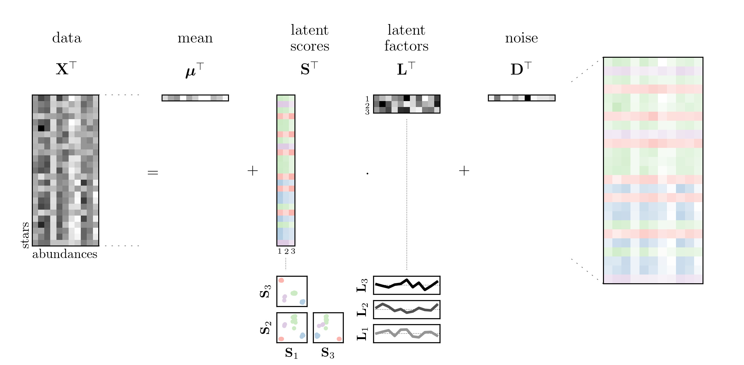
Figure 1:

Including latent factors in the model description allows us to account for processes that affect multiple elemental abundances. In this way we are accounting for the fact that the data dimensions are not independent of each other. Another benefit is the scaling with computational cost. If we considered data sets of order $10^{7.5}$ entries (e.g., 30 chemical abundances for $10^{6}$ stars) purely as a clustering problem, then even the most efficient clustering algorithms would incur a significant cumulative computational overhead by searching the parameter space for the number of clusters, and the optimal model parameters given that number of components. However, because the mixture of factor analyzers approach assumes that there is a lower dimensional latent space in which the data are clustered, and that clustering is projected into real space by common factor loads, the dimensionality of the clustering problem is reduced from $N\times D$ to $N\times J$. This reduces computational cost through faster execution of each optimization step, and on average fewer optimization steps needed to reach a specified convergence threshold.

From a statistical standpoint, the primary advantage to using a mixture of factor analysers is that we can simultaneously estimate latent factors (e.g., infer nucleosynthetic yields) and perform clustering (e.g., chemical tagging) within a statistically consistent framework. That is to say that we have a generative data-driven model that can quantitatively describe nucleosynthetic yields, and the factor scores can explain the variance in turbulence and gas mixing, or star formation efficiency, and the parameters of this model can be simultaneously estimated in a self-consistent way with a single scalar-justified objective function.

Without loss of generality the density of the mean-subtracted data $\boldsymbol{\mathbf{X}}-\boldsymbol{\mathbf{\mu}}$ (which we hereafter will refer to simply as Y) can be described as

$$f(\boldsymbol{\mathbf{\textbf{Y}}};\boldsymbol{\mathbf{\Psi}})=\sum_{k=1}^{K}\pi_{k}\phi(\boldsymbol{\mathbf{\textbf{Y}}};\textbf{L}\boldsymbol{\mathbf{\xi}}_{k},\textbf{L}\boldsymbol{\mathbf{\Omega}}_{k}\textbf{L}^{\intercal}+\textrm{diag}(\boldsymbol{\mathbf{D}}))$$ (3)

given $J$ common factor loadings and $K$ components clustered in the latent (factor score) space. Here the parameter vector $\boldsymbol{\mathbf{\Psi}}$ includes $\{\textbf{L},\boldsymbol{\mathbf{\pi}},\boldsymbol{\mathbf{\xi}},\boldsymbol{\mathbf{\Omega}},\boldsymbol{\mathbf{D}}\}$, and $\phi(\boldsymbol{\mathbf{\textbf{Y}}};\boldsymbol{\mathbf{\theta}})$ describes the density of a multivariate Gaussian distribution, and $\pi_{k}$ describes the relative weighting of the $k^{\mathrm{th}}$ component in latent space and $\sum\boldsymbol{\mathbf{\pi}}_{k}=1$. The log likelihood is then given by

$$\log\mathcal{L}(\boldsymbol{\mathbf{\textbf{Y}}}|\boldsymbol{\mathbf{\Psi}})=\sum_{n=1}^{N}\log{f(\boldsymbol{\mathbf{\textbf{Y}}};\boldsymbol{\mathbf{\Psi}})}\quad.$$ (4)

The model as described is indeterminate in that there is no unique solution for the factor loads L and scores S. These quantities can only be determined up until orthogonality in L. However, as we will describe in Section 2.2, with suitable priors on $\boldsymbol{\mathbf{\Psi}}$ one can efficiently estimate the model parameters using the expectation-maximization algorithm (Dempster et al., 1977).

2.1 Initialisation

Here we describe how the model parameters are initialised. To initialise the factor loads L we start by randomly drawing a $D\times D$ matrix from a Haar distribution (Haar, 1933), which is uniform on the special orthogonal group $\textrm{SO}(n)$ and therefore guaranteed to return an orthogonal matrix with a determinant of unity (Stewart, 1980). We denote the $J\times D$ left-most region of this matrix to be our initial guess of L, which provides a set of mutually orthogonal vectors.

We then initially assign each data point as belonging to one of the $K$ components using the k-means++ algorithm (Arthur & Vassilvitskii, 2007) in the latent space. Given the initial factor loads and assignments, we then estimate the relative weights $\boldsymbol{\mathbf{\pi}}$, the mean factor scores of each component $\boldsymbol{\mathbf{\xi}}$, and the covariance matrix of factor scores of each component $\boldsymbol{\mathbf{\Omega}}$. Finally, we initialise the specific variance $\boldsymbol{\mathbf{D}}$ in each dimension as the variance in each data dimension. Other initialisation methods for the latent factors include singular value decomposition (Golub & Reinsch, 1970) or generating random noise with orthogonal constraints, and random assignment is an alternative method that is available for initialising assignments.

Throughout this work we repeat this initialisation procedure 25 times for every trial of $J$ and $K$ for a given data set. We then run expectation-maximization (Section 2.2) from each initialisation until the log likelihood improves by less than $10^{-5}$ per step, and we adopt the model with the highest log likelihood as the preferred model given that trial of $J$, $K$, and the data. Although this optimisation procedure is not convex, in practice it is normally sufficient to initialise from many points to avoid local minima.

2.2 Expectation-Maximization

We use the expectation-maximization algorithm to estimate the model parameters (Dempster et al., 1977). With each expectation step we evaluate the log likelihood given the model parameters $\boldsymbol{\mathbf{\Psi}}$, the message length, and the $N\times K$ responsibility matrix $\boldsymbol{\mathbf{\tau}}$ whose entries are the posterior probability that the $n$th data point is associated to the $k$th component, given the data Y and the current estimate of the parameter vector $\boldsymbol{\mathbf{\Psi}}$:

$$\tau_{nk}=\frac{\pi_{k}\phi(\boldsymbol{\mathbf{\textbf{Y}}}_{n};\textbf{L}\boldsymbol{\mathbf{\xi}}_{k},\textbf{L}\boldsymbol{\mathbf{\Omega}}_{k}\textbf{L}^{\intercal}+\textrm{diag}(\boldsymbol{\mathbf{D}}))}{\sum_{g=1}^{G}\pi_{g}\phi(\boldsymbol{\mathbf{\textbf{Y}}}_{n};\textbf{L}\boldsymbol{\mathbf{\xi}}_{g},\textbf{L}\boldsymbol{\mathbf{\Omega}}_{g}\textbf{L}^{\intercal}+\textrm{diag}(\boldsymbol{\mathbf{D}}))}\quad.$$ (5)

At the maximization step we update our estimates of the parameters $\boldsymbol{\mathbf{\Psi}}$, conditioned on the data Y and the responsibility matrix $\boldsymbol{\mathbf{\tau}}$. The updated parameters estimates are found by setting the second derivative of the log likelihood (Eq. 4) to zero and solving for the parameter values. In doing so this guarantees that every updated estimate of the model parameters is guaranteed to increase the log likelihood. Although there are no guarantees against converging on local minima, in practice it is sufficient to run expectation-maximization from multiple initialisations (as we do) in order to ensure that the global minimum is reached. At the maximization step we first update our estimate of the relative weights $\boldsymbol{\mathbf{\pi}}^{\textrm{(t+1)}}$ given the responsibility matrix $\boldsymbol{\mathbf{\tau}}$

$$\pi_{k}^{\textrm{(t+1)}}=\frac{1}{N}\sum_{n=1}^{N}\tau_{nk}$$ (6)

where the $\boldsymbol{\mathbf{\Psi}}^{\textrm{(t)}}$ superscript refers to the current parameter estimates and $\boldsymbol{\mathbf{\Psi}}^{\textrm{(t+1)}}$ refers to the updated estimate for the next iteration. The updated estimates of the mean factor scores $\boldsymbol{\mathbf{\xi}}^{\textrm{(t+1)}}$ for each component are then given by

$$\boldsymbol{\mathbf{\xi}}_{k}^{\textrm{(t+1)}}=\boldsymbol{\mathbf{\xi}}_{k}^{\textrm{(t)}}+\frac{\boldsymbol{\mathbf{G}}^{\intercal}(\boldsymbol{\mathbf{\textbf{Y}}}^{\intercal}-\textbf{L}^{\textrm{(t)}}\boldsymbol{\mathbf{\xi}}_{k}^{\textrm{(t)}})\boldsymbol{\mathbf{\tau}}_{k}}{N\pi_{k}^{\textrm{(t+1)}}}$$ (7)

where:

$$\boldsymbol{\mathbf{W}} = (\boldsymbol{\mathbf{\Omega}}_{k}^{\textrm{(t)}})^{-1}$$ (8)

$$\boldsymbol{\mathbf{V}} = \left(\boldsymbol{\mathbf{D}}^{\textrm{(t)}}\right)^{-1}$$ (9)

$$\boldsymbol{\mathbf{C}} = (\boldsymbol{\mathbf{W}}+(\textbf{L}^{\textrm{(t)}})^{\intercal}\boldsymbol{\mathbf{V}}\textbf{L}^{\textrm{(t)}})^{-1}$$ (10)

$$\boldsymbol{\mathbf{G}} = \left[\boldsymbol{\mathbf{V}}-\boldsymbol{\mathbf{V}}\textbf{L}^{\textrm{(t)}}\boldsymbol{\mathbf{C}}\left(\boldsymbol{\mathbf{V}}\textbf{L}^{\textrm{(t)}}\right)^{\intercal}\right]\textbf{L}^{\textrm{(t)}}\boldsymbol{\mathbf{\Omega}}_{k}^{\textrm{(t)}}\quad.$$ (11)

The covariance matrices of the components of factor scores $\boldsymbol{\mathbf{\Omega}}^{\textrm{(t+1)}}$ are updated next,

$$\boldsymbol{\mathbf{\Omega}}_{k}^{\textrm{(t+1)}}=\left(\textbf{I}-\boldsymbol{\mathbf{G}}^{\intercal}\textbf{L}^{\textrm{(t)}}\right)\boldsymbol{\mathbf{\Omega}}_{k}^{\textrm{(t)}}+\frac{\boldsymbol{\mathbf{G}}^{\intercal}\boldsymbol{\mathbf{Z}}\left(\boldsymbol{\mathbf{Z}}\boldsymbol{\mathbf{\tau}}_{k}^{\intercal}\right)^{\intercal}\boldsymbol{\mathbf{G}}}{N\pi_{k}^{\textrm{(t+1)}}}$$ (12)

where

$$\boldsymbol{\mathbf{Z}} = \boldsymbol{\mathbf{\textbf{Y}}}^{\intercal}-\textbf{L}^{\textrm{(t)}}\boldsymbol{\mathbf{\xi}}_{k}^{\textrm{(t)}}\quad.$$ (13)

After some linear algebra, updated estimates of the common factor loads $\textbf{L}^{\textrm{(t+1)}}$ can be found from

$$\textbf{L}^{\textrm{(t+1)}}=\textbf{L}_{a}\left(\textbf{L}_{b}^{-1}\textbf{I}\right)$$ (14)

where:

$$\textbf{L}_{\textrm{a}} = \sum_{k=1}^{K}\left[\boldsymbol{\mathbf{\tau}}_{k}^{\intercal}\boldsymbol{\mathbf{\textbf{Y}}}\left(\boldsymbol{\mathbf{\xi}}_{k}^{\textrm{(t)}}\right)^{\intercal}+\boldsymbol{\mathbf{G}}^{\intercal}\boldsymbol{\mathbf{\tau}}_{k}\boldsymbol{\mathbf{Z}}^{\intercal}\boldsymbol{\mathbf{G}}\right]$$ (15)

$$\textbf{L}_{\textrm{b}} = N\sum_{k=1}^{K}\left[\pi_{k}^{\textrm{(t+1)}}\left(\boldsymbol{\mathbf{\Omega}}_{k}^{\textrm{(t+1)}}+\boldsymbol{\mathbf{\xi}}_{k}^{\textrm{(t+1)}}\left(\boldsymbol{\mathbf{\xi}}_{k}^{\textrm{(t+1)}}\right)^{\intercal}\right)\right]\quad$$ (16)

Finally, the updated estimate of the specific variances $\boldsymbol{\mathbf{D}}^{\textrm{(t+1)}}$ are given by

$$\boldsymbol{\mathbf{D}}^{\textrm{(t+1)}}=\frac{1}{N}\left[\sum^{K}_{k=1}\boldsymbol{\mathbf{\tau}}_{k}^{\intercal}\left(\boldsymbol{\mathbf{\textbf{Y}}}\odot\boldsymbol{\mathbf{\textbf{Y}}}\right)-\sum_{j=1}^{J}\left(\textbf{L}^{\textrm{(t+1)}}\textbf{L}_{\textrm{b}}\right)\odot\textbf{L}^{\textrm{(t+1)}}\right]$$ (17)

where $\odot$ denotes the entry-wise product. Throughout this work we assume that the data are noiseless and we do not add any observed errors to the constructed covariance matrices.

2.3 Missing data

The expectation-maximization procedure as described requires that there be no missing data entries in order to update our estimates of the responsibility matrix $\boldsymbol{\mathbf{\tau}}$ and the model parameters $\boldsymbol{\mathbf{\Psi}}$. In practice, however, there will often be abundance measurements that are missing for some subset of stars. There are many potential reasons for this, including astrophysical explanations (e.g., an absorption line was not present above the noise), observational limitations (e.g., the signal-to-noise ratio was too low, or contamination by a cosmic ray), or various other reasons that cannot be inferred from the available information.

In this work we will assume that any missing data measurements are missing at random. The missing data points can then be treated as unknown parameters that must be solved for (and updated) at each iteration. Initially we impute zeros for missing data entries in Y, and at each iteration we update these imputed value with our estimate of what the missing data values are given the current model parameters. This ensures that the log likelihood increases with each iteration. Similarly, with each update we inflate our estimates of the specific variances based on the fraction of missing data points in each dimension

$$\boldsymbol{\mathbf{D}}_{d}^{\textrm{(t+1)}}=\boldsymbol{\mathbf{D}}_{d}^{\textrm{(t+1)}}\left(\frac{N}{N-{M_{d}}}\right)$$ (18)

where $M_{d}$ is a the number of missing data entries in the $d$th dimension. In Section 3.2 we show with a toy model that the latent factor loads and scores can be reliably estimated even in the presence of high fractions of missing data (e.g., 40%), conditioned on our assumption that the data are missing at random.

2.4 Model Selection

The expectation-maximization algorithm as described requires a specified number of latent factors $J$ and $K$. In the next Section we describe a toy model using generated data where we will assume that the true number of latent factors and components are not known. We require some heuristic to decide how many latent factors and components are preferred given some data. An increasing number of factors and components will undoubtedly increase the log likelihood of the model given the data, but the log likelihood does not account for the increased model complexity that is afforded by those additional latent factors and components.

One criterion commonly employed for evaluating a class of models is the Bayesian Information Criterion (BIC; Schwarz, 1978)

$$\textrm{BIC}=Q\log{N}-2\log\mathcal{L}\left(\textbf{Y}|\boldsymbol{\mathbf{\Psi}}\right)$$ (19)

where $Q$ is the number of parameters in this model

$$Q=\frac{J}{2}\left[2\left(D-J\right)+K\left(3+J\right)\right]+K+D-1$$ (20)

which includes $K-1$ weights (as $\sum\pi_{k}=1$), $D$ specific variances, the $KJ-J^{2}$ free parameters needed to uniquely define the mutually orthogonal factor loads matrix L (Baek et al., 2010), $K\times J$ parameters for the mean scores $\boldsymbol{\mathbf{\xi}}$, and $\frac{1}{2}KJ\left(J+1\right)$ parameters to encode the $K$ full $J\times J$ covariance matrices $\boldsymbol{\mathbf{\Omega}}$.

While the BIC does include a penalisation term for the number of parameters (which scales with $\log{N}$), it does not describe for the increased flexibility that is afforded by the addition of those parameters. For example, adding one parameter to a model will increase the BIC by at most $\log{N}$, but there are different ways for a single parameter to be introduced. In a fictitious model $y=f(x)$ a parameter $b$ could be added that is a scalar multiple of $x$, or it could be introduced as $x^{b}$. Despite the difference in model complexity, the same penalisation occurs in BIC. Even if the log likelihood were only to improve marginally in both cases, the difference in model complexity is not captured by BIC. In other words, there are situations where we are more interested in balancing the model complexity (or the expected Fisher information and similar properties) with the goodness of fit, instead of penalising the number of parameters.

For these reasons we use the Minimum Message Length (MML; Wallace, 2005) principle as a criterion for model selection and evaluation. The classically-described principle of MML is that the best explanation of the data given a model is the one that leads to the shortest so-called two-part message (Wallace, 2005), where a message takes into account both the complexity of the model and its explanatory power. The complexity of the model is described through the first part of the message, and the second part of the message describes its explanatory power. The length of each message part is quantified (or estimated) using information theory, allowing for a fair evaluation between different models of varying complexity or explanatory power. MML has been shown to perform well on a variety of empirical analyses (see, e.g., Wallace & Dowe, 1994; Viswanathan et al., 1999; Edwards & Dowe, 1998; Wallace & Dowe, 2000; Fitzgibbon et al., 2004; Wallace, 2005; Dowe et al., 2007; Dowe, 2008, 2011). Arguments about the statistical consistency (i.e., as the number of data points increases the distributions of the estimates become increasingly concentrated near the true value) of MML are given in Dowe & Wallace (1997); Dowe (2011). The MML principle requires that we explicitly specify our prior beliefs on the model parameters, providing a Bayesian optimisation approach which can be applied across entire classes of models.

The message must encode two parts: the model, and the data given the model. The encoding of the message is based on Shannon’s information theory (Shannon, 1948). The information gained from an event $e$ occurring, where $p(e)$ is the probability of that event, is $I(e)=-\log_{2}{p(e)}$. The information content is largest for improbable outcomes, and smallest for outcomes that we are almost certain about. In other words, an outcome that has a probability close to unity has nearly zero information content because almost nothing new is learned from it, whereas rarer events convey a much higher information content.

In practice calculating the message length can be a non-trivial task, especially for models that are reasonably complex. This can make the strict MML principle intractable in many cases and necessitates approximations to the message length (however see Wallace & Freeman, 1987; Wallace & Dowe, 1999; Wallace, 2005). Using a Taylor expansion, a generalised scheme can be calculated to estimate the parameter vector $\boldsymbol{\mathbf{\Psi}}$ that minimises the message length ${I}(\boldsymbol{\mathbf{\Psi}},\boldsymbol{\mathbf{\textbf{Y}}})$ (Wallace & Freeman, 1987),

$${I}(\boldsymbol{\mathbf{\Psi}},\boldsymbol{\mathbf{\textbf{Y}}})=\frac{Q}{2}\log\kappa_{Q}-\log\left(\frac{p(\boldsymbol{\mathbf{\Psi}})}{\sqrt{|\mathcal{F}(\boldsymbol{\mathbf{\Psi}})|}}\right)-\log\mathcal{L}\left(\boldsymbol{\mathbf{\textbf{Y}}}|\boldsymbol{\mathbf{\Psi}}\right)+\frac{Q}{2}$$ (21)

where $\log\mathcal{L}(\boldsymbol{\mathbf{\textbf{Y}}}|\boldsymbol{\mathbf{\Psi}})$ is the familiar log likelihood, $p(\boldsymbol{\mathbf{\Psi}})$ is the joint prior density on $\boldsymbol{\mathbf{\Psi}}$, $\mathcal{F}(\boldsymbol{\mathbf{\Psi}})$ is the matrix whose entries are the expected second order partial derivatives of the log likelihood, commonly referred to as the expected Fisher information matrix,

$$\mathcal{F}(\boldsymbol{\mathbf{\Psi}})=-\textrm{E}\left[\frac{\partial^{2}}{\partial\boldsymbol{\mathbf{\Psi}}^{2}}\log\mathcal{L}(\boldsymbol{\mathbf{\textbf{Y}}}|\boldsymbol{\mathbf{\Psi}})\right]$$ (22)

and as before $Q$ is the number of model parameters. Continuous parameters can only be stated to finite precision, which leads to the $\frac{Q}{2}\log\kappa_{Q}$ term that gives a measure of the volume of the region of uncertainty in which the parameters $\boldsymbol{\mathbf{\Psi}}$ are centred. The $\log\kappa_{Q}$ term can be reasonably approximated by

$$\log\kappa_{Q}=-\log{2\pi}+\frac{1}{Q}\log{Q\pi}-\gamma-1$$ (23)

where $\gamma$ is Euler’s constant.

Like the BIC, the message length is penalised by the number of model parameters through the $\log\kappa_{Q}$ term. However, the model complexity is also described through the priors and the Fisher information matrix, which describes the curvature of the log likelihood with respect to the model parameters. For these reasons, MML provides a more accurate description of the model complexity (or flexibility) because it naturally includes the curvature of the log likelihood with respect to the model parameters rather than only penalising models based on the number of parameters.

We will describe the contributions to the message length in parts. We assume the priors on the number of latent factors $J$ and the number of components $K$ to be $p(J)\propto 2^{-J}$ and $p(K)\propto 2^{-K}$ respectively, such that fewer numbers are preferred. The optimal lossless message to encode each is (Sec. 6.8.2; Knorr-Held, 2000),

$$I(J) =-\log{p(J)} =J\log{2}+\textrm{constant}$$ (24)

$$I(K) =-\log{p(K)} =K\log{2}+\textrm{constant}\quad.$$ (25)

Only $K-1$ of the relative weights $\boldsymbol{\mathbf{\pi}}$ need encoding because $\sum_{k=1}^{K}\pi_{k}=1$. We assume a uniform prior on individual weights,

$$p(\boldsymbol{\mathbf{\pi}})=(K-1)!$$ (26)

and the Fisher information is

$$\mathcal{F}(\boldsymbol{\mathbf{\pi}})=\frac{N^{K-1}}{\prod_{k=1}^{K}\pi_{k}}$$ (27)

which gives the message length of the relative weights $I(\boldsymbol{\mathbf{\pi}})$ to be

$$I(\boldsymbol{\mathbf{\pi}}) = -\log\left(\frac{p(\boldsymbol{\mathbf{\pi}})}{\sqrt{|\mathcal{F}(\boldsymbol{\mathbf{\pi}})|}}\right)$$

$$= -\log{p(\boldsymbol{\mathbf{\pi}})}-\frac{1}{2}\log{|\mathcal{F}(\boldsymbol{\mathbf{\pi}})|}$$

$$= -\log(K-1)!+\frac{K-1}{2}\log{N}-\frac{1}{2}\sum_{k=1}^{K}\log\pi_{k}$$

$$I(\boldsymbol{\mathbf{\pi}}) = \frac{1}{2}\left(\left(K-1\right)\log N-\sum_{k=1}^{K}\log\pi_{k}\right)-\log\Gamma(K)\quad.$$

We assume uniform priors for the component means in latent space $\boldsymbol{\mathbf{\xi}}$, where the bounds are large enough outside the range of observable values such that those priors are proper (integrable) – a necessary condition for the MML principle – and only add constant terms to the message length, which can be ignored. We assume a conjugate inverted Wishart prior for the component covariance matrices $\boldsymbol{\mathbf{\Omega}}$ (Wallace & Dowe, 1994, 2000; Knorr-Held, 2000),

$$p(\boldsymbol{\mathbf{\xi}}_{k},\boldsymbol{\mathbf{\Omega}}_{k})\propto|\boldsymbol{\mathbf{\Omega}}_{k}|^{\frac{1}{2}(J+1)}\quad.$$ (29)

We approximate the determinate of the Fisher information of a multivariate normal $|\mathcal{F}(\boldsymbol{\mathbf{\xi}},\boldsymbol{\mathbf{\Omega}})|$ as $|\mathcal{F}(\boldsymbol{\mathbf{\xi}})||\mathcal{F}(\boldsymbol{\mathbf{\Omega}})|$ (Oliver et al., 1996; Figueiredo & Jain, 2002) where

$$|\mathcal{F}(\boldsymbol{\mathbf{\xi}})|=(N\pi_{k})^{J}|\boldsymbol{\mathbf{\Omega}}_{k}|^{-1}$$ (30)

$$|\mathcal{F}(\boldsymbol{\mathbf{\Omega}})|=(N\pi_{k})^{\frac{1}{2}J(J+1)}2^{-J}|\boldsymbol{\mathbf{\Omega}}_{k}|^{-(N+1)}$$ (31)

such that

$$I(\boldsymbol{\mathbf{\xi}},\boldsymbol{\mathbf{\Omega}}) = -\sum_{k=1}^{K}\log{p(\boldsymbol{\mathbf{\xi}}_{k},\boldsymbol{\mathbf{\Omega}}_{k})}+\frac{1}{2}\sum_{k=1}^{K}\log{|\mathcal{F}(\boldsymbol{\mathbf{\xi}}_{k},\boldsymbol{\mathbf{\Omega}}_{k})|}$$

$$I(\boldsymbol{\mathbf{\xi}},\boldsymbol{\mathbf{\Omega}}) = \frac{1}{4}J(J+3)\sum_{k=1}^{K}\log{N\pi_{k}}-\frac{KD}{2}\log{2}$$ (32)

$$\cdots\,\,-\frac{1}{2}(2J+3)\sum_{k=1}^{K}\log{|\boldsymbol{\mathbf{\Omega}}_{k}|}\quad.$$

Previous work on multiple latent factor analysis within the context of MML have addressed the indeterminacy between the factor loads and factor scores by placing a joint prior on the product of factor loads and scores (Wallace, 1995; Edwards & Dowe, 1998; Wallace, 2005). Adopting the same prior density in our model is not practical because it would require the priors $p(\boldsymbol{\mathbf{\xi}}|\boldsymbol{\mathbf{\tau}},\boldsymbol{\mathbf{\pi}}$) and $p(\boldsymbol{\mathbf{\Omega}}|\boldsymbol{\mathbf{\tau}},\boldsymbol{\mathbf{\pi}}$). That is, we would require a prior density on both the means $\boldsymbol{\mathbf{\xi}}$ and covariance matrices $\boldsymbol{\mathbf{\Omega}}$ in latent space that requires knowledge about the responsibility matrix $\boldsymbol{\mathbf{\tau}}$ and relative weights $\boldsymbol{\mathbf{\pi}}$ in order to estimate the effective scores S for each data point and calculate a joint prior on the product of the factor loads L and factor scores S. Instead we address this indeterminacy by placing a prior on L that ensures it is mutually orthogonal. Specifically, we adopt a Wishart distribution with scale matrix $\boldsymbol{\mathbf{W}}$ and $D$ degrees of freedom for the $J\times J$ matrix $\boldsymbol{\mathbf{M}}=\textbf{L}^{\intercal}\textbf{L}$. In other words, $\boldsymbol{\mathbf{M}}\sim W_{J}(D,\boldsymbol{\mathbf{W}})$ and $\boldsymbol{\mathbf{W}}=\textrm{Cov}(\textbf{L}^{\intercal})$. This Wishart joint prior density gives highest support for mutually orthogonal vectors,

$$p(\textbf{L})=\frac{|\textbf{L}^{\intercal}\textbf{L}|^{\frac{1}{2}(D-J-1)}}{2^{\frac{DJ}{2}}|\boldsymbol{\mathbf{W}}|^{\frac{D}{2}}\Gamma(\frac{D}{2})}\exp\left[-\frac{1}{2}\textrm{Tr}(\boldsymbol{\mathbf{W}}^{-1}\textbf{L}^{\intercal}\textbf{L})\right]\quad.$$ (33)

Thus the message length to encode L is given by

$$I(\textbf{L}) = \frac{1}{2}\textrm{Tr}(\textrm{Cov}(\textbf{L}^{\intercal})^{-1}\textbf{L}^{\intercal}\textbf{L})-\frac{1}{2}(D-J-1)\log{|\textbf{L}^{\intercal}\textbf{L}|}+\frac{1}{2}DJ\log{2}+\frac{1}{2}D\log{|\textrm{Cov({L})}|}-\Gamma\left(\frac{D}{2}\right)\quad.$$ (34)

Combining equations 24, 25, 2.4, 32, and 34 with equation 21 leads to the full message length:

$$I(\boldsymbol{\mathbf{\Psi}},\boldsymbol{\mathbf{\textbf{Y}}}) = -\log\mathcal{L}(\boldsymbol{\mathbf{\textbf{Y}}}|\boldsymbol{\mathbf{\Psi}})+\frac{1}{4}\left(J+4\right)\left(J-1\right)\sum_{k=1}^{K}\log\pi_{k}+\left(K-\frac{1}{2}\right)\log{N}+\frac{1}{2}D\log|\textrm{Cov}\left(\textbf{L}^{\intercal}\right)|$$ (35)

$$\cdots-\frac{1}{2}\left(D-J-1\right)\log|\textbf{L}^{\intercal}\textbf{L}|+\textrm{Tr}\left(\textrm{Cov}\left(\textbf{L}^{\intercal}\right)^{-1}\textbf{L}^{\intercal}\textbf{L}\right)-\left(J+\frac{3}{2}\right)\sum_{k=1}^{K}\log|\boldsymbol{\mathbf{\Omega}}_{k}|-\log\Gamma\left(K\right)-\Gamma\left(\frac{D}{2}\right)$$

$$\cdots+\frac{Q}{2}\log\kappa_{q}+\frac{1}{2}\left[J(D+2)+K(2-N)\right]\log{2}\quad.$$

3 Experiments

3.1 A toy model

Here we introduce a toy model where we use generated data to verify that we recover the true model parameters given some data, and to ensure that the expectation-maximization method is yielding consistent results. We generated a data set with ${N=1}$00,000 data points, each with $D=15$ dimensions. We adopted a latent dimensional space of $J=5$ factor loads such that the vector L has shape $D\times J$, with $K=10$ clusters in the latent space. We generated the random factor loads in the same way that we initialise the optimisation (Section 2.1). The relative weights $\boldsymbol{\mathbf{\pi}}$ are drawn from a multinomial distribution and the means of the clusters in factor scores $\boldsymbol{\mathbf{\xi}}$ are drawn from a standard normal distribution. The off-diagonal entries in the covariance matrices in factor scores $\boldsymbol{\mathbf{\Omega}}$ are drawn from a gamma distribution $\boldsymbol{\mathbf{\Omega}}_{k,i,i}\sim\boldsymbol{\mathbf{\Gamma}}\left(1\right)$. The variance in each dimension $\boldsymbol{\mathbf{D}}$ are also drawn $\boldsymbol{\mathbf{D}}\sim\boldsymbol{\mathbf{\Gamma}}\left(1\right)$. The $n$th data point (which belongs to the $k$th cluster) is then generated by drawing $\textbf{S}_{n}\sim\mathcal{N}(\boldsymbol{\mathbf{\xi}}_{k},\boldsymbol{\mathbf{\Omega}}_{k})$, projecting by the factor loads L, and adding variance $\boldsymbol{\mathbf{D}}$.

We treat the generated data set as if the number of latent factors and components are not known. Starting with $J=1$ and $K=1$, we trialled each permutation of $J$ and $K$ until $J_{\textrm{max}}=10$ and $K_{\textrm{max}}=20$ (e.g., twice the true values of $J_{\textrm{true}}$ and $K_{\textrm{true}}$).

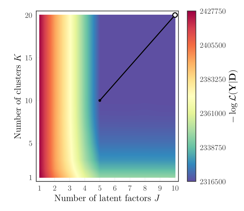
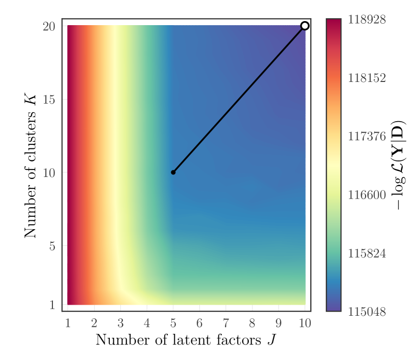
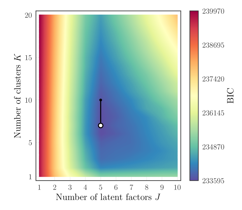
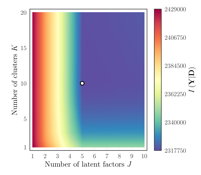
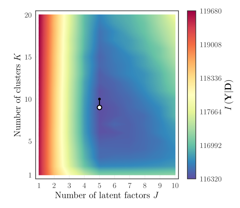
Figure 2: Metrics from our grid search for the toy model for two sample sizes: $N=100,000$ (left) and $N=5,000$ (right). The top panels show the negative log likelihood $-\log{\mathcal{L}\left(\textbf{Y}|\boldsymbol{\mathbf{\Psi}}\right)}$ evaluated at each combination of latent factors $J$ and number of clusters $K$ using the generated data in our toy model. The middle panels shows the BIC (Eq. 19) for those combinations, and the lower panel shows the message length. The white marker indicates the lowest value in each panel. A line connects to the true value (black point) to guide the eye.

We recorded the negative log likelihood, the BIC, and the message length for each permutation of $J$ and $K$. These metrics are shown in Figure 2. Unsurprisingly the negative log likelihood decreases with increasing numbers of latent factors $J$ and increasing numbers of components $K$. The lowest BIC value and message length is found at $J=5$ and $K=10$, identical to the true values.

It is clear from Figure 2 that a combination of latent factors and clustering in the latent space provides a better description of the (generated) data than a Gaussian mixture model without latent factors. Adding components to the model does improves the log likelihood, even with a single latent factor, but the addition of just one latent factor improves the log likelihood more so than adding twenty components. Not much more can be said for this example because the true data generating process is known, but this toy model does illustrate how clustering in high dimensional data can be better described by latent factors with clustering in the lower dimensional latent space.

Some technical background is warranted before we compare our estimated model parameters to the true values. We previously stated that the latent factors in this model are only identifiable up to an orthogonal rotation. That is to say that if the data were truly generated by latent factors $\textbf{L}_{\textrm{true}}$, then our estimates of those latent factors $\textbf{L}_{\textrm{est}}$ do not need to be identical to the true values. For example, the ordering of the estimated factors could be different from the true factors, and the ordering of the dimensionality in latent space would then be accordingly different. Since no constraint is placed on the ordering of the factor loads during expectation-maximization, there is no assurance (or requirement) that our factor loads match the true factor loads.

Another possibility is that the estimated factor loads could be flipped in sign relative to the true factor loads, and the scores would similarly be flipped. In both of these situations (reordering or flipped signs) the log likelihood given the data and the estimated factor loads $\textbf{L}_{\textrm{est}}$ would be identical to the log likelihood given the data and the true factor loads $\textbf{L}_{\textrm{true}}$ despite the difference in ordering and sign. The same can be said for any other scalar metric (e.g., Kullback-Leibler divergence; Kullback & Leibler, 1951). These examples serve to illustrate a more general property that the factor loads and factor scores can be orthogonally rotated by any valid rotation matrix $\boldsymbol{\mathbf{R}}$. The estimated factor loads $\textbf{L}_{\textrm{est}}$ could therefore appear very different from the true values, but they only differ by an orthogonal rotation. We discuss the impact of this limitation on real data in more detail in Section 4.

We took the model with the preferred number of latent factors and components found from a grid search ($K=10$, $J=5$; which are also the true values) and applied an orthogonal rotation to the latent space to be as close as possible to the true values. The rotation matrix $\mathbf{R}$ was found by solving for $J$ unknown angle parameters, each of which is used to construct a Givens rotation matrix (Givens, 1958), and then we take the product of those Givens matrices to produce a valid rotation matrix $\boldsymbol{\mathbf{R}}$. This process reduces to Euler angle rotation in three or fewer dimensions. This process rotates the latent space (L, $\boldsymbol{\mathbf{\xi}}$, $\boldsymbol{\mathbf{\Omega}}$), but has no effect on the model’s predictive power: the evaluated log likelihood or the Kullback-Leibler divergence (Kullback & Leibler, 1951) under the rotated model is indistinguishable from the unrotated model. In Figure 3 we show the estimated factor loads L, factor scores S, and specific variances $\boldsymbol{\mathbf{D}}$ compared to the true values. The agreement is excellent in all model parameters.

3.2 A toy model with data missing at random

Here we repeat the toy model used in the previous experiment, but we discard an increasing fraction of the data and evaluate the performance and accuracy of our method in the presence of incomplete data. We considered missing data fractions from 1% to 40%. In each case we treated the model parameters as unknown, assumed the missing data points were missing at random, and initialised the model as per Section 3.1.

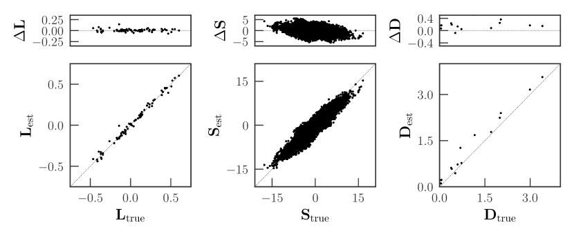
Figure 4: The estimated factor loads L (left), factor scores S (middle), and specific variances $\boldsymbol{\mathbf{D}}$ (right) compared to the true data generating values for Experiment 2 (Section 3.2). Here 40% of the data are missing at random. The agreement remains excellent, despite the large fraction of missing data entries. Note that the scales on the top panels are 2-10 times larger than those in Figure 3.

In Figure 4 we show the results of this experiment for our worst considered case, where 40% of the data entries are randomly discarded. We find that despite the high fraction of missing entries, our estimates of the model parameters remain unbiased in this example using a toy model. The corrections to our estimates of the specific variances are sufficient, in that the specific variance in each dimension is not systematically under-estimated from the true values, despite that 40% of the data entries are missing.

3.3 The Galah survey

In this experiment we perform blind chemical tagging using the photospheric abundances released as part of the second Galah data release (Buder et al., 2018). This data set includes up to 23 chemical abundances reported for 342,682 stars. In this example we chose to restrict ourselves to stars with a complete set of abundance measurements for a subset of those 23 elements (i.e., no missing data entries). For example, here we will exclude lithium and carbon abundances because the photospheric values will vary throughout a star’s lifetime (e.g., Casey et al., 2016b, 2019). This is true to a small degree for many elements (e.g., Dotter et al., 2017), but for the purposes of this experiment we assume that all other photospheric abundances remain constant throughout a star’s lifetime.

We first selected stars with flag_cannon = 0 to exclude stars where there is reason to suspect that the stellar parameters (e.g., $T_{\rm eff}$, $\log{g}$) are unreliable, and as a result the detailed chemical abundances would be untrustworthy. We then required all stars to have a signal-to-noise ratio exceeding 30 per pixel in the blue arm (snr_c1 > 30). We required that stars have no erroneous flags in all of the following abundances: Mg, Na, Al, Si, K, Ca, Sc, Ti, Mn, Fe, Ni, Cu, Zn, Y, Ba, La, and Eu. These elements were chosen because they trace multiple nucleosynthetic pathways, and they are more commonly reported in the Galah data release, allowing for a larger number of stars with a complete abundance inventory. There are 2,566 stars that met these criteria.

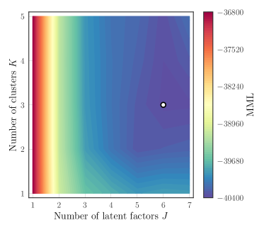
Figure 5: The top panel shows the negative log likelihood $-\log{\mathcal{L}\left(\textbf{Y}|\boldsymbol{\mathbf{\Psi}}\right)}$ evaluated at each combination of latent factors $J$ and number of clusters $K$ using Galah data in Experiment 3. The middle panel shows the BIC for those combinations, and the lower panel shows the message length. The white marker indicates the lowest value in each panel, showing the preferred number of latent factors and components.

We executed a grid search for the number of latent factors $J$ and the number of components $K$ that were preferred by the data. Starting with $J=1$ and $K=1$, we trialled each permutation of $J$ and $K$ up until $J=7$ and $K=5$. The results of this grid search are shown in Figure 5, where we show the negative log likelihood, the BIC, and message length found for each permutation. The behaviour of the BIC and the message length are very different here, unlike what was observed in our toy model. Here the BIC behaviour appears similar to the negative log likelihood in that the BIC prefers higher components and latent factors than the extent of the grid (e.g., $J>7$ and $K>5$). Indeed, if we were to trial higher values of $J$ and $K$ then the negative log likelihood would continue to increase. The model with six latent factors and three components ($J=6$, $K=3$) is found to have the shortest message length, which we take as our preferred model for these data.

Earlier we described how the latent factors we estimate can only be identified up until an orthogonal rotation. If we want to interpret the latent factors estimated from Galah data, then we must specify some target factor loads such that we can identify which factors are most similar to the yields we expect. We specified the following target latent factors where:

• The first factor load should have non-zero entries in Eu and La (e.g., the $r$-process).

• The second factor load should have non-zero entries in Ba, Y, and La (e.g., the $s$-process).

• The third factor load should have non-zero entries in Fe-peak elements Mn, Fe, Ni, Zn, and Ti.

• The fourth factor load should have non-zero entries in the odd-Z elements Na, Al, K.

• The fifth factor load should have non-zero entries in the $\alpha$-element tracers Si, Ca, and Mg.

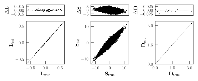
Figure 3: The estimated factor loads L (left), factor scores S (middle), and specific variances $\boldsymbol{\mathbf{D}}$ (right) compared to the true data generating values for Experiment 1 (Section 3.1). The agreement is excellent.

We initially set each non-zero entry in these target factor loads $\textbf{L}_{\textrm{target}}$ to $E^{-\frac{1}{2}}$, where $E$ is the number of non-zero entries in that factor load, to ensure that $\textbf{L}_{\textrm{target}}$ is mutually orthogonal. We solved for the $J$ unknown angles to produce a valid rotation matrix $\boldsymbol{\mathbf{R}}$ that would make our estimated loads L as close as possible to the target loads $\textbf{L}_{\textrm{target}}$, and then applied that rotation to the model. The target loads and (rotated) estimated loads are shown in Figure 6. Note that the purpose of this procedure is not to ‘find’ the target loads that we expect, but to provide as little information needed in order to identify and describe all factor loads within an astrophysical context. This procedure still requires that the factors be mutually orthogonal and that they describe the data. For these reasons, we will not always recover the exact target loads we seek: we will only be able to identify factor loads that are closest to the target loads.

This is demonstrated in Figure 6, where some estimated factor loads match closely to the target load (e.g., $\mathbf{L}_{2}$ which we identify as the s-process), and some barely match at all (e.g., $\mathbf{L}_{5}$). Here we show the absolute entry of the factor loads because even if an entry is negative, the corresponding factor scores could also be negative, and their product will contribute to the observed abundances. For this reason the sign does not matter here.

Some of these factor load entries may be non-zero because we require the latent factors to be mutually orthogonal, and not because they truly contribute to the data. To try and disentangle these possibilities, we calculate the fractional contribution that factor load makes to the observed abundances relative to other factor loads. We define the fractional contribution of the $j$th factor load to the $d$th data dimension as:

$$\mathbf{C}_{\textrm{d,j}}=\frac{\sum^{N}|\textbf{L}_{j,d}\textbf{S}_{n,j}|}{\sum^{J}\sum^{N}|\textbf{L}_{j,d}\textbf{S}_{n,j}|}\quad.$$ (36)

The fractional contributions to each element are shown in the right hand side of Figure 6. We identify the first factor $\mathbf{L}_{1}$ as being most similar to the r-process, and here it is the dominant contributor to Eu, a typical r-process tracer. Surprisingly we also find that this factor load is a reasonable contributor to the odd-Z element Sc. The specific scatter in Sc is 0.03 dex (Figure 7), suggesting that the Sc abundances are well-described by this latent factor model.

The second latent factor $\mathbf{L}_{2}$ here is most representative of the slow neutron capture process (s-process), with dominant contributions to Ba, and Y. This factor has some support at other elements, notably K. $\mathbf{L}_{3}$ is the primary contributor to nearly all Fe-peak elements, with close to negligible contributions from other factors. The exception here is Cu, where a near-equal contribution comes from $\mathbf{L}_{4}$. The fifth latent factor $\mathbf{L}_{5}$ is the dominant contributor to the $\alpha$-element tracers Si, Ca, and Mg, and surprisingly, Al. The specific scatter after accounting for these latent factors is smallest for Fe (0.01 dex) and largest for K (0.13 dex; Figure 7). The typical scatter in most elements is about 0.05 dex.

In Figure 8 we show the inferred clustering in latent space, where the separation between components is arguably best seen in the splitting between $\textbf{S}_{6}$ with respect to $\textbf{S}_{2}$ or $\textbf{S}_{3}$. When projected to data space (Figure 9) the third component (light green) is seen to have relatively higher abundance ratios of [K,Ba,Zn/Fe] at a given [Fe/H]. This is consistent with the clustering in latent space.

3.4 Galah survey data with an increasing number of stars with missing data entries

Here we extend our experiment in Section 3.3 to progressively include more stars, even though those stars have some abundance measurements missing. Specifically we started with the same subset of 2,566 stars in Section 3.3 and added a random set of stars that met our criteria of flag_cannon = 0 and snr_c1 > 30.

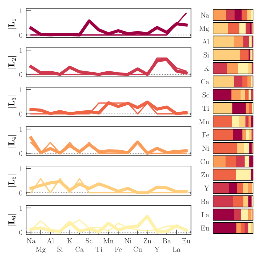
Figure 6: Latent factors inferred from 2,566 stars in Galah (Buder et al., 2018, thick lines) with 17 abundance measurements. Left panels show the absolute entries for each factor load, where the thin lines indicate the target latent factors (see Section 3.3). On the right we show the absolute fractional contributions to each element, ordered by the loads that contribute most.

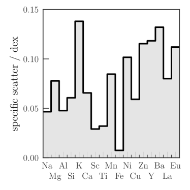
Figure 7: Specific scatter (e.g., $\sqrt{\boldsymbol{\mathbf{D}}}$) remaining in the Galah data (Buder et al., 2018) after accounting for the contributions by all latent factors.

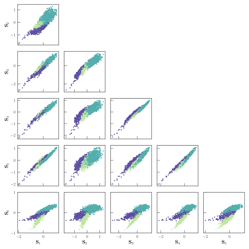
Figure 8: The factor scores S estimated in Experiment 3 (Section 3.3 using $N=$ 2,566 stars in the Galah data (Buder et al., 2018) that have 17 abundance measurements. Here each star is coloured by its inferred $K$th component.

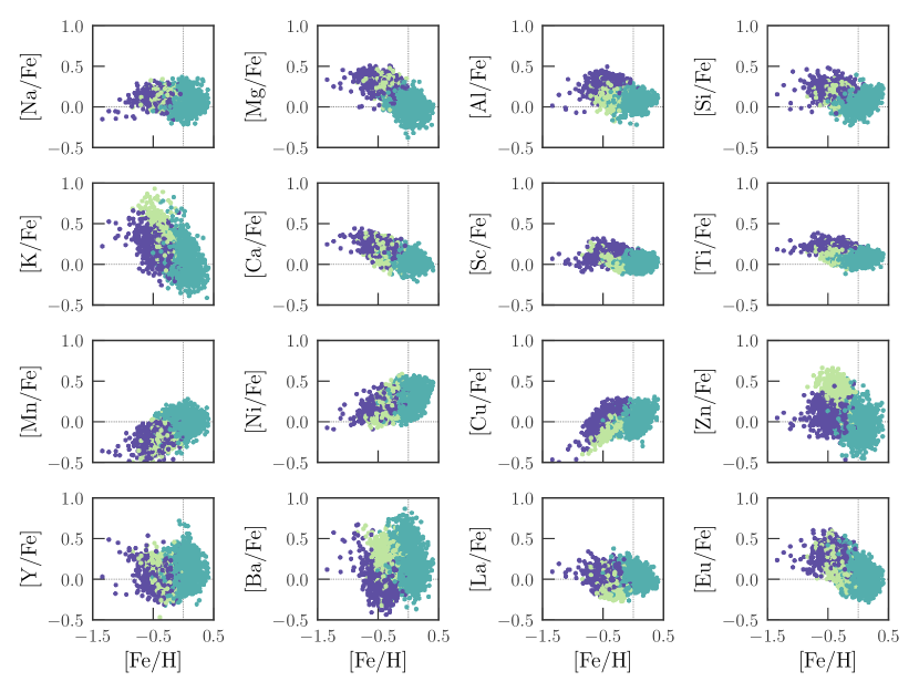
Figure 9: Detailed chemical abundances from the $N=$ 2,566 stars in Galah (Buder et al., 2018) that have 17 chemical abundances (Section 3.3). Each star is coloured by its $K$th inferred component from the lower-dimensional latent space, with the same colouring as per Figure 8.

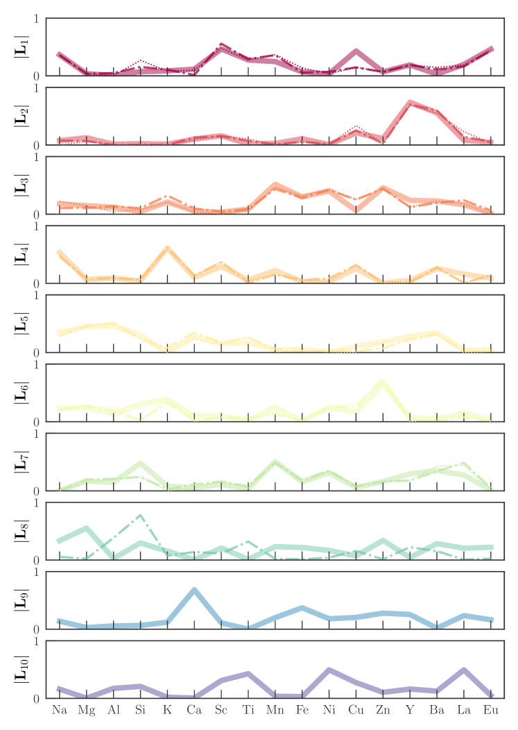
Figure 10: Latent factors found in Section 3.4 using different subsets of Galah data (Buder et al., 2018). The thin dotted line shows the result from Section 3.3 with $N=2,566$ stars with 17 abundances and no missing data. The thicker dot-dashed line indicates $N=12,566$ stars, of which $10,000$ have missing data entries. The thickest line has $N\sim 159,808$ stars, where ten latent factors are preferred.

4 Discussion

We have introduced a model to simultaneously account for the lower effective dimensionality of chemical abundance space, and perform clustering in that lower dimensional space. This provides a data-driven model of nucleosynthesis yields and chemical tagging that allows us to simultaneously estimate the latent factors that contribute to all stars, and cluster those stars by their relative contributions from each factor. The results are encouraging in that we find latent factors that are representative of the expected yields from dominant nucleosynthetic channels. However, the model that we describe is very likely not the correct model to use to represent chemical abundances of stars. Here we discuss the limitations of our model in detail.

We require latent factors to be mutually orthogonal in order to resolve an indeterminacy. This suggests an astrophysical context where the mean nucleosynthetic yields (integrated over all stellar masses and star formation histories) of various nucleosynthetic processes (e.g., $r$-process, $s$-process) are mutually orthogonal to each other. Clearly this assumption is likely to be incorrect: the nuclear physics of one environment where elements are produced will be very different from others, and there is no astrophysical constraint that those yields (or latent factors) should be mutually orthogonal. In principle one could represent the latent factors using a hierarchical data-driven model where the yields contribute as a function of stellar mass, metallicity, and other factors, but in principle to resolve the indeterminacy in this model would still require mutual orthogonality on the mean yields. Introducing a constraint on the factor scores that resolves this indeterminacy and allows for more flexible latent factors would be a worthy extension to this work.

The constraint of mutual orthogonality limits the inferences we want to make about stellar nucleosynthetic yields. For example, after accounting for all known sources of potassium production in the Milky Way, galactic chemical evolution models under-predict the level of K in the Milky Way by more than an order of magnitude (Kobayashi et al., 2006). From our inferences using Galah data, we find that $\textbf{L}_{2}$ – the factor we identify as the s-process – is the dominant contributor to potassium. This latent factor persists even in the presence of missing data, and a sample size two orders of magnitude larger. Does this suggest production of K is linked to the production of much heavier nuclei? If our model could confidently and reliably associate the production of K with other elements or sites then it could help explain the peculiar abundances of stars enhanced in K and depleted in Mg (Mucciarelli et al., 2012; Cohen & Kirby, 2012) – a chemical abundance pattern that currently lacks explanation (Iliadis et al., 2016; Kemp et al., 2018). In the Cohen & Kirby (2012) sample their high [K/Fe] stars also tend to be high in heavier elements, but there are also numerous abundance correlations present. However, is the K contribution that we infer physically realistic, or is it a consequence of requiring that the latent factors are mutually orthogonal? Distinguishing these possibilities is non-trivial, which is in part why caution is warranted when trying to interpret latent factor models. In this situation it is worth commenting that K has the largest specific scatter (Figure 7), suggesting that the contributions of K are perhaps not as well described by the latent factor model as other elements. This could in part be due to the non-trivial and significant effects that the assumption of local thermodynamic equilibrium (LTE) has on our inferred K abundances. These non-LTE effects are of order $0.5$ dex and will be accounted for in the upcoming Galah data release (S. Buder, private communication).

A similar argument could be made for Sc, where $\mathbf{L}_{1}$ – a factor load we identify as the r-process – is the primary contributor. Sc is under-produced in galactic chemical evolution models relative to observations (Kobayashi et al., 2006; Casey & Schlaufman, 2015). Based on this work, is the production of Sc linked to the production of heavy nuclei? Unlike K, the specific scatter in Sc is remarkably low: just 0.03 dex, among the best-described elements after Ti and Fe (0.01 dex). This would suggest that the latent factor model is a very good description for the production of Sc, but it does not prove that it is the description for the production of Sc.

There are other issues in our model that relate to our assumption of mutual orthogonality. Even if nucleosynthetic yields were truely mutually orthogonal, then the latent factors we infer are only identifiable up until an orthogonal basis. As we have seen in our experiments, the ordering and sign of the latent factors is not described a priori. This is both a feature and a bug: unrestricted ordering and signs allow for the model parameters to be estimated more efficiently because they can freely rotate as the model parameters are updated, but it does mean that we must ‘assign’ the latent factors we infer as being described by an astrophysical process (e.g., the first latent factor is r-process). A more general limitation of this is that the latent factors can be multiplied by some arbitrary rotation matrix, leading to latent factor loads that are very different from what was estimated by the model, but still lead to the exact same data (or log likelihood, or Kullback-Liebler divergence, etc). As a consequence, we can only ‘identify’ latent factors up until this rotation. We have sought to address this by constructing rotation matrices where the entries for each latent factor correspond to our expectations from astrophysical processes (whilst remaining orthogonal), but here we are limited by what astrophysical processes we are expecting to find within the constraint of being mutually orthogonal.

This in part constrains our ability to identify new nucleosynthetic processes. For example, let us consider a hypothetical situation where we would only expect there to be four nucleosynthetic processes that predominately contribute to the observed Galah abundances, but in practice we found that the data are best explained with five latent factors. We construct a rotation matrix where the first four latent factors describe the nucleosynthetic processes we expect to find. What of the fifth latent factor? We can constrain the possible values of the fifth latent factor conditioned on the requirement that all factors remain mutually orthogonal, but one can imagine that some (or perhaps many) elements have entries where the fifth latent factor can have near-zero or zero entries. Even if the mean nucleosynthetic yields are mutually orthogonal, there are scenarios that one can imagine where there is a limited amount we can say with confidence about that new nucleosynthetic process (see also Milosavljevic et al., 2018).

Notwithstanding these issues, we have shown that a latent factor model which allows for clustering in latent space can adequately describe chemical abundance data. We find six latent factors from a small subset of Galah data with complete abundances, and those latent factors can qualitatively be described within the context of astrophysical yields. Those latent factors are recovered in larger samples where the data are incomplete. That did not have to be the case: the mutually orthogonal latent factors could be entirely different from our expectations such that they did not have to match our expectations of nucleosynthetic yields. Indeed, the inferred factors – even after a valid rotation – could have made no astrophysical sense whatsoever. For this reason it is encouraging that there is some interpretability in the latent factors. Indeed, in the elements where we find surprising associations (e.g., Sc and K), these are elements where galactic chemical evolution models are most discrepant from observations, even after accounting for systematic errors in abundance measurements (e.g., violations to the assumption of local thermodynamic equilibrium).

In the subset of Galah data with complete abundances we find that three components are preferred. These components can be described as those with (1) low- and (2) high-[$\alpha$/Fe] abundance ratios, and another (3) primarily differing in K, Ba, and Zn abundances at a given [Fe/H] and [$\alpha$/Fe] abundance ratio. When we include $\sim$160,000 stars with up to 17 abundances, and assume the incomplete abundances are missing at random, we find that 16 components in latent space are preferred to explain the data. By construction these components are structured in their chemical abundances because of the projection from the latent space, and by extension of each component having similar chemistry, each component occupies realistic locations in a Hertzsprung-Russell diagram. When we project these component associations to the data space we find that none of the inferred components are structured or coherent in their positions or motions. However, in this sample of stars there are no gravitationally bound clusters where a reasonable (e.g. $\sim$30) number of stars have been observed. Clearly, more data would help to resolve a higher number of components.

Perhaps it is not so discouraging that none of the inferred components are structured in their positions or motions because there are no gravitationally bound clusters in the data. But there is clearly more that can be done in chemical tagging. Some components we infer have stars with positions and galactic orbits that would imply that they cannot have formed in the same star cluster. In these situations there is likely significant value in including joint probabilities on whether two stars could be associated to the same star formation site based on their dynamic properties. Similarly, although stellar ages are historically difficult to estimate precisely, can this imprecise information help inform weak priors or probabilities of two stars having the same association? There is an incredible amount of dynamical information available from Gaia, particularly for stars in the Galah survey, and weakly informative priors might be sufficient to help improve the granularity of chemical tagging without being overly constraining on the dynamical and star formation history we seek to infer.

5 Conclusions

We have introduced a data-driven model of nucleosynthesis by incorporating latent factors that are common to all stars, and allowing for clustering in the lower-dimensional latent space. This approach simultaneously allows us to efficiently tag stars based on their chemical abundances, and to infer the contributions that are common to all stars (e.g., nucleosynthetic yields). Experiments with generated data demonstrate that MML is a useful principle for selecting the appropriate number of latent factors and components. Experiments with Galah data reveal latent factors that are qualitatively and quantitatively similar to expected nucleosynthetic yields (e.g., products from the $s$-process, $r$-process, et cetera). Interestingly we find that deviations from expected yields occur in elements where observations and galactic chemical evolution models are most discrepant (e.g., K, Sc). While we advise caution in directly interpreting those latent factors as being nucleosynthetic yields, our model does provide the first data-driven approach to nucleosynthesis and chemical tagging. We advocate that more data, and the inclusion of weakly informative priors – joint probabilities using astrometry and a simplified model of the Milky Way – would help in realising the full potential of chemical tagging.

Documentation for the software that accompanies this paper is available at https://mcfa.rtfd.io. Below we provide code that generates ficticious data from a toy model and fits it.

⬇

import numpy as np

from mcfa import (mcfa, grid_search, mpl_utils, utils)

\parnp.random.seed(42)

\par# A boolean variable to indicate whether to perform a grid search

do_grid_search = (np.random.uniform() > 0.5)

\par# Generate data

X, true_theta = utils.generate_data(n_samples=1000,

n_features=15,

n_components=10,

n_latent_factors=5)

\par# The data, X, has shape (1000, 15)

assert X.shape == (1000, 15)

\parif do_grid_search:

# Perform a grid search for the number of components and latent factors.

J_trial = np.arange(1, 11) # trial from 1 to 10 latent factors

K_trial = np.arange(1, 21) # trial from 1 to 20 components

J_grid, K_grid, converged, metrics = grid_search.grid_search(J_trial, K_trial, X)

\par# Return the model with the smallest message length

model = metrics[”best_models”][”mml”]

\parelse:

# Or just fit the data given a number of components and latent factors.

model = mcfa.MCFA(n_components=10, n_latent_factors=5)

model.fit(X)

\par# Fitting quantities have a _ suffix

tau = model.tau_ # responsibility matrix

theta = dict(zip(model.parameter_names, model.theta_)) # model parameters

\par# Plot the factors.

fig_factors = mpl_utils.plot_factor_loads_and_contributions(model, X)

\par# Plot latent space.

fig_latent = mpl_utils.plot_latent_space(model, X)

\par# Plot data space, coloured by most probable component.

fig_data = mpl_utils.plot_data_space(model, X)

References

- Arthur & Vassilvitskii (2007) Arthur, D., & Vassilvitskii, S. 2007, in Proceedings of the eighteenth annual ACM-SIAM symposium on Discrete algorithms. (Society for Industrial and Applied Mathematics Philadelphia, PA, USA), 1027–1035
- Astropy Collaboration et al. (2013) Astropy Collaboration, Robitaille, T. P., Tollerud, E. J., et al. 2013, A&A, 558, A33
- Astropy Collaboration et al. (2018) Astropy Collaboration, Price-Whelan, A. M., Sipócz, B. M., et al. 2018, AJ, 156, 123
- Baek et al. (2010) Baek, J., McLachlan, G. J., & Flack, L. K. 2010, IEEE Transactions on Pattern Analysis and Machine Intelligence, 32, 1298
- Bland-Hawthorn et al. (2010a) Bland-Hawthorn, J., Karlsson, T., Sharma, S., Krumholz, M., & Silk, J. 2010a, ApJ, 721, 582
- Bland-Hawthorn et al. (2010b) Bland-Hawthorn, J., Krumholz, M. R., & Freeman, K. 2010b, ApJ, 713, 166
- Bland-Hawthorn & Sharma (2016) Bland-Hawthorn, J., & Sharma, S. 2016, Astronomische Nachrichten, 337, 894
- Bovy (2016) Bovy, J. 2016, ApJ, 817, 49
- Buder et al. (2018) Buder, S., Asplund, M., Duong, L., et al. 2018, The Monthly Notices of the Royal Astronomical Society, 478, 4513
- Casey et al. (2016a) Casey, A. R., Hogg, D. W., Ness, M., et al. 2016a, arXiv e-prints, arXiv:1603.03040
- Casey & Schlaufman (2015) Casey, A. R., & Schlaufman, K. C. 2015, ApJ, 809, 110
- Casey et al. (2016b) Casey, A. R., Ruchti, G., Masseron, T., et al. 2016b, MNRAS, 461, 3336
- Casey et al. (2017) Casey, A. R., Hawkins, K., Hogg, D. W., et al. 2017, ApJ, 840, 59
- Casey et al. (2019) Casey, A. R., Ho, A. Y. Q., Ness, M., et al. 2019, arXiv e-prints, arXiv:1902.04102
- Cohen & Kirby (2012) Cohen, J. G., & Kirby, E. N. 2012, ApJ, 760, 86
- Cramér (1946) Cramér, H. 1946, Mathematical Methods of Statistics (Princeton University Press)
- De Silva et al. (2015) De Silva, G. M., Freeman, K. C., Bland-Hawthorn, J., et al. 2015, MNRAS, 449, 2604
- Dempster et al. (1977) Dempster, A. P., Laird, N. M., & Rubin, D. B. 1977, Journal of the Royal Statistical Society: Series B (Statistical Methodology), 39, 1
- Dotter et al. (2017) Dotter, A., Conroy, C., Cargile, P., & Asplund, M. 2017, ApJ, 840, 99
- Dowe (2008) Dowe, D. L. 2008, Computer Journal, 51, 523 , Christopher Stewart WALLACE (1933-2004) memorial special issue
- Dowe (2011) Dowe, D. L. 2011, in Handbook of the Philosophy of Science - Volume 7: Philosophy of Statistics, ed. P. S. Bandyopadhyay and M. R. Forster (Elsevier), 901–982
- Dowe et al. (2007) Dowe, D. L., Gardner, S., & Oppy, G. 2007, The British Journal for the Philosophy of Science, 58, 709
- Dowe & Wallace (1997) Dowe, D. L., & Wallace, C. S. 1997, in Proc. Computing Science and Statistics - 28th Symposium on the interface, Vol. 28, 614–618
- Edwards & Dowe (1998) Edwards, R. T., & Dowe, D. L. 1998, in Lecture Notes in Artificial Intelligence (LNAI), Vol. 1394, Proceedings of the 2nd Pacific-Asia Conference on Research and Development in Knowledge Discovery and Data Mining (PAKDD-98), ed. X. Wu, R. Kotagiri, & K. B. Korb (Springer), 96–109
- Figueiredo & Jain (2002) Figueiredo, M. A. T., & Jain, A. K. 2002, IEEE Transactions on pattern analysis and machine intelligence, 24, 381
- Fitzgibbon et al. (2004) Fitzgibbon, L. J., Dowe, D. L., & Vahid, F. 2004, in Intelligent Sensing and Information Processing, 2004. Proceedings of International Conference on, IEEE, 439–444
- Freeman & Bland-Hawthorn (2002) Freeman, K., & Bland-Hawthorn, J. 2002, Annual Review of Astronomy and Astrophysics, 40, 487
- Givens (1958) Givens, W. 1958, in J. SIAM, 26–50
- Golub & Reinsch (1970) Golub, G. H., & Reinsch, C. 1970, Numerische mathematik, 14, 403
- Haar (1933) Haar, A. 1933, The Annals of Mathematics, 34, 147
- Ho et al. (2017a) Ho, A. Y. Q., Rix, H.-W., Ness, M. K., et al. 2017a, ApJ, 841, 40
- Ho et al. (2017b) Ho, A. Y. Q., Ness, M. K., Hogg, D. W., et al. 2017b, ApJ, 836, 5
- Hogg et al. (2016) Hogg, D. W., Casey, A. R., Ness, M., et al. 2016, ApJ, 833, 262
- Hotelling (1933) Hotelling, H. 1933, Journal of Educational Psychology, 24, 417
- Hunter (2007) Hunter, J. D. 2007, Computing in Science and Engineering, 9, 90
- Iliadis et al. (2016) Iliadis, C., Karakas, A. I., Prantzos, N., Lattanzio, J. C., & Doherty, C. L. 2016, ApJ, 818, 98
- Jones et al. (2001–) Jones, E., Oliphant, T., Peterson, P., et al. 2001–, SciPy: Open source scientific tools for Python, ,
- Kemp et al. (2018) Kemp, A. J., Casey, A. R., Miles, M. T., et al. 2018, MNRAS, 480, 1384
- Kluyver et al. (2016) Kluyver, T., Ragan-Kelley, B., Pérez, F., et al. 2016, in Positioning and Power in Academic Publishing: Players, Agents and Agendas, ed. F. Loizides & B. Schmidt, IOS Press, 87 – 90
- Knorr-Held (2000) Knorr-Held, L. 2000, Statistics in Medicine, 19, 1006
- Kobayashi et al. (2006) Kobayashi, C., Umeda, H., Nomoto, K., Tominaga, N., & Ohkubo, T. 2006, ApJ, 653, 1145
- Kullback & Leibler (1951) Kullback, S., & Leibler, R. A. 1951, The Annals of Mathematical Statistics, 22, 79
- Leung & Bovy (2018) Leung, H. W., & Bovy, J. 2018, MNRAS, 3062
- Martell et al. (2017) Martell, S. L., Sharma, S., Buder, S., et al. 2017, MNRAS, 465, 3203
- Milosavljevic et al. (2018) Milosavljevic, M., Aleo, P. D., Hinkel, N. R., & Vikalo, H. 2018, arXiv e-prints, arXiv:1809.02660
- Mitschang et al. (2014) Mitschang, A. W., De Silva, G., Zucker, D. B., et al. 2014, MNRAS, 438, 2753
- Mucciarelli et al. (2012) Mucciarelli, A., Bellazzini, M., Ibata, R., et al. 2012, MNRAS, 426, 2889
- Ness (2018) Ness, M. 2018, Publications of the Astronomical Society of Australia, 35, e003
- Ness et al. (2015) Ness, M., Hogg, D. W., Rix, H. W., Ho, A. Y. Q., & Zasowski, G. 2015, ApJ, 808, 16
- Ness et al. (2018a) Ness, M., Rix, H. W., Hogg, D. W., et al. 2018a, ApJ, 853, 198
- Ness et al. (2018b) —. 2018b, ApJ, 853, 198
- Oliver et al. (1996) Oliver, J. J., Baxter, R. A., & Wallace, C. S. 1996, in ICML, 364–372
- Pérez & Granger (2007) Pérez, F., & Granger, B. E. 2007, Computing in Science and Engineering, 9, 21
- Portegies Zwart et al. (1998) Portegies Zwart, S. F., Hut, P., Makino, J., & McMillan, S. L. W. 1998, A&A, 337, 363
- Price-Jones & Bovy (2018) Price-Jones, N., & Bovy, J. 2018, MNRAS, 475, 1410
- Rao (1945) Rao, C. R. 1945, in Bulletin of the Calcutta Mathematical Society., 81–89
- Schwarz (1978) Schwarz, G. 1978, The Annals of Statistics, 6, 461
- Shannon (1948) Shannon, C. E. 1948, Bell System Technical Journal, 27, 379
- Sheinis et al. (2015) Sheinis, A., Anguiano, B., Asplund, M., et al. 2015, Journal of Astronomical Telescopes, Instruments, and Systems, 1, 035002
- Stewart (1980) Stewart, G. W. 1980, SIAM Journal on Numerical Analysis, 17, 403
- Taylor (2005) Taylor, M. B. 2005, in Astronomical Society of the Pacific Conference Series, Vol. 347, Astronomical Data Analysis Software and Systems XIV, ed. P. Shopbell, M. Britton, & R. Ebert, 29
- Thompson (2004) Thompson, B. 2004, Exploratory and confirmatory factor analysis: Understanding concepts and applications. (American Psychological Association), doi:10.1037/10694-000
- Ting et al. (2019) Ting, Y.-S., Conroy, C., Rix, H.-W., & Cargile, P. 2019, ApJ, 879, 69
- Ting et al. (2012) Ting, Y. S., Freeman, K. C., Kobayashi, C., De Silva, G. M., & Bland-Hawthorn, J. 2012, Monthly Notices of the Royal Astronomical Society, 421, 1231
- Tipping & Bishop (1999) Tipping, M. E., & Bishop, C. M. 1999, Journal of the Royal Statistical Society: Series B (Statistical Methodology), 61, 611
- Viswanathan et al. (1999) Viswanathan, M., Wallace, C., Dowe, D. L., & Korb, K. 1999, Advanced Topics in Artificial Intelligence, 405
- Wallace (1995) Wallace, C. S. 1995, Technical report, Department of Computer Science, Monash University, 95, 21
- Wallace (2005) Wallace, C. S. 2005, Statistical and inductive inference by minimum message length (Springer Science & Business Media)
- Wallace & Dowe (1994) Wallace, C. S., & Dowe, D. L. 1994, in Proc. 7th Australian Joint Conf. on Artificial Intelligence (World Scientific), 37–44
- Wallace & Dowe (1999) Wallace, C. S., & Dowe, D. L. 1999, Computer Journal, 42, 270
- Wallace & Dowe (2000) —. 2000, Statistics and Computing, 10, 73
- Wallace & Freeman (1987) Wallace, C. S., & Freeman, P. R. 1987, Journal of the Royal Statistical Society: Series B (Statistical Methodology), 49, 240
- Walt et al. (2011) Walt, S. v. d., Colbert, S. C., & Varoquaux, G. 2011, Computing in Science and Engg., 13, 22
- West & Heger (2013) West, C., & Heger, A. 2013, ApJ, 774, 75